A Characterization of the ALMA Phasing System at 345 GHz

Abstract

The development of the Atacama Large Millimeter/submillimeter Array (ALMA) phasing system (APS) has allowed ALMA to function as an extraordinarily sensitive station for very long baseline interferometry (VLBI) at frequencies of up to 230 GHz ($\lambda\approx$1.3 mm). Efforts are now underway to extend use of the APS to 345 GHz ($\lambda\approx$0.87 mm). Here we report a characterization of APS performance at 345 GHz based on a series of tests carried out between 2015–2021, including a successful global VLBI test campaign conducted in 2018 October in collaboration with the Event Horizon Telescope (EHT).

1 Introduction

In addition to operating as a connected element interferometer, the Atacama Large Millimeter/submillimeter Array (ALMA) can function as the equivalent of a single very large aperture antenna if the data from its individual antennas are phase-corrected and coherently added. The development of a phased-array capability for ALMA (Doeleman et al., 2009; Matthews et al., 2018) has allowed ALMA to play a transformational role in the technique of very long baseline interferometry (VLBI) at millimeter (mm) wavelengths. By boosting the sensitivity of VLBI baselines in previously existing arrays operating at 230 GHz ($\lambda\approx$1.3 mm) by up to an order of magnitude, phased ALMA was crucial to the achievement of the first horizon scale images of the supermassive black hole at the center of the M87 Galaxy, M87* (Event Horizon Telescope Collaboration et al., 2019a, b, c, d, e, f) and the one at the center of our own Milky Way, Sgr A* (Event Horizon Telescope Collaboration et al., 2022a, b, c, d, e, f). At 86 GHz ($\lambda\approx$3 mm), phased ALMA was also key to achieving the first scatter-corrected images of SgrA*, the supermassive black hole candidate at the Galactic Center (Issaoun et al., 2019) and the first ALMA detection of pulsed emission from radio pulsars (Liu et al., 2019, 2021).

The ALMA phasing system (APS) has been offered to the community for VLBI science observations in ALMA Bands 3 ($\lambda\approx$3 mm; $\nu\approx 86$ GHz) and 6 ($\lambda\approx$1.3 mm; $\nu\approx 230$ GHz), where the Global mm-VLBI Array (GMVA) and the Event Horizon Telescope (EHT), respectively, serve as partner networks. The first science observations that included the APS in this capacity were conducted in 2017 April as part of ALMA Cycle 4 (Goddi et al., 2019). To further expand scientific possibilities, there is now growing motivation to push VLBI techniques to still shorter wavelengths, i.e., $\lambda\approx$0.87 mm or $\nu\approx$345 GHz (e.g., Falcke et al., 2001; Miyoshi & Kameno, 2002; Weintroub, 2008; Krichbaum et al., 2008; Doeleman et al., 2009; Event Horizon Telescope Collaboration et al., 2019a, b). Not only will this enable even higher angular resolution ($\lesssim 20\mu$as for Earth-sized baselines), but it will help to improve $uv$ coverage by enabling the combination of 230 GHz and 345 GHz observations (thus enabling higher fidelity imaging), and will minimize the effects of interstellar scattering on achievable image quality. The latter is particularly important for imaging SgrA*, where interstellar ionized gas along the line-of-sight causes significant blurring of images at longer radio wavelengths (Johnson & Gwinn, 2015; Johnson, 2016; Event Horizon Telescope Collaboration et al., 2022g).

A key component of the effort to extend VLBI capabilities into the sub-mm regime is the extension of ALMA’s phased array capabilities to 345 GHz. While this had been an envisioned application of the APS since its conception (e.g., Doeleman, 2010; Fish et al., 2013), commissioning of ALMA’s phasing capabilities was initially limited to the 86 GHz and 230 GHz bands (ALMA Band 3 and 6, respectively) owing to time constraints and to the limited availability of suitably equipped VLBI partner sites (see Matthews et al., 2018).

While the APS itself is agnostic to observing frequency, there are practical considerations that impact the use of the APS at $\nu~{}\hbox to0.0pt{$>$\hss}{\lower 4.30554pt\hbox{$\sim$}}$345 GHz and the optimization of phasing efficiency at higher frequencies. One of the most important is the shorter coherence timescales at higher frequencies owing to the effects of tropospheric water vapor, which become increasingly significant with increasing baseline length. This in turn will impact choices such as the maximum baseline length to include in the phased array and whether or not to apply “fast” phasing corrections—derived from water vapor radiometer (WVR) data at each ALMA antenna—in addition to the nominal “slow” phasing corrections derived by the phasing engine within the (TelCal) telescope calibration software (Matthews et al., 2018). Additionally, effects such as pointing errors and wind speeds will have increasingly important impacts on phased array performance at higher frequency owing to the smaller beam size of the antennas (see, e.g., Smith et al., 2000).

Here we present a characterization of the performance and phasing efficiency of the APS at 345 GHz based on test sessions conducted between 2015 March and 2021 September. The data sets include observations obtained in 2018 as part of a multi-day global VLBI test campaign that produced for the first time VLBI fringes in the 345 GHz band (Event Horizon Telescope Collaboration et al., in preparation; hereafter Paper II).

2 Observations

Testing and characterization of the performance of the APS for use in Band 7 were done using a combination of ALMA standalone tests and a global VLBI campaign. These tests are described in detail in the next two subsections. In the discussions of phased ALMA that follow, we adopt the following nomenclature: the reference antenna is a designated antenna relative to which the phasing corrections are computed for all other antennas; the sum antenna is a virtual antenna containing the phased signals of all of the phased-array antennas summed together; a comparison antenna is an ALMA antenna that is participating in the observations, but is not being phased and is not included in the phased sum.

2.1 Initial Testing: ALMA Standalone Observations

Initial testing of the APS at 345 GHz began in 2015 and continued throughout 2021 with a series of short ALMA standalone tests. These observations were conducted during ALMA Extension and Optimization of Capabilities (EOC) time or Engineering time, and typically lasted from a few minutes up to 40 minutes. A summary of these tests is provided in Table 1, including array and weather parameters.

Selected observing targets comprised bright ( $>$$\sim$1 Jy at 345 GHz) quasars and other compact extragalactic sources that are unresolved on intra-ALMA baselines. Most of the target quasars are routinely observed at ALMA as part of the flux-density monitoring program with the ALMA Compact Array (ACA). This program includes measurements, mostly in Band 3 and Band 7, of bright reference sources, referred to as ”Grid Sources” (Remijan et al., 2019)).

Data from these standalone APS tests allowed us to demonstrate the feasibility of phased ALMA operations at sub-mm wavelengths. Although in several instances the test data were taken in conditions that were sub-optimal for Band 7 observing, such data enable exploration of the impacts of weather conditions on phasing performance and help to establish guidelines on the parameter space for scientifically useful phasing operations at higher frequencies (e.g. maximum baseline length in the phased array, maximum wind speed). More details on the analysis of these test datasets are given in Section 3.

2.2 The 2018 Global VLBI Test Campaign

2018 October marked the first time that ALMA’s 345 GHz phasing capability was tested over a sustained observing session, as well as during a global VLBI campaign, with the goal of obtaining 345 GHz VLBI fringes on global baselines (see Paper II). During this campaign, APS operations at 345 GHz were characterized during a series of four observing windows from October 17–21. A total of six ALMA scheduling blocks were built and executed, including four blocks in Band 7 (each spanning $\sim$90 min) and two blocks in Band 6 (each spanning $\sim$35 min) for comparison purposes. A summary of the observations is reported in Table 2.

Table 1: Standalone ALMA Band 7 Phasing Tests

UTC Starta	UTC Enda	Archive UIDb	$N_{\rm phased}$	Baselinesc	PWVd	Wind Speedd	$\eta_{v}$e	Qual.f
(YYYY MMM DD/hh:mm:ss.s)	(YYYY MMM DD/hh:mm:ss.s)			(m)	(mm)	(m s-1)
2015 Mar 30/02:49:26.4	2015 Mar 30/02:51:46.9	uid___A002_X9cdda2_X42c	9	15–193	0.53$\pm$0.03	8.5$\pm$2.5	0.86	0.91
2015 Aug 02/14:37:58.7	2015 Aug 02/14:45:01.4	uid___A002_Xa73e10_X28dc	35	15–1492	0.50$\pm$0.04	7.5$\pm$4.5	0.46	0.94
2016 Jul 10/08:51:25.1	2016 Jul 10/09:38:54.0	uid___A002_Xb53e10_Xa7a	9	19-396	2.0$\pm$0.5	7$\pm$5	0.15	0.66
2017 Jan 30/21:47:33.5	2017 Jan 30/21:51:58.4	uid___A002_Xbd3836_X4ba	37	15–260	5.0$\pm$1.5	12$\pm$5	0.07	0.36
2017 Jan 30/21:56:56.8	2017 Jan 30/22:08:59.2	uid___A002_Xbd3836_X579	37	15–260	5.0$\pm$1.5	13$\pm$6	0.10	0.50
2017 Jan 30/22:18:57.0	2017 Jan 30/22:34:29.2	uid___A002_Xbd3836_X739	37	15–260	4.5$\pm$1.2	14$\pm$6	0.16	0.66
2017 Jan 30/22:39:27.4	2017 Jan 30/22:51:29.2	uid___A002_Xbd3836_X87c	37	15–260	4.5$\pm$1.5	13$\pm$4	0.11	0.55
2017 Feb 01/03:19:27.0	2017 Feb 01/04:02:59.7	uid___A002_Xbd3836_X4363g	41	15–331	1.6$\pm$0.6	9$\pm$5	0.75	0.93
2019 Mar 08/04:12:43.8	2019 Mar 08/04:19:14.4	uid___A002_Xd9435e_X2859	45	15–314	1.0$\pm$0.1	3.5$\pm$3.5	0.74	0.95
2021 Mar 23/23:13:24.1	2021 Mar 23/23:21:11.3	uid___A002_Xea64a8_X321	33	15–1232	2.7$\pm$0.15	10$\pm$4	0.49	0.88
2021 Mar 24/21:37:20.6	2021 Mar 24/21:44:11.3	uid___A002_Xea6cf9_X1c1	33	15–1214	2.15$\pm$0.25	12$\pm$5	0.21	0.84
2021 Mar 25/01:07:24.7	2021 Mar 25/01:15:11.3	uid___A002_Xea6cf9_Xb5a	35	15–1231	2.55$\pm$0.15	4$\pm$3	0.38	0.90
2021 Mar 25/19:12:42.6	2021 Mar 25/19:20:11.3	uid___A002_Xea6cf9_X1d9e	25	22–969	2.0$\pm$0.2	13$\pm$5	0.11	0.69
2021 Aug 26/19:55:06.2	2021 Aug 26/20:02:18.0	uid___A002_Xefb0d3_X7c2	31	92–6855	1.2$\pm$0.2	12$\pm$8	0.21	0.72
2021 Sep 02/19:37:24.1	2021 Sep 02/19:45:11.6	uid___A002_Xf02179_X1ea	25	237–6855	0.45$\pm$0.15	10$\pm$6	0.26	0.87
2021 Sep 03/02:07:24.7	2021 Sep 03/02:15:29.9	uid___A002_Xf02179_X10a0	29	237–6855	0.4$\pm$0.1	4$\pm$3	0.65	0.91

Table 2: Observations Log for 2018 October Band 7 Test Campaign

UTC Start	UTC End	Archive UID	$N_{\rm phased}$	PWV	Wind Speed	$\eta_{v}$	Qual.	Band
(YYYY MMM DD/hh:mm:ss.s)	(YYYY MMM DD/hh:mm:ss.s)			(mm)	(m s-1)
2018 Oct 16/23:42:52.4	2018 Oct 17/01:00:26.0	uid___A002_Xd3607d_X6f14	23	$2.0\pm 0.3$	$9\pm 5$	0.13	0.42	7
2018 Oct 17/01:05:24.6	2018 Oct 17/01:40:54.3	uid___A002_Xd3607d_X70fe	23	$2.5\pm 0.5$	$7\pm 3$	0.10	0.37	6
2018 Oct 17/09:31:07.1	2018 Oct 17/11:02:16.5	uid___A002_Xd36f86_X24dd	25	$1.8\pm 0.8$	$12\pm 4$	0.07	0.28	7
2018 Oct 18/23:23:08.3	2018 Oct 19/00:52:37.4	uid___A002_Xd37ad3_X7ef1	25	$1.1\pm 0.3$	$6\pm 4$	0.37	0.91	7
2018 Oct 19/00:58:00.0	2018 Oct 19/01:32:54.5	uid___A002_Xd37ad3_X82a2	25	$1.0\pm 0.1$	$4\pm 3$	0.51	0.96	6
2018 Oct 21/09:12:54.4	2018 Oct 21/10:59:18.3	uid___A002_Xd395f6_Xd41f	29	$0.85\pm 0.10$	$3\pm 3$	0.93	0.97	7

Table 3: VLBI Sources Observed During the 2018 October Band 7 Test Campaign

Source	UTC Starta	UTC Enda	Band	Calibration Intentb
	(YYYY MMM DD/hh:mm:ss)	(YYYY MMM DD/hh:mm:ss.s)
CTA102	2018 Oct 18/23:43:25	2018 Oct 18/23:58:05	7	…
3C454.3	2018 Oct 19/00:06:25	2018 Oct 19/00:20:15	7	Flux
BL Lac	2018 Oct 19/00:29:25	2018 Oct 19/00:43:15	7	…
BL Lac	2018 Oct 19/01:02:25	2018 Oct 19/01:23:58	6	…
J0423–0120	2018 Oct 21/09:21:25	2018 Oct 21/09:43:15	7	Bandpass
J0510+1800	2018 Oct 21/09:52:25	2018 Oct 21/10:06:15	7	Polarization
J0510+1800	2018 Oct 21/10:16:25	2018 Oct 21/10:28:41	7	Polarization
J0522–3627	2018 Oct 21/10:36:25	2018 Oct 21/10:59:18	7	…

Table 4: ALMA Frequency Settings

Band	Central Freq. (GHz)				Chan. Width	No. Spec.	Integ. time
($\lambda$)	SPW 0	SPW 1	SPW 2	SPW 3	(MHz)	Chans.	(s)
6 (1.3 mm)	213.1	215.1	227.1	229.1	7.8125	240a	4.03
7 (0.85 mm)	335.5	337.5	347.7	349.7	15.625	120	4.03

Table 5: ALMA Source Flux Densities from the 2018 October Band 7 Test Campaign

Source	$S_{0}$ (Jy)	$S_{1}$ (Jy)	$S_{2}$ (Jy)	$S_{3}$ (Jy)	$\overline{S}$ (Jy)	$S_{\rm arch}$ (Jy)	Ratio	$\Delta t_{S}$ (days)
Flux Calibrator = 3C454.3, S343GHz = 3.53 Jy, $\alpha$=$-$0.69
(1)	(2)	(3)	(4)	(5)	(6)	(7)	(8)	(9)
CTA102	1.42	1.41	1.40	1.40	1.41	1.68	0.84	0
BL Lac (Band 7)	1.06	1.06	1.05	1.05	1.06	1.11	0.95	+71
BL Lac (Band 6)	1.26	1.25	1.22	1.24	1.24	…	…	…
J0423-0120	2.48	2.50	2.44	2.43	2.46	2.24	1.1	0
J0510+1800	1.23	1.24	1.22	1.21	1.22	1.28	0.95	0
J0522$-$3627	4.91	4.94	4.87	4.84	4.89	4.32	1.13	0

2.2.1 Observed Targets

As for the standalone phasing tests in Table 1, selected observing targets comprised bright quasars and other compact extragalactic sources. An effort was made to select sources that would be point-like on the angular scales sampled by intra-ALMA baselines (to maximize phasing efficiency), while still having sufficient correlated flux density to allow high signal-to-noise ratio (SNR) fringe detections with short integration times on VLBI baselines. This is particularly important in Band 7, where coherence timescales are expected to be only $\sim$10 s (e.g., Doeleman et al., 2011).

A list of observed sources and their calibration intent is given in Table 3; only VLBI targets observed on October 18/19 and 21 are listed (targets observed on previous days were not included in the analysis owing to poor weather conditions; see Sect. 2.2.3 and Appendix A). In most cases, recent flux density measurements at 230 and 345 GHz were available from the ALMA Calibrator Source Catalogue. These can be used for cross-comparison and validation of the APS performance and calibration in Band 7 (see Section 5.1).

2.2.2 Observational Setup

During the 2018 October test campaign the ALMA antennas were in transition from configuration C43-6 (maximum baseline 2500 m) to C43-5 (maximum baseline 1400 m). There were 23–29 12 m antennas included in the ALMA phased array (depending on the session), with a phasing radius limited to 300 m. An additional 16–22 outlying antennas (with maximum baselines between 1400 m and 2500 m, depending on the day) were withheld for comparison purposes. Antenna locations are plotted in Figure 1. The observing array was more extended than during previous science observations in VLBI mode, where only antennas within a radius of 180 m were phased (e.g., Goddi et al., 2019). Only 12 m antennas were included in the array; ALMA’s 7 m CM antennas can also be used with the APS, but are typically excluded from phased-array operations for a variety of practical reasons.

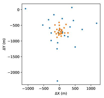
Figure 1: ALMA antenna locations for the phased array (orange points) and the unphased comparison antennas (blue points) during the Band 7 phasing tests in 2018 October. Positions are plotted with positive values of $X$ toward local east and positive values of $Y$ toward local north.

The spectral setup included four spectral windows (SPWs), each with a bandwidth of 1875 MHz, that were processed by the ALMA Baseline Correlator. Two SPWs were in the lower sideband and two in the upper sideband. In Band 7 the data outputted by the ALMA Baseline Correlator were averaged in frequency to produce 120 channels per SPW (corresponding to a channel spacing of 15.625 MHz). In Band 6 there were 240 channels per SPW (resulting in a channel spacing of 7.8125 MHz). The frequency setup is summarized in Table 4. The spectral data from the ALMA Baseline Correlator are available with a time resolution of 4.032 s. In parallel, VLBI recordings of all four basebands, each corresponding to one of the four SPWs, were recorded in dual linear polarizations, thus exercising the full 64 Gb s^-1 VLBI recording capability at ALMA (see Paper II).

2.2.3 Weather Conditions

During the 2018 October campaign there were no significant technical issues at ALMA and all aspects of its phasing and VLBI systems appeared to be performing nominally. However, with the exception of the last observing night where conditions were exceptional, weather conditions did not meet the usual requirements for Band 7 observing at ALMA. As discussed below, these weather issues significantly impacted the quality of the phased array data, but at the same time provided valuable insights into the range of weather conditions where scientifically useful phased array operations in Band 7 are likely to be possible.

In the first two sessions of the campaign there was high and variable precipitable water vapor (PWV$\gtrsim$2 mm) and high wind speeds ($\gtrsim$10–15 m s^-1; see Table 2 and Figure 10 in Appendix C). These factors led to unstable atmosphere conditions over timescales of a few seconds, which compared unfavorably with the $\sim$ 18 second loop time of the “slow” APS phasing solutions (see Matthews et al., 2018; Goddi et al., 2019). The phasing efficiency, $\eta_{v}$ (see Appendix C and Eq. C2), was consequently rather low: typical values reported by TelCal during the observations ranged from 5%–20%, and for portions of the session ALMA appeared to be effectively unphased (see Section 4).

At the onset of the third session (on the night of October 18/19), atmospheric stability was significantly improved compared with the previous two VLBI sessions. Finally, during the fourth and final VLBI session (corresponding to the fifth day of the VLBI observing window), weather at ALMA was excellent, with precipitable water vapor (PWV) $\sim$0.8 mm and wind speeds of only a few m s^-1 (see Table 2 and the bottom panel of Figure 10 in Appendix C). Throughout the latter session, the estimated phasing efficiency reported by TelCal was consistently $>$90%, and frequently above 95% (see Section 4).

3 APS Performance Metrics

One effective way to visualize the APS performance is through plots of the phasing efficiency, $\eta_{v}$ (see Eq. 3 in Appendix E). For monitoring purposes, this quantity is computed by TelCal for a designated comparison antenna and can be extracted from the archival science data model (ASDM) file metadata (see also Goddi et al., 2019). Some details about how and why this is done are discussed in Appendix E.

An additional figure-of-merit computed by TelCal is a ‘quality’ metric, which is a figure of merit intended to provide a sense of the goodness-of-fit of the phasing calculations. It is constructed from the RMS of the phase residuals, $\sigma_{\rm RMS}$, and assumes values ranging between 0 (no solution) to 1 (excellent fit). Noting that in the case of pure noise this value is $\sigma_{\rm RMS,max}~{}=~{}\pi/\sqrt{3}$ (Thompson et al., 2017), a quality metric for each fit may be constructed as $q~{}=~{}(\sigma_{\rm RMS,max}-\sigma_{\rm RMS})/\sigma_{\rm RMS,max}$.

Both are plotted in Figure 2 for the 2018 October data, arranged by correlator subscan (i.e. the interval of the phasing solution), with the data for each time interval averaged over all basebands. This plot shows that in the 2018 October test, the APS has achieved 90% phasing efficiency on October 21, which was the goal specified in the original operational requirements (Matthews et al., 2018). On October 18/19 the phasing efficiency was rather modest, which is ascribable to poor atmospheric conditions (see Section 4), but still of good quality. This situation occurs in cases where the phase-solving algorithm is able to find good-quality solutions, but atmospheric conditions are varying sufficiently rapidly that the 16-second time delay in the application of these “slow” phasing corrections to the data renders them “stale” and no longer optimal. The contrast between these days and the first two makes clear that the quality metric is a useful discriminator between different causes of low-phasing efficiency. During the first two observing sessions where wind speeds were high (October 16/17 and October 17) $\eta_{v}$ is low and the quality metric is $<<1$. On the other hand, for October 18/19, the quality metric is consistently $\sim$1 despite periods of low $\eta_{v}$, suggesting that rapid variations in water vapor rather than wind effects were the dominant source of efficiency loss.

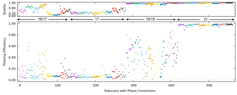
Figure 2: Phasing efficiency ($\eta_{v}$, as defined in Eq. E2; lower panel) and quality (top panel) during the phased-array test in Band 7 as part of the 2018 October VLBI campaign. Calendar dates and their respective time ranges are indicated by the arrows between the two panels. All scans are plotted and colored by science target for each day. The phasing “quality” is a “goodness-of-fit” parameter derived from the fitting process, which is scaled so that unity corresponds to perfect phasing. The phasing efficiency ranges from 0 (totally un-phased) to 1 (perfect phasing). The large departures of efficiency below 0.8 (on days from 16 to 19) correspond to poor atmospheric conditions (see Section 4).

An alternative way to display the APS performance during observations is to plot directly amplitudes and phases of the interferometric visibilities including the sum and the reference antennas, on baselines to one or more comparison antennas. In Figure 3 (left panels) we show a comparison of the correlated amplitude as a function of time for the 2018 October data on: (i) baselines between the phasing reference antenna and each of two different unphased comparison antennas; and (ii) baselines between the phased sum antenna and the same comparison antennas. For an optimally phased array, the correlated amplitude of (ii) should ideally improve by a factor of $\sim\sqrt{N_{\rm phased}}$ when phasing is active. Plots of (i) are useful in making this assessment. We see that for October 16/17 and October 17, the correlated amplitude for a baseline with the phased sum is comparable to that on a baseline with a single antenna, implying that the array is effectively unphased as a result of the poor weather conditions. On October 19, the phased sum shows a significant improvement in correlated amplitude (green points), though the data are noisy and the improvement does not match the ideal $\sqrt{N_{\rm phased}}$ scaling. Finally on October 21 nearly ideal phasing performance is seen.

In Figure 3 (right panels) we show phase versus time on baselines which are part of the phased sum for the same four data sets. On October 21 the phases in individual scans show a low RMS dispersion and are tightly clustered near 0, except for a few seconds near the start-up of each scan, when the phases are still being adjusted. (Note that the scan at 10:06 UT was passively rather than actively phased, hence the higher noise level). On October 19 some hints of phase coherence are seen, but the data are much noisier. Finally on October 16/17 and 17 the phases appear nearly random, consistent with an unphased array.

The performance of the APS in Band 7 relative to Band 6 is discussed in Section 4.3. Although the weather conditions were sub-optimal during the test observations, we nonetheless see comparable RMS phase fluctuations in the two bands, suggesting that there is no systematic degradation in phasing performance in Band 7 compared to Band 6.

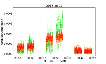
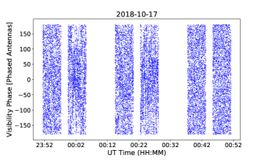
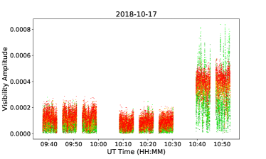
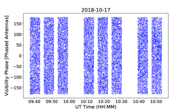
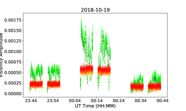
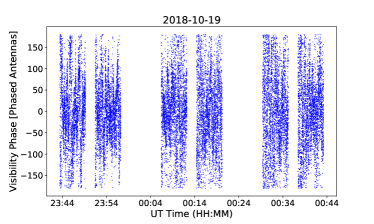
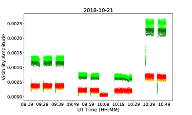
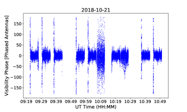
Figure 3: Illustration of the performance of the APS during the 345 GHz (Band 7) VLBI experiment on 2018 October 16/17, 17, 18/19, 21 (from top to bottom). Left panels: correlated amplitude is plotted as a function of time on two sets of baselines: (1) the phasing reference antenna with two unphased comparison antennas (red points); (2) the phased sum antenna with the same comparison antennas (green points). Right panels: phase versus time is plotted on baselines between the ALMA reference antenna and the other phased ALMA antennas (blue points). The uncorrelated phases during the first few integrations of each observing block (lower-right panel), are due to the fact that phases are still being adjusted (i.e. the array is unphased; see §3). In both columns, data from a single correlator quadrant (baseband 3, corresponding to SPW = 2 in Table 4) and a single polarization (XX) are shown. Data in the other SPWs and polarization YY show similar behaviors.

4 Variables Impacting Phased Array Performance in Band 7

Because the data recorded during the Band 7 APS tests presented in Section 2 were acquired using different arrays of ALMA antennas and across a range of weather conditions, this allows us to begin to investigate how different array parameters, weather conditions, and other variables affect APS performance in Band 7. These effects are discussed in the following subsections.

4.1 Impact of Weather Conditions

The four dates of the 2018 October campaign were conducted with a phased array with a fixed radius (300-m) and all included a similar number of phased antennas ($\sim$25). However, weather conditions varied on the different days. We can therefore use the 2018 data to assess how weather conditions affect the APS performance.

In Section 2.2.3 we point out that observations on October 16 and 17 were plagued by variable PWV and high winds (see also Appendix C). Under these conditions, it was not possible to successfully phase the array, with the phased sum antenna performing no better than a single antenna. Under conditions of moderate wind but still relatively high PWV fluctuations (October 18/19), the array could be successfully phased, but the variable conditions reduced the duration of the validity of the solution, resulting in a lower than expected improvement in the correlated amplitude and a phasing efficiency of only 20%–80%. Finally, under low-wind and low-PWV conditions (October 21), the correlated amplitude of the phased antennas reaches the expected square root of the number of phased dishes (29 in this case), once the known efficiency losses are considered (Appendix E), indicating an optimally phased array (overall phasing efficiency, $\eta_{v}$ of $\gtrsim$90%; Figure 2).

In addition to the standard “slow” phasing corrections computed by TelCal, the APS has an option to apply in real time “fast” phasing corrections (with $\sim$1.6 s cadence) computed from the WVR data available at each antenna (Matthews et al., 2018). These real-time fast corrections were not used during the 2018 October observations, but we have investigated the expected impact of such corrections by applying WVR-derived corrections off-line to the individual elements of the phased array, via the wvrgcal task in CASA. Since the phased sum is formed in real time, it is not possible to use the fast corrections in post-processing to improve the SNR, as they apply to the individual antennas used to form the sum. Nonetheless we can gauge the expected impact by computing the improvement in the phase coherence of the individual baselines in the phased array. In the case that rapid phase fluctuations (such as those observed on October 16/17) result from atmospheric water vapor varying on timescales more rapid than the computed “slow” phasing solutions, we should expect to see an improvement in the phase coherence on individual baselines after application of the WVR corrections. For example, the analysis of ALMA data with $v_{\rm wind}~{}\hbox to0.0pt{$<$\hss}{\lower 4.30554pt\hbox{$\sim$}}$10 km s^-1 by Maud et al. (2017) and Matsushita et al. (2017) suggest that such corrections are typically helpful in reducing phase fluctuations and coherence loss for baselines $<$500 m when PWV$>$1. We find, however, that for the October 16/17 data the WVR-based corrections do not improve the overall phase coherence; instead they appear to add additional noise. This suggests that the rapid phase fluctuations, which lead to a systematic degradation of phasing efficiency towards the beginning of the VLBI campaign (as displayed in Figures 2 and 3), are not induced by variations in tropospheric water vapor alone, but most likely arise instead from a combination of water vapor and wind-induced atmospheric turbulence (e.g., Nikolic et al., 2013; Maud et al., 2017).

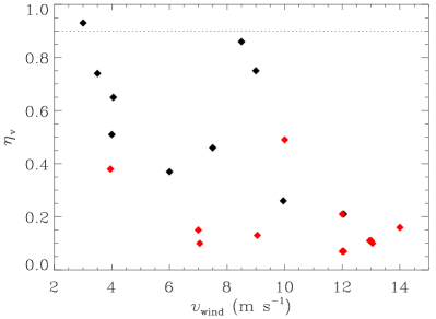
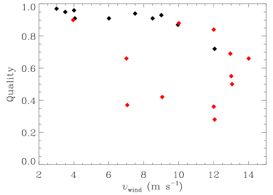
Figure 4: Phasing efficiency (top) and phasing quality (bottom) as a function of wind speed for the data sets presented in the current paper (Tables 1 & 2). Data sets with PWV$\geq$2.0 mm are indicated in red; data with PWV$<$2.0 mm are plotted in black. The horizontal dashed line in the upper panel indicates the nominal APS efficiency goal of $\geq$90%. All of the data sets plotted here were taken without the use of WVR-based fast phasing corrections.

To obtain a preliminary assessment of how the combination of wind speed and PWV affects phasing performance at 345 GHz, we plot in Figure 4 the phasing efficiency $\eta_{v}$ and the phasing quality as a function of wind speed $v_{\rm wind}$ for each of the data sets presented in the current paper (Tables 1 & 2). Data points with PWV$\geq$2.0 mm are shown in red and data with PWV$<$2.0 mm are shown in black.

Figure 4 shows that irrespective of wind speed, when PWV$>$2.0 mm, phasing efficiency in Band 7 generally falls below $\sim$50%. Thus operation of the APS in Band 7 in conditions with PWV$>$2.0 mm is not recommended in general, although it may be possible to relax this restriction with future use of the fast phasing mode (see above).

We also see in Figure 4 that when wind speeds exceed $\sim$10 m s^-1, phasing efficiency is consistently quite low ( $<$$\sim$20%), even in one case with PWV$<$2 mm. Furthermore, phasing solution quality is seen to decline systematically for such high wind speeds. This suggests that for the high wind-speed regime, the use of fast phasing corrections is unlikely to improve the overall phasing performance. It is thus recommended that phased array observations in Band 7 are strictly avoided in conditions with $v_{\rm wind}>$10 m s^-1.

For intermediate wind speeds ($3\leq v_{\rm wind}<10$ m s^-1) the situation is more complex. We find that (in absence of fast phasing corrections) one generally does not meet the nominal APS efficiency goal of $\eta_{v}\geq$0.9. However, for VLBI, the sensitivity and strategic importance of phased ALMA mean that even data with lower phasing efficiency may be scientifically useful. For example, when PWV is low ($<$2.0 mm), in many cases $\eta_{v}~{}\hbox to0.0pt{$>$\hss}{\lower 4.30554pt\hbox{$\sim$}}$0.5; assuming 37 phased 12 m antennas, this still provides the sensitivity comparable to a 25 m diameter parabolic dish. Furthermore, the generally good phasing quality seen for data sets with $3\leq v_{\rm wind}<10$ m s^-1 and PWV$\leq$2.0 mm suggests that the fraction of experiments achieving $\eta_{v}>$0.5 under this combination of conditions is expected to grow significantly with the use of the fast phasing mode. We are currently in the process of acquiring additional regression test data to explore how much improvement the fast mode provides under a range of observing conditions, including moderate wind speeds ($<$10 m s^-1) and moderate PWV values ($\sim$2–3 mm).

4.2 Impact of Array Size and Maximum Baseline Length

Table 6: Comparison of phase RMS as a function of baseline length.

Data set	Max. baseline	Date	Target	Flux	Phase RMS	Phase RMS
				density	all baselines	baselines$<$200 m
	(m)	(YYYY MMM DD)		(Jy)	(deg)	(deg)
B180	180	2015 Mar 30	3C273	4.0	16	16
B1500	1500	2015 Aug 02	J0522–3627	4.5	69	35
B6900	6900	2021 Sep 03	J1924–2914	3.0	55	39

Figure 5 compares phase as a function of $uv$ distance for two tests carried out in 2015 (on March 30 and August 2), and one carried out in 2021 (on September 3). The tests were taken under similar weather conditions (PWV$\sim$0.5 mm) but with different baselines ranges ($<$180 m, $<$1500 m, and $<$6900 m, respectively). Table 6 provides a summary of these tests, labelled B180, B1500, and B6900, respectively.

Considering the single correlation quadrant (SPW=0) and polarization (XX) that is plotted for each data set, we find that the RMS dispersion in the phases for all baselines in the phased array is significantly higher in the B1500 data (69 deg) and the B6900 data (55 deg) compared with the B180 data (16 deg). This is true even if we limit our comparison to baselines $<$200 m for all three data sets; in this case the RMS phase dispersions are 35 deg (B1500), 39 deg (B6900) and 16 deg (B180). We thus see evidence that even under relatively good weather conditions it is advantageous to limit the phased array to short baselines (less than a few hundred meters) when observing at wavelengths $\lambda~{}\hbox to0.0pt{$<$\hss}{\lower 4.30554pt\hbox{$\sim$}}$1 mm. Because the correlated amplitude scales as e${}^{-\sigma_{p}^{2}/2}$ where $\sigma_{p}$ is the RMS dispersion (in radians) of the phase, the sensitivity gained by the inclusion of antennas on long baselines will be significantly diminished by an overall decrease in phasing efficiency of the entire phased array. This can be understood as a result of the fact that the APS phase solver uses a least-squares method to convert baseline phases to station phases, and too many noisy baselines (typically those longer than a few hundred meters) will impact the overall quality of the phasing solutions.

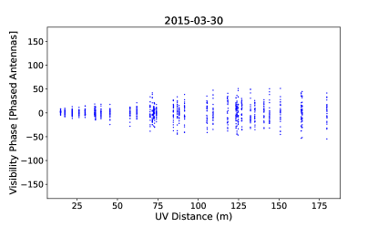
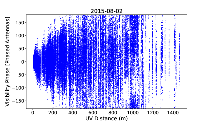
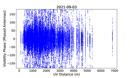
Figure 5: Phase (in degrees) as a function of projected baseline length (in meters) for Band 7 phasing tests on 2015 March 30 (top), 2015 August 2 (middle), and 2021 September 3 (bottom). In each case the target flux density is a few Jy (see text for details). The tests were taken under similar weather conditions (see Table 2). The mean RMS dispersions in the phases in the 2015 August and 2021 September data (with longest baselines $<$1.5 km and $<$6.9 km, respectively) are larger than in the 2015 March data where the longest baselines $<$0.2 km, even on the shortest baselines. Data from a single correlator quadrant (SPW=0, averaged over all channels) and a single polarization (XX) are shown in all panels. The phased array for the 2015 August observations included a number of 7 m CM antennas which are typically not included in the phased array (see Section 2.2.2).

4.3 Comparison between Band 6 and Band 7

To begin to assess how the performance of the APS in Band 7 compares with Band 6, we have performed preliminary analysis of test observations where Band 6 and Band 7 measurements were obtained within a single session. In particular, during the 2017 February 1 ALMA-only test and the 2018 October 18 VLBI test, data in both Bands 6 and 7 were acquired using comparable arrays, with baseline lengths ranging from $\sim$15 m to $\sim$300 m, while the PWV content varied in the range $\sim$1.5–2.0 mm.

To explore the relative performance in the two bands, in Figure 6 we compare the results from scans of a few minutes duration on the source J0522–3627 in each band, acquired on 2017 February 1. The RMS phase fluctuations for all phased baselines were 43 deg in Band 6 and 36 deg in Band 7. These relatively high phase dispersions reflect the sub-optimal weather conditions for observing in these bands (PWV$\sim$ 1.6 mm; wind speed $\sim$9 m s^-1), but these results nonetheless indicate that the phasing system is capable of comparable performance in Band 7 compared with Band 6. In this example, the fluctuations are actually slightly lower in Band 7 relative to Band 6. However, as the observations we compare here were not co-temporal, those differences can be ascribed to changes in PWV, coupled with changes in the source elevation. We reach similar conclusions from a preliminary analysis on the 2018 test dataset.

Our initial results suggest that for compact array sizes (baselines $\lesssim$300 m) and moderately good or better observing conditions (PWV $\lesssim$2 mm), high-quality and high-efficiency phased array performance will be possible in both Bands 6 and 7 and that Band 7 does not show any appreciable loss in phasing performance compared with Band 6. Under conditions where the phase fluctuations are dominated by tropospheric water vapor, some degradation in Band 7 performance compared with Band 6 is naturally expected to occur as a consequence of the linear wavelength dependence in the temporal phase fluctuations (e.g., Rioja et al., 2012) and the slightly lower aperture efficiency of the ALMA antennas in Band 7 compared with Band 6 (Remijan et al., 2019). However, in practice, we did not see any clear evidence of systematic degradation in phasing performance in Band 7, in part because only limited comparison data are available to date, and also because such comparisons are complicated by the modest variations in weather conditions that typically occur over tens of minutes during available test periods at ALMA.

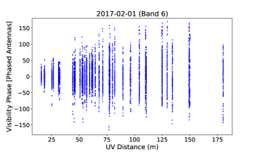
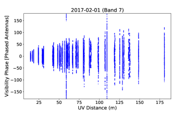
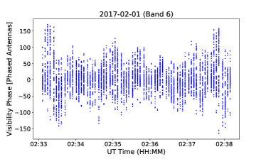
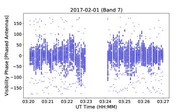
Figure 6: Phase (in degrees) as a function of projected baseline length in meters (upper panels) and observing time (lower panels) during scans of a few minutes duration on the source J0522–3627 using the APS on 2017 February 1 in Band 6 (left) and Band 7 (right), respectively, under conditions with PWV$\sim$1.6 mm and wind speeds of $\sim$9 m s^-1. The RMS phase fluctuations are $\sim$43 deg in Band 6 and $\sim$36 deg in Band 7, respectively, indicating comparable phasing performance in the two bands.

5 Additional Assessments of Phased Array Data Quality

The primary goal of phasing ALMA in Band 7 is to harness the enormous sensitivity and collecting area of ALMA for use a sub-mm VLBI station (e.g., Fish et al., 2013). This will be discussed further in Paper II. A key part of the process of turning the phased ALMA array into a functional sub-mm VLBI station will be to first calibrate the interferometric visibilities (Goddi et al., 2019). Because the data taken during the 2018 October VLBI test were intended for testing and engineering purposes only, a full suite of calibrators was not observed. However, as described in Appendix A, we have been able to perform a modified calibration scheme to the data to allow these data to be meaningfully combined with other VLBI stations (Paper II). This calibration scheme additionally allows us to perform some further quality assurance checks, as described below.

5.1 Accuracy of the Absolute Flux-density Scale

To assess the accuracy of the flux density calibration in VLBI mode, Goddi et al. (2019) compared the measured flux densities of VLBI targets with values derived from the independent flux monitoring done with the ACA, taking advantage of the fact that some of the Grid Sources are also observed in VLBI observations. The analysis in Goddi et al. (2019) showed that the flux density values estimated from ALMA during VLBI observations are generally within 5% in Band 3 and 10% in Band 6 when compared with the Grid Sources monitoring values (consistent with the expected absolute flux calibration uncertainty at ALMA; see Remijan et al. 2019).

We have performed a similar analysis for the Grid Sources observed in Band 7. Table 5 reports the measured flux values (per SPW) for all sources observed in Band 7 during the 2018 October campaign along with the archival flux values for Grid Sources. The flux values of the VLBI sources are estimated in the uv-plane using the CASA task fluxscale, which adopts a point-source model (this assumption is valid since Grid Sources are unresolved on ALMA baselines). The expected flux density of Grid Sources at a given time and frequency are retrieved from the ALMA archive via the getALMAflux() function implemented in the CASA analysis utils. Table 5 also reports the time difference between the VLBI observations and the archival entry, $\Delta t_{S}$, which is $<$1 day for all sources (i.e. they were observed with the ACA within less than a day of the VLBI observations) except BL Lac. The nominal calibration uncertainty at ALMA in Band 7 is $\sim$10% (see ALMA Technical Handbook – Remijan et al. 2019), and most of our new flux density estimates are consistent with the archival values to within this range, with the exception of CTA102 (with a 16% lower flux) and J0522$-$3627 (with a 13% higher flux).

5.2 Interferometric Test Images

As an additional means of assessing the science readiness of the APS in Band 7, we have produced images of the VLBI targets from fully-calibrated ALMA interferometric visibilities (see Appendix A), following the same procedures outlined in Goddi et al. (2021). We show representative images in Figure 7. The images displayed cover an area slightly smaller than the primary beam of the ALMA antennas (18″ at 350 GHz) and have a synthesized beamsize of roughly 0$\hbox to0.0pt{.\hss}^{\prime\prime}$45. The correction for the attenuation of the primary beam is not applied to these maps.

We have conducted a series of quality-assurance self-consistency tests on these images. We first assessed that the images are consistent with unresolved point sources (as expected for the selected VLBI targets), indicating that they are not smeared by residual phase errors. We then established that the size determined from a Gaussian fit matches the size of the synthesized beam (within $<1$%) and the peak flux and integrated flux have the same value (within $<1$%), as expected for point-like sources. Finally we confirmed that the peak flux occurs exactly at the phase center. Besides these self-consistency checks, we also estimated source flux densities from the images (following the methods outlined in Goddi et al. 2021) and assessed that they are consistent with the values estimated in Table 5 (within $\lesssim$10% for sources observed on the 18th/19th and within $\lesssim$5% for sources observed on the 21st, respectively).

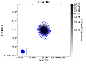
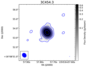
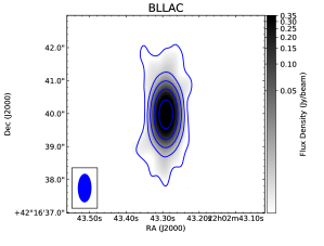
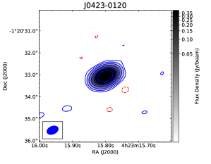
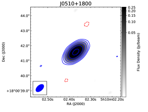
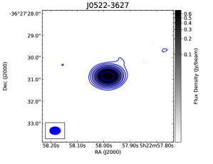
Figure 7: Representative total intensity images of targets observed during the 2018 October VLBI campaign. The grey-scale image shows emission at 347.6 GHz (SPW=2) while the blue contours show emission centered at 336.6 GHz (SPW=0); the red (dashed) contours indicate negative values. The contour levels are $\pm 3\sigma\times 2^{n}$ where $\sigma=$[0.9, 2.5, 0.7, 0.25, 0.27, 0.7] mJy beam^-1 for CTA 102, 3C454.3, BL Lac, J0423–0120, J0510+1800, J0522–3627, respectively, and $n=0\,,1\,,2\,,3\,\ldots$ up to the peak flux-density. The intensity brightness is plotted using a logarithmic weighting function (starting from the $3\sigma$-level). The major axis of the synthesized beam for BL Lac is $\sim$0$\hbox to0.0pt{.\hss}^{\prime\prime}$62 and for the remaining sources is 0$\hbox to0.0pt{.\hss}^{\prime\prime}$45-0$\hbox to0.0pt{.\hss}^{\prime\prime}$5.

6 Amplitude Calibration of Phased-ALMA as a Single VLBI Station

Traditionally VLBI stations store time-dependent amplitude corrections, $A(t)$, as a combination of $T_{\rm sys}$ (one value per intermediate frequency and integration time) and an instrumental gain given in degrees per flux unit (K/Jy) or DPFU (assumed to be stable over time and frequency):

$$A(t)=\sqrt{T_{\rm sys}/\mathrm{DPFU}}$$

In VLBI, one also often defines a system-equivalent flux density (SEFD) as the total system noise represented in units of equivalent incident flux density, which can be written as

$$\mathrm{SEFD}=\left<T_{\rm sys}\right>/\mathrm{DPFU}.$$ (1)

In the following, we estimate DPFU, $T_{\rm sys}$, and SEFD for phased-ALMA in Band 7 using the data collected on 2018 October 18/19 and 21. Representative values are reported in Table 7.

Table 7: ALMA Band 7 Antenna Parameters for Observations in 2018 October

Date	$N_{\rm phased}$	$T_{\rm sys}$a	DPFUb	$T_{\rm sys}$[sum]c	SEFDd
(2018 Oct.)	Ant.	(K)	(K/Jy)	(K)	(Jy)
Band 7
21	29	155	0.011	2.6	238
18/19	25	200	0.011	6.4	578
Band 6
19	25	80	0.006	0.9	150

6.1 DPFU

While in a single-dish telescope the DPFU is fixed, in a phased array it scales with the number of phased antennas. Because the number of phased antennas can change during the observations, the DPFU may also change. In order to keep the DPFU of phased ALMA constant over a given observation (for calibration purposes), we set the DPFU of phased ALMA to the antenna-wise average of DPFUs (instead of the antenna-wise sum). The DPFU of a single antenna $i$ is calculated using the measured $T_{\rm sys}$ and amplitude gains $g_{a,i}$ computed from self-calibration during QA2 (these are stored in the <label>.flux_inf.APP.OpCorr table; see Appendix B):

$${\rm DPFU}_{i}=\langle 1/g_{a,i}^{2}\rangle/\langle 1/T_{{\rm sys},i}\rangle$$ (2)

where the average $\langle$ $\rangle$ is computed over all scans where a $T_{\rm sys}$ is measured at the antenna $i$.

Using the data collected on October 21 (which have higher quality), we estimate DPFU = 0.011 K/Jy. We assume this value as the single-antenna average DPFU for Band 7 phased ALMA observations in 2018 October. The DPFU for a phased array of 29 antennas would be: (DPFU)₂₉ = 0.32 K/Jy.

6.2 T_sys and ANTAB files

The amplitude calibration for phased ALMA is computed via a linear interpolation of the ALMA antenna gains and it is stored in the “ANTAB” format. This is the standard file used in VLBI to store amplitude a-priori information, and readable by the Astronomical Image Processing System (AIPS) task ANTAB (Greisen, 2003).

The ANTAB files are generated directly from the antenna-wise average of all the amplitude gains $g_{a}$ and phase gains $g_{p}$ (stored in the QA2 <label>.flux_inf.OpCorr.APP and <label>.phase_int.APP tables, respectively; see Appendix B):

$$T_{\rm sys}=\frac{{\rm DPFU}}{\langle[g_{a}e^{ig_{p}}]^{2}\rangle}\frac{1}{N_{\rm phased}}$$ (3)

where the average $\langle$ $\rangle$ runs on all time integrations where gain solutions are found and on all phased antennas (see Eq. 16 in Goddi et al. 2019).

Using Eq. 3 and DPFU $=0.011$ K/Jy, one can derive an effective phased-array system temperature for each scan. These are shown in Figure 8 for 2018 October 18/19 and 21. Note that since we set the DPFU of phased-ALMA to the antenna-wise average of DPFUs, there is a factor of $N_{\rm phased}$ that must be absorbed by $T_{\rm sys}$ in order to keep the same amplitude correction. This explains why the plotted values (varying in the range $\sim$2-10 K) are much lower than the measured $T_{\rm sys}$  of the individual antennas in Band 7 ($\sim$100-300 K).

Note that the specification for the ALMA receiver noise performance is $\sim$80 K in Band 6 and $\sim$150 K in Band 7 (Remijan et al., 2019), very close to the median $T_{\rm sys}$ values measured on October 19 in Band 6 and on October 21 in Band 7, respectively; the much higher $T_{\rm sys}$ measured on the October 18/19 in Band 7 reflects the rapid changes in the weather conditions on that night (see Table 7).

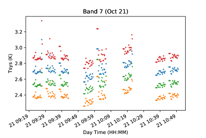
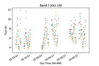
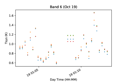
Figure 8: ANTAB $T_{\rm sys}$ values derived as described in Section 6.2 on October 21 (top) and 18/19 (middle) in Band 7 and October 19 in Band 6 (bottom). Note the much larger scatter and higher values of the $T_{\rm sys}$ computed on October 18/19 with respect to October 21. Colors display different SPWs. A DPFU=0.011Jy/K and 0.006 Jy/K is assumed in Band 7 and 6, respectively.

6.3 SEFD

Using Eq. 1, and plugging in the median of the phased-array $T_{\rm sys}$ values measured on October 21 (2.6 K) and the estimated DPFU (0.011 Jy/K), one derives SEFD = 238 Jy in Band 7. One can also compare this estimate with the theoretically expected SEFD_th as provided by the ALMA observatory:

$$\mathrm{SEFD}_{\rm th}=\frac{\left<T_{\rm sys}\right>\ 2k_{B}}{\eta_{A}A_{\rm geom}},$$ (4)

where $T_{\rm sys}$ is the opacity-corrected system temperature, $k_{B}$ is the Boltzmann constant, $\eta_{A}$ is the aperture efficiency, and $A_{\rm geom}$ is the geometric collecting area. For a 12 m ALMA dish in Band 7, $\eta_{A}$=0.63 (Remijan et al., 2019). Assuming a phased array of 29 antennas of 12 m diameter and taking a representative value of $T_{\rm sys}$= 155 K (corresponding to the mean value of the $T_{\rm sys}$measured on October 21), one derives SEFD_th = 207 Jy. Taking into account the phasing efficiency and defining $\mathrm{SEFD}=\mathrm{SEFD}_{\rm th}/\eta_{v}$, one finds SEFD = 230 Jy for 90% efficiency, close to the estimate from the QA2 gain calibration.

A similar analysis on the data acquired on October 18/19 provides SEFD = 150 Jy in Band 6 and SEFD = 578 Jy in Band 7. The latter is a factor of 2.4 higher than the value estimated on October 21, likely a consequence of the poor observing conditions.

7 Summary

This paper presents the first test observations of ALMA as a phased array at 345 GHz (Band 7). These include phased array data acquired during a series of short ALMA standalone tests and during a global VLBI test campaign conducted in 2018 October. We also present a description of the special procedures for calibration and a preliminary analysis of the ALMA observations aimed at validation of the Band 7 phased-array operations in VLBI mode.

We find that under nominal Band 7 observing conditions at ALMA (PWV $<$$\sim$2.0 mm; $v_{\rm wind}<$10 m s^-1), ALMA can perform as a scientifically effective phased array, with a phasing efficiency $\eta_{v}~{}\hbox to0.0pt{$>$\hss}{\lower 4.30554pt\hbox{$\sim$}}$0.5. Typical phasing efficiencies achieved under these conditions are expected to increase with future use of fast (WVR-based) phasing corrections in addition to the TelCal-based phasing corrections used in the present study. At 1.3 mm the order-of-magnitude boost in sensitivity of phased ALMA was crucial for enabling the first ever images of SgrA* and M87*. At 345 GHz, ALMA is now poised to provide a comparable leap in capabilities and serve as a vital anchor station for the first VLBI observations at submillimeter wavelengths. However, we find that phasing performance in Band 7 diminishes significantly during periods of high winds ( $>$$\sim$12 m s^-1) which should thus be avoided, even when PWV is low. Under high-wind conditions, the effective collecting area of the phased array may approach that of a single 12 m antenna. We also conclude that it is generally advantageous to limit the maximum baseline lengths in the phased array to a few hundred meters or less when operating in Band 7.

As will be described in Paper II, the phased ALMA data collected on October 18/19 and 21 led to the detection of the first VLBI fringes in the 345 GHz band between ALMA and other EHT sites. The detection of 345 GHz VLBI fringes represents a crucial first step, not only for commissioning sub-mm VLBI at ALMA, but in general for establishing that such measurements are both technically and practically feasible. Pushing the VLBI capability of phased-ALMA to the highest frequencies is crucial for the success of scientific experiments that require extremely high-angular resolution, including studies of black hole physics on event horizon scales and accretion and outflow processes around black holes in AGNs.

Appendix A Calibration of the 2018 VLBI Campaign Data

In order to turn the phased ALMA array into a single mm or sub-mm VLBI station and combine it with other VLBI stations (e.g. Paper II), it is necessary to first calibrate the interferometric visibilities (Goddi et al., 2019). Although the data sets described in this paper did not include the full suite of calibration measurements that would usually be part of an ALMA VLBI science observation, we were nonetheless able to perform some basic calibrations of the data sets from the 2018 October global Band 7 VLBI test campaign (Table 2) using a modified version of the procedure described in Goddi et al. (2019). The steps are outlined here.

In brief, we have calibrated the ALMA data using the Common Astronomy Software Applications (casa) package (CASA Team et al., 2022) and the special procedures known as “Quality Assurance Level 2” (QA2) described in Goddi et al. (2019). Normally VLBI observations are arranged and calibrated in “tracks”, where one track consists of the observations taken during the same day or session. Since the observations carried out during each night were insufficient to allow for their independent calibration, we concatenated the data collected in 2018 October into a single dataset. In addition, since the poor weather conditions made the data collected on days 16 and 17 unusable (see Section 4), we flagged them from the concatenated dataset. We have therefore based our analysis on the data collected on days 18/19 and 21; the latter yielded the highest-quality data and were used to compute the bandpass and polarization calibration tables (see Appendix B). We then applied those calibration tables to the full dataset, under the assumption that the observed sources are stable over a time interval of 2.5 days.

A.1 Absolute Flux-density Scale

ALMA normally tracks the atmospheric opacity by measuring system temperatures ($T_{\rm sys}$) at each antenna. However, $T_{\rm sys}$  values are not used in the phased-array data calibration to avoid biasing the calibration of the phased sum antenna (see Goddi et al., 2019). While the bulk of the opacity effects are removed with self-calibration, $T_{\rm sys}$ (usually measured a few times per hour) can still be used to correct for second-order opacity effects, related to the difference between the opacity correction in the observation of the primary flux calibrator and the (average) opacity in the observation of any given source.

In Goddi et al. (2019) the opacity-corrected flux density $S^{S}_{\tau}$ for a given source $S$ was estimated post-QA2 calibration by computing the products of the antenna-wise average of the amplitude gains, $g_{a}^{S}(t)$, times the antenna-wise average of valid $T_{\rm sys}$ measurements, $T^{S}_{\rm sys}(t)$, and then taking the ratio between a given source S and the primary flux-density calibrator P such as:

$$S^{S}_{\tau}=\left(\frac{\left<g_{a}^{S}(t)T^{S}_{\rm sys}(t)\right>}{\left<g_{a}^{P}(t)T^{P}_{\rm sys}(t)\right>}\right)^{2}S^{S}_{QA2}$$ (A1)

Here we have followed a similar approach, except that the opacity correction is applied to the data right after the gain calibration, yielding opacity-corrected amplitude gains (contained in the <label>.flux_inf.APP.OpCorr table in the ALMA archive).

The absolute flux-density scale was derived from self-calibration on 3C454.3. This quasar was chosen as the primary flux-density calibrator because it is the only Grid Source observed in both Bands 6 and 7, allowing calibration of the amplitude scale in both bands. For this purpose, $S^{P}_{343GHz}=3.53$ Jy and $\alpha$=–0.69 was assumed. See Section 5.1 for an assessment of the accuracy of the absolute flux-density scale.

A.2 Polarization Calibration

Obtaining accurately calibrated VLBI science data from ALMA requires a full polarization calibration of the interferometric visibilities to allow conversion of ALMA’s linearly polarized data products to a circular polarization basis, for consistency with other VLBI stations (Martí-Vidal et al., 2016; Matthews et al., 2018; Goddi et al., 2019). Observations of a polarization calibrator with sufficient parallactic angle coverage are required to simultaneously derive a reliable model of the polarization calibrator and an estimate of the XY cross-phase at the reference antenna. The latter is computed by running the CASA task gaincal in mode XYf+QU (see §5.2.3 of Goddi et al., 2019).

Since the 2018 October campaign was conceived as a VLBI “fringe test”, it was not designed to obtain fully calibrated science data from ALMA and, consequently, no frequent observations of a suitable polarization calibrator were obtained. Instead, only a few scans were obtained towards two sources with a high linear polarization fraction ($\gtrsim$5%), J0522–3627 and J0510+1800 (see Table 3). This precluded deriving a reliable polarization model from the observations using gaincal. Fortunately, both sources were observed with the ACA in Band 7 on October 10 and October 21/22 and we could estimate their Stokes parameters using the AMAPOLA polarimetric Grid Sources. We set J0510+1800 as the polarization calibrator and its Stokes parameters as IQUV = [1.28, –0.134, 0.079, 0.0] Jy (see Appendix D for an assessment of the goodness of the polarization model). We then ran the CASA task polcal in mode Xf to estimate the XY phase at the reference antenna.

The computed cross-hand phases as a function of frequency are plotted in Figure 9. The four left panels reveal a steep phase slope with frequency, which indicates the presence of a significant cross-hand delay ($>$0.5 nanoseconds or a full wrap within the $\sim$2 GHz SPW) intrinsic to the reference antenna.

This can be a consequence of two factors. First, the gain and bandpass calibration only correct for parallel-hand delay residuals (the two polarizations are referenced independently), thus leaving a single cross-hand delay residual from the reference antenna. Second, the online system does not apply the static baseband delay corrections when the APS is active (Matthews et al., 2018). In general, the phasing corrections applied to contiguous frequency chunks are expected to remove most of the (generally large) baseband delays. (This was previously demonstrated in science observations carried out in Band 3 and Band 6; see Goddi et al. 2019). Despite this, a significant residual delay in the XY cross-phases may still be present, depending on the nature of the observations, as demonstrated in this case. This cross-hand delay can be estimated with gaincal using gaintype=‘KCROSS’. We therefore included this additional correction with respect to the procedures outlined in Section 5 of Goddi et al. (2019). Figure 9 (right panels) shows plots of cross-hand phases after removing the cross-hand delay, which indeed reveal a flat slope with frequency.

We explicitly note that the approach to polarization calibration outlined above could be useful in future cases where no suitable polarization calibration is observed, or only short VLBI observations can be obtained because of weather or scheduling constraints.

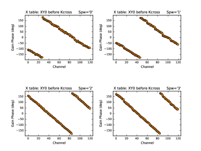
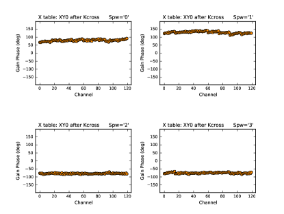
Figure 9: X-Y cross-phase of the reference antenna in APS mode for each of the four SPWs before (left) and after (right) removing the cross-polarization phase delay.

Appendix B Validation of the APS Calibration

The QA2 data calibration presented in Appendix A provides a full set of calibration tables in Measurement Set format (i.e. readable in CASA):

• <label>.CSV.phase_int.APP.XYsmooth: phase gains (per integration time).

• <label>.CSV.flux_inf.APP.OpCorr: amplitude gains scaled to Jy units (per scan).

• <label>.CSV.bandpass_zphs: bandpass (with zeroed phases).

• <label>.CSV.XY0.APP: cross-polarization phase at the TelCal phasing reference antenna.

• <label>.CSV.Kcrs.APP: cross-polarization phase delay at the TelCal phasing reference antenna (see Appendix D).

• <label>.CSV.Gxyamp.APP: amplitude cross-polarization ratios for all antennas.

• <label>.CSV.Df0.APP: D-terms at all antennas.

These tables can be used to fully calibrate the ALMA interferometric visibilities, which in turn can be used to do science analysis, e.g. deriving the mm emission properties of the VLBI targets such as integrated fluxes (see Section 5.1), or imaging them on arcsecond-scales (see Section 5.2). The same tables can also be processed to calibrate phased-ALMA as a single VLBI station (see Paper II).

Appendix C Weather Metrics

Figure 10 illustrates the weather conditions during the 345 GHz (Band 7) VLBI experiment on 2018 October. The left and right panels show PWV column in mm and the wind speed in m s^-1, respectively, as a function of observing time. Different rows show different days, from October 16 to October 21 (top to bottom).

At the beginning of the campaign (on the night of October 16/17 and the morning of October 17, respectively), the conditions on the Chajnantor Plateau were extremely unstable, with moderately high and variable PWV ($\sim 2\pm 0.3$ and $1.8\pm 0.8$ mm) and high wind speeds ($\sim 9\pm 5$ m s^-1 and $\sim 12\pm 4$ m s^-1) compared with typical conditions at ALMA for Band 7 observing. Atmospheric stability was significantly improved on the night of the 18/19 (PWV$\sim 1.1\pm 0.3$ mm) but wind speed was still significant ($\sim 6\pm 4$ m s^-1). On the last day of observing (October 21) weather at ALMA was excellent, with PWV$\sim 0.8\pm 0.1$ mm and wind speed of $\sim 3\pm 3$ m s^-1.

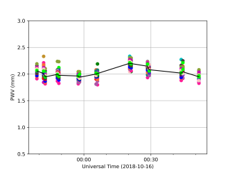
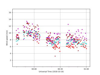
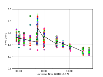
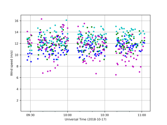
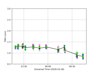
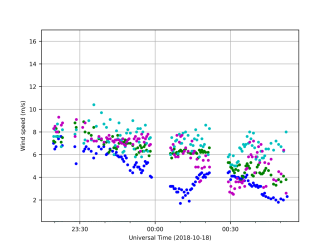
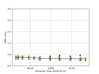
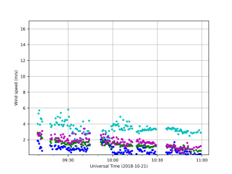
Figure 10: Illustration of the weather conditions during the 345 GHz (Band 7) VLBI test experiment on 2018 October 16/17, 17, 18/19, 21 (from top to bottom). Left panels: PWV column in mm as a function of observing time. Colors display different antennas. The black line is the median PWV value computed across all antennas in the array. Right panels: wind speed in m s^-1 as a function of observing time. Colors indicate data from different weather monitoring stations.

Appendix D Assessment of the Polarization Calibration model used for the October 2018 VLBI test

To evaluate the goodness of the AMAPOLA model for J0510+1800, we ran the CASA task polcal with different input models. The latter included deviations in either the linearly polarized flux, $P=\sqrt{Q^{2}+U^{2}}$, or polarization position angle, $2\chi=\mathrm{arctan}(U/Q)$, with respect to the AMAPOLA model (with $P_{\rm amapola}=0.16$ Jy and $\chi_{\rm amapola}=75^{\circ}$). In particular, we considered the following 17 alternative models: $P=\Delta P\times P_{\rm amapola}$ where $\Delta P=$ [0.25, 0.50,0.75,1.25,1.50,1.75,2.00] (these models kept the same $U/Q$ ratio) and $\chi=\chi_{\rm amapola}\pm\Delta{\chi}$ where $\Delta{\chi}=\pm[10,20,30,40,50]$deg.

We then assessed the impact of different models on the D-terms of the phased-antennas. To this end, we computed the D-terms “channel dispersion”, a parameter defined by the range (minimum to maximum) of the average of the D-terms (absolute) values computed across all antennas for each channel. Figure 11 summarizes the values of this parameter for the class of models presented above. We found that deviations from the AMAPOLA model always resulted in a deterioration of the D-terms of the phased-antennas, with a monotonically increase in the D-term dispersions (typically a factor of few higher than the original model). This simple analysis provides an a-posteriori validation of the polarization model assumed to perform the interferometric data calibration.

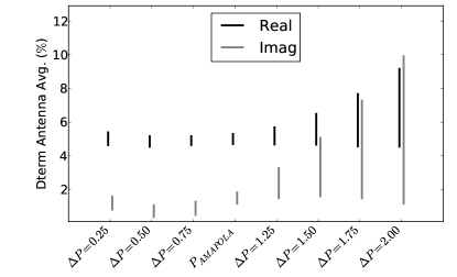
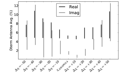
Figure 11: Left panel: Impact of the deviations from the J0510+1800 AMAPOLA model on the D-terms of the phased-antennas. Models including deviations in the polarized flux: $P=\Delta P\times P_{\rm amapola}$ (where $P_{\rm amapola}=0.16$ Jy). Right panel: Models including deviations in the polarization position angle: $\chi=\chi_{\rm amapola}\pm\Delta{\chi}$ (where $\chi_{\rm amapola}=75^{\circ}$).

Appendix E Concerning Phasing Efficiency

Here we provide some remarks on the characterization of phasing efficiency, which is used as a key metric in the current paper for evaluating the APS performance in Band 7.

As described in Matthews et al. (2018), for an idealized phased array, a phasing efficiency, $\eta_{p}$, can be defined as a function of the cross-correlation between the summed signal and that of a comparison antenna, divided by the averaged cross-correlations between the comparison antenna and the individual phased elements:

$$\eta_{p}\equiv\frac{\left<V_{\rm sum}V_{c}\right>}{\left<V_{i}V_{c}\right>}\frac{1}{\sqrt{N_{\rm phased}}}.$$ (E1)

Here $N_{\rm phased}$ is the number of phased antennas.

In principle, monitoring $\eta_{p}$ during an observation can provide a fundamental figure-of-merit to characterize the performance of the phasing system. To meet the need for a readily computable efficiency metric, the APS was designed to include the ability to substitute one antenna input to the ALMA Baseline Correlator with a copy of the phased-sum signal. The correlator then produces visibilities on baselines to this “sum antenna”, allowing it to be analyzed by the online system in a manner analogous to the real antennas comprising the ALMA array. This system was modeled after the PhRInGES software previously used at the Submillimeter Array (SMA; J. Weintroub, private communication). Figure 3, discussed in the main text, shows examples of plots of phase and correlated amplitude, respectively, as a function of time for baselines to this sum antenna. As described in the main text, such plots allow useful qualitative assessment of the phasing performance.

By definition, a perfectly phased array will have $\eta_{p}=1$ and deviations from this ideal can then be used to characterize efficiency losses. In a real-world system, such efficiency losses occur from multiple effects, including imperfections in the phasing solutions (e.g., due to rapid atmospheric phase fluctuations and/or time lags in the application of the phasing solutions), non-optimized antenna weighting in the phased sum, and inherent losses due to quantization effects and other properties of signal chain and hardware (Crew, G. & Matthews, L., 2015).

As discussed in Matthews et al. (2018), under optimal weather conditions the end-to-end efficiency of the APS as defined by Eq. E1 has been found to be $\sim$60% of an ideal system in Bands 3 and 6 ($\eta_{p}\sim$0.6). Portions of these efficiency losses result from known effects, including the two-bit quantization of the phased sum signal, residual delay errors, and the neglect of antenna-based weighting factors in computing the phased sum. However, approximately 20% of this efficiency loss remained unaccounted for. Subsequent investigation has now uncovered the source of this additional loss; specifically, because the logic that computes the sum signal in the APS is significantly slower than originally designed, it arrives with a 24-lag delay (192 ns). In a 128 lag design, this results in a loss factor of [$(128-24)/128=0.8125$], i.e., $\sim$20% in correlated amplitude.

Because certain efficiency losses in any phasing system, including the aforementioned 24-lag delay, are essentially fixed and unvarying, it is useful to decouple these from losses in efficiency that result from time-varying phenomena (e.g., weather; baseline length, etc.), as the latter may be used to inform real-time adjustments to the observing strategy and/or phased array parameters (e.g., changes in selection of antennas within the phased array or termination of a phased array observation because of poor phasing stability). This need has led us to define and compute (in ALMA’s TelCal software) an alternate phasing efficiency metric, $\eta_{v}$:

$$\eta_{v}~{}=~{}{{\sum_{ij}{v_{ij}}}\over{\sum_{ij}{|v_{ij}|}}}$$ (E2)

Here $v_{ij}$ is the visibility on the baseline between antennas $i$ and $j$ of the $N$ phased array antennas. This manner of defining phasing efficiency is similar to the approach adopted in the SMA SWARM correlator (Young, A. et al., 2016). During observations, $\eta_{v}$ provides a useful quantitative, real-time metric of phasing efficiency. Because this definition is not computed based on the phased sum signal, it is free from losses due to quantization and the 24-lag delay. We therefore quote $\eta_{v}$ as a metric of phasing efficiency throughout the discussions of phasing performance in the main text. In contrast, we limit the use of the phasing efficiency, $\eta_{p}$ defined by Eq. E1 (computed using baselines to the APS phased sum “antenna”) only for qualitative evaluation (e.g., Figure 3 of the main text). We note that the original design requirements of the APS specified that under band-appropriate observing conditions, the system should routinely achieve $\eta_{v}\geq$0.9 in Bands 3 and 6 (Matthews et al., 2018). However, in practice, under excellent weather conditions we find $\eta_{v}\rightarrow$1, even in Band 7.

During VLBI observations, the calculation in Eq. E2 is repeated during the polarization conversion (PolConvert) process that converts ALMA’s linearly polarized data products to a circular basis (see Section 7 in Matthews et al. 2018). This allows recovery of the correct amplitude scaling of the VLBI products for use in the ANTAB tables (Goddi et al., 2019).

References

- CASA Team et al. (2022) CASA Team, Bean, B., Bhatnagar, S., et al. 2022, PASP, 134, 114501
- Crew, G. & Matthews, L. (2015) Crew, G., & Matthews, L. 2015, ALMA Phasing Project Phasing Efficiency Status Report, ALMA Memo ALMA-05.11.63.03-0001-A-REP, ,
- Doeleman (2010) Doeleman, S. 2010, in 10th European VLBI Network Symposium and EVN Users Meeting: VLBI and the New Generation of Radio Arrays, Vol. 10, 53
- Doeleman et al. (2011) Doeleman, S., Mai, T., Rogers, A. E. E., et al. 2011, PASP, 123, 582
- Doeleman et al. (2009) Doeleman, S., Agol, E., Backer, D., et al. 2009, in astro2010: The Astronomy and Astrophysics Decadal Survey, Vol. 2010, 68
- Event Horizon Telescope Collaboration et al. (2019a) Event Horizon Telescope Collaboration, Akiyama, K., Alberdi, A., et al. 2019a, ApJ, 875, L1
- Event Horizon Telescope Collaboration et al. (2019b) —. 2019b, ApJ, 875, L2
- Event Horizon Telescope Collaboration et al. (2019c) —. 2019c, ApJ, 875, L3
- Event Horizon Telescope Collaboration et al. (2019d) —. 2019d, ApJ, 875, L4
- Event Horizon Telescope Collaboration et al. (2019e) —. 2019e, ApJ, 875, L6
- Event Horizon Telescope Collaboration et al. (2019f) —. 2019f, ApJ, 875, L5
- Event Horizon Telescope Collaboration et al. (2022a) —. 2022a, ApJ, 930, L12
- Event Horizon Telescope Collaboration et al. (2022b) —. 2022b, ApJ, 930, L13
- Event Horizon Telescope Collaboration et al. (2022c) —. 2022c, ApJ, 930, L14
- Event Horizon Telescope Collaboration et al. (2022d) —. 2022d, ApJ, 930, L15
- Event Horizon Telescope Collaboration et al. (2022e) —. 2022e, ApJ, 930, L16
- Event Horizon Telescope Collaboration et al. (2022f) —. 2022f, ApJ, 930, L17
- Event Horizon Telescope Collaboration et al. (2022g) —. 2022g, ApJ, 930, L14
- Falcke et al. (2001) Falcke, H., Markoff, S., Biermann, P. L., et al. 2001, in IAU Symposium, Vol. 205, Galaxies and their Constituents at the Highest Angular Resolutions, ed. R. T. Schilizzi, 28
- Fish et al. (2013) Fish, V., Alef, W., Anderson, J., et al. 2013, arXiv e-prints, arXiv:1309.3519
- Goddi et al. (2019) Goddi, C., Martí-Vidal, I., Messias, H., et al. 2019, PASP, 131, 075003
- Goddi et al. (2021) —. 2021, ApJ, 910, L14
- Greisen (2003) Greisen, E. W. 2003, in Astrophysics and Space Science Library, Vol. 285, Information Handling in Astronomy - Historical Vistas, ed. A. Heck, 109
- Issaoun et al. (2019) Issaoun, S., Johnson, M. D., Blackburn, L., et al. 2019, ApJ, 871, 30
- Johnson (2016) Johnson, M. D. 2016, ApJ, 833, 74
- Johnson & Gwinn (2015) Johnson, M. D., & Gwinn, C. R. 2015, ApJ, 805, 180
- Krichbaum et al. (2008) Krichbaum, T. P., Bach, U., Graham, D. A., et al. 2008, arXiv e-prints, arXiv:0812.4211
- Liu et al. (2019) Liu, K., Young, A., Wharton, R., et al. 2019, ApJ, 885, L10
- Liu et al. (2021) Liu, K., Desvignes, G., Eatough, R. P., et al. 2021, ApJ, 914, 30
- Martí-Vidal et al. (2016) Martí-Vidal, I., Roy, A., Conway, J., & Zensus, A. J. 2016, A&A, 587, A143
- Matsushita et al. (2017) Matsushita, S., Asaki, Y., Fomalont, E. B., et al. 2017, PASP, 129, 035004
- Matthews et al. (2018) Matthews, L. D., Crew, G. B., Doeleman, S. S., et al. 2018, PASP, 130, 015002
- Maud et al. (2017) Maud, L. T., Tilanus, R. P. J., van Kempen, T. A., et al. 2017, A&A, 605, A121
- Miyoshi & Kameno (2002) Miyoshi, M., & Kameno, S. 2002, in International VLBI Service for Geodesy and Astrometry: General Meeting Proceedings, ed. N. R. Vandenberg & K. D. Baver, 199
- Nikolic et al. (2013) Nikolic, B., Bolton, R. C., Graves, S. F., Hills, R. E., & Richer, J. S. 2013, A&A, 552, A104
- Primiani et al. (2016) Primiani, R. A., Young, K. H., Young, A., et al. 2016, J. of Astron. Instr., 05, 1641006
- Remijan et al. (2019) Remijan, A., Biggs, A., Cortes, P., et al. 2019, ALMA Technical Handbook
- Rioja et al. (2012) Rioja, M., Dodson, R., Asaki, Y., Hartnett, J., & Tingay, S. 2012, AJ, 144, 121
- Smith et al. (2000) Smith, D. R., Paglione, T. A., Lovell, A. J., Ukita, N., & Matsuo, H. 2000, in Society of Photo-Optical Instrumentation Engineers (SPIE) Conference Series, Vol. 4015, Radio Telescopes, ed. H. R. Butcher, 467–475
- Thompson et al. (2017) Thompson, A. R., Moran, J. M., & Swenson, George W., J. 2017, Interferometry and Synthesis in Radio Astronomy, 3rd Edition, doi:10.1007/978-3-319-44431-4
- Weintroub (2008) Weintroub, J. 2008, in Journal of Physics Conference Series, Vol. 131, Journal of Physics Conference Series, 012047
- Young, A. et al. (2016) Young, A., Primiani, R., Weintroub, J., et al. 2016, in Phased Array Systems and Technology (ARRAY), 2016 IEEE International Symposium on, 18-21 Oct. 2016