Fast and Reliable Jackknife and Bootstrap
Methods for Cluster-Robust Inference

Abstract

We provide computationally attractive methods to obtain jackknife-based cluster-robust variance matrix estimators (CRVEs) for linear regression models estimated by least squares. We also propose several new variants of the wild cluster bootstrap, which involve these CRVEs, jackknife-based bootstrap data-generating processes, or both. Extensive simulation experiments suggest that the new methods can provide much more reliable inferences than existing ones in cases where the latter are not trustworthy, such as when the number of clusters is small and/or cluster sizes vary substantially. Three empirical examples illustrate the new methods.

Keywords: clustered data, grouped data, cluster-robust variance estimator, CRVE, cluster sizes, wild cluster bootstrap

JEL Codes: C10, C12, C21, C23.

1 Introduction

In applications of linear regression models to many fields of economics and other disciplines, it is common to divide the sample into disjoint clusters and employ a cluster-robust variance matrix estimator (or CRVE) for inference. These estimators are based on the assumption that the disturbances of the regression model are uncorrelated across clusters, but they allow for arbitrary patterns of dependence and heteroskedasticity within each cluster. The literature on cluster-robust inference has grown rapidly in recent years. Cameron and Miller (2015) is a classic survey article. Conley, Gonçalves and Hansen (2018) surveys a broader class of methods for dependent data. MacKinnon, Nielsen and Webb (2023) provides a guide that explores the implications of key theoretical results for empirical practice, with an emphasis on bootstrap methods.

There are several CRVEs for ordinary least squares (OLS) estimates of linear regression models; see Section 2. However, because the one known as CV₁ is easy to compute and is the default in Stata, almost all empirical work to date has used it. Cluster-robust tests and confidence intervals based on CV₁ may or may not yield reliable inferences. Whether they do so depends primarily on the number of clusters $G$ and how homogeneous these are. When all clusters are roughly equal in size and approximately balanced, asymptotic inference based on CV₁ seems to be fairly reliable whenever $G$ is at least moderately large (say 50 or more). However, even when $G$ is very large, cluster-robust $t$-tests and Wald tests are at risk of severe over-rejection, and cluster-robust confidence intervals are at risk of severe under-coverage in at least two situations. The first is when one or a few clusters are much larger than the rest, and the second is when the only “treated” observations belong to just a few clusters; Djogbenou, MacKinnon and Nielsen (2019) discusses the first case, and MacKinnon and Webb (2017, 2018) discuss the second.

Alternatives to CV₁ have been known since Bell and McCaffrey (2002). The first contribution of the present paper, which is discussed in Section 3, is to provide a fast method for computing jackknife-based CRVEs, of which the simplest is generally known as CV₃. By explicitly using the cluster jackknife for computation in an efficient way, our method makes it feasible to employ CV₃ for inference even in very large samples with a large number of clusters.

Because CV₃ standard errors used to be hard to compute, there has been very little work comparing the finite-sample performance of $t$-tests based on CV₃ with those of similar procedures based on CV₁; a partial exception is Niccodemi and Wansbeek (2022). The second contribution of this paper is to compare the finite-sample properties of these tests, and also ones based on CV₂, by simulation; see Section 6. In concurrent work that cites our simulations, Hansen (2022) provides important theoretical results which suggest that asymptotic inference based on CV₃ is generally more reliable, and more conservative, than asymptotic inference based on CV₁.

Existing bootstrap methods for cluster-robust inference are all based on CV₁. The best known of these (and until now the best performing one) seems to be the wild cluster restricted (or WCR) bootstrap proposed in Cameron, Gelbach and Miller (2008). There is also a closely related procedure called the wild cluster unrestricted (or WCU) bootstrap, which generally does not work quite as well. The asymptotic validity of these procedures is proved in Djogbenou et al. (2019), which also analyzes their higher-order asymptotic properties. Until a few years ago, the WCR and WCU bootstraps were computationally expensive for large samples, but that is no longer the case. Roodman, MacKinnon, Nielsen and Webb (2019) describes a remarkably efficient implementation in the Stata package boottest, and MacKinnon (2022) discusses other methods for fast computation. The boottest routines are now available as a Julia package which can be also be called from R, Python, and Stata. The package fwildclusterboot implements the boottest method natively in R (Fischer and Roodman, 2022).

The third contribution of this paper is to propose several new variants of the wild cluster bootstrap. One modification simply replaces CV₁ by CV₃. The other, which requires some new results, involves modifying the bootstrap data-generating process, or DGP. Modern treatments of the wild cluster bootstrap, such as MacKinnon et al. (2023), express the bootstrap DGP as a function of the empirical scores. We show how to make the bootstrap DGP more closely resemble the (unknown) true DGP by transforming the residuals before forming the scores. The transformation we propose is based on the jackknife. Accordingly, it does not actually require any calculations that explicitly involve residuals. This makes it very fast when the number of clusters is small relative to the sample size, even when the latter is extremely large.

The next section establishes notation and briefly reviews the literature on asymptotic cluster-robust inference for the linear regression model. Section 3 then discusses a computational method for CV₃ which is conceptually simple and extremely fast in many cases, as we demonstrate in Section 4. Next, Section 5 discusses several ways of modifying the wild cluster bootstrap. Simulation results in Section 6 suggest that our new versions of the WCR and WCU bootstraps perform better, sometimes very much better, than the original ones. This is particularly true when cluster sizes vary greatly. One modified version of the WCR bootstrap that uses transformed scores seems to work especially well in most settings. Section 7 presents three empirical examples in which our methods are likely to be more reliable than existing ones. Section 8 concludes with a brief discussion of the methods that we recommend in practice.

2 The Linear Regression Model with Clustering

Consider the linear regression model $y_{i}={\bm{x}}_{i}^{\top}\!{\bm{\beta}}+u_{i}$. If we divide the data into $G$ disjoint clusters, where the allocation of observations to clusters is assumed to be known, this can be written as

$${\bm{y}}_{g}={\bm{X}}_{g}{\bm{\beta}}+{\bm{u}}_{g},\quad g=1,\ldots,G.$$ (1)

The $g^{\kern 0.5833pt{\rm th}}$ cluster has $N_{g}$ observations, and the total sample size is $N=\sum_{g=1}^{G}N_{g}$. In 1, ${\bm{X}}_{g}$ is an $N_{g}\times k$ matrix of regressors, ${\bm{\beta}}$ is a $k$-vector of coefficients, ${\bm{y}}_{g}$ is an $N_{g}$-vector of observations on the regressand, and ${\bm{u}}_{g}$ is an $N_{g}$-vector of disturbances (or error terms). Stacking the ${\bm{y}}_{g}$ yields the $N$-vector ${\bm{y}}$, stacking the ${\bm{X}}_{g}$ yields the $N\times k$ matrix ${\bm{X}}$, and stacking the ${\bm{u}}_{g}$ yields the $N$-vector ${\bm{u}}$, so that 1 can be rewritten as ${\bm{y}}={\bm{X}}\kern-0.83328pt{\bm{\beta}}+{\bm{u}}$.

The OLS estimator of ${\bm{\beta}}$ is

$$\hat{\bm{\beta}}=({\bm{X}}^{\top}\!{\bm{X}})^{-1}{\bm{X}}^{\top}{\bm{y}}={\bm{\beta}}_{0}+({\bm{X}}^{\top}\!{\bm{X}})^{-1}{\bm{X}}^{\top}{\bm{u}},$$ (2)

where the second equality depends on the assumption that the data are actually generated by 1 with true value ${\bm{\beta}}_{0}$. Thus, if ${\bm{s}}_{g}={\bm{X}}_{g}^{\top}{\bm{u}}_{g}$ is the score vector for the $g^{\kern 0.5833pt{\rm th}}$ cluster,

$$\hat{\bm{\beta}}-{\bm{\beta}}_{0}=({\bm{X}}^{\top}\!{\bm{X}})^{-1}\sum_{g=1}^{G}{\bm{X}}_{g}^{\top}{\bm{u}}_{g}=\Big{(}\kern-0.83328pt\sum_{g=1}^{G}{\bm{X}}_{g}^{\top}\!{\bm{X}}_{g}\Big{)}^{\!\!-1}\sum_{g=1}^{G}{\bm{s}}_{g}.$$ (3)

Obtaining valid inferences evidently requires assumptions about the score vectors. For a correctly specified model, ${\rm E}({\bm{s}}_{g})={\bm{0}}$ for all $g$. We further assume that

$${\rm E}({\bm{s}}_{g}{\bm{s}}_{g}^{\top})={\bm{\Sigma}}_{g}\quad\mbox{and}\quad{\rm E}({\bm{s}}_{g}{\bm{s}}_{g^{\prime}}^{\top})={\bm{0}},\quad g,g^{\prime}=1,\ldots,G,\quad g^{\prime}\neq g,$$ (4)

where ${\bm{\Sigma}}_{g}$ is the symmetric, positive semidefinite variance matrix of the scores for the $g^{\kern 0.5833pt{\rm th}}$ cluster. The second assumption in 4 is crucial. It states that the scores for every cluster are uncorrelated with the scores for every other cluster.

From the rightmost expression in 3, we see that the distribution of $\hat{\bm{\beta}}$ depends on the disturbance subvectors ${\bm{u}}_{g}$ only through the distribution of the score vectors ${\bm{s}}_{g}$. It follows immediately that an estimator of $\operatorname{Var}(\hat{\bm{\beta}})$ should be based on the usual sandwich formula,

$$({\bm{X}}^{\top}\!{\bm{X}})^{-1}\Big{(}\kern-0.83328pt\sum_{g=1}^{G}{\bm{\Sigma}}_{g}\kern-0.83328pt\Big{)}({\bm{X}}^{\top}\!{\bm{X}})^{-1}.$$ (5)

Every CRVE replaces the ${\bm{\Sigma}}_{g}$ in 5 by functions of the ${\bm{X}}_{g}$ and the residual subvectors $\hat{\bm{u}}_{g}$. There is more than one way to do this. Since ${\bm{\Sigma}}_{g}$ is the expectation of ${\bm{s}}_{g}{\bm{s}}_{g}^{\top}$, the simplest approach is just to replace it by $\hat{\bm{s}}_{g}\hat{\bm{s}}_{g}^{\top}$, where $\hat{\bm{s}}_{g}={\bm{X}}_{g}^{\top}\hat{\bm{u}}_{g}$ is the empirical score vector for the $g^{\kern 0.5833pt{\rm th}}$ cluster. If in addition we multiply by a correction for degrees of freedom, we obtain

$$\mbox{CV${}_{\kern-0.5833pt1}$:}\qquad\hat{\bm{V}}_{1}(\hat{\bm{\beta}})=\frac{G(N-1)}{(G-1)(N-k)}({\bm{X}}^{\top}\!{\bm{X}})^{-1}\Big{(}\kern-0.83328pt\sum_{g=1}^{G}\hat{\bm{s}}_{g}\hat{\bm{s}}_{g}^{\top}\Big{)}({\bm{X}}^{\top}\!{\bm{X}})^{-1}.$$ (6)

This is by far the most widely-used CRVE in practice, and it is the default in Stata. The leading scalar is chosen so that, when $G=N$, $\hat{\bm{V}}_{1}(\hat{\bm{\beta}})$ reduces to the familiar HC₁ estimator (MacKinnon and White, 1985) that is robust only to heteroskedasticity of unknown form.

Inference typically relies on cluster-robust $t$-statistics and Wald statistics based on 6. If $\beta_{j}$ denotes the $j^{\kern 0.5833pt{\rm th}}$ element of ${\bm{\beta}}$, $\hat{\beta}_{j}$ the OLS estimate, and $\beta_{0j}$ its value under the null hypothesis, then the appropriate $t$-statistic is

$$t_{j}=\frac{\hat{\beta}_{j}-\beta_{0j}}{\textrm{se}_{1}(\hat{\beta}_{j})},$$ (7)

where $\textrm{se}_{1}(\hat{\beta}_{j})$ is the square root of the $j^{\kern 0.5833pt{\rm th}}$ diagonal element of $\hat{\bm{V}}_{1}(\hat{\bm{\beta}})$. Under extremely strong assumptions, Bester, Conley and Hansen (2011) shows that $t_{j}$ asymptotically follows the $t(G-1)$ distribution. Conventional “asymptotic” inference is based on this distribution.

We should expect inferences based on CV₁ to be reliable if the sum of the ${\bm{s}}_{g}$, suitably normalized, is well approximated by a multivariate normal distribution with mean zero, and if the ${\bm{s}}_{g}$ are well approximated by the $\hat{\bm{s}}_{g}$. But asymptotic inference can be misleading when either or both of these approximations is poor; see Djogbenou et al. (2019) and MacKinnon et al. (2023). Whether or not the first approximation is a good one depends on the model and the data, and there is not much the investigator can do about it. But the second approximation can, in principle, be improved by using modified empirical score vectors instead of the $\hat{\bm{s}}_{g}$.

Two CRVEs based on this idea, usually known as CV₂ and CV₃, were proposed (under different names) in Bell and McCaffrey (2002). These are the cluster analogs of the heteroskedasticity-consistent variance matrix estimators HC₂ and HC₃ proposed in MacKinnon and White (1985). All of these estimators are designed to compensate, in different ways, for the shrinkage and intra-cluster correlation of the residuals induced by least squares.

The CV₂ variance matrix is

$$\mbox{CV${}_{\kern-0.5833pt2}$:}\qquad\hat{\bm{V}}_{2}(\hat{\bm{\beta}})=({\bm{X}}^{\top}{\bm{X}})^{-1}\Big{(}\kern 0.83328pt\sum_{g=1}^{G}\grave{\bm{s}}_{g}\grave{\bm{s}}_{g}^{\top}\Big{)}({\bm{X}}^{\top}{\bm{X}})^{-1},$$ (8)

where the modified score vectors $\grave{\bm{s}}_{g}$ are defined as

$$\grave{\bm{s}}_{g}={\bm{X}}_{g}^{\top}{\bm{M}}_{gg}^{-1/2}\kern 0.83328pt\hat{\bm{u}}_{g}.$$ (9)

Here ${\bm{M}}_{gg}={\bf I}_{N_{g}}-{\bm{X}}_{g}({\bm{X}}^{\top}{\bm{X}})^{-1}\kern-0.83328pt{\bm{X}}_{g}^{\top}$ is the $g^{\kern 0.5833pt{\rm th}}$ diagonal block of the projection matrix ${\bm{M}}_{\bm{X}}$, which satisfies $\hat{\bm{u}}={\bm{M}}_{\bm{X}}{\bm{u}}$, and ${\bm{M}}_{gg}^{-1/2}$ is the symmetric square root of its inverse. The CV₂ estimator has been recommended in Imbens and Kolesár (2016) and Pustejovsky and Tipton (2018). Following Bell and McCaffrey (2002), these papers provide methods for computing critical values based on $t$ and $F$ distributions with computed degrees of freedom.

The CV₃ variance matrix is very similar to CV₂, but, as we explain in Section 3, it is based on the jackknife. The usual definition is

$$\mbox{CV${}_{\kern-0.5833pt3}$:}\qquad\hat{\bm{V}}_{3}(\hat{\bm{\beta}})=\frac{G-1}{G}({\bm{X}}^{\top}{\bm{X}})^{-1}\Big{(}\kern 0.83328pt\sum_{g=1}^{G}\acute{\bm{s}}_{g}\acute{\bm{s}}_{g}^{\top}\Big{)}({\bm{X}}^{\top}{\bm{X}})^{-1},$$ (10)

where now the modified score vectors $\acute{\bm{s}}_{g}$ are defined as

$$\acute{\bm{s}}_{g}={\bm{X}}_{g}^{\top}{\bm{M}}_{gg}^{-1}\kern 0.83328pt\hat{\bm{u}}_{g}.$$ (11)

The rescaling factor $(G-1)/G$ in 10 is the analog of the factor $(N-1)/N$ that occurs in jackknife variance matrix estimators at the individual level. This factor implicitly assumes that all clusters are the same size and perfectly balanced, with disturbances that are independent and homoskedastic; an alternative is proposed in Niccodemi and Wansbeek (2022).

Computing either CV₂ or CV₃ using 8 or 10 is extremely expensive, or even computationally infeasible, when any of the $N_{g}$ are large. The problem is that, before computing 11, we apparently need to rescale the residual vector $\hat{\bm{u}}_{g}$ for each cluster. This involves storing and inverting the $N_{g}\times N_{g}$ matrix ${\bm{M}}_{gg}$. Before computing 9, we also need to compute the symmetric square roots of the ${\bm{M}}_{gg}$, and this requires calculating their eigenvalues and eigenvectors. Of course, when all clusters are very small, this is not difficult. When $G=N$, CV₂ reduces to HC₂, and CV₃ reduces to HC₃, both of which can be computed very quickly.

Niccodemi et al. (2020) has recently proposed a method that is much faster for large clusters. Versions of this method apply to both CV₂ and CV₃. Instead of rescaling the residual vectors, it calculates the score vectors $\grave{\bm{s}}_{g}$ or $\acute{\bm{s}}_{g}$ directly using equations that do not involve any $N_{g}\times N_{g}$ matrices. A revised version of this method, which appears to be new, works as follows. First, form the $k\times k$ matrices

$${\bm{A}}_{g}=({\bm{X}}^{\top}{\bm{X}})^{-1/2}{\bm{X}}_{g}^{\top}{\bm{X}}_{g}({\bm{X}}^{\top}{\bm{X}})^{-1/2},\quad g=1,\ldots,G.$$ (12)

Then, for 8, calculate the rescaled score vectors

$$\grave{\bm{s}}_{g}=({\bm{X}}^{\top}{\bm{X}})^{1/2}({\bf I}_{k}-{\bm{A}}_{g})^{-1/2}({\bm{X}}^{\top}{\bm{X}})^{-1/2}\hat{\bm{s}}_{g},\quad g=1,\ldots,G,$$ (13)

and, for 10, calculate the rescaled score vectors

$$\acute{\bm{s}}_{g}=({\bm{X}}^{\top}{\bm{X}})^{1/2}({\bf I}_{k}-{\bm{A}}_{g})^{-1}({\bm{X}}^{\top}{\bm{X}})^{-1/2}\hat{\bm{s}}_{g},\quad g=1,\ldots,G.$$ (14)

These rescaled score vectors are used in 8 and 10 as before. Unless all the clusters are very small, computing CV₂ and CV₃ using 13 and 14 is much faster than computing them using 9 and 11. In the case of CV₃, an even faster and more intuitive method is available. This jackknife-based method, which we discuss in the next section, can be extremely fast when $N$ is large and $G$ is much smaller than $N$, so that at least some clusters are large; see Section 4.

3 Jackknife Variance Matrix Estimators

The jackknife is a simple method for reducing bias and estimating standard errors by omitting observations sequentially. Tukey (1958) suggested using the jackknife to estimate standard errors, and Miller (1974) is a classic reference. The key idea of the cluster jackknife is to compute $G$ sets of parameter estimates, each of which omits one cluster at a time. In this section, we use it to compute two closely related CRVEs.

The OLS estimates of ${\bm{\beta}}$ when each cluster is omitted in turn are

$$\hat{\bm{\beta}}^{(g)}=({\bm{X}}^{\top}\!{\bm{X}}-{\bm{X}}_{g}^{\top}\!{\bm{X}}_{g})^{-1}({\bm{X}}^{\top}{\bm{y}}-{\bm{X}}_{g}^{\top}{\bm{y}}_{g}),\quad g=1,\ldots,G.$$ (15)

It is easy to obtain the $\hat{\bm{\beta}}^{(g)}$ in a computationally efficient manner. We start by calculating the cluster-level matrices and vectors

$${\bm{X}}_{g}^{\top}\!{\bm{X}}_{g}\quad\mbox{and}\quad{\bm{X}}_{g}^{\top}{\bm{y}}_{g},\quad g=1,\ldots,G.$$ (16)

Unless $G$ is very large, this involves very little cost beyond that of computing $\hat{\bm{\beta}}$, because we can use the quantities in 16 to construct ${\bm{X}}^{\top}\!{\bm{X}}$ and ${\bm{X}}^{\top}{\bm{y}}$ and then use 2 to obtain $\hat{\bm{\beta}}$. For typical values of $k$, it should then be reasonably inexpensive to calculate $\hat{\bm{\beta}}^{(g)}$ for every cluster using 15. The main cost, beyond that of computing $\hat{\bm{\beta}}$, is that we need to calculate the inverse of a $k\times k$ matrix for each of the $\hat{\bm{\beta}}^{(g)}$.

The cluster jackknife estimator of $\operatorname{Var}(\hat{\bm{\beta}})$ is the cluster analog of the usual jackknife variance matrix estimator given in Efron (1981), among others. It is defined as

$$\mbox{CV${}_{\kern-0.5833pt3{\rm J}}$:}\qquad\hat{\bm{V}}_{3{\rm J}}(\hat{\bm{\beta}})=\frac{G-1}{G}\sum_{g=1}^{G}(\hat{\bm{\beta}}^{(g)}-\bar{\bm{\beta}})(\hat{\bm{\beta}}^{(g)}-\bar{\bm{\beta}})^{\top},$$ (17)

where $\bar{\bm{\beta}}=G^{-1}\sum_{g=1}^{G}\hat{\bm{\beta}}^{(g)}$ is the sample average of the $\hat{\bm{\beta}}^{(g)}$. Notice that 17 calculates the variance matrix around $\bar{\bm{\beta}}$. Centering around $\bar{\bm{\beta}}$ is common in jackknife variance estimation, but it is also common to center around $\hat{\bm{\beta}}$, as in Bell and McCaffrey (2002).

There is a very close relationship between $\hat{\bm{V}}_{3{\rm J}}(\hat{\bm{\beta}})$ and $\hat{\bm{V}}_{3}(\hat{\bm{\beta}})$. In fact,

$$\hat{\bm{V}}_{3}(\hat{\bm{\beta}})=\frac{G-1}{G}\sum_{g=1}^{G}(\hat{\bm{\beta}}^{(g)}-\hat{\bm{\beta}})(\hat{\bm{\beta}}^{(g)}-\hat{\bm{\beta}})^{\top},$$ (18)

which is just 17 with $\bar{\bm{\beta}}$ replaced by $\hat{\bm{\beta}}$. This follows from 10 and 11 because

$$({\bm{X}}^{\top}{\bm{X}})^{-1}\acute{\bm{s}}_{g}=({\bm{X}}^{\top}{\bm{X}})^{-1}{\bm{X}}_{g}^{\top}{\bm{M}}_{gg}^{-1}\hat{\bm{u}}_{g}=\hat{\bm{\beta}}-\hat{\bm{\beta}}^{(g)}.$$ (19)

Note that the summation in 18 is unchanged if $\hat{\bm{\beta}}^{(g)}-\hat{\bm{\beta}}$ is replaced by $\hat{\bm{\beta}}-\hat{\bm{\beta}}^{(g)}$.

Although the second equality in 19 is not new, it will turn out to be very useful in Section 5, and so we now prove it. The middle expression in 19 can be written as

$$({\bm{X}}^{\top}{\bm{X}})^{-1}{\bm{X}}_{g}^{\top}{\bm{M}}_{gg}^{-1}{\bm{y}}_{g}-({\bm{X}}^{\top}{\bm{X}})^{-1}{\bm{X}}_{g}^{\top}{\bm{M}}_{gg}^{-1}{\bm{X}}_{g}({\bm{X}}^{\top}{\bm{X}})^{-1}{\bm{X}}^{\top}{\bm{y}}.$$ (20)

Using the Woodbury matrix identity,

$$({\bm{X}}^{\top}{\bm{X}}-{\bm{X}}_{g}^{\top}{\bm{X}}_{g})^{-1}=({\bm{X}}^{\top}{\bm{X}})^{-1}+({\bm{X}}^{\top}{\bm{X}})^{-1}{\bm{X}}_{g}^{\top}{\bm{M}}_{gg}^{-1}{\bm{X}}_{g}({\bm{X}}^{\top}{\bm{X}})^{-1},$$ (21)

$\hat{\bm{\beta}}^{(g)}$ can be written as the sum of four terms, the first of which is just $\hat{\bm{\beta}}$. Thus the right-hand side of 19 can be written as

$$({\bm{X}}^{\top}{\bm{X}})^{-1}{\bm{X}}_{g}^{\top}{\bm{M}}_{gg}^{-1}{\bm{X}}_{g}({\bm{X}}^{\top}{\bm{X}})^{-1}{\bm{X}}_{g}^{\top}{\bm{y}}_{g}+({\bm{X}}^{\top}{\bm{X}})^{-1}{\bm{X}}_{g}^{\top}{\bm{y}}_{g}$$ (22)

$$\qquad-({\bm{X}}^{\top}{\bm{X}})^{-1}{\bm{X}}_{g}^{\top}{\bm{M}}_{gg}^{-1}{\bm{X}}_{g}({\bm{X}}^{\top}{\bm{X}})^{-1}{\bm{X}}^{\top}{\bm{y}}.$$

The last term in 22 is identical to the last term in 20. The first two terms in 22 can be rewritten as

$$({\bm{X}}^{\top}{\bm{X}})^{-1}{\bm{X}}_{g}^{\top}{\bm{M}}_{gg}^{-1}{\bm{P}}_{gg}{\bm{y}}_{g}+({\bm{X}}^{\top}{\bm{X}})^{-1}{\bm{X}}_{g}^{\top}{\bm{y}}_{g},$$

where ${\bm{P}}_{gg}={\bm{X}}_{g}({\bm{X}}^{\top}{\bm{X}})^{-1}{\bm{X}}_{g}^{\top}$ is the $g^{\kern 0.5833pt{\rm th}}$ diagonal block of the matrix ${\bm{P}}_{\bm{X}}={\bf I}-{\bm{M}}_{\bm{X}}$, so that ${\bm{P}}_{gg}={\bf I}-{\bm{M}}_{gg}$. Inserting this straightforwardly yields the result that

$$({\bm{X}}^{\top}{\bm{X}})^{-1}{\bm{X}}_{g}^{\top}{\bm{M}}_{gg}^{-1}{\bm{P}}_{gg}{\bm{y}}_{g}+({\bm{X}}^{\top}{\bm{X}})^{-1}{\bm{X}}_{g}^{\top}{\bm{y}}_{g}$$ (23)

$$\quad=({\bm{X}}^{\top}{\bm{X}})^{-1}{\bm{X}}_{g}^{\top}{\bm{M}}_{gg}^{-1}({\bf I}-{\bm{M}}_{gg}){\bm{y}}_{g}+({\bm{X}}^{\top}{\bm{X}})^{-1}{\bm{X}}_{g}^{\top}{\bm{y}}_{g}=({\bm{X}}^{\top}{\bm{X}})^{-1}{\bm{X}}_{g}^{\top}{\bm{M}}_{gg}^{-1}{\bm{y}}_{g}.$$

The right-hand side of 23 is the first term in 20, which proves the second equality in 19. When $N_{g}=1$ for all $g$, $\hat{\bm{V}}_{3{\rm J}}(\hat{\bm{\beta}})$ is numerically equal to the original HC₃ estimator proposed in MacKinnon and White (1985). The modern version of HC₃, which uses $\hat{\bm{\beta}}$ instead of $\bar{\bm{\beta}}$ and omits the factor of $N/(N-1)$, is due to Davidson and MacKinnon (1993, Chapter 16).

Both cluster jackknife estimators may be used to compute cluster-robust $t$-statistics. Since there are $G$ terms in the summation, it is natural to compare these with quantiles of the $t(G-1)$ distribution, as usual. These procedures should almost always be more conservative than $t$-tests based on CV₁ (Hansen, 2022). We expect CV₃ and CV_3J to be very similar in most cases. This issue will be investigated in Section 6.1, where we conclude that it is reasonable to focus on CV₃.

Both CV₃ and CV_3J have been available in Stata for some years by using the options “vce(jackknife,mse)” and “vce(jackknife)”, respectively. However, the implementations discussed here are much more efficient when $G$ is not very small. They are available in Stata and R packages, both named summclust; see MacKinnon, Nielsen and Webb (2022b) and Fischer (2022). Both packages also calculate a number of summary statistics that may be used to assess the reliability of cluster-robust inference as described in MacKinnon, Nielsen and Webb (2022a).

The matrix ${\bm{X}}^{\top}\!{\bm{X}}-{\bm{X}}_{g}^{\top}\!{\bm{X}}_{g}$ in 15 can be singular for one or more values of $g$, so that at least some elements of $\hat{\bm{\beta}}^{(g)}$ cannot be identified. This can happen in otherwise well-specified models when there are cluster-level fixed effects. In that case, the solution is simply to partial them out before running the regression. In other cases where a singularity occurs, there are two possible courses of action. The first is to modify 17 and 18 so that the summation is taken only over values of $g$ for which $\hat{\bm{\beta}}^{(g)}$ can be estimated, and $G$ is replaced by the number of clusters for which that is the case (this is the approach followed in the native Stata implementations; see also Section 7.3). When there are only a few problematic clusters, this approach may be attractive. But since $\hat{\bm{\beta}}$ and $\bar{\bm{\beta}}$ would then be based on different samples, it seems likely that CV_3J and CV₃ may differ more than they would usually do, which suggests that it may be safer to use the former.

The second course of action is to replace the inverse in 15 by a generalized inverse. In practice, this means replacing coefficients that cannot be identified by zeros. When the elements of $\hat{\bm{\beta}}^{(g)}$ that are of primary interest can always be identified, this approach may be attractive, especially when there are many problematic clusters, as in the example of Section 7.3.

4 Speed of Computation

The CV₃ estimator can be challenging to compute. Following Bell and McCaffrey (2002), it is natural to employ what we call the “residual method” based on 10 and 11. To compute the modified score vector $\acute{\bm{s}}_{g}$ for the $g^{\kern 0.5833pt{\rm th}}$ cluster, this method uses the $N_{g}$-vector of residuals $\hat{\bm{u}}_{g}$ and the $N_{g}\times N_{g}$ matrix ${\bm{M}}_{gg}^{-1}$. Unless every $N_{g}$ is small, storing and inverting the ${\bm{M}}_{gg}$ matrices is computationally expensive. Indeed, for even moderately large values of the $N_{g}$, this can be effectively impossible.

A much faster method, recently proposed in Niccodemi et al. (2020) and revised modestly in Section 2, uses 14 to obtain the modified score vectors $\acute{\bm{s}}_{g}$. Since it operates directly on the score vectors $\hat{\bm{s}}_{g}$, we call it the “score method.” An even faster approach, discussed in Section 3, computes the $\hat{\bm{\beta}}^{(g)}$ using 15 and then calculates their variance matrix as 18. For obvious reasons, we refer to this as the “jackknife method.”

To compare timings for the residual, score, and jackknife methods, we generate two datasets with $N=1,048,576=2^{20}$ observations. In one case, there are 20 regressors, and in the other case there are 40. The observations are divided into $G$ equal-sized clusters, where $G$ varies from 16 to $512K$ and $K$ denotes $1024=2^{10}$. Thus the cluster size $M=N/G$ varies from 2 to $64K$.

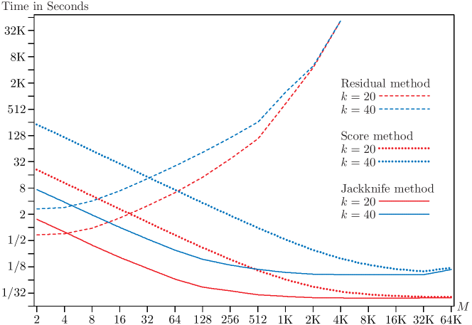
Figure 1: Timings for three ways to compute CV₃

Notes: The sample size is $N=1,048,576=1024K$, where $K=1024=2^{10}$. The number of clusters varies from 16 to $512K$. All clusters have $M=N/G$ observations, so that cluster sizes vary from 2 to $64K$. The number of regressors $k$ is either 20 or 40. Times required to compute $\hat{\bm{\beta}}$ are included; see text. All computations were performed in Fortran using one core of an Intel i9-13900K processor.

Figure 1 shows the time in seconds, on a log₂ scale, for each of the three methods and the two datasets as a function of cluster sizes $M=N/G$, which vary from 2 to $64K$. These times include the time required to compute the OLS estimates. For both the jackknife and score methods, there is considerable overlap between the computations needed for the OLS estimates and the ones needed for CV₃. Thus, for large clusters, the cost of computing the OLS estimates and CV₃ together using one or both of these methods was sometimes less than the cost of computing the OLS estimates alone. This is probably because of cache congestion, which seems to be alleviated by forming ${\bm{X}}^{\top}{\bm{X}}$ on a cluster-by-cluster basis. For large clusters, the speed of all methods could almost certainly be increased by using a fast BLAS implementation. However, in the interest of programming ease, we have not done this. The jackknife and score methods are already very fast.

In Figure 1, the residual method works well for very small values of $M$. It is always the fastest method for $M\leq 4$. We did not perform any timings for $M=1$, where CV₃ reduces to HC₃, because we would have needed a different program that eliminated the loops within each cluster to obtain optimal results. But the residual method is certainly the fastest one for this case. However, its cost rises very rapidly as $M$ increases. Results for this method are only shown for $M\leq 4096$, because using it for larger values would have been prohibitively costly. For the largest values of $M$, the cost of the residual method is almost the same for $k=20$ and $k=40$, because it is dominated by the computations needed to form and invert the ${\bm{M}}_{gg}$ matrices.

In contrast, both the score and jackknife methods become faster as $M$ increases and $G$ consequently decreases, except that, when $k=40$, they are both a bit slower for $M=64K$ than for $M=32K$. This probably occurs because of cache congestion. The jackknife method is always quicker than the score method. For small values of $M$, it seems to be faster by a factor of about 12 when $k=20$ and by a factor of about 26 when $k=40$. However, the advantage of the jackknife method gradually diminishes as $M$ increases. When $M=64K$, so that there are only 16 clusters, the jackknife method is only slightly faster.

It is easy to see that the jackknife method will have a big advantage over the residual method whenever cluster sizes vary much, even if most of them are very small. Imagine a sample with, say, 1000 equal-sized clusters and $M=5$. For such a sample, the residual and jackknife methods will perform about the same. Suppose we then merge 100 of the tiny clusters into one large cluster with 500 observations. Doing this will reduce the cost of the jackknife method slightly, but it will greatly increase the cost of the residual method. Indeed, when there is even a single very large cluster, the latter inevitably becomes extremely slow.

Based on these results, the jackknife method for computing CV₃ is clearly the procedure of choice unless all clusters are tiny (say, $N_{g}\leq 5$ for all $g$). For datasets with large clusters, an efficient implementation of this method (such as the one provided by the summclust package mentioned in Section 3), can compute both the OLS estimates and the CV₃ variance matrix in roughly the same amount of time as a reasonably fast program for the OLS estimates alone.

5 New Versions of the Wild Cluster Bootstrap

The existing WCR bootstrap is based on CV₁ standard errors and the restricted empirical score vectors defined in 25 below. Henceforth, we will refer to this as the classic WCR bootstrap, or WCR-C. It often works well, but not always. We therefore propose three new versions of the WCR bootstrap, along with three corresponding versions of the WCU bootstrap. These are based on two distinct modifications. One involves replacing CV₁ by CV₃. The other involves modifying the scores used in the bootstrap DGP, in the hope that the modified bootstrap DGP will provide a better approximation to the unknown process that actually generated the data.

We first discuss the bootstrap DGPs for all versions of the wild cluster bootstrap, expressing them in terms of scores instead of observations. This approach is intuitive and computationally attractive (Roodman et al., 2019; MacKinnon, 2022). In terms of the $G$ score vectors, a generic wild cluster bootstrap DGP is

$${\bm{s}}_{g}^{*b}=v_{g}^{*b}\ddot{\bm{s}}_{g},\quad g=1,\ldots,G,\quad b=1,\ldots,B,$$ (24)

where $b$ indexes bootstrap samples, $v_{g}^{*b}$ is a random variate with mean 0 and variance 1, and the $\ddot{\bm{s}}_{g}$ are empirical score vectors to be discussed below. In most cases, it seems to be best to generate the $v_{g}^{*b}$ using the Rademacher distribution, which takes the values 1 and $-1$ with equal probabilities (Davidson and Flachaire, 2008; Djogbenou et al., 2019). However, since the number of possible Rademacher bootstrap samples that are distinct from the original sample is only $2^{G}-1$, it is better to use a distribution with more mass points, such as the six-point distribution proposed in Webb (2022), when $G$ is less than about 12.

The vector $\ddot{\bm{s}}_{g}$ in 24 is an empirical score vector for the $g^{\kern 0.5833pt{\rm th}}$ cluster. For the WCU-C bootstrap, it is simply the unrestricted empirical score vector $\hat{\bm{s}}_{g}={\bm{X}}_{g}^{\top}\hat{\bm{u}}_{g}$. For the WCR-C bootstrap, it is the restricted empirical score vector $\tilde{\bm{s}}_{g}$ defined as

$$\tilde{\bm{s}}_{g}={\bm{X}}_{g}^{\top}{\bm{y}}_{g}-{\bm{X}}_{g}^{\top}{\bm{X}}_{g}\tilde{\bm{\beta}},\quad g=1,\ldots,G,$$ (25)

where $\tilde{\bm{\beta}}$ is the vector of OLS estimates under the null hypothesis. Like $\hat{\bm{\beta}}$, $\tilde{\bm{s}}_{g}$ is a $k$-vector, even though some elements of $\tilde{\bm{\beta}}$ may equal zero or satisfy other linear restrictions. The bootstrap DGP 24 looks very much like the one for the wild score cluster bootstrap for nonlinear models proposed in Kline and Santos (2012). In the context of 1, however, it is just a different way of writing the bootstrap DGP for the wild cluster bootstrap.

In order to calculate a bootstrap $P$ value or a bootstrap confidence interval, we need to compute $B$ bootstrap test statistics indexed by $b$. These depend only on the bootstrap scores in 24 and the matrix $({\bm{X}}^{\top}{\bm{X}})^{-1}$. For each bootstrap sample, we use ${\bm{s}}_{g}^{*b}$ to obtain a bootstrap estimate, not of ${\bm{\beta}}$ itself, but of the vector ${\bm{\delta}}={\bm{\beta}}-\ddot{\bm{\beta}}$, where $\ddot{\bm{\beta}}=\tilde{\bm{\beta}}$ for the WCR bootstrap and $\ddot{\bm{\beta}}=\hat{\bm{\beta}}$ for the WCU bootstrap. This estimate is simply

$$\hat{\bm{\delta}}^{*b}=({\bm{X}}^{\top}{\bm{X}})^{-1}\sum_{g=1}^{G}{\bm{s}}_{g}^{*b}=({\bm{X}}^{\top}{\bm{X}})^{-1}{\bm{s}}^{*b},$$ (26)

where ${\bm{s}}^{*b}=\sum_{g=1}^{G}{\bm{s}}_{g}^{*b}$. When $v_{g}^{*b}=1$ for all $g$, the bootstrap sample is the same as the original sample. In this very special case, $\hat{\bm{\delta}}^{*b}={\bm{0}}$ for the WCU bootstrap, and $\hat{\bm{\delta}}^{*b}=\hat{\bm{\beta}}-\tilde{\bm{\beta}}$ for the WCR bootstrap.

If we are testing the hypothesis that $\beta_{j}=0$, where $\beta_{j}$ is an element of ${\bm{\beta}}$, then we just need to multiply the $j^{\kern 0.5833pt{\rm th}}$ row of $({\bm{X}}^{\top}{\bm{X}})^{-1}$ by ${\bm{s}}^{*b}$ in order to obtain $\hat{\delta}_{j}^{*b}$, the $j^{\kern 0.5833pt{\rm th}}$ element of ${\bm{\delta}}^{*b}$. The bootstrap $t$-statistic is then equal to

$$t_{j}^{*b}=\frac{\hat{\delta}_{j}^{*b}}{{\rm se}(\hat{\delta}_{j}^{*b})}\kern 0.83328pt,$$ (27)

where ${\rm se}(\cdot)$ denotes the standard error formula used to obtain $t_{j}$, the original $t$-statistic. We automatically get the correct numerator, which is $\hat{\beta}_{j}^{*b}$ for the WCR bootstrap, since $\ddot{\bm{\beta}}=\tilde{\bm{\beta}}$, and $\hat{\beta}_{j}^{*b}-\hat{\beta}_{j}$ for the WCU bootstrap, since $\ddot{\bm{\beta}}=\hat{\bm{\beta}}$. As usual, a symmetric bootstrap $P$ value is then given by

$$P_{\rm S}^{*}(t_{j})=\frac{1}{B}\sum{\mathbb{I}}\big{(}|t_{j}^{*b}|>|t_{j}|\big{)},$$ (28)

where ${\mathbb{I}}(\cdot)$ denotes the indicator function. The bootstrap $P$ value in 28 is simply the fraction of the bootstrap samples for which $|t_{j}^{*b}|$ is more extreme than $|t_{j}|$. The value of $B$ should be chosen so that $\alpha(B+1)$ is an integer, where $\alpha$ is the level of the test (Racine and MacKinnon, 2007). It is common to use $B=999$, but $B=9,\kern-0.83328pt999$ and (when feasible) $B=99,\kern-0.83328pt999$ are better choices.

In the classic versions of the wild cluster bootstrap, the standard error formula in 27 is ${\rm se}_{1}(\cdot)$, the square root of the $j^{\kern 0.5833pt{\rm th}}$ diagonal element of CV₁. But the results in Section 3 make it equally feasible to use standard errors based on CV₃, even in large samples. This gives us new versions of both the WCR and WCU bootstraps, which we will refer to as WCR-V and WCU-V, because only the variance matrices have changed. The bootstrap standard errors can be calculated without computing an entire variance matrix for each bootstrap sample. For example, the CV₃ standard error of $\hat{\delta}_{j}^{*b}$ is just

$${\rm se}_{3}(\hat{\delta}_{j}^{*b})=\left(\frac{G-1}{G}\sum_{g=1}^{G}\big{(}\hat{\delta}_{j(g)}^{*b}-\hat{\delta}_{j}^{*b}\big{)}^{2}\right)^{\!\!1/2}\kern-0.83328pt,$$ (29)

where $\hat{\delta}_{j(g)}^{*b}$ is the $j^{\kern 0.5833pt{\rm th}}$ element of the vector

$$\hat{\bm{\delta}}_{(g)}^{*b}=({\bm{X}}^{\top}\!{\bm{X}}-{\bm{X}}_{g}^{\top}\!{\bm{X}}_{g})^{-1}({\bm{s}}^{*b}-{\bm{s}}_{g}^{*b}).$$ (30)

Only $\hat{\delta}_{j}^{*b}$ and the $\hat{\delta}_{j(g)}^{*b}$ need to be computed for each bootstrap sample. In 26 and 30, the first terms are invariant across bootstrap samples and only need to be computed once.

We now have two versions of the WCR bootstrap, WCR-C and WCR-V, and two versions of the WCU bootstrap, WCU-C and WCR-V. The two WCR bootstraps use the bootstrap DGP 24 with $\ddot{\bm{s}}_{g}=\tilde{\bm{s}}_{g}$, and the two WCU bootstraps use the bootstrap DGP 24 with $\ddot{\bm{s}}_{g}=\hat{\bm{s}}_{g}$. The “C” and “V” versions calculate both the actual and bootstrap test statistics using ${\rm se}_{1}(\cdot)$ and ${\rm se}_{3}(\cdot)$, respectively. These bootstrap methods use the restricted or unrestricted empirical scores in their raw form. But empirical scores differ from true scores, because residuals differ from disturbances. It therefore seems attractive to replace the empirical score vectors by modified score vectors that implicitly rescale the residuals on a cluster-by-cluster basis. This is analogous to methods discussed in Davidson and Flachaire (2008) and MacKinnon (2013) for the ordinary wild bootstrap. However, quite a lot more algebra is needed.

For the WCU bootstrap, we can simply replace the vectors $\ddot{\bm{s}}_{g}$ in 24 with the modified empirical score vectors $\acute{\bm{s}}_{g}$ defined in 11. Using 11 is expensive for large clusters, but the result 19 lets us compute $\acute{\bm{s}}_{g}$ very rapidly as

$$\acute{\bm{s}}_{g}={\bm{X}}^{\top}{\bm{X}}\big{(}\hat{\bm{\beta}}-\hat{\bm{\beta}}^{(g)}\big{)},\quad g=1,\ldots,G.$$ (31)

For large clusters, using 14 to compute the $\acute{\bm{s}}_{g}$ is much faster than using 11, but using 31 is faster still; see Section 4. This yields two new bootstrap methods, which we will refer to as WCU-S and WCU-B, respectively. The WCU-S bootstrap (S for score) employs the modified score vectors $\acute{\bm{s}}_{g}$ instead of $\hat{\bm{s}}_{g}$, but it uses the familiar ${\rm se}_{1}(\cdot)$ standard error. The WCU-B bootstrap (B for both) employs both the modified score vectors and the ${\rm se}_{3}(\cdot)$ standard error.

Finding the analogous versions of the WCR bootstrap takes a bit more work. We need to specify a restricted wild bootstrap DGP based on modified score vectors. Suppose the restrictions have the usual linear form, ${\bm{R}}{\bm{\beta}}={\bm{r}}$, for a given matrix ${\bm{R}}$ and a given vector ${\bm{r}}$. We can write this equivalently in terms of free parameters, $\bm{\phi}$, as ${\bm{\beta}}={\bm{H}}\bm{\phi}+{\bm{h}}$ for a given matrix ${\bm{H}}$ and a given vector ${\bm{h}}$. Then the modified score vectors are

$$\dot{\bm{s}}_{g}={\bm{X}}_{g}^{\top}\tilde{\bm{M}}_{gg}^{-1}({\bm{y}}_{g}-{\bm{X}}_{g}\tilde{\bm{\beta}}),$$ (32)

which are the analogs of the $\acute{\bm{s}}_{g}$ from 11. Here $\tilde{\bm{M}}_{gg}$ is the $g^{\kern 0.5833pt{\rm th}}$ diagonal block of the projection matrix $\tilde{\bm{M}}={\bf I}-\tilde{\bm{X}}(\tilde{\bm{X}}^{\top}\tilde{\bm{X}})^{-1}\tilde{\bm{X}}^{\top}$, where $\tilde{\bm{X}}={\bm{X}}{\bm{H}}$. However, evaluating 32 is computationally infeasible when the clusters are not all small. We need to replace 32 by something that is feasible for any sample size.

The first step is to compute $\tilde{\bm{\beta}}={\bm{H}}\tilde{\bm{\phi}}+{\bm{h}}$, where $\tilde{\bm{y}}={\bm{y}}-{\bm{X}}{\bm{h}}$ and $\tilde{\bm{\phi}}=(\tilde{\bm{X}}^{\top}\tilde{\bm{X}})^{-1}\tilde{\bm{X}}^{\top}\tilde{\bm{y}}$. The corresponding estimates when cluster $g$ is omitted are $\tilde{\bm{\beta}}^{(g)}={\bm{H}}\tilde{\bm{\phi}}^{(g)}+{\bm{h}}$, where

$$\tilde{\bm{\phi}}^{(g)}=(\tilde{\bm{X}}^{\top}\tilde{\bm{X}}-\tilde{\bm{X}}_{g}^{\top}\tilde{\bm{X}}_{g})^{-1}(\tilde{\bm{X}}^{\top}\tilde{\bm{y}}-\tilde{\bm{X}}_{g}^{\top}\tilde{\bm{y}}_{g}),\quad g=1,\ldots,G.$$ (33)

Then it can be shown that

$$\dot{\bm{s}}_{g}={\bm{X}}_{g}^{\top}\kern 0.41672pt\tilde{\bm{y}}_{g}-{\bm{X}}_{g}^{\top}\tilde{\bm{X}}_{g}\tilde{\bm{\phi}}^{(g)},\quad g=1,\ldots,G.$$ (34)

To see that 32 and 34 are equal, note that the right-hand side of 34 is

$${\bm{X}}_{g}^{\top}\big{(}\tilde{\bm{y}}_{g}-\tilde{\bm{X}}_{g}(\tilde{\bm{X}}^{\top}\tilde{\bm{X}}-\tilde{\bm{X}}_{g}^{\top}\tilde{\bm{X}}_{g})^{-1}(\tilde{\bm{X}}^{\top}\tilde{\bm{y}}-\tilde{\bm{X}}_{g}^{\top}\tilde{\bm{y}}_{g})\big{)}$$

$$\quad={\bm{X}}_{g}^{\top}\big{(}\tilde{\bm{y}}_{g}-\tilde{\bm{X}}_{g}\big{(}(\tilde{\bm{X}}^{\top}\tilde{\bm{X}})^{-1}+(\tilde{\bm{X}}^{\top}\tilde{\bm{X}})^{-1}\tilde{\bm{X}}_{g}^{\top}\tilde{\bm{M}}_{gg}^{-1}\tilde{\bm{X}}_{g}(\tilde{\bm{X}}^{\top}\tilde{\bm{X}})^{-1}\big{)}(\tilde{\bm{X}}^{\top}\tilde{\bm{y}}-\tilde{\bm{X}}_{g}^{\top}\tilde{\bm{y}}_{g})\big{)},$$

where the equality uses the updating formula 21 applied to $\tilde{\bm{X}}$, $\tilde{\bm{X}}_{g}$, and $\tilde{\bm{M}}_{gg}^{-1}$. Then we use the fact that $\tilde{\bm{\phi}}=(\tilde{\bm{X}}^{\top}\tilde{\bm{X}})^{-1}\tilde{\bm{X}}^{\top}\tilde{\bm{y}}$ together with the relation $\tilde{\bm{X}}_{g}(\tilde{\bm{X}}^{\top}\tilde{\bm{X}})^{-1}\tilde{\bm{X}}_{g}^{\top}=\tilde{\bm{P}}_{gg}={\bf I}-\tilde{\bm{M}}_{gg}$ to rewrite the last expression as

$${\bm{X}}_{g}^{\top}\big{(}\tilde{\bm{y}}_{g}-\tilde{\bm{X}}_{g}\tilde{\bm{\phi}}-({\bf I}-\tilde{\bm{M}}_{gg})\tilde{\bm{M}}_{gg}^{-1}\tilde{\bm{X}}_{g}\tilde{\bm{\phi}}+({\bf I}-\tilde{\bm{M}}_{gg})\tilde{\bm{y}}_{g}+({\bf I}-\tilde{\bm{M}}_{gg})\tilde{\bm{M}}_{gg}^{-1}({\bf I}-\tilde{\bm{M}}_{gg})\tilde{\bm{y}}_{g}\big{)}$$ (35)

$$\quad={\bm{X}}_{g}^{\top}\tilde{\bm{M}}_{gg}^{-1}(\tilde{\bm{y}}_{g}-\tilde{\bm{X}}_{g}\tilde{\bm{\phi}}).$$

Replacing $\tilde{\bm{y}}_{g}$ by ${\bm{y}}_{g}-{\bm{X}}_{g}{\bm{h}}$ and $\tilde{\bm{X}}_{g}$ by ${\bm{X}}_{g}{\bm{H}}$, and using the fact that ${\bm{H}}\tilde{\bm{\phi}}=\tilde{\bm{\beta}}-{\bm{h}}$, the right-hand side of 35 equals 32.

An important special case is the restriction that $\beta_{k}=0$. This is obtained by setting ${\bm{R}}=(0,\ldots,0,1)$ and ${\bm{r}}=0$, or, equivalently, ${\bm{H}}=({\bf I}_{k-1},{\bm{0}})^{\top}$ and ${\bm{h}}={\bm{0}}$. In this case, we find that $\tilde{\bm{X}}={\bm{X}}_{1}$, which contains the first $k-1$ columns of ${\bm{X}}$, and $\tilde{\bm{\phi}}=\tilde{\bm{\beta}}_{1}=({\bm{X}}_{1}^{\top}{\bm{X}}_{1})^{-1}{\bm{X}}_{1}^{\top}{\bm{y}}$. The corresponding estimates when each cluster is omitted in turn are

$$\tilde{\bm{\beta}}_{1}^{(g)}=({\bm{X}}_{1}^{\top}\!{\bm{X}}_{1}-{\bm{X}}_{1g}^{\top}\kern 0.83328pt{\bm{X}}_{1g})^{-1}({\bm{X}}_{1}^{\top}{\bm{y}}-{\bm{X}}_{1g}^{\top}\kern 0.83328pt{\bm{y}}_{g}),\quad g=1,\ldots,G,$$ (36)

where ${\bm{X}}_{1g}$ contains the first $k-1$ columns of ${\bm{X}}_{g}$. Then 34 reduces to

$$\dot{\bm{s}}_{g}={\bm{X}}_{g}^{\top}\kern 0.41672pt{\bm{y}}_{g}-{\bm{X}}_{g}^{\top}\kern 0.83328pt{\bm{X}}_{1g}\kern 0.41672pt\tilde{\bm{\beta}}_{1}^{(g)},\quad g=1,\ldots,G.$$ (37)

Exactly the same arguments that led to 34 can be applied to the modified unrestricted empirical scores, giving us

$$\acute{\bm{s}}_{g}={\bm{X}}_{g}^{\top}\kern 0.41672pt{\bm{y}}_{g}-{\bm{X}}_{g}^{\top}{\bm{X}}_{g}\hat{\bm{\beta}}^{(g)},\quad g=1,\ldots,G.$$ (38)

Either 31 or 38 can be used to compute the $\acute{\bm{s}}_{g}$, and both are computationally attractive. However, in situations where both $\dot{\bm{s}}_{g}$ and $\acute{\bm{s}}_{g}$ need to be computed, 38 may offer some programming advantages relative to 31 due to its similarity to 34.

The scalar factors in 6 and 10 do not appear in the bootstrap DGPs that correspond to them, because rescaling all the bootstrap scores by the same factor has no impact on the bootstrap $t$-statistics. From 26 and 30, multiplying all the ${\bm{s}}_{g}^{*b}$ by a scalar $C$ simply makes $\hat{\bm{\delta}}^{*b}$ and all the $\hat{\bm{\delta}}_{(g)}^{*b}$ larger by a factor of $C$. This also makes the empirical scores for every bootstrap sample larger by the same factor. Therefore, from 6, 8, and 10, the variance matrices become larger by a factor of $C^{\kern 0.2917pt2}$ and the standard errors by a factor of $C$. The factors of $C$ in the numerator and denominator of $t_{j}^{*b}$ cancel out, leaving the bootstrap $t$-statistics unchanged.

However, no cancellation occurs for bootstrap tests of $\beta_{j}=0$ based directly on $\hat{\beta}_{j}$ and its bootstrap analog of $\hat{\delta}_{j}^{*b}$. In this case, multiplying the right-hand side of 24 by the square root of $G(N-1)/((G-1)(N-k))$ for methods that use CV₁ and by the square root of $(G-1)/G$ for methods that use CV₃ should improve the correspondence between the bootstrap DGP and the unknown true DGP. The usual theory of higher-order refinements for the bootstrap suggests that it is generally better to studentize (Hall, 1992). However, there may be cases in which unstudentized test statistics are of interest (Canay, Santos and Shaikh, 2021). But since we have eight studentized bootstrap methods to study, we do not consider unstudentized ones further.

To generate the transformed scores needed for the WCR/WCU-S and WCR/WCU-B bootstraps, 31 and 38 must be used for all $G$ clusters. In the event that $\hat{\bm{\beta}}^{(h)}$ and $\tilde{\bm{\beta}}^{(h)}$ cannot be calculated for cluster $h$, we have two choices. The simplest is to replace the inverses in 15 and 36 by generalized inverses. Alternatively, we could use $\hat{\bm{s}}_{h}$ instead of $\acute{\bm{s}}_{h}$ and $\tilde{\bm{s}}_{h}$ instead of $\dot{\bm{s}}_{h}$, along with the transformed scores for the remaining clusters. The latter would be appropriate if we have chosen to omit the problematic clusters when computing the cluster-jackknife variance matrix; see the discussion at the end of Section 3.

Table 1: Eight versions of the wild cluster bootstrap

	Standard errors based on
Scores in bootstrap DGP 24	CV1	CV3
Null hypothesis imposed
$\tilde{\bm{s}}_{g}$ defined in 25	WCR-C	WCR-V
$\dot{\bm{s}}_{g}$ defined in 37	WCR-S	WCR-B
Null hypothesis not imposed
$\hat{\bm{s}}_{g}={\bm{X}}_{g}^{\top}\hat{\bm{u}}_{g}$	WCU-C	WCU-V
$\acute{\bm{s}}_{g}$ defined in 31 or 38	WCU-S	WCU-B

Notes: WCR-C and WCU-C are the classic versions of the wild cluster restricted and wild cluster unrestricted bootstraps. WCR-S and WCU-S employ transformed scores with the usual CV₁ variance matrix. WCR-V and WCU-V employ the usual scores with the CV₃ variance matrix. WCR-B and WCU-B employ both transformed scores and CV₃.

Table 1 provides a convenient summary of the eight wild cluster bootstrap methods that we have discussed. Conceptually, they differ along two dimensions. The horizontal dimension represents the way in which the standard errors for both the actual and bootstrap test statistics are calculated. The vertical dimension represents the score vectors used in the four versions of the bootstrap DGP 24. Note that the boottest and fwildclusterboot packages now provide fast implementations of the WCR/WCU-S bootstraps as well as the classic ones. This is possible because, in contrast to the WCR/WCU-V and WCR/WCU-B bootstraps, the former do not involve any jackknife calculations for the bootstrap samples. Once the transformed scores have been computed, the fast bootstrap algorithm proposed in Roodman et al. (2019) applies directly to the WCR/WCU-S bootstraps.

It seems highly likely that all the methods discussed in this section are asymptotically valid, in the sense that, under suitable regularity conditions, the rejection frequencies for any test converge to the nominal level of the test as $G\to\infty$. Formal proofs could be obtained by modifying the arguments in Djogbenou et al. (2019). For the WCU bootstrap methods, the key fact is that the modified empirical score vectors $\acute{\bm{s}}_{g}$ computed using 31 or 38 are asymptotically equal to the ordinary empirical score vectors $\hat{\bm{s}}_{g}$. For the WCR bootstrap methods, the key fact is that the modified restricted empirical score vectors $\dot{\bm{s}}_{g}$ defined in 34 are asymptotically equal to the ordinary restricted empirical score vectors $\tilde{\bm{s}}_{g}$ in 25.

6 Monte Carlo Simulations

Simulation results in MacKinnon and Webb (2017, 2018), Brewer et al. (2018), Djogbenou et al. (2019), MacKinnon (2022), and several other papers have shown that the reliability of bootstrap and asymptotic methods for cluster-robust inference depends heavily on the number of clusters, the extent to which cluster sizes vary, and (in the case of treatment effects) both the number of treated clusters and their sizes. Many of our experiments therefore focus on these features.

The model we consider is

$$y_{gi}=\beta_{1}+\sum_{j=2}^{k}\beta_{j}X_{jgi}+u_{gi},\quad g=1,\ldots,G,\quad i=1,\ldots,N_{g},$$ (39)

where the $u_{gi}$ are generated by a normal random-effects model with intra-cluster correlation $\rho$. The way in which the $k-1$ non-constant regressors are generated varies across the experiments. The hypothesis to be tested is that $\beta_{k}=0$.

In most of our experiments, there are $N=400G$ observations, which are divided among the $G$ clusters using the formula

$$N_{g}=\left[N\frac{\exp(\gamma g/G)}{\sum_{j=1}^{G}\exp(\gamma j/G)}\right]\!,\quad g=1,\ldots,G-1,$$ (40)

where $[x]$ means the integer part of $x$. The value of $N_{G}$ is then set to $N-\sum_{g=1}^{G-1}N_{g}$. The key parameter here is $\gamma$, which determines how uneven the cluster sizes are. When $\gamma=0$ and $N/G$ is an integer, 40 implies that $N_{g}=N/G$ for all $g$. For $\gamma>0$, cluster sizes vary more and more as $\gamma$ increases. The largest value of $\gamma$ that we use is 4. In that case, when $G=24$ and $N=9600$, the largest cluster (1513 observations) is about 47 times as large as the smallest cluster (32 observations). In contrast, when $\gamma=2$, the largest cluster (899 observations) is just under seven times as large as the smallest (130 observations).

The sample sizes that we employ are unusually large for experiments of this type. Since cluster-robust inference is often used with samples that have hundreds of thousands or even millions of observations, we want our results to apply to such cases. In preliminary experiments, we found that the results tended to change slightly, but systematically, as small values of $N/G$ were increased. Results for $N/G>400$ are very similar to ones for $N/G=400$, so we use 400 in all the experiments based on 40. Because the bootstrap samples are generated using scores, the cost of the experiments increases much less than proportionally with $N/G$.

All experiments use $400,\kern-0.83328pt000$ replications. This number is so large that experimental randomness is negligible. The most important determinant of computational cost is $k$, the number of regressors. As can be seen from 24 and 34 or 38, generating each bootstrap sample involves $O(k^{2}G)$ operations. So does calculating the test statistics using either CV₁ or CV₃. Thus the experiments can be somewhat costly when $k$ is large. Nevertheless, many of our experiments involve $k\geq 10$. We do this because results in MacKinnon (2022) suggest that the performance of many methods of inference deteriorates as $k$ increases. Previous Monte Carlo experiments, which often use $k\leq 3$, may therefore have tended to give too optimistic a picture.

It might seem that substantial savings could be achieved by partialing out all regressors except the one(s) of interest prior to performing the bootstrap. However, this trick only works in certain special cases. For methods based on the jackknife, it is easy to see the problem. If we were to partial out some of the regressors prior to computing the delete-one-cluster estimates in 15, then the computed $\hat{\bm{\beta}}^{(g)}$ would depend on the values of the partialed-out regressors for the full sample, including those in the $g^{\kern 0.5833pt{\rm th}}$ cluster which was supposed to be deleted. Consequently, the values of the delete-one-cluster estimates would be incorrect if we partialed out any regressor that affects more than one cluster (such as industry-level fixed effects with firm-level clustering).

An important exception is when the regressors that are partialed out are cluster fixed effects or fixed effects at a finer level (such as firm-level fixed effects with industry-level clustering), because each of them affects only some or all of the observations within a single cluster. In fact, it is essential to partial out fixed effects of this type if using a generalized inverse is to be avoided.

6.1 Test Size

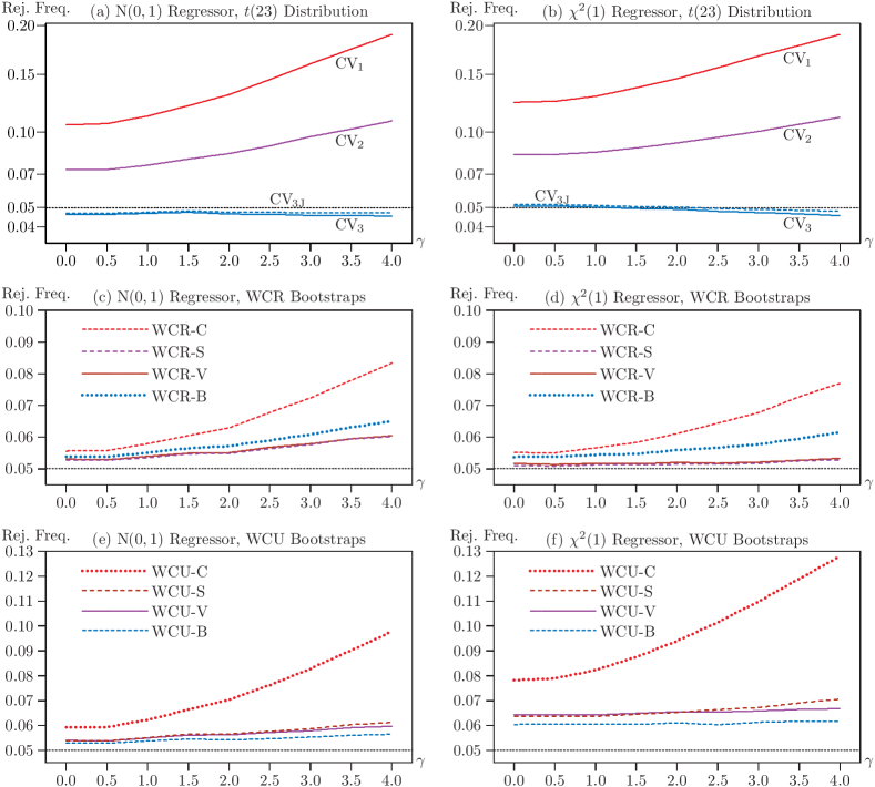
Figure 2: Rejection frequencies as a function of $\gamma$

Notes: The vertical axes show rejection frequencies for tests of $\beta_{k}=0$ in 39 at the .05 level. Results are based on $400,\kern-0.66663pt000$ replications, with $B=399$ bootstrap samples. There are 24 clusters, 9600 observations, and 10 regressors, with $\rho=0.10$. The extent to which cluster sizes vary increases with $\gamma$; see 40.

The experiments in this subsection deal with rejection frequencies under the null hypothesis. We consider both asymptotic tests based on the $t(G-1)$ distribution and the wild cluster bootstrap tests listed in Table 1.

The experiments in Figure 2 focus on variation in cluster sizes. There are always 9600 observations, 24 clusters, and 10 regressors. Cluster sizes vary according to 40. Regressors 2 through $k-1$ in 39 follow a normal random-effects model that yields intra-cluster correlations of 0.50. The test regressor either follows the same normal distribution as the others (in the three panels on the left), or a $\chi^{2}(1)$ distribution (in the three panels on the right). In the latter case, it is the square of a normally distributed random variable generated by the same random-effects model as the other regressors. The disturbances are also generated by such a model, but with $\rho=0.10$. We focus on rejection frequencies for a test that $\beta_{k}=0$ at the 5% level.

The results for asymptotic tests, based on the $t(23)$ distribution and shown in Panels (a) and (b), are striking. Note that a square-root transformation has been applied to the vertical axis to prevent these panels from being too tall. Tests based on CV₁ over-reject substantially. The extent of the over-rejection increases with $\gamma$, and, except for $\gamma=4$, it is more severe in Panel (b) than in Panel (a). A regressor that follows the $\chi^{2}(1)$ distribution necessarily has some extreme values. These become points of high leverage, which makes inference more difficult in Panel (b).

Although tests based on CV₂ always reject considerably less often than ones based on CV₁, they also over-reject significantly and to an extent that increases with $\gamma$. In contrast, tests based on CV₃ and CV_3J either under-reject slightly all the time, in Panel (a), or under-reject very slightly for larger values of $\gamma$, in Panel (b). The results for CV₃ and CV_3J are extremely similar. The latter always rejects more often than the former, because the difference between 17 and 18 is the positive semi-definite matrix $((G-1)/G)(\hat{\bm{\beta}}-\bar{\bm{\beta}})(\hat{\bm{\beta}}-\bar{\bm{\beta}})^{\top}$. Since CV₃ tends to under-reject slightly in Figure 2, it might seem that CV_3J is to be preferred. However, as we shall see, there are also many cases in which CV₃ over-rejects, and CV_3J therefore over-rejects slightly more. In practice, it would be perfectly reasonable to report either CV₃ or CV_3J. We never encountered a case in which it made any real difference.

The results for the WCR bootstrap tests, shown in Panels (c) and (d), are surprising. In the past, WCR-C has been the only variant of the WCR bootstrap, and numerous Monte Carlo experiments have suggested that it is the procedure of choice. But WCR-B performs notably better than WCR-C for every value of $\gamma$, and both WCR-V and WCR-S perform better still. Note that, although these two procedures perform almost the same here, this is not true in general. Oddly, all the WCR procedures perform better in Panel (d), where the test regressor is highly skewed, than they do in Panel (c), where it is Gaussian. The rather mediocre performance of WCR-C must be due, at least in part, to the fact that $k=10$, which is a larger number than has been used in most previous experiments; see Figure 3 below.

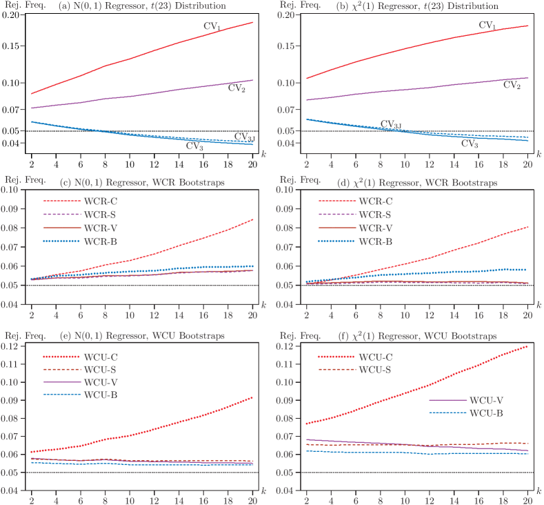
Figure 3: Rejection frequencies as a function of $k$

Notes: The vertical axes show rejection frequencies for tests of $\beta_{k}=0$ in 39 at the .05 level. Results are based on $400,\kern-0.66663pt000$ replications, with $\gamma=2$, $\rho=0.10$, and $B=399$ bootstrap samples. There are 24 clusters, 9600 observations, and $k$ regressors, where $k$ varies from 2 to 20 by 2.

Some of the results for the WCU bootstrap tests, shown in Panels (e) and (f), are also surprising. It is not a surprise that WCU-C rejects more often than WCR-C or that its performance is much worse in Panel (f) than in Panel (e). However, the fact that the other three WCU procedures over-reject much less often than WCU-C may well be surprising. In both panels, WCU-B is clearly the procedure of choice. WCU-V and WCU-S perform much better than WCU-C, but worse than WCU-B. In Panels (c) and (d), the differences between WCU-V and WCU-S are small, but larger than the differences between WCR-V and WCR-S.

Figure 3 is similar to Figure 2, but the number of regressors $k$ is now on the horizontal axis, and $\gamma=2$. In Panels (a) and (b), CV₁ over-rejects to an increasing extent as $k$ increases. So does CV₂, although it always over-rejects considerably less than CV₁. In contrast, CV₃ and CV_3J over-reject modestly for small values of $k$ and under-reject modestly for large ones.

Panels (c) and (d) look a lot like the same panels in Figure 2, even though what is on the horizontal axis is different. WCR-C performs quite well for very small values of $k$, but it over-rejects more and more severely as $k$ increases. WCR-B performs much better than WCR-C, but WCR-V and WCR-S perform even better. In Panel (d), where the test regressor is highly skewed, they both perform extremely well for all values of $k$.

Panels (e) and (f) also look a lot like the same panels in Figure 2. WCU-C performs quite poorly, over-rejecting more and more severely as $k$ increases. In contrast, WCU-B performs quite well in Panel (e) and fairly well in Panel (f), and there is no tendency for its performance to deteriorate as $k$ increases. As before, the two other bootstrap methods generally perform much better than WCU-C but slightly worse than WCU-B.

In the next set of experiments, we focus on what happens as $G$ increases. Figure 4 shows rejection frequencies as functions of $G$, which varies from 12 to 84 by 6, and implicitly also $N$, since $N=400G$. In these experiments, $\gamma=2$ and $k=10$. We report results for only five methods, instead of twelve. We omit CV₁ and CV₂, because they never perform very well, and CV_3J because it is almost identical to CV₃. Among the restricted bootstrap methods, we report WCR-C, because it was until now the procedure of choice. We also report WCR-S and WCR-B, but we do not report WCR-V, because it yields results nearly identical to those of WCR-S and is harder to compute. Among the unrestricted bootstrap methods, we report only WCU-B, because it always seems to outperform the other WCU methods.

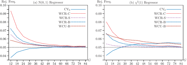
Figure 4: Rejection frequencies as a function of $G$

Notes: The vertical axes show rejection frequencies for tests of $\beta_{k}=0$ in 39 at the .05 level. Results are based on $400,\kern-0.66663pt000$ replications, with $\gamma=2$, $k=10$, $\rho=0.10$, and $B=399$ bootstrap samples. There are between 12 and 84 clusters, all multiples of 6, with 400 observations per cluster on average.

In Panel (a), using CV₃ with the $t(G-1)$ distribution under-rejects quite noticeably for very small values of $G$, but it performs extremely well for $G\geq 30$. The bootstrap methods always over-reject, with WCR-C always the worst of them. For $G\geq 42$, however, all the bootstrap methods perform very well, with WCR-S the winner by a tiny margin.

Panel (b) is more interesting than Panel (a). The extreme skewness of the $\chi^{2}(1)$ regressor apparently affects the results quite a bit, even when $G=84$. Using CV₃ with the $t(G-1)$ distribution under-rejects for small values of $G$ but over-rejects for larger values, where it is the worst method. Note that $G=24$, the value in Figures 2 and 3, is near where the curve for CV₃ crosses the .05 line in Figure 4. The best method is WCR-S in every case. It performs remarkably well for $G\geq 30$. However, all three WCR methods perform well for the larger values of $G$. Indeed, by most standards, every method shown in Panel (b) of Figure 4 works very well, unless $G$ is less than about 30. For $G=84$, CV₃ is the worst method, but even it rejects only 5.49% of the time. For comparison, CV₁ rejects 9.04% of the time, and CV₂ rejects 7.15%. The best method, WCR-S, rejects 4.97% of the time.

Many applications of cluster-robust inference involve treatment at the cluster level, and existing methods generally perform very poorly when either the number of treated clusters or the number of control clusters is small. Using CV₁ with the $t(G-1)$ distribution or WCU-C leads to severe over-rejection, and using WCR-C leads to severe under-rejection (MacKinnon and Webb, 2017, 2018). Our next set of experiments therefore focuses on the model

$$y_{gi}=\beta_{1}+{\bm{Z}}_{gi}{\bm{\beta}}_{2}+\beta_{k}x_{g}+u_{gi},$$ (41)

where $x_{g}$ is a treatment dummy, ${\bm{Z}}_{gi}$ is a row vector of other regressors, and $u_{gi}$ is generated by a random-effects model with intra-cluster correlation $\rho$. The treatment dummy equals 1 for $G_{1}$ of the $G$ clusters and 0 for the remaining $G_{0}=G-G_{1}$. The clusters that are treated are chosen at random. The ${\bm{Z}}_{gi}$ consist of eight more dummy variables. For each of these variables and each cluster, a probability $\pi_{g}$ between 0.25 and 0.75 is chosen at random for each replication. Then each observation for that variable in that cluster equals 1 with probability $\pi_{g}$ and 0 otherwise. Thus all the regressors are dummies, which vary at the individual level in a way that varies across clusters.

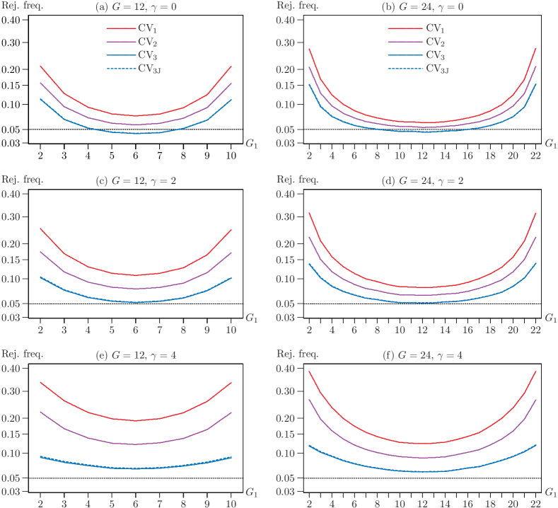
Figure 5: Rejection frequencies based on $t(G-1)$ distribution for treatment regression

Notes: The vertical axes, which have been subjected to a square-root transformation, show rejection frequencies for tests of $\beta_{k}=0$ in 41 at the .05 level. The horizontal axes show $G_{1}$, the number of treated clusters. Results are based on $400,\kern-0.66663pt000$ replications, with $k=10$ regressors and $\rho=0.10$. There are either 12 or 24 clusters, with 400 observations per cluster on average. Treated clusters are chosen at random.

Figure 5 shows rejection frequencies based on the $t(G-1)$ distribution. In the left-hand column, there are 12 clusters and 4800 observations. In the right-hand one, there are 24 clusters and 9600 observations. The value of $\gamma$ is 0 in the top row, 2 in the middle row, and 4 in the bottom row. The number of treated observations $G_{1}$ varies between 2 and $G-2$ on the horizontal axes. It would have been impossible to set $G_{1}=1$ or $G_{1}=G-1$, because CV₂, CV₃, and CV_3J cannot be computed in those cases. This is obvious from 15 for the jackknife-based estimators. When the single treated cluster is omitted, the coefficient of interest in $\hat{\bm{\beta}}^{(g)}$ is not identified.

As previous work has shown, tests that use CV₁ tend to over-reject severely when either $G_{0}$ or $G_{1}$ is small. This is evident in Figure 5. The over-rejection is worst in Panel (f), where both $\gamma$ and $G$ are largest. CV₂ over-rejects less than CV₁, but it still does not work very well, except perhaps for values of $G_{1}$ near $G/2$ when $\gamma=0$; see Panels (a) and (b). In contrast, CV₃ and CV_3J, which perform almost identically, are much less prone to over-reject than the other two CRVEs. They actually under-reject for values of $G_{1}$ fairly near $G/2$ when $\gamma=0$, and they perform very well for values of $G_{1}$ near $G/2$ when $\gamma=2$. Oddly, CV₃ and CV_3J over-reject less seriously for extreme values of $G_{1}$ when $\gamma$ is large than when $\gamma$ is small.

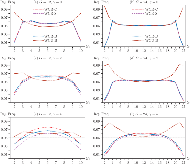
Figure 6: Bootstrap rejection frequencies for treatment regression

Notes: The vertical axes show rejection frequencies for tests of $\beta_{k}=0$ in 41 at the .05 level. The horizontal axes show $G_{1}$, the number of treated clusters. Results are based on $400,\kern-0.66663pt000$ replications, with $k=10$, $\rho=0.10$, and $B=399$ bootstrap samples. There are either 12 or 24 clusters, with 400 observations per cluster on average.

Figure 6 shows results for four bootstrap tests for the same set of experiments as in Figure 5. When $\gamma=0$, all three variants of the WCR bootstrap perform almost identically. However, as $\gamma$ increases, their performance starts to differ. WCR-S seems to reject least frequently, which is a good thing for intermediate values of $G_{1}$ and a bad thing for extreme values. In contrast, WCR-B under-rejects least severely for extreme values of $G_{1}$. However, for intermediate values, it over-rejects less than WCR-C but more than WCR-S.

The most surprising results in Figure 6 are the ones for the unrestricted wild bootstraps. We do not report results for WCU-C or WCU-S, because they would have required a much longer vertical axis. WCU-C rejects almost 28% of the time in its worst case ($G=24$, $G_{1}=2$, $\gamma=4$), and WCU-S rejects over 12% of the time in its worst case ($G=24$, $G_{1}=2$, $\gamma=0$). In contrast, WCU-B is arguably the best method overall when $G=12$, and it performs very well for intermediate values of $G_{1}$ when $G=24$. In addition, it never over-rejects as severely as CV₃ for extreme values of $G_{1}$.

Simulations in Djogbenou et al. (2019) suggest that many methods work poorly when one cluster is much bigger than the others. Even when $\gamma=4$, the largest cluster in our experiments is never dramatically larger than all the rest, although this happens quite often in empirical work. For instance, more than half of all incorporations in the United States occur in Delaware (Hu and Spamann, 2020). This implies that studies of the effects of corporate governance based on changes in state laws, where standard errors are clustered by state of incorporation, are likely to encounter severe errors of inference. To investigate this phenomenon, we create artificial samples with 50 clusters based on data for incorporations by year and state from Spamann and Wilkinson (2019). There are $205,\kern-0.83328pt566$ observations, of which $108,\kern-0.83328pt538$, or 52.80%, are for Delaware. The second-largest cluster is Nevada, with $17,\kern-0.83328pt010$ or 8.27%, and the smallest is Montana, with 101 or 0.05%.

We perform a set of experiments similar to the ones in Figures 5 and 6 using these artificial samples. There are 10 regressors, generated in the same way as before, with one exception. Because investigators are surely aware of whether or not the largest cluster (Delaware) is treated, it is always treated in our experiments. The other clusters to be treated (between 1 and 47 of them) are chosen at random. Because the largest cluster is always treated, the rejection frequencies are no longer the same for $G_{1}$ and $G-G_{1}$ treated clusters. However, since this is a pure treatment model, the results for $G_{1}$ treated clusters that include Delaware must be the same as the results for $G-G_{1}$ treated clusters that exclude Delaware.

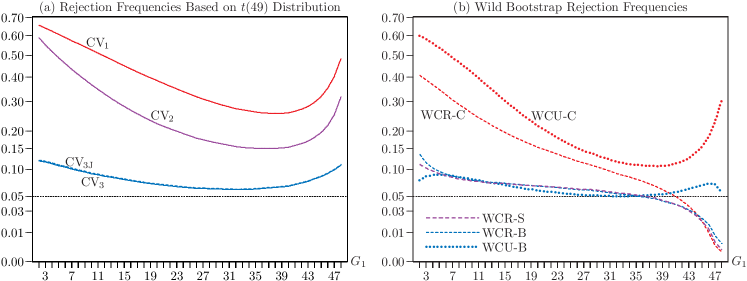
Figure 7: Rejection frequencies when a treated cluster is very large

Notes: The vertical axes show rejection frequencies for tests of $\beta_{k}=0$ in 41 at the .05 level. Results are based on $400,\kern-0.66663pt000$ replications, with $k=10$, $\rho=0.10$, and $B=399$. There are $205,\kern-0.66663pt566$ observations and 50 clusters, with cluster sizes proportional to incorporations in U.S. states. The largest cluster is always treated, and the other clusters are treated at random. The number of treated clusters varies from 2 to 14 by 1, from 16 to 36 by 2, and then from 38 to 48 by 1.

The results in Figure 7 are striking. In Panel (a), using either CV₁ or CV₂ leads to over-rejection that varies between severe and extreme. Using CV₃ and CV_3J also leads to over-rejection, but it is much less severe. For between 20 and 41 treated clusters, rejection frequencies are less than 0.07. In Panel (b), WCU-C over-rejects severely, and WCR-C can either over-reject or under-reject, often severely. In contrast, our new bootstrap methods work remarkably well. The best of them is WCU-B, which always rejects less than 9% of the time and sometimes rejects just about 5% of the time. WCR-S and WCR-B also perform much better than WCR-C, except when $G_{1}$ is very large, in which case they under-reject severely.

Even though it is based on real data, the distribution of cluster sizes in the experiments of Figure 7 is very extreme. The performance of CV₃ and three of our new bootstrap methods is far from perfect, but it is generally very much better than that of existing methods. Thus jackknife-based methods seem to be remarkably robust to heterogeneity in cluster sizes.

6.2 Test Power

It is natural to worry that a new test may be less powerful than existing tests, especially when it performs much better under the null hypothesis. In this section, we therefore investigate test power. Studying power is tricky, because it is unreasonable to compare tests that have noticeably different rejection frequencies under the null. If, for example, an asymptotic test rejects 15% of the time under the null and a bootstrap test rejects 6% of the time, then we would expect the asymptotic test to have substantially more power than the bootstrap test. But the additional power may be entirely spurious, simply reflecting the finite-sample over-rejection by the former.

One way to compare tests with different rejection frequencies under the null is to “size-adjust” them. But this approach has two serious conceptual difficulties. First, size-adjusted tests are infeasible. What do we learn by comparing tests that cannot actually be performed? Second, there are often many ways to size-adjust a given test, and they may yield quite different results. The idea of size-adjustment is to base rejection frequencies for tests under the alternative on critical values calculated by simulation under the null. But, in general, there exists an infinite number of DGPs that satisfy the null hypothesis. If they all yield the same critical values, then there is no problem. But if they yield different critical values, as will often be the case, then we have to choose which null DGP to use. It seems natural to make the null DGP used for critical values as close as possible to the alternative DGP. Davidson and MacKinnon (2006) suggests a particular way of doing this, based on the Kullback-Leibler information criterion, but this approach means using a different critical value for each set of values of the parameters under test.

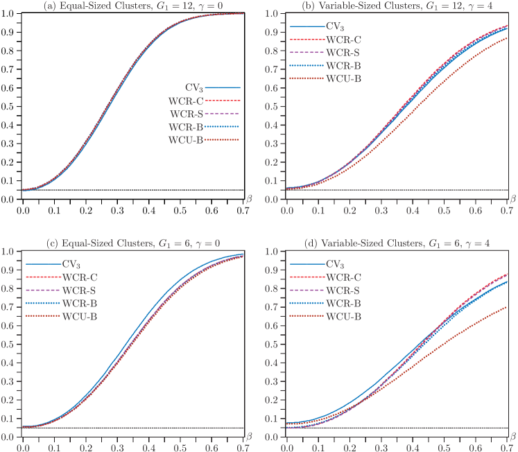
Figure 8: Power functions for several tests

Notes: The vertical axes show rejection frequencies for tests at the .05 level. Results are based on $400,\kern-0.66663pt000$ replications, with $G=24$, $N=9600$, $k=5$, $\rho=0.10$, and $B=999$. The hypothesis being tested is $\beta_{k}=0$ in 41. The horizontal axes show the values of $\beta$ in the DGP.

To avoid the difficulties just discussed, we focus on four cases where the tests of interest all perform quite well under the null. They are treatment experiments similar to the ones in Figures 5 and 6, with $G=24$, $N=9600$, and $k=5$. In Panels (a) and (b), $G_{1}=12$, so that precisely half the clusters are treated. In Panels (c) and (d), $G_{1}=6$, so that the effects of having few treated clusters are apparent but not severe. In order to avoid excessive power loss, we use $B=999$ for the bootstrap tests. We use $k=5$ instead of $k=10$ partly to reduce computational cost and partly to improve test performance under the null.

Figure 8 shows rejection frequencies as a function of $\beta_{k}$, the actual coefficient on the treatment dummy in 41, when the null hypothesis is that $\beta_{k}=0$. In Panels (a) and (c), $\gamma=0$, so that every cluster has exactly 400 observations. In Panel (a), the perfectly balanced case, all five power functions are visually indistinguishable. In Panel (c), where only six clusters are treated, CV₃ has noticeably more power than any of the bootstrap methods, which are all but identical.

In Panels (b) and (d), cluster sizes vary from 32 to 1513. All tests are now substantially less powerful than in Panels (a) and (c), because, whenever there is intra-cluster correlation, the information content of a sample declines as the cluster sizes become more variable. The most striking result in both panels is that WCU-B has noticeably less power than any of the other methods. This is especially true in Panel (d), where WCU-B over-rejects modestly under the null but becomes by far the least powerful method for larger values of $\beta_{k}$.

The pattern for CV₃ is similar but much less pronounced. Under the null hypothesis, it over-rejects slightly under the null in Panel (b) and noticeably in Panel (d), with rejection frequencies of 0.0612 and 0.0775, respectively. But for large enough values of $\beta_{k}$, it has less power than WCR-C and WCR-S, especially in Panel (d). The latter two methods also have slightly more power than WCR-B in Panel (b) and noticeably more in Panel (d) for large values of $\beta_{k}$. Interestingly, WCR-V, which for clarity is not shown in the figure, has somewhat less power than either WCR-C or WCR-S in Panels (b) and (d), where cluster sizes vary a lot. In contrast, it is almost indistinguishable from both these methods in Panels (a) and (c), where cluster sizes are constant.

Based on these results, the procedure of choice appears to be WCR-S. For larger values of $\beta_{k}$, it is always one of the two most powerful tests. WCR-C has similar power, and it also works well under the null in these experiments, but it is much more prone to over-reject than WCR-S in Figures 3, 4, 6 and 7. Happily, WCR-S is already available in computationally efficient packages for Stata, R, and Python; see Section 5.

6.3 Confidence Intervals

Cluster-robust standard errors and bootstrap methods are often used to form confidence intervals. Although we do not perform any Monte Carlo experiments explicitly to study the properties of confidence intervals, these can be inferred from Figure 8 and the results in Section 6.1. Most confidence intervals are implicitly or explicitly obtained by inverting a hypothesis test. When such a test has approximately the correct rejection frequency, the resulting confidence interval must have approximately correct coverage. Similarly, when such a test has high power, the resulting confidence interval must be relatively short.

In many of the experiments in Section 6.1, tests based on CV₃ and the $t(G-1)$ distribution are much less prone to over-reject than tests based on CV₁. This suggests that the coverage of confidence intervals based on CV₃ standard errors will often be much better than the coverage of ones based on CV₁ standard errors. Even more reliable intervals may often (but not always) be obtained by using the WCR-S or WCR-B bootstraps, which perform much better than the classic WCR-C bootstrap in many cases. The WCU-B bootstrap also performs well in many cases under the null, but the results in Panels (b) and (d) of Figure 8 suggest that, when cluster sizes vary a lot, intervals based on it may be longer than ones based on WCR-B, which in turn may be slightly longer than ones based on WCR-S.

The WCR-S bootstrap has excellent performance in many of the experiments of Section 6.1, seems to have slightly better power than WCR-B in Panels (b) and (d) of Figure 8, and is easy to compute. Therefore, we tentatively recommend that confidence intervals should be obtained by inverting WCR-S bootstrap tests. However, using CV₃ standard errors and the $t(G-1)$ distribution would often lead to very similar intervals.

Of course, it is easier to obtain a confidence interval by using a standard error and the $t(G-1)$ distribution than by inverting a bootstrap test, and it is easier to invert any form of WCU bootstrap test than any form of WCR bootstrap test. However, the computational cost of inverting WCR bootstrap tests can be remarkably small, even for very large samples; see Roodman et al. (2019, Section 3.5) and MacKinnon (2022, Section 3.4).

7 Empirical Examples

In this section, we consider three empirical examples. These suggest that the new bootstrap procedures proposed in Section 5 may sometimes yield results very similar to those from the existing WCR-C and WCU-C procedures, but they may also yield results which differ noticeably from those and from each other.

7.1 Minimum Wages and Hours Worked

Our first example is based on MacKinnon et al. (2023, Section 8). It exploits differences in the minimum wage across states and years to estimate the impact of minimum wages on hours worked for teenagers.

The data on hours at the individual level from the American Community Survey (ACS) are obtained from IPUMS (Ruggles et al., 2020) and cover the years 2005–2019. The minimum wage data come from Neumark (2019) and are collapsed to state-year averages to match the ACS frequency. We restrict attention to teenagers aged 16–19, keeping only individuals who are children of the respondent to the survey and who have never been married. We drop individuals who had completed one year of college by age 16 and those reporting in excess of 60 hours usually worked per week. We also restrict attention to individuals who identify as either black or white. There are $492,\kern-0.83328pt827$ observations in 51 clusters, which correspond to all 50 states plus the District of Columbia.

The model we estimate is

$$y_{ist}=\alpha+\beta\kern 0.83328pt\textrm{mw}_{\kern-0.5833ptst}+{\bm{Z}}_{ist}{\bm{\gamma}}+\delta_{s}+\eta_{t}+u_{ist},$$ (42)

where $y_{ist}$ is usual hours worked per week for individual $i$. The parameter of interest is $\beta$, which is the coefficient on $\textrm{mw}_{\kern-0.5833ptst}$, the minimum wage in state $s$ at time $t$. The row vector ${\bm{Z}}_{ist}$ collects a large set of individual-level controls, including race, gender, age, and education. There are also state and year fixed effects, denoted by $\delta_{s}$ and $\eta_{t}$, respectively.

As MacKinnon et al. (2023) discusses, clustering could in principle be done at several different levels. However, the one that is most appealing and seems to be supported by the data is clustering at the state level. The 51 clusters vary considerably in size. The smallest has 258 observations, and the largest has $35,\kern-0.83328pt995$. The ratio of these numbers is more than twice as large as for $\gamma=4$ in the experiments of Section 6.1. The mean number of observations per cluster is $9,\kern-0.83328pt663$, and the median is $7,\kern-0.83328pt082$. This suggests that inference based on CV₁ and the $t(50)$ distribution may not be reliable. Other measures of cluster heterogeneity, which are discussed in the original paper, lead to the same conclusion.

Table 2: Example 1, minimum wages and hours worked

	Estimate	Std. error	$t$-statistic	$P$ value
HC1	$-0.15389$	$0.02825$	$-5.4471$	$0.0000$
CV1	$-0.15389$	$0.06231$	$-2.4697$	$0.0170$
CV3	$-0.15389$	$0.06713$	$-2.2925$	$0.0261$
Wild cluster bootstrap $P$ values
WCR-C	$0.0362$	WCU-C	$0.0207$
WCR-V	$0.0352$	WCU-V	$0.0186$
WCR-S	$0.0374$	WCU-S	$0.0227$
WCR-B	$0.0371$	WCU-B	$0.0203$

Notes: There are $492,\kern-0.66663pt827$ observations, 51 clusters, and 79 coefficients, including state and year fixed effects. The coefficient of interest is $\beta$ in 42. Bootstrap $P$ values use $B=999,\kern-0.66663pt999$.

Table 2 presents our key results. As expected, the CV₃ $t$-statistic is somewhat smaller than the CV₁ $t$-statistic, and the $P$ value based on the $t(50)$ distribution is therefore somewhat larger. The four WCR $P$ values are larger than either of them, but still below 0.05, and the four WCU $P$ values are notably smaller than the WCR ones. Because $B$ is so large (larger than really needed), the simulation standard errors for the WCR bootstrap $P$ values are about 0.0002.

Based on how similar the four WCR $P$ values are, and on how well many of the WCR methods perform in the experiments of Section 6.1, we tentatively conclude that the “true” $P$ value for the test of $\beta=0$ is probably between 0.034 and 0.039. Thus the null hypothesis can safely be rejected at the 0.05 level but not at the 0.01 level.

7.2 Political Turnover and Test Scores

The second example comes from Akhtari, Moreira and Trucco (2022). This paper examines the impact of political turnover on the quality of public services. Specifically, it examines several outcomes following close mayoral elections in Brazil. One of these outcomes is the test scores of fourth-grade students. The paper uses a regression discontinuity design to identify the treated and control municipalities, but it conducts the analysis using OLS. We replicate one such regression, found in Table 3, Column 5 of the original paper:

$$\textrm{score}_{imt+1}=\alpha+\beta\kern 0.83328pt{\mathbb{I}}(\textrm{IVM}_{mt}<0)+\gamma\kern 0.83328pt\textrm{IVM}_{mt}+\delta\kern 0.83328pt{\mathbb{I}}(\textrm{IVM}_{mt}<0)\textrm{IVM}_{mt}+\eta\kern 0.83328pt\textrm{score}_{imt}+\epsilon_{imt}.$$ (43)

The dependent variable is the test score one year after an election. $\textrm{IVM}_{mt}$ is the incumbent vote margin in the close election which occurs in year $t$. Accordingly, the treatment variable is ${\mathbb{I}}(\textrm{IVM}_{mt}<0)$, which equals 1 when the incumbent party loses the election and a turnover occurs, and the coefficient of interest is $\beta$. This regression is estimated using a sample which is determined by a selected bandwidth. While the paper considers several bandwidths, we focus on the bandwidth 0.110, as this results in the largest sample.

The paper clusters the standard errors at the municipality level. Since there are 2101 municipalities, many of them located close to each other, it seems possible that this level of clustering is too fine. We therefore consider state-level clustering. However, there are only 26 states in Brazil, and they vary in size from 420 to $64,\kern-0.83328pt953$ with partial leverages from 0.000234 to 0.179318 (MacKinnon et al., 2022a). With this much heterogeneity across clusters, relying on CV₁ may be risky.

Table 3: Example 2, political turnover and test scores

	Estimate	Std. error	$t$-statistic	$P$ value
HC1	$-0.06684$	$0.00528$	$-12.6616$	$0.0000$
CV1 (munic.)	$-0.06684$	$0.02430$	$-2.7505$	$0.0060$
CV1	$-0.06684$	$0.02204$	$-3.0326$	$0.0056$
CV3	$-0.06684$	$0.02411$	$-2.7722$	$0.0104$
Wild cluster bootstrap $P$ values
WCR-C	$0.0047$	WCU-C	$0.0193$
WCR-V	$0.0057$	WCU-V	$0.0235$
WCR-S	$0.0046$	WCU-S	$0.0212$
WCR-B	$0.0056$	WCU-B	$0.0236$

Notes: There are $429,\kern-0.66663pt979$ observations, 26 clusters, and 5 coefficients. The coefficient of interest is $\beta$ in 43. Bootstrap $P$ values use $B=999,\kern-0.66663pt999$.

Table 3 presents our key results. As expected, the CV₁ standard error for clustering by state is smaller than the CV₃ standard error. Contrary to our expectations, however, both are a bit smaller than the CV₁ standard error for clustering by municipality. The four WCR $P$ values are similar to each other and to the $P$ value based on the CV₁ $t$-statistic and the $t(25)$ distribution. Surprisingly, the four WCU $P$ values are noticeably larger than the WCR ones. Nevertheless, since every test rejects at the 0.05 level, there is evidence against the null hypothesis.

7.3 Patronage in the British Empire

The third example is taken from Xu (2018), which explores the effect of patronage in the colonial era of Britain on the appointment of governors to colonies. Part of the analysis examines whether the extent to which the current secretary of state and a governor are “connected” led to more desirable colony postings. We replicate the results of one such regression, found in Table 3, Column 3 of the original paper:

$$\textrm{log(revenue)}_{ist}=\alpha+\beta_{1}\textrm{connected}_{it}+\beta_{2}\textrm{served}_{it}+\gamma_{i}+\tau_{t}+\delta_{it}+\epsilon_{ist}.$$ (44)

Here $\textrm{log(revenue)}_{ist}$ is the initial revenue for colony $s$ when governor $i$ was appointed in year $t$. The main variable of interest is $\textrm{connected}_{it}$, which is a binary variable set equal to 1 when the governor and the secretary share connections such as having attended the same elite boarding school, or Oxford or Cambridge, or both being in the aristocracy, or having shared ancestry. The variable $\textrm{served}_{it}$ is the number colonies in which the governor has served up to the year of appointment. The regression also has fixed effects for governors ($\gamma_{i}$), years ($\tau_{t}$), and the duration of the governorship ($\delta_{it}$).

The paper clusters the standard errors at the bilateral pair (or dyad) level between the secretary of state and the governor. However, the dependent variable is observed at multiple times for each colony, so it seems likely that there would be dependence across observations for the same colony. The regression does not include colony fixed effects, which would have reduced this dependence, because, with so many other fixed effects, it was impossible to include them. Thus, it seems plausible that the standard errors should be clustered at the colony level instead of the dyad level, and we investigate this approach. Switching from dyadic clustering to clustering by colony actually reduces the CV₁ standard error. However, even though there are 70 colonies, they are quite unbalanced; the number of observations per colony ranges from 4 to 104. Partial leverages also vary greatly, and they seem to be roughly proportional to cluster sizes. Perhaps in consequence, the CV₃ standard error is 47% larger than the CV₁ one.

Table 4: Example 3, patronage in the British empire

	Estimate	Std. error	$t$-statistic	$P$ value
HC1	$0.17722$	$0.07573$	$2.3401$	$0.0193$
CV1 (dyadic)	$0.17722$	$0.09933$	$1.7842$	$0.0750$
CV1	$0.17722$	$0.08702$	$2.0366$	$0.0455$
CV3	$0.17722$	$0.12810$	$1.3834$	$0.1710$
Wild cluster bootstrap $P$ values
WCR-C	$0.0535$	WCU-C	$0.0575$
WCR-V	$0.0704$	WCU-V	$0.0738$
WCR-S	$0.0656$	WCU-S	$0.0725$
WCR-B	$0.0621$	WCU-B	$0.0678$

Notes: There are $3510$ observations, 70 clusters, and 573 coefficients. The coefficient of interest is $\beta_{1}$ in 44. Bootstrap $P$ values use $B=99,\kern-0.66663pt999$ because, with 573 regressors, the computations for WCR/WCU-V and WCR/WCU-B are much more expensive than for the previous examples.

In view of the dramatic difference between the CV₁ and CV₃ $t$-statistics, the various wild bootstrap methods provide valuable information. The bootstrap $P$ values are all somewhat larger than the one for the CV₁ $t$-statistic based on the $t(69)$ distribution, but they are all much smaller than the corresponding one for the CV₃ $t$-statistic. The smallest bootstrap $P$ value is the one for the classic WCR-C method. At $0.0535$, it is not much larger than the one based on the $t(69)$ distribution. Surprisingly, every WCU $P$ value is larger than the corresponding WCR $P$ value.

This example is deliberately extreme, because the number of regressors (573) is unusually large relative to the number of observations (3510). Perhaps in consequence, the full coefficient vectors $\hat{\bm{\beta}}^{(g)}$ are not identified for 61 out of the 70 clusters. However, since the $\hat{\beta}_{1}^{(g)}$ coefficients are always identified, we used a generalized inverse to compute both CV₃ and the bootstrap DGPs for the WCR/WCU-S and WCR/WCU-B bootstraps. The alternative approach of trying to estimate a variance matrix based on only 9 out of 70 clusters seems very dubious, and it yields an implausibly small standard error of just 0.0379. However, the large number of singularities may explain why the CV₃ and CV₁ standard errors differ as much as they do.

Because $k$ is so large in this example, we suspect that the $t$-test based on CV₃ may be prone to under-reject, and that both the $t$-test based on CV₁ and the WCR-C bootstrap test may be prone to over-reject; see Figure 3. Nevertheless, the $P$ values for the new WCR bootstrap methods are only modestly larger than the WCR-C $P$ value. The fact that all the bootstrap $P$ values lie between 0.0535 and 0.0738 suggests that the “true” $P$ value probably also lies within, or at least not too far outside, this interval. We conclude that there seems to be only weak evidence against the null hypothesis.

8 Conclusion and Recommendations

The classic CV₁ estimator given in 6 is by far the most popular CRVE for linear regression models, but standard errors based on it are often much too small. The cluster jackknife estimator, often called CV₃, has been known for many years but is much less widely used. In Section 3, we discuss how to compute CV₃ in a computationally efficient fashion. Except when all clusters are tiny, this is the fastest available method for computing it; see Section 4. Inference based on CV₃ and the Student’s $t(G-1)$ distribution seems to be much more reliable than inference based on CV₁ and that distribution; see Section 6.1. This accords with theoretical results in Hansen (2022), which provides no simulations and cites the ones in this paper.

Although combining CV₃ standard errors and the $t$ distribution often works well, it does not always do so. Bootstrap methods may well perform better, and they also provide a valuable robustness check. In Section 5, we prove some simple, but by no means obvious, algebraic results about the relationship between cluster jackknife estimates and score vectors at the cluster level. These results allow us to obtain new and easy-to-compute variants of the wild cluster bootstrap. These typically perform better than the classic variants, now called WCR-C and WCU-C. The eight new and existing variants are summarized in Table 1. Of these, the ones that use CV₁ together with modified bootstrap score vectors, called WCR-S and WCU-S, are particularly easy to compute. They are available in packages for Stata and R.

Prior to this paper, there were already quite a few methods for inference in linear regression models with clustered disturbances (MacKinnon et al., 2023), and Section 5 has added six new variants of the wild cluster bootstrap. Empiricists may reasonably ask what methods they should use in practice. As discussed in detail in MacKinnon et al. (2023, 2022a), the first thing to do is to investigate the clustering structure of the model and dataset. For instance, it is good practice to calculate the effective number of clusters (Carter et al., 2017) as well as various measures of leverage and influence at the cluster level (MacKinnon et al., 2022a). When these measures indicate that clusters are well-balanced, and the (effective) number of clusters is large (say, more than 100), then CV₁ and CV₃ should yield very similar standard errors. In such cases, it is probably safe to rely on CV₃ standard errors together with the $t(G-1)$ distribution.

However, the number of clusters will often be much less than 100. Moreover, measures of cluster-level leverage and influence may indicate that clusters are not well-balanced. This can happen, for example, when cluster sizes vary a lot, when there are few treated clusters, or when the distributions of key regressors vary greatly across clusters. In such cases, CV₁ and CV₃ can yield quite different standard errors. Recall Table 4, where the CV₃ standard error is 47% larger than the CV₁ standard error, even though there are 70 clusters. Whenever CV₁ and CV₃ differ substantially, bootstrap $P$ values or confidence intervals are likely to be more reliable than conventional ones based on either of those CRVEs, and it is probably a good idea to compute both WCR-C and WCR-S $P$ values.

In most cases, it is advisable to compute wild cluster bootstrap $P$ values and/or confidence intervals using at least $9,\kern-0.83328pt999$ bootstrap samples. This is usually not computationally difficult. However, there might be exceptions when either the number of clusters or the number of regressors is unusually large. Of course, when the number of clusters is very large, the bootstrap will not be needed unless the clusters are severely unbalanced, but that can happen.

If we had to recommend just one method, it would be the WCR-S bootstrap proposed in Section 5. This method uses ordinary CV₁ standard errors, which makes it easy to compute, but the bootstrap DGP employs restricted scores that have been transformed using the cluster jackknife. In some of our experiments, the WCR-S bootstrap works substantially better than the classic (and popular) WCR-C bootstrap; see, in particular, Figures 2, 3 and 4 and Figure 7. We generally do not recommend using the unrestricted wild cluster bootstrap, except perhaps as a robustness check or when it is desired to generate a large number of confidence intervals using just one set of bootstrap samples.

References

- Akhtari et al. (2022) Akhtari M, Moreira D, Trucco L. 2022. Political turnover, bureaucratic turnover, and the quality of public services. American Economic Review 112: 442–493.
- Bell and McCaffrey (2002) Bell RM, McCaffrey DF. 2002. Bias reduction in standard errors for linear regression with multi-stage samples. Survey Methodology 28: 169–181.
- Bester et al. (2011) Bester CA, Conley TG, Hansen CB. 2011. Inference with dependent data using cluster covariance estimators. Journal of Econometrics 165: 137–151.
- Brewer et al. (2018) Brewer M, Crossley TF, Joyce R. 2018. Inference with difference-in-differences revisited. Journal of Econometric Methods 7: 1–16.
- Cameron et al. (2008) Cameron AC, Gelbach JB, Miller DL. 2008. Bootstrap-based improvements for inference with clustered errors. Review of Economics and Statistics 90: 414–427.
- Cameron and Miller (2015) Cameron AC, Miller DL. 2015. A practitioner’s guide to cluster-robust inference. Journal of Human Resources 50: 317–372.
- Canay et al. (2021) Canay IA, Santos A, Shaikh A. 2021. The wild bootstrap with a “small” number of “large” clusters. Review of Economics and Statistics 103: 346–363.
- Carter et al. (2017) Carter AV, Schnepel KT, Steigerwald DG. 2017. Asymptotic behavior of a test robust to cluster heterogeneity. Review of Economics and Statistics 99: 698–709.
- Conley et al. (2018) Conley TG, Gonçalves S, Hansen CB. 2018. Inference with dependent data in accounting and finance applications. Journal of Accounting Research 56: 1139–1203.
- Davidson and Flachaire (2008) Davidson R, Flachaire E. 2008. The wild bootstrap, tamed at last. Journal of Econometrics 146: 162–169.
- Davidson and MacKinnon (1993) Davidson R, MacKinnon JG. 1993. Estimation and Inference in Econometrics. New York: Oxford University Press.
- Davidson and MacKinnon (2006) Davidson R, MacKinnon JG. 2006. The power of bootstrap and asymptotic tests. Journal of Econometrics 133: 421–441.
- Djogbenou et al. (2019) Djogbenou AA, MacKinnon JG, Nielsen MØ. 2019. Asymptotic theory and wild bootstrap inference with clustered errors. Journal of Econometrics 212: 393–412.
- Efron (1981) Efron B. 1981. Nonparametric estimates of standard error: The jackknife, the bootstrap and other methods. Biometrika 68: 589–599.
-
Fischer (2022)
Fischer A. 2022.
summclust: Module to compute influence and leverage statistics for
regression models with clustered errors (version 0.5).
URL https://cran.r-project.org/package=summclust -
Fischer and Roodman (2022)
Fischer A, Roodman D. 2022.
fwildclusterboot: Fast wild cluster bootstrap inference for linear
regression models (version 0.12.3).
URL https://cran.r-project.org/package=fwildclusterboot - Hall (1992) Hall P. 1992. The Bootstrap and Edgeworth Expansion. New York: Springer-Verlag.
- Hansen (2022) Hansen BE. 2022. Jackknife standard errors for clustered regression. Working paper, University of Wisconsin.
- Hu and Spamann (2020) Hu A, Spamann H. 2020. Inference with cluster imbalance: The case of state corporate laws. Discussion paper, Harvard Law School.
- Imbens and Kolesár (2016) Imbens GW, Kolesár M. 2016. Robust standard errors in small samples: Some practical advice. Review of Economics and Statistics 98: 701–712.
- Kline and Santos (2012) Kline P, Santos A. 2012. A score based approach to wild bootstrap inference. Journal of Econometric Methods 1: 23–41.
- MacKinnon (2013) MacKinnon JG. 2013. Thirty years of heteroskedasticity-robust inference. In Chen X, Swanson NR (eds.) Recent Advances and Future Directions in Causality, Prediction, and Specification Analysis. Springer, 437–461.
- MacKinnon (2022) MacKinnon JG. 2022. Fast cluster bootstrap methods for linear regression models. Econometrics and Statistics : to appear.
- MacKinnon et al. (2022a) MacKinnon JG, Nielsen MØ, Webb MD. 2022a. Leverage, influence, and the jackknife in clustered regression models: Reliable inference using summclust. QED Working Paper 1483, Queen’s University.
-
MacKinnon et al. (2022b)
MacKinnon JG, Nielsen MØ, Webb MD. 2022b.
summclust: Stata module to compute cluster level measures of
leverage, influence, and a cluster jackknife variance estimator.
URL https://ideas.repec.org/c/boc/bocode/s459072.html - MacKinnon et al. (2023) MacKinnon JG, Nielsen MØ, Webb MD. 2023. Cluster-robust inference: A guide to empirical practice. Journal of Econometrics 232: 272–299.
- MacKinnon and Webb (2017) MacKinnon JG, Webb MD. 2017. Wild bootstrap inference for wildly different cluster sizes. Journal of Applied Econometrics 32: 233–254.
- MacKinnon and Webb (2018) MacKinnon JG, Webb MD. 2018. The wild bootstrap for few (treated) clusters. Econometrics Journal 21: 114–135.
- MacKinnon and White (1985) MacKinnon JG, White H. 1985. Some heteroskedasticity consistent covariance matrix estimators with improved finite sample properties. Journal of Econometrics 29: 305–325.
- Miller (1974) Miller RG. 1974. The jackknife–a review. Biometrika 61: 1–15.
-
Neumark (2019)
Neumark D. 2019.
State minimum wage data set through Sept. 2019.
URL {http://www.economics.uci.edu/~dneumark/datasets.html} - Niccodemi et al. (2020) Niccodemi G, Alessie R, Angelini V, Mierau J, Wansbeek T. 2020. Refining clustered standard errors with few clusters. Working Paper 2020002-EEF, University of Groningen.
- Niccodemi and Wansbeek (2022) Niccodemi G, Wansbeek T. 2022. A new estimator for standard errors with few unbalanced clusters. Econometrics 10: 1–7.
- Pustejovsky and Tipton (2018) Pustejovsky JE, Tipton E. 2018. Small sample methods for cluster-robust variance estimation and hypothesis testing in fixed effects models. Journal of Business & Economic Statistics 36: 672–683.
- Racine and MacKinnon (2007) Racine JS, MacKinnon JG. 2007. Simulation-based tests that can use any number of simulations. Communications in Statistics–Simulation and Computation 36: 357–365.
- Roodman et al. (2019) Roodman D, MacKinnon JG, Nielsen MØ, Webb MD. 2019. Fast and wild: Bootstrap inference in Stata using boottest. Stata Journal 19: 4–60.
- Ruggles et al. (2020) Ruggles S, Flood S, Goeken R, Grover J, Meyer E, Pacas J, Sobek M. 2020. IPUMS USA: Version 10.0 [dataset].
-
Spamann and Wilkinson (2019)
Spamann H, Wilkinson C. 2019.
Historic state-of-incorporation data 1994-2019.
Data and EDGAR scraping R script, Harvard Dataverse.
URL https://doi.org/10.7910/DVN/KBPZ5V - Tukey (1958) Tukey JW. 1958. Bias and confidence in not quite large samples. Annals of Mathematical Statistics 29: 614.
- Webb (2022) Webb MD. 2022. Reworking wild bootstrap based inference for clustered errors. Canadian Journal of Economics : to appear.
- Xu (2018) Xu G. 2018. The costs of patronage: Evidence from the British empire. American Economic Review 108: 3170–3198.