An optical-lattice with ultra-narrow trapping teeth featuring phononic bus in multi-dimensional geometry

Abstract

Optical lattices are the basic blocks of atomic quantum technology. The scale and resolution of these lattices are diffraction-limited to the light wavelength. Tight confinement of single sites in conventional lattices requires excessive laser intensity which in turn suppresses the coherence due to enhanced scattering. This article proposes a new scheme for atomic optical lattice with sub-wavelength spatial structure. The potential is formed by the nonlinear optical response of the three-level Rydberg-dressed atoms, which is not constrained by the diffraction limit of the driving fields. The lattice consists of a 3D array of ultra-narrow Lorentzian wells with sub-nanometer widths. These extreme scales are now optically accessible by a hybrid scheme deploying the dipolar interaction and optical twist of atomic eigenstates. The interaction-induced two-body resonance that forms the trapping potential, only occurs at a peculiar laser intensity, localizing the trap sites to ultra-narrow regions over the standing-wave driving field. The Lorentzian trapping potentials with 2Å width and 30MHz depth are realizable with scattering rates as low as 1Hz. The spatial correlation between atoms’ position at the resonance points provides a global phononic bus that enables gate operation via the side-band laser driving similar to the ion-trap schemes. This feature brings all to all connectivity that unlike the ion counterpart is not limited to one-dimensional lattices. The ultra-narrow trapping techniques are particularly demanding for Rydberg-Fermi gates, atomtronics, quantum walks, Hubbard models, and neutral-atom quantum simulation.

The primary enabling technology in atomic quantum processors is the coherent control of the position and motion of atoms by lasers. The underlying mechanism in conventional optical lattices is the ac-Stark shift of atomic levels formed by far-off-resonant laser fields. The diffraction limit, which is about the wavelength of the light, is what determines the scale and spatial resolution of such optical potential landscapes. This fundamentally limits the optical manipulation of atoms, affecting some of the quantum technology applications. For instance, in the recently proposed Rydberg-Fermi quantum simulator Khaz23 ; Khaz22Log , ultra-tight confinement of atoms within the single lobe of the Rydberg wave-function is required for high-fidelity scalable quantum processing. Tight confinement is also demanding for applications that are based on distance selective interaction Kha22 ; Hol22 and controlled Rydberg anti-blockade operations Ate07 . Finally, tight confinement is demanded for improving the fidelity of neutral atom processors Bre99 ; Pag22 ; Gra19 ; Cet22 .

Figure 1: Ultra-tight confinement of atoms in an interaction-induced atomic lattice. (a) Rydberg dressing of ground state Sr atoms with standing-wave laser field (blue line) results in an interaction-induced periodic trapping potential that features sharp resonance at a narrow range of laser intensity. This would form ultra-narrow trapping wells (black line) that results in an ultra-tight atom confinement. (b) The level scheme presents in-resonance two-photon Rydberg excitation.

Tight confinement of atoms in conventional optical lattices requires extensive power i.e. the spatial width is inversely proportional to the quadruple root of the laser intensity. The drawback is the loss of coherence due to the enhanced scattering. In an alternative approach, this article deploys the nonlinear response of Rydberg-dressed atoms to the intensity of a standing-wave driving field, as a means to form a lattice of ultra-narrow trapping potentials. The sub-wavelength resolution arises when the composition of eigenstates on two-atom basis twists rapidly at a specific light intensity to form interaction-induced resonance over a short length scale of the standing-wave. Unlike the conventional ac-Stark shift potentials, this interaction-induced potential is a quantum effect, with magnitude proportional to $\hbar$. This effect forms 3D lattices with potential widths as small as the neutral atom radius. The spatial correlation of two interacting atoms in a standing wave driving field forms a phononic bus that facilitates all to all connectivities for gate operations via the side-band laser excitations similar to the ion trap platforms Cir95 .

The recent advances in optical control of Rydberg atoms have opened a wide range of applications in quantum technology Saf10 ; Kha20 ; Kha19 ; Kha15 ; Kha17 ; KazRev ; Khaz22AllOptic . The required dipolar interaction in this proposal is formed by dressing of ground-state atoms with the highly excited Rydberg state Zei16 ; Hin23 ; Eck23 ; Kha16 ; Kha18 ; San00 ; Hon10 in an in-resonance scheme Gau16 ; Kha21 . Rydberg dressing of a BEC with homogeneous laser lights could form triangular and quasi-ordered droplet crystals Hen12 ; Kha21 . However, this periodic structure would not be fixed in space. In contrast, in this proposal the spatial pattern of the driving field and intensity dependence of the potential would spatially pin the lattice sites to the nodes of standing wave. Therefore, the lattice structure would be fixed in the space. This feature is required for addressing individual sites in atomic processors.

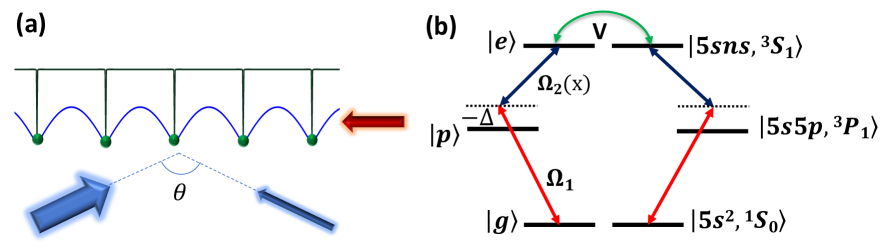
The atomic lattice scheme is based on dressing ${}^{88}Sr$ atoms with the highly excited Rydberg level, see Fig. 1. In the two-photon in-resonance dressing scheme Gau16 ; Kha21 , the single atom Hamiltonian is given by

$${H}_{i}/\hbar=\frac{\Omega_{1}}{2}({\sigma}^{i}_{gp}+{\sigma}^{i}_{pg})+\frac{\Omega_{2}(x_{i})}{2}({\sigma}^{i}_{ep}+{\sigma}^{i}_{pe})-\Delta{\sigma}_{pp},$$ (1)

where $\sigma_{\alpha,\beta}=|\alpha\rangle\langle\beta|$ is the transition operator. The two Rabi frequencies $\Omega_{1,2}$ are applied by 689nm and 318nm lasers that are detuned from the intermediate state ${|{p}\rangle}$ by $\Delta$. With negligible Rydberg decay rates, the system would follow the dark eigen-state $|d\rangle\propto\Omega_{2}|g\rangle-\Omega_{1}|e\rangle$ with zero light-shift. In the limit of $\Omega_{1}\ll\Omega_{2}$, ground state atoms will be partially dressed by Rydberg states with the population of $P_{e}=(\Omega_{1}/\Omega_{2})^{2}$. The van-der Waals interaction between Rydberg atoms ${V}_{ij}=\hbar C_{6}/r_{ij}^{6}{\sigma}_{ee}^{i}{\sigma}_{ee}^{j}$ is a function of interatomic distance $r_{ij}$. This strong interaction could exceed atom-light coupling over several micrometers of interatomic separations.

Figure 2: Interaction-induced atomic lattice. In a simplified picture the first atom is located at the origin, fixed at the node of the standing-wave. (a) The red line shows the spatial profile of the Rabi frequency $\Omega_{2}(x)=\Omega_{2c}+\Omega_{2sw}|\sin(kx\sin(\theta/2))|$, where $k=2\pi/\lambda$. The blue line shows the interaction of two atoms as a function of interatomic distance. When two atoms are within the soft-core radius and are both located at the nodes of the standing wave they experience a strong trapping potential. With a single atom per lattice site, the effective trapping interaction would be the sum of two-body interactions of all the sites within the $\pm R_{c}$ distance. (b) Assuming the first atom to be at the origin, the interaction-induced resonance occurs at the nodes of standing-wave $\Omega_{2}(x_{2})=2|\Delta|$, with the maximum depth of $U_{0}=\frac{\hbar\Omega_{1}^{4}}{8\Delta\gamma^{2}}$ and the HWHM of $\Omega_{2}(x_{2})-2|\Delta|=\pm 2\gamma_{p}$. The analytical form of Eq. 7 and numerical calculation of the interaction potential (Eq. 3) presents a perfect match. (c) Spatial form of the interaction-induced trap for the second atom at the position of the $j^{th}$ standing wave node. The Lorentzian potential of Eq. 5 with the width $w$ (Eq. 6) shows a perfect match with the numeric calculation of Eq. 3. Chosen parameters in (a) are $\Omega_{2c}=2\Delta=2\pi\times 10$MHz, $\Omega_{2sw}=\Delta/2$, maximum loss is limited to 1Hz, $n=100$, $\theta=\pi$.

The dynamic of the system under Rydberg interaction is governed by the master equation of two-body density matrices. The two-body density matrices ${\rho}_{ij}=\text{Tr}_{\bar{i},\bar{j}}{\rho}$ are obtained by tracing over all but $i$ and $j$ particles. The corresponding master equation would be given by

$$\partial_{t}{\rho}_{ij}=-\frac{\text{i}}{\hbar}[{H}_{i}+{H}_{j}+{V}_{ij},{\rho}_{ij}]+\mathcal{L}_{i}({\rho}_{ij})+\mathcal{L}_{j}({\rho}_{ij})$$ (2)

The internal state dynamics are governed by single-particle dissipation described by $\mathcal{L}_{i}$ operator acting on $i$th atom. The Liouvillian term $\mathcal{L}_{i}(\rho)=\sum_{\beta}\mathcal{D}(c_{\beta})\rho_{i}$ with $\mathcal{D}(c)\rho_{i}=c\rho_{i}c^{\dagger}-1/2(c^{\dagger}c\rho_{i}+\rho_{i}c^{\dagger}c)$ in the Lindblad form governs the dissipative time evolution. Lindblad terms encounter spontaneous emission from Rydberg $c_{pe}=\sqrt{\gamma_{e}}|p\rangle\langle e|$ and intermediate level $c_{gp}=\sqrt{\gamma_{p}}|g\rangle\langle p|$. The spontaneous emission rates are $\gamma_{p}/2\pi=7.6$kHz and $\gamma_{e}$ can be found in Kun93 .

Considering the steady state $\bar{\rho}_{ij}$ of Eq. 2, the effective interaction would be given by

$${U}(r_{ij})=\text{Tr}[\bar{\rho}_{ij}({H}_{i}+{H}_{j}+{V}_{ij})].$$ (3)

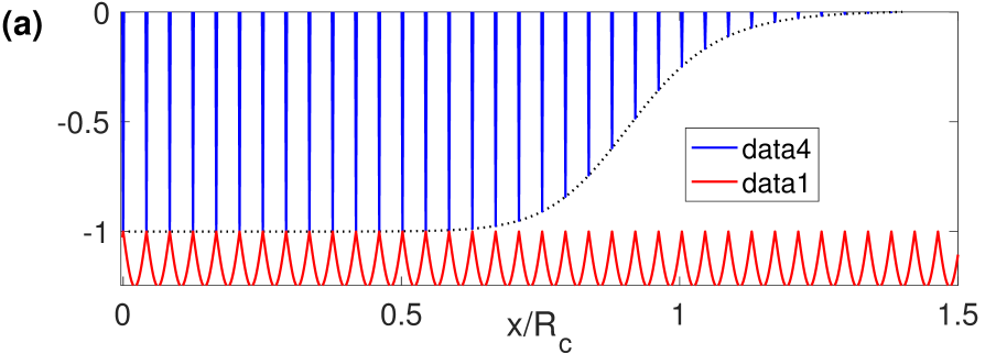
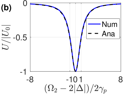
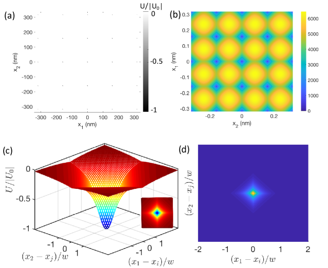
For homogeneous lasers, a plateau-type interaction profile would be formed with constant interaction within the soft-core as depicted by the dotted line in Fig. 2a. In Rydberg-dressing the interaction region is defined by $R_{c}$; the interatomic distance within which interaction-induced laser detuning equals the effective laser bandwidth $P_{r}V(R_{c})=\Omega_{1}\Omega_{2}/2\Delta$ Kha21 . The soft-core interaction features a sharp peak at $\Omega_{2}=2|\Delta|$, due to an interaction-induced resonance, see Fig. 2b.

To form the optical lattice with the mentioned interaction-induced resonance, a space-dependent variation of the upper laser is deployed. Using different intensities for the counter-propagating 318nm lasers, results in the desired spatial pattern of the Rabi frequency

$$\Omega_{2}(x)=\Omega_{2c}+\Omega_{2sw}|\sin(kx\sin(\theta/2))|,$$ (4)

where $k=2\pi/\lambda$ is the laser wave-vector and $\theta$ is the angle between counter propagating lights, see Fig. 1a. Adjusting $\Omega_{2c}=-2\Delta$ in Eq. 4 forms periodic trapping potentials at the nodes of standing wave upon the presence of at least two atoms within the core radius $R_{c}$.

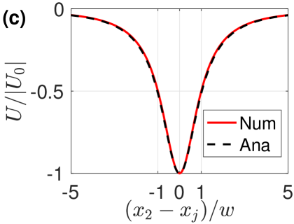
To give a simplified picture of trapping, we initially assume that one atom is fixed at the origin. The trapping potential at the position of the standing nodes are plotted in Fig. 2a,c. Considering the spatial variation of the $\Omega_{2}$ in Eq. 4 over the narrow area $k.(x_{2}-x_{j})\ll 1$ around the $j^{th}$ node of the standing wave, the trapping profile could be approximated by a Lorentzian function

$$U=\frac{U_{0}}{1+(x_{2}-x_{j})^{2}/w^{2}}$$ (5)

where the half-width at half-maximum and the depth of the spatial trap well are given by

$$w=\frac{2\gamma_{p}}{k\sin(\theta/2)\Omega_{2sw}};\quad\quad\quad\quad U_{0}=\frac{\hbar\Omega_{1}^{4}}{8\Delta\gamma^{2}}.\quad\quad\quad$$ (6)

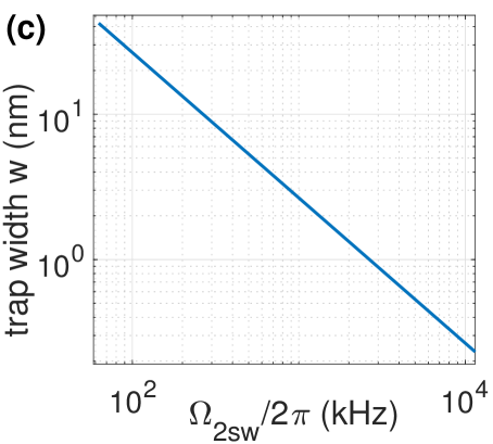
Figure 2c compares this analytical form of Eq. 5 with the numerical results obtained from Eq. 3. The scale of the trap width as a function of $\Omega_{2sw}$ is plotted in Fig. 5c. Remarkably, with $\Omega_{2sw}/2\pi=1.7$MHz the trap width would be as tight as the radius of ⁸⁸Sr atoms.

Note that while the trapping potential exists for overlapping atoms at the origin in Fig. 2a, the collisional blockade mechanism at extremely small trapping volume Sch01 ; Sch02 ensures deterministic single atom loading per lattice site. In a 1D lattice with single atom occupation per site, the effective potential experienced by each site is the sum of two-body interactions of neighbouring lattice sites within the interacting range of $\pm R_{c}$. Deploying the isotropic Rydberg interaction of the $S$ orbital, extension to the 3D lattice is trivial.

A more accurate form of the interaction encounters the motion of two interacting atoms in the lattice. This requires encountering separate laser intensities $\Omega_{2}(x_{1})$ and $\Omega_{2}(x_{2})$ for two atoms. Considering the level scheme of Fig. 3a in two-atom basis, the doubly excited Rydberg state asymptotically decouples within the interaction region $R_{c}$ as $V\rightarrow\infty$. Taking into account the remaining states, in the limit of $\Omega_{1}\ll\Omega_{2c}$ the steady state density could be obtained by adding three orders of perturbative corrections to the initial ground state. In the limit of $\gamma_{p}\ll\Delta$ the dressing interaction between two atoms located at $x_{1}$ and $x_{2}$ inside the interaction region $x_{1}-x_{2}<R_{c}$ is given by

$$U(x_{1},x_{2})=\frac{\hbar\Omega_{1}^{4}}{4\Omega_{2}^{2}(x_{1})\Omega_{2}^{2}(x_{2})\Delta}\frac{[8\Delta^{2}(\Omega_{2}^{2}(x_{1})+\Omega_{2}^{2}(x_{2}))-(\Omega_{2}^{2}(x_{1})-\Omega_{2}^{2}(x_{2}))^{2}](\Omega_{2}^{2}(x_{1})+\Omega_{2}^{2}(x_{2})+8\Delta^{2})}{(\Omega_{2}^{2}(x_{1})+\Omega_{2}^{2}(x_{2})-8\Delta^{2})^{2}+64\gamma_{p}^{2}\Delta^{2}}.$$ (7)

The maximum interaction occurs when the denominator is minimized at $\Omega_{2}(x_{1})^{2}+\Omega_{2}(x_{2})^{2}=8\Delta^{2}$. Note that the attractive or repulsive nature of the potential peak is determined by the sign of detuning $\Delta$. The presented analytic model of Eq. 7 perfectly resemble the numerical results, see Fig. 2, 8. Fig. 8d, plots the ground state wave function of two atoms under dressing trap potential of Eq. 7 as a function of the first and second atoms’ positions $x_{1}$ and $x_{2}$. The mean field approach used the imaginary time evolution of the Gross Pitaevski Equation for calculating the ground motional state.

Figure 3: The origin of the trapping potential is the interaction-induced resonance. (a) With $\Omega_{1}\ll\Omega_{2}$ the two-atom Hilbert space would be organized in three subspaces of ground state, single-excitation (green boxes) and double-excitations (yellow box) that are coupled by weak $\Omega_{1}$ laser. (b) The effects of strong coupling $\Omega_{2}$ and interaction $V$ could be observed by diagonalizing the green and yellow subspaces with eigen-states of $|\beta_{i\pm}\rangle$ and $|\lambda_{0,1,\pm}\rangle$ respectively. The interaction-induced level shift, makes the $|\lambda_{-}\rangle$ in-resonance with the ground state at positions with $\Omega_{2}(x_{1})^{2}+\Omega_{2}(x_{2})^{2}=8\Delta^{2}$. This resonance significantly enhances the interaction and forms the trapping potential.

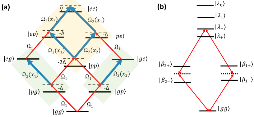
The origin of the enhanced interaction can be traced to a two-atom resonance that occurs in the presence of strong interaction. Considering the laser coupling of two interacting atoms plotted in Fig. 3, for $\Omega_{1}\ll\Omega_{2}$ the two-atoms Hilbert space would be organized in three subspaces that are coupled by weak $\Omega_{1}$ laser. These subspaces are the ground state ${|{gg}\rangle}$, one atom excitation {${|{gp,pg}\rangle}$, ${|{ge,eg}\rangle}$}, and two atom excitation states {${|{pp}\rangle}$, ${|{pe,ep}\rangle}$, ${|{ee}\rangle}$}. The strong coupling $\Omega_{2}$, mixes the states in each subspace. Pre-diagonalizing the subsystems quantifies the light-shifts experienced by the eigen-states, see Fig. 3b. For the second subspace with single excitation in $i^{th}=\{1,2\}$ atom, the coupling Hamiltonian in the {${|{gp}\rangle}$, ${|{ge}\rangle}$} or {${|{pg}\rangle}$, ${|{eg}\rangle}$} basis is given by

$$S_{2}^{i}/\hbar=\begin{pmatrix}-\Delta&\Omega_{2}(x_{i})/2\\ \Omega_{2}(x_{i})/2&0\end{pmatrix}.$$ (8)

The eigen-energies in this subspace $\beta_{i_{\pm}}/\hbar=-\Delta/2\pm 1/2\sqrt{\Delta^{2}+\Omega_{2}(x_{i})^{2}}$ does not get resonant with the ground state. The coupling Hamiltonian in the third subspace with double excitation basis {${|{pp}\rangle}$, ${|{pe}\rangle}$, ${|{ep}\rangle}$, ${|{ee}\rangle}$} is given by

$$\frac{S_{3}}{\hbar}=\begin{pmatrix}-2\Delta&\Omega_{2}(x_{1})/2&\Omega_{2}(x_{2})/2&0\\ \Omega_{2}(x_{1})/2&-\Delta&0&\Omega_{2}(x_{1})/2\\ \Omega_{2}(x_{2})/2&0&-\Delta&\Omega_{2}(x_{2})/2\\ 0&\Omega_{2}(x_{1})/2&\Omega_{2}(x_{2})/2&V\\ \end{pmatrix}$$ (9)

For large interaction inside the soft-core $V\rightarrow\infty$, the eigen-energies are $\lambda_{0}=\hbar V$, $\lambda_{1}=-\hbar\Delta$ and $\lambda_{\pm}=-\frac{3\hbar}{2}\Delta\pm\hbar/2\sqrt{\Delta^{2}+\Omega_{2}(x_{1})^{2}+\Omega_{2}(x_{2})^{2}}$. The doubly excited Rydberg state ${|{\lambda_{0}}\rangle}\approx{|{ee}\rangle}$ decouples asymptotically. At $\Omega_{2}(x_{1})^{2}+\Omega_{2}(x_{2})^{2}=8\Delta^{2}$ one of ${|{\lambda_{\pm}}\rangle}$ eigen-states couples resonantly with the ground state, generating an enhanced light-shift. As discussed above, a small deviation of laser intensity $\Omega_{2}(x_{1})^{2}+\Omega_{2}(x_{2})^{2}-8\Delta^{2}=\gamma_{p}^{2}$ breaks the resonance. Hence, the interaction-induced resonant peaks would be localized at very specific points of the $\Omega_{2}(x)$ standing-wave. This resonance condition generates a bipartite motional correlation, where the atoms oscillate in phase or out of phase, see Fig. 8 and Supp. This would generate a phononic bus that could resemble the atomic version of ion trap gates Cir95 by driving the side-band transitions.

Figure 4: Rydberg dressed trapping - Spatial correlation. (a) Having both atoms free to move, the trapping potential is numerically evaluated from Eq. 3 as a function of the two atoms’ positions $x_{1}$ and $x_{2}$. (b) The resonance condition $(\Omega_{2}(x_{1})^{2}+\Omega_{2}(x_{2})^{2}-8\Delta^{2})/\Gamma_{p}$ is plotted which resembles the potential pattern of (a). (c) The zoomed-in picture of trap potential for the case of two atoms being at $x_{i}$ and $x_{j}$ nodes shows the correlation between atoms’ thermal motion. (inset) The centered diamond equipotential lines force the two atoms to oscillate in phase or out of phase, see Supp. This phononic bus provides all to all connectivity in a multi-dimensional lattice for applying quantum gates via side-band laser driving similar to ion-trap counterparts. (d) Applying the mean-field approach, the two atoms’ ground state wave-function at specific lattice site $x_{j}$ and $x_{j}$ is plotted. Laser parameters are presented in Fig. 2.

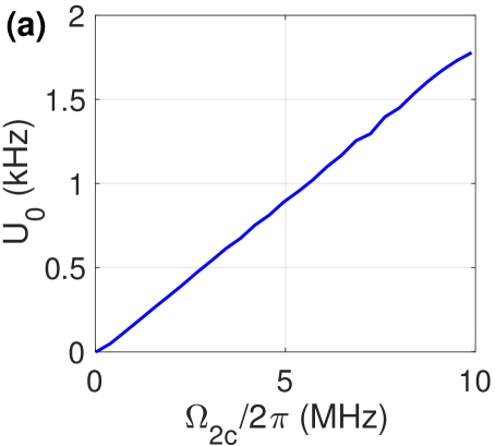
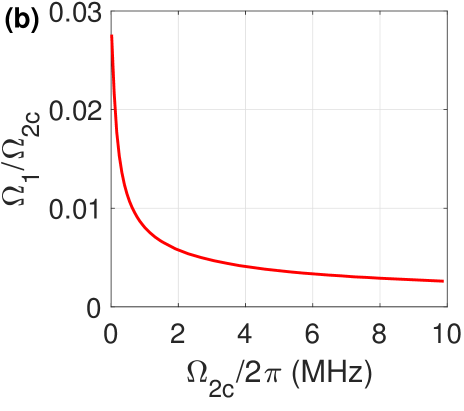
The main source of decoherence in the proposed lattice is the spontaneous emission from the intermediate state. Rydberg interaction disturbs individual atom’s dark state, populating the intermediate state $|p\rangle$, and hence increases the loss rate per atom $\Gamma=\text{Tr}[{\rho}_{i}(\gamma_{p}{\sigma}_{pp}+\gamma_{e}{\sigma}_{ee})]$ at the trapping potential teeth. The loss rate spatial profile follows the interaction profile $\gamma_{p}U_{i,j}(x_{1},x_{2})/\Delta$ since at the resonance points the doubly excited states in the third subspace Eq. 9 would get in resonance with the laser and enhance the population of the short lived $p$ states. The maximum loss for a given $\Omega_{2}(x)$ profile could be controlled by adjusting the intensity of $\Omega_{1}$ laser. The scale of trap depth for two atoms located within the soft-core is plotted in Fig. 5a as a function of $\Omega_{2c}$ for the constant scattering rate of 1Hz at the center of the trap site. The interaction-to-loss ratio enhances by applying stronger laser driving of $\Omega_{2c}$. Having $N$ single-atom-occupied trapping sites within the $\pm R_{c}$ interaction distance, the trapping potential experienced by an atom would add up to $NU_{0}$. In a case study, considering the lattice constant of $\lambda/2$, dressing ground state atoms to ${|{5s100s\,^{3}S_{1}}\rangle}$ with $\Omega_{2c}/2\pi=10$MHz and limiting the loss rate per atom to 1Hz, the collective trapping potential experienced by a single atom in 1D (3D) lattice interacting by neighboring sites within the soft-core would be $N_{1D}U_{0}=77$kHz, ($N_{3D}U_{0}$=37MHz). The benign effects of other decoherence sources are discussed in the Supp.

Figure 5: (a) The scale of trap depth $U_{0}$ for two atoms located within the core distance of $R_{c}$ is plotted as a function of $\Omega_{2c}$ for the constant scattering rate of 1Hz. Having $N$ lattice sites within the interaction distance $R_{c}$, the trapping potential experienced by an atom would add up to $NU_{0}$. (b) The decoherence rate is adjusted to 1Hz by controlling the ratio of $\Omega_{1}/\Omega_{2c}$. (c) The width of Lorentzian traps $w$ (Eq. 6) is plotted as a function of $\Omega_{2sw}$ for $\theta=\pi$.

Outlook- The sub-nanoscale resolution in trapping atoms demonstrated here extends the toolbox of neutral atom quantum technology. The motional correlation forms a phononic bus for quantum computation with all to all connectivity similar to the ion trap with the major advantage of not being restricted to one dimension lattice. Ultra-narrow wells in this proposal allow significant suppression of the lattice constant with a time-sharing approach Nas15 . In this approach, the applied standing wave is stroboscopically shifted in space by $\lambda/2N$ and hence the effective lattice constant would be smaller by a factor of $N^{-1}$. This compaction of the atomic lattice is quite demanding for scaling the lattice sites with the currently limited laser powers. Furthermore, in quantum simulation with optical lattices, the energy scale of Hubbard models for both hopping and interaction of atoms is set by the minimum lattice constant which used to be limited to $\lambda/2$, leading to challenging temperature requirements to observe quantum phases of interest Gro17 .

A distinct research avenue looks at the applications of the presented scheme with ultra-narrow repulsive peaks. Equation 7 shows that changing the detuning sign would preserve the interaction profile but only flip the potential sign from attractive to repulsive. These ultra-narrow barriers are ideal for the realization of the Kronig-Penney (KP) lattice model Kro93 . Furthermore, the three-dimensional repulsive $\delta$-function peaks form nearly perfect box-traps Gau13 . These repulsive narrow peaks also realize thin tunnel junctions for atomtronic devices Sea07 ; Eck14 . The potential is easily generalizable to other geometries in three dimensions using the holographically designed laser intensity Bar18 .

I Supplemental Materials for “An optical-lattice with ultra-narrow trapping teeth featuring phononic bus in multi-dimensional geometry”

I.1 Effects of Collective Many-body Decoherence

Black body radiation (BBR) induced transitions to adjacent Rydberg levels (see Fig.  6a) lead to collective decoherence Zei162 ; Gol16 ; Ama16 . The resonant dipolar interaction between the target Rydberg level $nS$ and the neighboring $n^{\prime}P$ levels causes an anomalous broadening Gol16 . The aforementioned decoherence process is initiated only after the first BBR-induced transition. The Rydberg dressing experiment Zei162 shows that when the perseverance probability of the $nS$ Rydberg level is high enough (of the order of $P_{BBR}(0)=\exp(-P_{r}\Gamma_{BBR}\tau)\geq 82\%$ Zei162 , with $P_{r}=N\Omega_{1}^{2}/\Omega_{2c}^{2}$ being the population of Rydberg state in the entire lattice) the collective decoherence effects are negligible and decoherence rate is dominated by the normal Rydberg depopulation rate.

Figure 6: Collective decoherence. a) BBR-induced transition rates from $|5s100s\,^{3}S_{1}\rangle$ to the neighboring $|5snp\,^{3}P_{2}\rangle$ (dark red), $|5snp\,^{3}P_{1}\rangle$ (pink), $|5snp\,^{3}P_{0}\rangle$ (red) states at the room temperature $T=300$K. The inset is a 20-times magnified image. The resonant interaction between neighboring $P$ states and the original $S$ results in a collective line broadening. (b) The operation time over which the collective decoherence is benign for different environment temperatures.

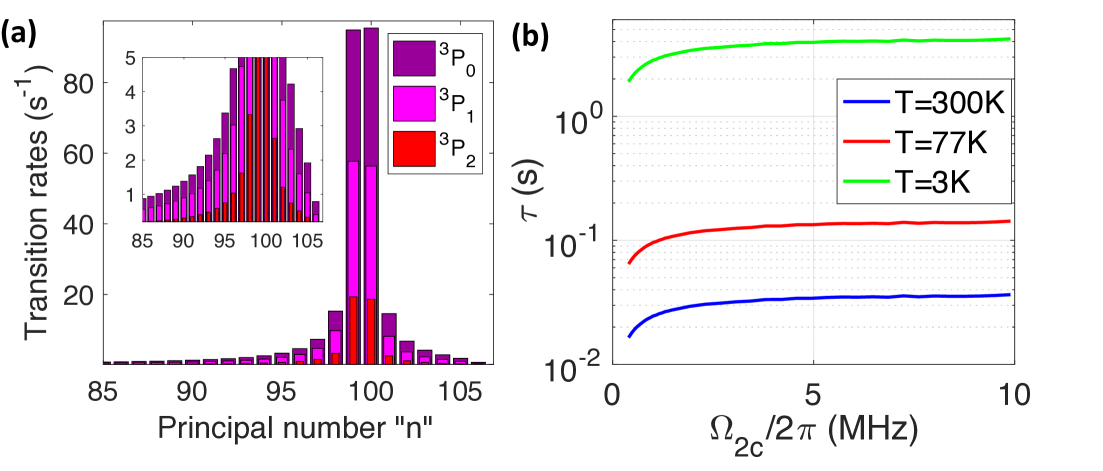
For the targeted Rydberg state ${|{5s100s^{3}S_{1}}\rangle}$ the black-body induced depopulation rate is $\Gamma_{BBR}=1960,\,500,\,17$s^-1, at room temperature $T=300$K and for cryogenic environments 77K and 3K respectively. Fig. 6b completes the Fig. 5 of the main text. It plots the time scale below which the collective decoherence is negligible i.e. $P_{BBR}(0)>0.82$ for different environment temperatures.

I.2 Level Mixing

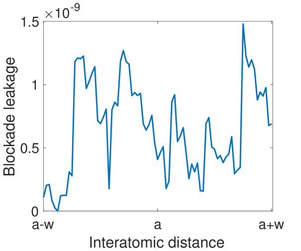
While in the main text, a simplified van-der Waals interaction is considered, a more realistic case must encounter a huge manifold of dipole-coupled Rydberg pairs. The main role of interaction is to block the two Rydberg excitations while the lattice pattern of trapping potential is generated by the variation of the laser intensity. Here the blockade perseverance under strong level mixing is quantified for two neighboring atoms in the lattice. Figure 7 plots the population of two Rydberg excitations considering a manifold of 3800 strongly coupled Rydberg pairs with principal and angular quantum numbers being in the range of $n\in[99-101]$, $l\in[0-2]$. The simulation is performed on two atom basis under the Hamiltonian

$$H=\Omega/\sqrt{2}(|gg\rangle\langle r_{0}g^{+}|+h.c.)+\Omega/\sqrt{2}(|r_{0}g^{+}\rangle\langle r_{0}r_{0}|+h.c.)$$

$$+\sum_{i,j,k,l}\frac{C_{3_{ij,kl}}(\theta)}{R^{3}}(|r_{l}r_{k}\rangle\langle r_{i}r_{j}|+h.c.)+\sum_{i,j}\delta_{ij}|r_{i}r_{j}\rangle\langle r_{i}r_{j}|$$

where the first line excites double Rydberg excitation via the intermediate symmetric state ${|{r_{0}g^{+}}\rangle}=({|{r_{0}g}\rangle}+{|{gr_{0}}\rangle})/\sqrt{2}$ with ${|{r_{0}}\rangle}={|{5s100s\,^{3}S_{1}}\rangle}$. Here the effective Rabi frequency in two-photon transition at the position of lattice sites is given by $\Omega_{t}=\frac{\Omega_{1}\Omega_{2c}}{2\Delta}$. The dipolar interaction $C_{3_{ij,kl}}/{R^{3}}$ mixes a manifold of Rydberg pairs ${|{r_{i}r_{j}}\rangle}$ that are detuned in energy from the initial targeted pair ${|{r_{0}r_{0}}\rangle}$ by $\delta_{ij}$.

Fig. 7 depicts the perseverance of blockade despite strong level mixing between two neighboring lattice sites. This is due to the weak coupling of the molecular resonances to the Rydberg excitation laser which traces back to the diluteness of the optically accessible Rydberg pairs in the manifold of 3800 pair states. At ultra-short distances below the LeRoy radius, the dipolar approximation does not give a complete picture of the interaction, however, ultra-strong interaction assures the absence of double excitation due to the extreme line broadening. This fact has also been proved by blockade experiments in dense atomic ensembles Pey12 ; Dud12 ; Rip18 ; Ome20 ; Shi22 and in the dressing experiment at the range of strong level mixing level mixing 3 .

Figure 7: Rydberg blockade leakage at the position of two neighboring lattice sites under strong level mixing. The manifold of 3800 strongly coupled Rydberg pairs are considered with principal and angular quantum numbers being in the range of $n\in[99-101]$, $l\in[0-2]$. Targets dressed Rydberg state is $|5s100s\,^{3}S_{1}\rangle$ with laser arrangements discussed in Fig. 2. The lattice constant and the trap width are shown by $a$ and $w$.

I.3 Correlated atomic motion

Figure 8: Spatial correlation. (a,b) The trapping potential is presented for the standing wave of the form $\Omega_{2}(x)=4/5\Omega_{2c}+\Omega_{2c}|\sin(k*x)|$ with $\Omega_{2c}=2|\Delta|$. This case presents a diamond ring trapping cross-section that presents the spatial correlation in a more clear way. This correlation forms a phononic bus that could be used in quantum computation via the side-band transition. Fig (c) plots the resonance condition $(\Omega_{2}(x_{1})^{2}+\Omega_{2}(x_{2})^{2}-8\Delta^{2})/\gamma_{p}$ where the resonant regions are shown in blue. Applied parameters are $k=2\pi/318nm^{-1}$; $\Delta=2\pi\times 10$MHz.

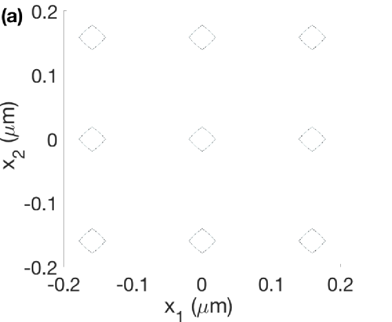
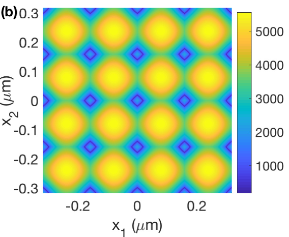
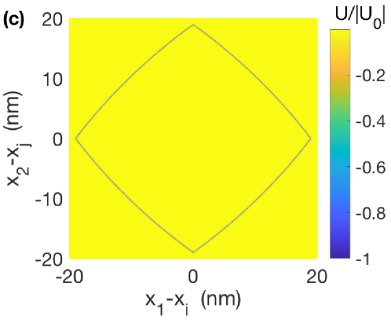
To give a better explanation of the spatial correlation Fig. 8 presents the trapping potential for the standing wave of the form $\Omega_{2}(x)=1.6\Delta+2\Delta|\sin(k*x)|$. This figure presents a more clear picture of two atoms spatial correlation. This correlation provides a phononic bus that couples the vibration of different sites and allows gate operations using side-band laser excitation.

Unlike the ion trap, the phononic bus is not limited to the 1D lattice geometry. Note that the role of interaction is to block the double Rydberg excitation while the shape of potential is determined by the standing-wave pattern of $\Omega_{2}$. Hence by forming 3D standing wave of the form $\Omega_{2}(x,y,z)=\Omega_{2c}+\Omega_{2s}|\sin(kx)\sin(ky)\sin(kz)|$, the same spatial correlation of Fig. 8c that is presented in one dimension between $x_{1}-x_{i}$ and $x_{2}-x_{j}$ would be applied to radial correlation between ${\bf r}_{1}-{\bf r}_{i}$ and ${\bf r}_{2}-{\bf r}_{j}$ for the two sites centred at ${\bf r}_{i}$ and ${\bf r}_{j}$. The resonance condition in three dimension would be given by $\Omega_{2}({\bf r}_{1})^{2}+\Omega_{2}({\bf r}_{2})^{2}=8\Delta^{2}$. Hence the phononic bus that is limited in the ion trap to a one-dimensional lattice could be extended to any two atoms in a multi-dimensional lattice in the presented neutral atom platform. This would be an important step for the scalability of quantum processors that features all to all connectivity.

Supplementary References

J. Zeiher, R. van Bijnen, P. Schauß, S. Hild, J. Choi, T. Pohl, I. Bloch, and C. Gross, Nature Physics 12, 1095 (2016)

E. A. Goldschmidt, T. Boulier, R. C. Brown, S. B. Koller, J. T. Young, A. V. Gorshkov, S. L. Rolston, and J. V. Porto, Phys. Rev. Lett. 116, 113001 (2016).

J. A. Aman, et al. Trap losses induced by near-resonant Rydberg dressing of cold atomic gases, Physical Review A 93, 043425 (2016).

Peyronel, T., Firstenberg, O., Liang, Q.-Y., Hofferberth, S., Gorshkov, A. V., Pohl, T., Lukin, M. D., and Vuletic, V., ”Quantum nonlinear optics with single photons enabled by strongly interacting atoms”, Nature 488, 57-60 (2012).

Dudin, Y.O. and Kuzmich, A., ”Strongly interacting Rydberg excitations of a cold atomic gas,” Science, 336(6083), 887-889 (2012).

Ripka, F., Kübler, H., Löw, R. and Pfau, T., ”A room-temperature single-photon source based on strongly interacting Rydberg atoms,” Science, 362(6413), 446-449 (2018).

Ornelas-Huerta, D.P., Craddock, A.N., Goldschmidt, E.A., Hachtel, A.J., Wang, Y., Bienias, P., Gorshkov, A.V., Rolston, S.L. and Porto, J.V., ”On-demand indistinguishable single photons from an efficient and pure source based on a Rydberg ensemble,” Optica, 7(7), 813-819 (2020).

Shi, S., Xu, B., Zhang, K., Ye, G.S., Xiang, D.S., Liu, Y., Wang, J., Su, D. and Li, L., ”High-fidelity photonic quantum logic gate based on near-optimal Rydberg single-photon source,” Nature Comms. 13(1), 4454 (2022).

Y.Y. Jau, A. M. Hankin, T. Keating, I. H. Deutsch, and G. W. Biedermann, arXiv:1501.03862 (2015).

Khazali, Mohammadsadegh, and Wolfgang Lechner. ”Electron cloud design for Rydberg multi-qubit gates.” arXiv preprint arXiv:2111.01581 (2021).

References

- (1) M. Khazali, W. Lechner, Scalable quantum processors empowered by the Fermi scattering of Rydberg electrons. Comms. Phys. 6, 57 (2023).
- (2) Khazali, Mohammadsadegh, Universal terminal for mobile edge-quantum computing, arXiv:2204.08522 (2022).
- (3) M. Khazali, Discrete-Time Quantum-Walk & Floquet Topological Insulators via Distance-Selective Rydberg-Interaction, Quantum 6, 664 (2022).
- (4) Hollerith, S., Srakaew, K., Wei, D., Rubio-Abadal, A., Adler, D., Weckesser, P., Kruckenhauser, A., Walther, V., van Bijnen, R., Rui, J. and Gross, C., Realizing distance-selective interactions in a Rydberg-dressed atom array. Phys. Rev. Lett., 128, 113602 (2022).
- (5) C. Ates, T. Pohl, T. Pattard, and J. M. Rost, ”Antiblockade in Rydberg excitation of an ultracold lattice gas.” Phys. Rev. Lett. 98, 023002 (2007).
- (6) Graham, T.M., Kwon, M., Grinkemeyer, B., Marra, Z., Jiang, X., Lichtman, M.T., Sun, Y., Ebert, M. and Saffman, M., Rydberg-mediated entanglement in a two-dimensional neutral atom qubit array. Phys. Rev. lett., 123, 230501 (2019).
- (7) A. Pagano, S. Weber, D. Jaschke, T. Pfau, F. Meinert, S. Montangero, and H. P. Büchler, Error budgeting for a controlled-phase gate with strontium-88 Rydberg atoms, Phys. Rev. Research 4, 033019 (2022).
- (8) Cetina, M., Egan, L.N., Noel, C., Goldman, M.L., Biswas, D., Risinger, A.R., Zhu, D. and Monroe, C., Control of transverse motion for quantum gates on individually addressed atomic qubits. PRX Quantum, 3, 010334 (2022).
- (9) Brennen, G.K., Caves, C.M., Jessen, P.S. and Deutsch, I.H., Quantum logic gates in optical lattices. Phys. Rev. Lett. 82, 1060 (1999).
- (10) Cirac, Juan I., and Peter Zoller. ”Quantum computations with cold trapped ions.” Phys. Rev. Lett. 74(20), 4091 (1995).
- (11) M. Saffman, T. G. Walker, and K. Mølmer. ”Quantum information with Rydberg atoms.” Rev. Pod. Phys. 82, 2313 (2010).
- (12) M. Khazali and K. Mølmer. Fast multiqubit gates by adiabatic evolution in interacting excited-state manifolds of Rydberg atoms and superconducting circuits. Phys. Rev. X, 10, 021054, (2020).
- (13) M. Khazali, C. R Murray, and T. Pohl. Polariton exchange interactions in multichannel optical networks. Phys. Rev. Lett., 123 113605, 2019.
- (14) M. Khazali, K. Heshami, and C. Simon. Photon-photon gate via the interaction between two collective Rydberg excitations. Physical Review A, 91 030301, (2015).
- (15) M. Khazali, ”All-optical quantum information processing via a single-step Rydberg blockade gate” Opt. Express 31(9), 13970-13980 (2023).
- (16) M. Khazali, K. Heshami, and C. Simon. Single-photon source based on Rydberg exciton blockade. J. Phys. B: At. Mol. Opt. Phys., 50, 215301, (2017).
- (17) M. Khazali, ”Quantum information and computation with Rydberg atoms.” Iranian Journal of Applied Physics 10 19 (2021); M. Khazali, Applications of Atomic Ensembles for Photonic Quantum Information Processing and Fundamental Tests of Quantum Physics. Diss. University of Calgary (Canada), (2016).
- (18) J. Zeiher, R. Van Bijnen, P. Schaus, S. Hild, J. Choi, T. Pohl, I. Bloch, and C. Gross. ”Many-body interferometry of a Rydberg-dressed spin lattice.” Nature Physics 12, 1095-1099 (2016).
- (19) Hines, J. A., Rajagopal, S. V., Moreau, G. L., Wahrman, M. D., Lewis, N. A., Markovi, O., & Schleier-Smith, M. Spin Squeezing by Rydberg Dressing in an Array of Atomic Ensembles. arXiv:2303.08805 (2023).
- (20) Eckner, William J., Nelson Darkwah Oppong, Alec Cao, Aaron W. Young, William R. Milner, John M. Robinson, Jun Ye, and Adam M. Kaufman. ”Realizing spin squeezing with Rydberg interactions in a programmable optical clock.” arXiv:2303.08078 (2023).
- (21) M. Khazali, H. W. Lau, A. Humeniuk, and C. Simon. Large energy superpositions via Rydberg dressing. Phys. Rev. A, 94, 023408, (2016);
- (22) M. Khazali. Progress towards macroscopic spin and mechanical superposition via Rydberg interaction. Phys. Rev. A, 98, 043836, (2018).
- (23) Santos, L., Shlyapnikov, G. V., Zoller, P., & Lewenstein, M. Bose-Einstein condensation in trapped dipolar gases. Physical Review Letters, 85, 1791 (2000).
- (24) Honer, J., Weimer, H., Pfau, T., & Büchler, H. P. Collective many-body interaction in Rydberg dressed atoms. Physical review letters, 105, 160404 (2010).
- (25) C. Gaul, B. J. DeSalvo, J. A. Aman, F. B. Dunning, T. C. Killian, and T. Pohl, Resonant Rydberg Dressing of Alkaline-Earth Atoms via Electromagnetically Induced Transparency, Phys. Rev. Lett. 116, 243001 (2016).
- (26) M. Khazali, Rydberg noisy dressing and applications in making soliton molecules and droplet quasicrystals, Phys. Rev. Research 3, L032033 (2021)
- (27) Henkel, N., Cinti, F., Jain, P., Pupillo, G. and Pohl, T., Supersolid vortex crystals in Rydberg-dressed Bose-Einstein condensates. Physical Review Letters 108,265301 (2012).
- (28) S. Kunze, R. Hohmann, H. J. Kluge, J. Lantzsch, L. Monz, J. Stenner, K. Stratmann, K. Wendt, and K. Zimmer, Lifetime measurements of highly excited Rydberg states of strontium I, Z. Phys. D 27, 111 (1993).
- (29) N. Schlosser, G. Reymond, I. Protsenko, and P. Grangier, Nature London 411, 1024 2001.
- (30) N. Schlosser, G. Reymond, and P. Grangier, Phys. Rev. Lett. 89, 023005 2002
- (31) S. Nascimbene, N. Goldman, N. R. Cooper, and J. Dalibard, Dynamic optical lattices of sub-wavelength spacing for ultracold atoms, Phys. Rev. Lett. 115, 140401 (2015).
- (32) C. Gross and I. Bloch, Science 357, 995 (2017).
- (33) R. de L. Kronig and W. G. Penney, Proc. Roy. Soc. A 130, 499 (1931).
- (34) A. L. Gaunt, T. F. Schmidutz, I. Gotlibovych, R. P. Smith, and Z. Hadzibabic, Bose-Einstein condensation of atoms in a uniform potential, Phys. Rev. Lett. 110, 200406 (2013).
- (35) BT. Seaman, M. Krämer, DZ. Anderson, MJ. Holland, ”Atomtronics: Ultracold-atom analogs of electronic devices.” Physical Review A 75, 023615 (2007).
- (36) S. Eckel, J. G. Lee, F. Jendrzejewski, N. Murray, C. W. Clark, C. J. Lobb, W. D. Phillips, M. Edwards, and G. K. Campbell, Hysteresis in a quantized superfluid atomtronic circuit, Nature 506, 200 (2014).
- (37) Barredo, D., Lienhard, V., De Leseleuc, S., Lahaye, T. and Browaeys, A., Synthetic three-dimensional atomic structures assembled atom by atom. Nature 561, 79 (2018).