Comprehensive spectroscopic and photometric study of pulsating eclipsing binary star AI Hya

Abstract

The pulsating eclipsing binaries are remarkable systems that provide an opportunity to probe the stellar interior and to determine the fundamental stellar parameters precisely. Especially the detached eclipsing binary systems with (a) pulsating component(s) are significant objects to understand the nature of the oscillations since the binary effects in these systems are negligible. Recent studies based on space data have shown that the pulsation mechanisms of some oscillating stars are not completely understood. Hence, comprehensive studies of a number of pulsating stars within detached eclipsing binaries are important. In this study, we present a detailed analysis of the pulsating detached eclipsing binary system AI Hya which was studied by two independent groups with different methods. We carried out a spectroscopic survey to estimate the orbital parameters via radial velocity measurements and the atmospheric parameters of each binary component using the composite and/or disentangled spectra. We found that the more luminous component of the system is a massive, cool and chemically normal star while the hotter binary component is a slightly metal-rich object. The fundamental parameters of AI Hya were determined by the analysis of binary variations and subsequently used in the evolutionary modelling. Consequently, we obtained the age of the system as 850 $\pm$ 20 Myr and found that both binary components are situated in the $\delta$ Scuti instability strip. The frequency analysis revealed pulsation frequencies between the 5.5 – 13.0 d^-1 and we tried to estimate which binary component is the pulsating one. However, it turned out that those frequencies could originate from both binary components.

1 Introduction

To understand the universe, it is necessary to comprehend stars which are its building blocks. For a deep investigation of stars, we should know their basic stellar parameters such as mass ($M$), radius ($R$) and chemical composition. Binary stars, in particular the eclipsing ones, are the most suitable objects to derive these parameters as $M$ and $R$ can be derived with an accuracy better than 1% (Torres, Andersen, & Giménez, 2010; Southworth, 2013). Therefore, these systems are substantial for a better understanding of the universe, our Galaxy, and, most directly, stellar evolution. However, eclipsing binary systems as such do not provide information about the stellar interior. This is where the pulsating stars come in. The oscillation frequencies of pulsating stars can be used to probe the stellar interior by applying asteroseismic methods, making eclipsing binary systems with (a) pulsating component(s) one of the most valuable tools to improve our knowledge of stellar evolution.

Various types of pulsating stars in different evolutionary states exist. Some of them, such as $\beta$ Cephei, $\delta$ Scuti, and $\gamma$ Doradus stars (Lampens, 2021; Southworth, 2021), are also found in eclipsing binary systems. The $\delta$ Scuti  variables are the most common pulsating stars found in eclipsing binaries because of their relatively short pulsation periods. The $\delta$ Scuti  stars are A to F-type dwarf or giant stars generally exhibiting pressure mode oscillations with periods between 18 min and 8 h and amplitudes below 0^m.1 in the V-band (Aerts, Christensen-Dalsgaard, & Kurtz, 2010). Their theoretical instability strip (e.g. Dupret et al. 2005) indicates the location of objects in the Hertzsprung-Russell (H-R) diagram that are expected to show $\delta$ Scuti-type oscillations. Thanks to space missions such as Kepler (Borucki et al., 2010) and the Transiting Exoplanet Survey Satellite (TESS, Ricker et al., 2014), we learned that $\delta$ Scuti  stars are also observed beyond the borders of the theoretical instability strip, showing the necessity to revise them (Uytterhoeven et al., 2011; Antoci et al., 2014; Bowman & Kurtz, 2018). According to the latest catalog of $\delta$ Scuti stars in eclipsing binaries, there are around 90 such objects (Kahraman Aliçavuş et al., 2017). This number is now increasing especially by the discoveries of new systems from the investigation of the space data (e.g. Kahraman Aliçavuş et al., 2022; Gaulme & Guzik, 2019). The pulsations of the $\delta$ Scuti  stars in eclipsing binaries are affected by the other binary component (Kahraman Aliçavuş et al., 2017; Liakos & Niarchos, 2017). Indeed, their pulsation period ($P_{\rm puls}$) decreases when the orbital period ($P_{\rm orb}$) becomes shorter and, hence, the other component approaches the pulsating component. It was also thought that the tidal forces between the binary components can alter the pulsation axis (Kurtz et al., 2020). The first observational proof of this was presented by Handler et al. (2020) thanks to the high-quality data of TESS. These authors showed that in some binary systems the pulsation axis can align with the orbital axis because of the tidal forces. This type of object is now known as tidally tilted pulsators and they are a clear proof of binary effects on pulsations.

For a deep understanding of the effects of binarity on pulsations in eclipsing binary systems and on stellar evolution and structure, comprehensive investigations of such systems are necessary. AI Hya (V = 9^m.35) is an eclipsing binary system with a $\delta$ Scuti  component consisting of a F2m and F0V star (Stancliffe et al., 2015). It has an eccentric orbit and an orbital period of 8.289649(2) days (Kreiner, 2004). Spectroscopic observations revealed that AI Hya is a double-lined binary system (Popper, 1988). In a recent study, an updated photometric analysis based on the TESS data of AI Hya was given which shows that the secondary component exhibits multiperiodic oscillations (Lee, Hong, & Kristiansen, 2020). However, no detailed spectral analysis with high-resolution spectra has been carried out for the system so far. Therefore, we provide a detailed photometric and spectral analysis of AI Hya in this study to reveal the true character of this interesting object.

Two teams were working on this system independently. One group was led by TP (group-P with KH, AM, NU, and EK) and the second group by FKA (group-K with GH, FA, PDC, FL, GC, and MG). We used the same photometric but different spectroscopic data. We compared our partial results as the work progressed. However, the overall approach used by each group was different. In the end, we combined our results to obtain the final parameters of the system. The paper is organized as follows. In Sect. 2 the observational data are introduced. The radial velocity and spectral analyses are given in Sect. 3 and Sect. 4, respectively. The binary modelling and the pulsation frequency analysis are presented in Sect. 5 and Sect. 6. In Sect. 7, discussions and conclusions are given.

2 Observational Data

In the photometric analysis of AI Hya, TESS data was used by both groups. TESS was launched in April 2018 mainly to detect new exoplanets (Ricker et al., 2014). TESS has monitored almost the entire sky which has been subdivided into sectors that are observed for about 27 days each. The TESS observations were taken in 2-min. short (SC) and 30-min long (LC) cadence in the nominal phase of the mission (first two years). For the extended mission, the LC was reduced to 10-min. The data are available in the Barbara A. Mikulski Archive for Telescopes (MAST) where they are released in different versions: simple aperture photometry (SAP) and pre-search data conditioning SAP fluxes (PDCSAP). AI Hya was observed in one sector only (sector 7). The 2-min SAP fluxes were used in our analysis since SAP fluxes have lower flux uncertainty and 2-min data are more suitable for the analysis of AI Hya (see Sect. 6). They were converted into magnitude by using the same method as Kahraman Aliçavuş et al. (2022).

Photometric data from ground-based surveys also exist, e.g. from ASAS 3 (Pojmański, 2002) and ASAS-SN (Jayasinghe et al., 2018), but they are of inferior quality and do not allow for proper analysis of pulsations. The TESS sector 7 data are the best ones available so far, although AI Hya will again be visible in the satellite’s field of view in sector 61.

Table 1: Information about the spectroscopic observations. N, R and SNR represent the number of the spectra, resolving power and the signal-to-noise ratio, respectively.

Spectrometer	N	Observations	R	SNR	Spectral
		years			range [Å]
CAOS	1	2021	38000	50	415 $-$ 670
CORALIE	3	2015	60000	20 $-$ 34	390 $-$ 680
HERMES	15	2020	85000	50 $-$ 70	377 $-$ 900
HIDES	13	2014 $-$ 2017	50000	40 $-$ 88	408 $-$ 752

The spectroscopic data of the system were taken from four different instruments. The list of the instruments and the basic information about them are given in Table 1. One spectrum was taken with Catania Astrophysical Observatory Spectropolarimeter (CAOS, Leone, et al., 2016). The CAOS is a high-resolution, fibre-fed, cross-dispersed échelle spectrograph installed to the 91-cm telescope at the Catania Astrophysical Observatory (Mt. Etna, Italy). Three spectra of AI Hya were collected from the CORALIE échelle spectrograph which is mounted on the 1.2-m Leonhard Euler telescope at La Silla Observatory (Chile) (Pepe et al., 2018). The High Efficiency and Resolution Mercator échelle spectrograph (HERMES) was also used to obtain high-resolution spectra of AI Hya. HERMES is mounted on the 1.2-m Mercator telescope at the Roque de Los Muchchos observatory on the Canary Island La Palma in Spain (Raskin et al., 2011). The last instrument used in this study is the HIgh-Dispersion Échelle spectrograph (HIDES). HIDES is attached to the 1.88-m telescope of Okayama astrophysical observatory in Japan (Kambe et al., 2013). The spectra of CORALIE and HIDES were taken by group-P, while the spectra of CAOS and HERMES were gathered by group-K. In total 32 spectra of AI Hya were gathered and these spectra are well distributed in orbital phases of AI Hya. Each group used the obtained spectra to measure the radial velocity ($v_{r}$ ) changes. Additionally, these data were taken into account to derive the atmospheric parameters (e.g. effective temperature $T_{\rm eff}$, surface gravity $\log g$, metallicity) and the projected rotational velocity ($v\sin i$) of the components of AI Hya.

3 Radial Velocity analysis

The $v_{r}$  values of the AI Hya system were measured with different approaches by both group-P and group-K using different spectra taken from the distinct instruments.

3.1 $v_{r}$  measurements

Group-P calculated the $v_{r}$  values from HIDES and CORALIE spectra, using the two-dimensional cross-correlation todcor program (Zucker & Mazeh, 1994). In the analysis, a synthetic spectrum was used as a template and this spectrum was generated using an ATLAS9 model atmosphere (Kurucz, 1993) having $T_{\rm eff}$, metallicity [M/H] and $v\sin i$  parameters of 6800 K, 0.0 and 30 km s^-1, respectively. When a template with 60 km s^-1(the $v\sin i$  value found in further analysis) was used, the results did not improve in terms of $rms$ of the orbital fit, nor did the uncertainties of orbital elements. Moreover, some points, with the smallest difference in $v_{r}$  measurements, seemed to suffer from systematic effects, and had to be rejected. We therefore believe the use of 30 km s^-1templates was justified. The calculated $v_{r}$  values for each binary component are given in Table A1.

Group-K used the RaVeSpAn code (Pilecki et al., 2017) to determine the $v_{r}$  values of the binary components using the broadening function formalism. In the analysis, local thermodynamic equilibrium (LTE) synthetic spectra with atmospheric parameters similar to that of group-P were used as templates (Coelho et al., 2005). The spectra of CAOS and HERMES were used in the $v_{r}$  measurements. The resulting $v_{r}$  measurements are given in Table A1.

3.2 $v_{r}$  curve modelling

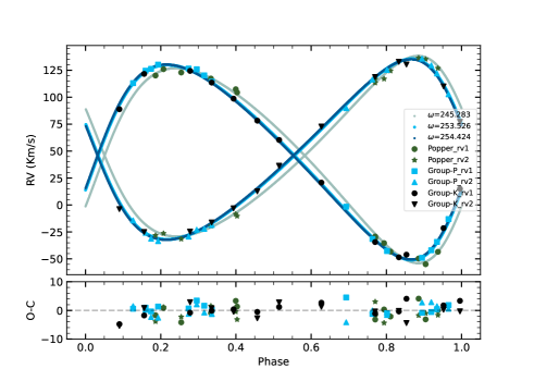
For the spectroscopic orbital fitting, group-P used all the available $v_{r}$  measurements, including those made by group-K and from Popper (1988). Group-P used the v2fit code (Konacki et al., 2010) which adjusts a double-Keplerian with a Levenberg-Marquardt algorithm. In this analysis, the amplitude of $v_{r}$  curves ($K$), $P_{\rm orb}$, the time of phase zero ($T_{0}$), mass centre’s velocity ($\gamma$), eccentricity ($e$) and argument of the periastron ($\omega$) were set as free parameters. Thanks to the long time span of the data ($>$51 years), it was possible to detect the apsidal motion ($\dot{\omega}$) of the binary’s orbit: 0.186(56) deg/yr. This is in reasonable agreement (1.75$\sigma$) with the value given by Lee, Hong, & Kristiansen (2020): 0.075(31) deg/yr. The results of the analysis are given in Table 2 and the theoretical $v_{r}$  curve fits to the measured $v_{r}$  data are illustrated in Fig.1.

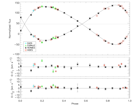
Group-K used the rvfit code for the radial velocity analysis. The rvfit program can analyse single and double-lined binary systems by using the adaptive simulated annealing method (Iglesias-Marzoa et al., 2015). In the analysis, the $P_{\rm orb}$ taken from Kreiner (2004) was considered as a fixed parameter. Other orbital parameters such as $T_{0}$, $K$, $\gamma$, $\omega$ and $e$ were taken as free parameters during the analysis. Both groups $v_{r}$  measurements were used in the analysis and as a result, the orbital parameters of the system were obtained. The resulting parameters of the current $v_{r}$  analysis are given in Table 2. The consistency between the theoretical $v_{r}$  curve and measurements is shown in Fig. 2.

Both groups found the resulting mass ratio ($q=M_{2}/M_{1}=K_{1}/K_{2}$) larger than 1 (1.075 $\pm$ 0.011 and 1.080 $\pm$ 0.007 for groups -K and -P, respectively). According to this $q$ value, the $v_{r}$  curve and the results, the star (generally called secondary) covered by the hotter binary component at orbital phase 0.5 is more massive than the hotter binary component (primary). To test these findings, binary modelling is necessary. Therefore, these results will be tested in the binary modelling sections.

Table 2: The results of the radial velocity analysis. The subscripts 1 and 2 refer to hotter primary and cooler secondary components, respectively. ^a shows the fixed parameters.

Parameter	Group-P	Group-K
$T_{0}$ (HJD)	2458491.570 $\pm$ 0.028	2452506.383 $\pm$ 0.032
$P_{\rm orb}$(d)	8.289761 $\pm$ 0.000027	8.2896490a
$\gamma$ (km/s)	45.90 $\pm$ 0.24	45.70 $\pm$ 0.35
$K_{1}$ (km/s)	90.42 $\pm$ 0.37	89.52 $\pm$ 0.65
$K_{2}$ (km/s)	83.71 $\pm$ 0.46	83.29 $\pm$ 0.63
$e$	0.2419 $\pm$ 0.0036	0.2432 $\pm$ 0.0050
$\omega$ (deg)	254.03 $\pm$ 1.30	250.92 $\pm$ 1.63
$\dot{\omega}$ (deg/yr)	0.186 $\pm$ 0.056
$a_{1}\sin i$ ($R_{\odot}$)	14.380 $\pm$ 0.061	14.222 $\pm$ 0.105
$a_{2}\sin i$ ($R_{\odot}$)	13.312 $\pm$ 0.072	13.233 $\pm$ 0.101
$a\sin i$ ($R_{\odot}$)	27.692 $\pm$ 0.094	27.454 $\pm$ 0.145
$M_{1}\sin^{3}i$ ($M_{\odot}$)	1.992 $\pm$ 0.023	1.950 $\pm$ 0.033
$M_{2}\sin^{3}i$ ($M_{\odot}$)	2.151 $\pm$ 0.022	2.095 $\pm$ 0.035
$q=M_{2}/M_{1}$	1.080 $\pm$ 0.007	1.075 $\pm$ 0.011

Figure 1: Upper panel: The model $v_{r}$  fit to the combined $v_{r}$ measurements from Popper (1988), Group-P (HIDES+CORALIE) and Group-K (HERMES+CAOS). Lower panel: residuals. Model made by Group-P.

Figure 2: Upper panel: The model $v_{r}$  fit to the $v_{r}$  measurements of Groups-K and -P. Lower panel: residuals. Model made by Group-K.

4 Spectral analysis

4.1 Group-K

4.1.1 Spectral disentangling

To obtain the atmospheric parameters ($T_{\rm eff}$, $\log g$), $v\sin i$  and the chemical composition of each binary component of AI Hya, a detailed spectral analysis is necessary. As AI Hya is a double-lined binary system, its spectrum consists of the spectral lines of both binary components. Therefore, group-K carried out a spectral disentangling analysis to extract the individual spectra of each binary component from the composite spectra of AI Hya. In the analysis, the code fdbinary was used (Ilijic et al., 2004). fdbinary is capable of disentangling a composite spectrum, which includes flux contributions from two or three components, in Fourier space. Before the analysis with fdbinary, one should know the light contributions of the binary components at the orbital phases corresponding to the times the spectra were taken. These values should be fixed during the analysis. Hence, to determine the light contributions of both binary components at the different orbital phases, we carried out a preliminary binary modelling of AI Hya by taking $T_{\rm eff}$  of the TESS Input Catalog (TIC; Stassun et al., 2019) as the $T_{\rm eff}$  of the hotter component. The analysis was performed utilizing the Wilson-Devinney code (Wilson & Devinney, 1971). As a result of this preliminary analysis, it was found that the hotter and cooler binary components contribute around 38% and 62% to the total, respectively. However, one should keep in mind that these light contributions change according to the orbital phases. For example, the primary eclipse is a total eclipse where the light contribution of the hotter components is negligible.

In the analysis, we used the HERMES spectra as they are well distributed over the orbital phases and have a higher resolving power. Taking into account the observation time of each HERMES spectrum, the light contributions at these times were first determined using the fluxes measured from the photometric solution and subsequently fixed during the analysis. In addition to this, we also fixed all results derived in the $v_{r}$  analysis during the spectral disentangling. For the disentangling progress, we used the spectral interval of $\sim$4200 $-$ 6400 Å by ignoring the parts polluted by telluric lines. For the analysis, this spectral window was divided into 15 spectral parts with steps of $\sim 100-150$ Å. Each small spectral part was then analysed separately. As a result, we obtained the individual spectra of each binary component. The separated spectra derived with fdbinary were re-normalised by taking into account the light ratio of the binary components, as described by Ilijic et al. (2004).

4.1.2 Determination of the atmospheric parameters and chemical compositions

After the individual spectra of the components of AI Hya were obtained, we were able to determine the atmospheric parameters, $v\sin i$, and the chemical composition. To derive these parameters, we used the plane-parallel and line-blanketed local thermodynamic equilibrium (LTE) ATLAS9 model atmospheres (Kurucz, 1993) and the synthe code (Kurucz & Avrett, 1981) to generate theoretical spectra. First, the hydrogen lines of the binary components were used to obtain initial $T_{\rm eff}$ values.

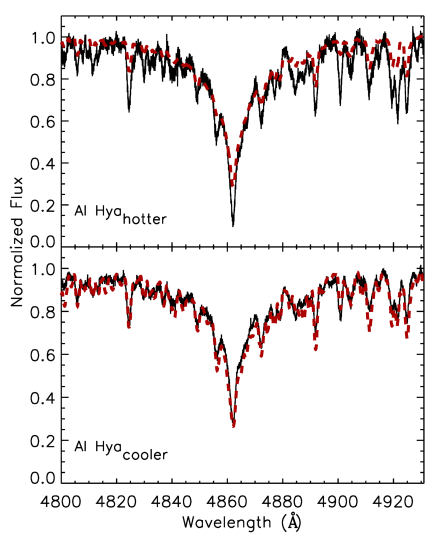
In this analysis, the $H_{\beta}$ lines of the components were compared with many theoretical $H_{\beta}$ lines which were derived for a wide range of $T_{\rm eff}$  ($5000-9000$ K) with a step size of 100 K, where $\log g$  and metallicity were fixed to 4.0 and solar, respectively. During the analysis, we took into account the minimization method described by Catanzaro, Leone, & Dall (2004) and successfully applied in a series of papers (i.e., Catanzaro et al., 2022, 2019). Consequently, the $T_{\rm eff}$  of the hotter and cooler components were found to be 7500 $\pm$ 200 K and 7000 $\pm$ 150 K, respectively. We did not attempt to optimize $\log g$ because the hydrogen lines are not sensitive to this parameter for stars cooler than 8000 K (Smalley et al., 2002). The best theoretical $H_{\beta}$ line fits to the separated spectra of the components are shown in Fig. 3.

Figure 3: Theoretical hydrogen line fits (red dashed lines) to the $H_{\beta}$ lines (solid black line) of the hotter and cooler binary components (Group-K).

We also determined values for $\log g$, the microturbulent velocity $\xi$, and $v\sin i$ by improving the initially determined $T_{\rm eff}$  value using the excitation potential$-$abundance relationship. For the correct atmospheric parameters, different excitation potentials of the same element should give the same abundances. Therefore, by using this relation for iron (Fe), we determined the atmospheric parameters. Detailed information about this analysis method is given by Kahraman Aliçavuş et al. (2016). The results of this analysis are listed in Table 3. To determine the errors on the atmospheric parameters, we checked how their values change for differences in the excitation potential$-$abundance correlation of about 5%.

Figure 4: Consistency between the synthetic (dashed-lines) and disentangled spectra of the components of AI Hya (Group-K).

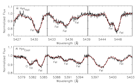
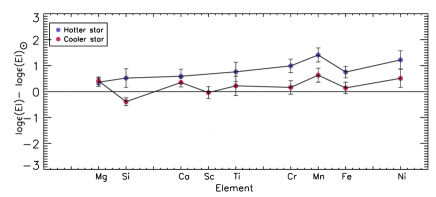
In the next step, the chemical composition of the binary components was derived after fixing the atmospheric parameters to their final values. For the chemical abundance determination, we first identified the lines based on the Kurucz line list. The spectral synthesizing method and the identified lines were used in this examination. Consequently, the chemical compositions of both binary components were obtained and the results are listed in Table 4. The consistency between the synthetic and observed spectra of both binary components is illustrated in Fig. 4. The abundance distributions relative to solar abundance (Asplund et al., 2009) are shown in Fig. 5, indicating that the hotter binary component has an overabundance compared to the Sun for some elements. The errors of the chemical compositions were determined including the uncertainties in the derived atmospheric parameters and the effects of the resolving power and the SNR of the spectra, as described by Kahraman Aliçavuş et al. (2016).

Table 3: The final atmospheric parameters and $v\sin i$ value of the hot (primary) and cool binary components of AI Hya. $\log\epsilon$ (Fe) represent the relative abundance with respect to hydrogen (H=12.0)

.  Group-K $T_{\rm eff}$ (K) $\log g$ (cgs) $\xi$ (km s^-1) $v\sin i$ (km s^-1) $\log\epsilon$ (Fe) Primary 7700 $\pm$ 100 3.8 $\pm$ 0.1 3.4 $\pm$ 0.3 57 $\pm$ 6 8.25 $\pm$ 0.54 Secondary 7200 $\pm$ 100 3.6 $\pm$ 0.2 1.9 $\pm$ 0.3 64 $\pm$ 4 7.64 $\pm$ 0.20  Group-P (gssp) $T_{\rm eff}$ (K) $\log g$ (cgs) $\xi$ (km s^-1) $v\sin i$ (km s^-1) $\mathrm{[M/H]}$ Primary 7350 $\pm$ 300 3.8 (fixed) 4.83 $\pm$ 1.15 50 (fixed) 0.14 $\pm$ 0.14 Secondary 7150 $\pm$ 250 3.6 (fixed) 3.07 $\pm$ 0.52 62 (fixed) 0.06 $\pm$ 0.10  Group-P (iSpec) $T_{\rm eff}$ (K) $\log g$ (cgs) $\xi$ (km s^-1) $v\sin i$ (km s^-1) $\mathrm{[M/H]}$ Primary 7300 $\pm$ 170 3.83 (fixed) 5.33 $\pm$ 0.86 50 (fixed) 0.15 (fixed) Secondary 7260 $\pm$ 175 3.58 (fixed) 3.98 $\pm$ 0.70 62 (fixed) 0.01 (fixed)

Table 4: Abundances of individual elements of the binary components and Sun (Asplund et al. 2009).

Group-K
Elements	Hotter	Cooler	Solar
	component	component	abundance
12Mg	7.96 $\pm$ 0.16	8.01 $\pm$ 0.63	7.60 $\pm$ 0.04
14Si	8.03 $\pm$ 0.36	7.12 $\pm$ 0.51	7.51 $\pm$ 0.03
20Ca	6.93 $\pm$ 0.27	6.69 $\pm$ 0.27	6.34 $\pm$ 0.04
21Sc		3.11 $\pm$ 0.32	3.15 $\pm$ 0.04
22Ti	5.71 $\pm$ 0.49	5.17 $\pm$ 0.30	4.95 $\pm$ 0.05
24Cr	6.63 $\pm$ 0.42	5.80 $\pm$ 0.30	5.64 $\pm$ 0.04
25Mn	6.84 $\pm$ 0.82	6.06 $\pm$ 0.45	5.43 $\pm$ 0.05
26Fe	8.25 $\pm$ 0.23	7.64 $\pm$ 0.24	7.50 $\pm$ 0.04
28Ni	7.44 $\pm$ 0.38	6.73 $\pm$ 0.33	6.22 $\pm$ 0.04
Group-P (iSpec)
Elements	Hotter	Cooler	Solar
	component	component	abundance
24Cr	5.95 $\pm$ 0.19	5.63 $\pm$ 0.23	5.64 $\pm$ 0.04
26Fe	7.83 $\pm$ 0.16	7.48 $\pm$ 0.17	7.50 $\pm$ 0.04
28Ni	6.76 $\pm$ 0.18	6.53 $\pm$ 0.22	6.22 $\pm$ 0.04

Figure 5: Abundance distribution of the components of AI Hya relative to solar values (Asplund et al., 2009) (Group-K).

4.2 Group-P

For the spectral decomposition and analysis, group-P used the HIDES data only. Spectral analysis was performed on both the observed composite spectra and the disentangled spectra of the individual components. For the spectral disentangling, we used a python wrapper made for using version 3 of fdbinary (FD3; Ilijic et al., 2004). A particular portion of the total spectra was taken to ensure good quality in terms of SNR and spectral features. The light fractions used for the disentangling procedure were obtained from the light curve analysis as 38% and 62% for the primary and secondary respectively.

4.2.1 gssp

On the other hand, we also modelled the composite spectrum using the gssp_composite module of the Grid Search in Stellar Parameter (gssp) software package (Tkachenko, 2015). As its name implies, gssp is based on a grid search in the fundamental atmospheric parameters. It uses the method of atmosphere models and spectrum synthesis, which performs a comparison of the observations with theoretical spectra from the grid. These synthetic spectra are calculated using the synthV LTE-based radiative transfer code (Tsymbal, 1996) and a grid of atmospheric models pre-computed using llmodels (Shulyak et al., 2004). Specifically, in the composite module, the user can set the radial velocity of the components as a free parameter so that all the possible combinations of the synthetic spectra of primary and secondary from the computed grid are used to build the composite theoretical spectra of the binary. This synthetic spectrum is then compared against the a-priori normalized observed spectrum and a $\chi^{2}$ merit function is used to judge the goodness of the fit.

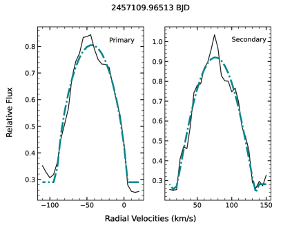
The broadening function (BF) is a representation of spectral profiles in velocity space. The BF contains signatures of the $v_{r}$ shifts of different lines and also intrinsic stellar effects like rotational broadening, spots, pulsations, etc. (Rucinski, 1999). We calculated the BF for one of the composite spectra of AI Hya to estimate $v\sin i$ values for the primary and secondary components, respectively. This process serves to remove the degeneracy between $v\sin i$ and other atmospheric parameters like $T\mathrm{{}_{eff}}$ and [M/H]. A modified version of the treatment described in Rucinski (1999) was adopted and a multi Gaussian fit was implemented. The BF was calculated in a wavelength range of 4080-5000 Å. A synthetic solar-type spectrum with zero projected rotational velocity $v\sin i$ was used as our template. To deal with the noise in the data, a Gaussian smoother of 3 $\mathrm{km\,s^{-1}}$ rolling window was applied to the BF. Two clear peaks were visible in the velocity space, as shown in Figure 6, corresponding to the primary and secondary components. The peaks were fitted with the rotational profile,

$$G(v)=A\left[c_{1}\sqrt{1-\left(\frac{v}{v_{max}}\right)^{2}}+c_{2}\left(1-\left(\frac{v}{v_{max}}\right)^{2}\right)\right]+lv+k$$ (1)

where $A$ is the area under the profile, $v_{max}$ is the maximum velocity shift which occurs at the equator (Gray, 2005), $c_{1}$ and $c_{2}$ are constants which are a function of limb darkening themselves, while $l$ and $k$ are correction factors to the BF continuum. The BF fit was calculated for the spectra with the highest SNR and good separation between the components in velocity space. The best BF fit to the line profile of the primary and secondary binary components are shown in Fig.6. Fixing the obtained values of $v\sin i$ from this analysis and $\log g$ from the light curve solution, the gssp_composite fitting routine was applied to obtain stellar temperatures $T_{\rm eff}$_(1,2), microturbulent velocities $\xi$ and global metallicities [M/H].

Figure 6: Broadening functions for the primary and secondary components of AI Hydrae calculated using HIDES spectra (epoch: 2457109.96513 HJD), which provided a good SNR and velocity separation between the two components. The blue, dashed line represents best-fit rotational function (Group-P).

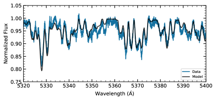
The step size of the grid gives us a rough idea of the errors involved. However, to obtain more robust error estimates we plotted the $\chi^{2}$ data for each parameter and fitted a parabola to obtain the minimum; its distance to the intercepts on the abscissa are taken as the errors. These parameters are obtained for a total of four spectra and then averaged out. The remaining spectra were not suitable for the analysis in gssp due to lower SNR. The results of the analysis are compiled in Table 3 and a sample of the fit to one of the spectra is shown in Figure 7.

Figure 7: A snippet of the best-fit model generated by gssp for the given set of parameters (Group-P).

4.2.2 iSpec

A complimentary spectroscopic analysis was performed on the disentangled spectra of the primary and secondary stars using iSpec (Blanco-Cuaresma et al., 2014). Before the analysis, the spectra are treated for $v_{r}$ offset and continuum correction. Estimates of flux errors were introduced as a sum of errors calculated from SNR, and flux-scaled residuals from the disentangled routine. For the spectroscopic analysis we fixed the $\log g$  parameter with values obtained from the light curve solution and limb darkening parameters with values adopted from Claret & Bloemen (2011).

We fit the model using the spectral synthesis approach. This is done by implementing the use of the spectrum code (Gray & Corbally, 1994), a marcs (Gustafsson et al., 2008) grid of model atmospheres, and solar abundances taken from Asplund et al. (2009). We adopt a two-step process. The initial run is aimed at estimating the global metallicity ([M/H]) by keeping it as a free parameter. The macroturbulent velocity (v_mac) and alpha enhancement parameters were set to zero as v_mac has a negligible contribution for stars in the concerned temperature range and alpha enhancement, when set as a free parameter, produced implausible values. $v\sin i$ was set to the values obtained by the BF analysis. We compared the obtained value for [M/H] with results from the gssp analysis and found it to be consistent with the errors. The average value of [M/H] was calculated and fixed for the next step where we fit for temperature $T_{\rm eff}$, microturbulent velocity $\xi$, and abundances of Iron (Fe), Nickel (Ni) and Chromium (Cr), as these were the prominent lines in the chosen spectral range.

The output parameters obtained from iSpec are given in Table 3 and Table 4. It is to be noted that Fe, Ni, and Cr are more abundant in the primary compared to solar values and those of the secondary star. This trend in the abundances is in agreement with the values obtained by group-K. The output parameters for the secondary star agree fairly well with those from the gssp analysis and from the group-K. The best fit solution for the primary component, as in the case of gssp analysis, also hinted towards a lower $T_{\mathrm{eff}}$ compared to the group-K solution.

5 Binary modelling

5.1 Group-K

To update the fundamental stellar parameters ($M$, $R$) of AI Hya, we performed binary modelling with the help of the determined atmospheric parameters and the results of the $v_{r}$  investigation.

In binary modelling, the TESS data were used. However, the shapes of the eclipses of AI Hya are distorted due to the pulsations. Thus we first cleaned the pulsations and only then carried out the binary modelling. Therefore, the Period04 program (Lenz & Breger, 2005) was used to detect the variations caused by oscillations. The derived pulsation frequencies were cleaned from the light curve and the residuals were used in the binary modelling.

In this analysis, we used the Wilson-Devinney code (Wilson & Devinney, 1971) combined with Monte-Carlo simulations (Zola et al., 2004, 2010). The pulsation removed data were binned to around 4000 points to be used in the binary modelling code. AI Hya is classified as a detached binary system in the literature (Lee, Hong, & Kristiansen, 2020). According to their results (e.g., for $\Omega$, $q$, $a$), both components do not seem to fill their Roche lobe, hence the system is defined as a detached binary. Also, the morphology of the light curve, i.e. very small ellipsoidal variations and eclipses spanning a small fraction of the orbital period, confirm this classification. Therefore, a detached binary configuration was considered our analysis. In the modelling, we took some parameters fixed, such as the $T_{\rm eff}$  of the hotter component, $P_{\rm orb}$, $q$ taken from our results and bolometric albedos (Ruciński, 1969), bolometric gravity-darkening coefficient (von Zeipel, 1924), and the logarithmic limb darkening coefficient (van Hamme, 1993) taken the same as given Kahraman Aliçavuş & Aliçavuş (2019). The orbital inclination ($i$), $T_{\rm eff}$  of the cooler component, phase shift ($\phi$), $e$, $a$, $\omega$, and dimensionless potential ($\Omega$) of the components were set free.

Table 5: Results of the light curve analysis and the fundamental stellar parameters. The Subscripts 1, 2 and 3 represent the hotter, the cooler, and third binary components, respectively. ^a Shows the Fixed Parameters.

Parameter	Value	Value
	Group-K	Group-P
$i$ (o)	89.866 $\pm$ 0.015	89.837 $\pm$ 0.136
$T$1a (K)	7700 $\pm$ 100	7330 $\pm$ 170
$T$2 (K)	7180 $\pm$ 230	7210 $\pm$ 150
$\Omega$1	11.412 $\pm$ 0.046	-
$\Omega$2	8.961 $\pm$ 0.035	-
Phase shift	-0.0310 $\pm$ 0.0001	-
$q$	1.074a	1.075
$r$1∗ (mean)	0.1001 $\pm$ 0.0036	0.1015 $\pm$ 0.0005
$r$2∗ (mean)	0.1412 $\pm$ 0.0026	0.1412 $\pm$ 0.0006
$l$1 / ($l$1+$l$2)	0.381 $\pm$ 0.016	0.374 $\pm$0.02
$l$2 / ($l$1+$l$2)	0.619 $\pm$ 0.016	0.616 $\pm$ 0.02
$l$3	0.0	0.0
Derived Quantities
$M$1 ($M_{\odot}$)	1.950 $\pm$ 0.033	1.950 $\pm$ 0.033
$M$2 ($M_{\odot}$)	2.096 $\pm$ 0.035	2.096 $\pm$ 0.035
$R$1 ($R_{\odot}$)	2.754 $\pm$ 0.015	2.787 $\pm$ 0.020
$R$2 ($R_{\odot}$)	3.863 $\pm$ 0.021	3.877 $\pm$ 0.026
log ($L$1/$L_{\odot}$)	1.381 $\pm$ 0.034	1.311 $\pm$ 0.081
log ($L$2/$L_{\odot}$)	1.554 $\pm$ 0.035	1.549 $\pm$ 0.097
$\log g$1 (cgs)	3.848 $\pm$ 0.003	3.838 $\pm$ 0.005
$\log g$2 (cgs)	3.586 $\pm$ 0.003	3.582 $\pm$ 0.005
$M_{bol}$1 (mag)	1.30 $\pm$ 0.08	1.474 $\pm$ 0.202
$M_{bol}$2 (mag)	0.87 $\pm$ 0.08	0.877 $\pm$ 0.243
$M_{V}$1 (mag)	1.25 $\pm$ 0.08	1.424 $\pm$ 0.208
$M_{V}$2 (mag)	0.79 $\pm$ 0.08	0.822 $\pm$ 0.258
Distance (pc)	659 $\pm$ 30	642 $\pm$ 36

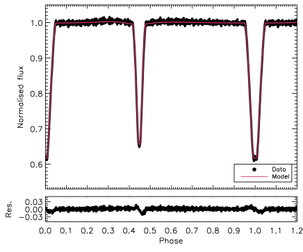
As a result of this analysis, the fundamental parameters of both components of AI Hya were calculated. Additionally, the bolometric ($M_{bol}$) and absolute ($M_{V}$) magnitudes were estimated. The jktabsdim code (Southworth, Maxted, & Smalley, 2004b) and the bolometric correction (Eker et al., 2020) are used in the calculations of these parameters. The outcome of the binary modelling is given in Table 5 and the consistency of the theoretical light curve with the observation is shown in Fig. 8.

When the results of this analysis were examined, one can notice that the more luminous star is the more massive and also the cooler component. This result is consistent with the results found in the $v_{r}$  analysis by group-K.

Figure 8: Theoretical binary modelling fit without spot assumption (solid-line) (Group-K).

5.2 Group-P

Aiming to determine precise physical and orbital parameters of AI Hya, we performed its modelling in version 40 of the jktebop (Southworth, Maxted, & Smalley, 2004b). This program is written by J. Southworth and aimed at modelling light curves of detached eclipsing binaries and is based on the ebop program (Popper & Etzel, 1981). The code treats stars as spheres to calculate the eclipse shapes, and biaxial ellipsoids to calculate proximity effects. The light curves are calculated by numerical integration of concentric circles over each stellar surface. It can deal with stellar oblateness of up to 4% making it a good choice for AI Hya. The photometric data remain the same as used by Group-K.

The parameters set as free are $P_{\rm orb}$, time of minima of the primary eclipse $T_{o}$, inclination $i$, eccentricity $e$, argument of periastron $\omega$, surface brightness ratio $J$ (secondary/primary), ratio of radii ($\frac{\mathrm{r{{}_{A}}}}{\mathrm{r{{}_{B}}}}$), and the sum of radii (r_A+r_B). These radii are relative to the semi-major axis. For the limb darkening coefficients, we use a logarithmic law and set their initial values according to Claret (2017). The coefficients were fixed for the initial fit and were perturbed at the error estimation step.

The code gives an option to include multiple sine and polynomial functions during the light curve modelling to account for periodic and long-term trends. We use this functionality to our advantage to pseudo-model the observed pulsations so that their effect on the binary model is minimal, giving us an improved precision. We analyse the out-of-eclipse portions of the light curve using pyriod, and use the frequencies to initialise the sinusoids in the jktebop input files. This is done in an iterative way where we add one sine with a constant period and fit for its epoch and amplitude. The frequency is kept if the model is improved significantly; otherwise the next most prominent frequency is taken. In this analysis, we used a total of 9 sines, which is the limit for jktebop. The number of independent frequencies of AI Hya is higher than this maximum limit, hence we are left with some residual pulsation signals as seen in Figure 9 and Figure 10.

Figure 9: jktebop model with 9 sines used to model the pulsations (Group-P).

Figure 10: Zoomed-in view of the model over an orbit (Group-P).

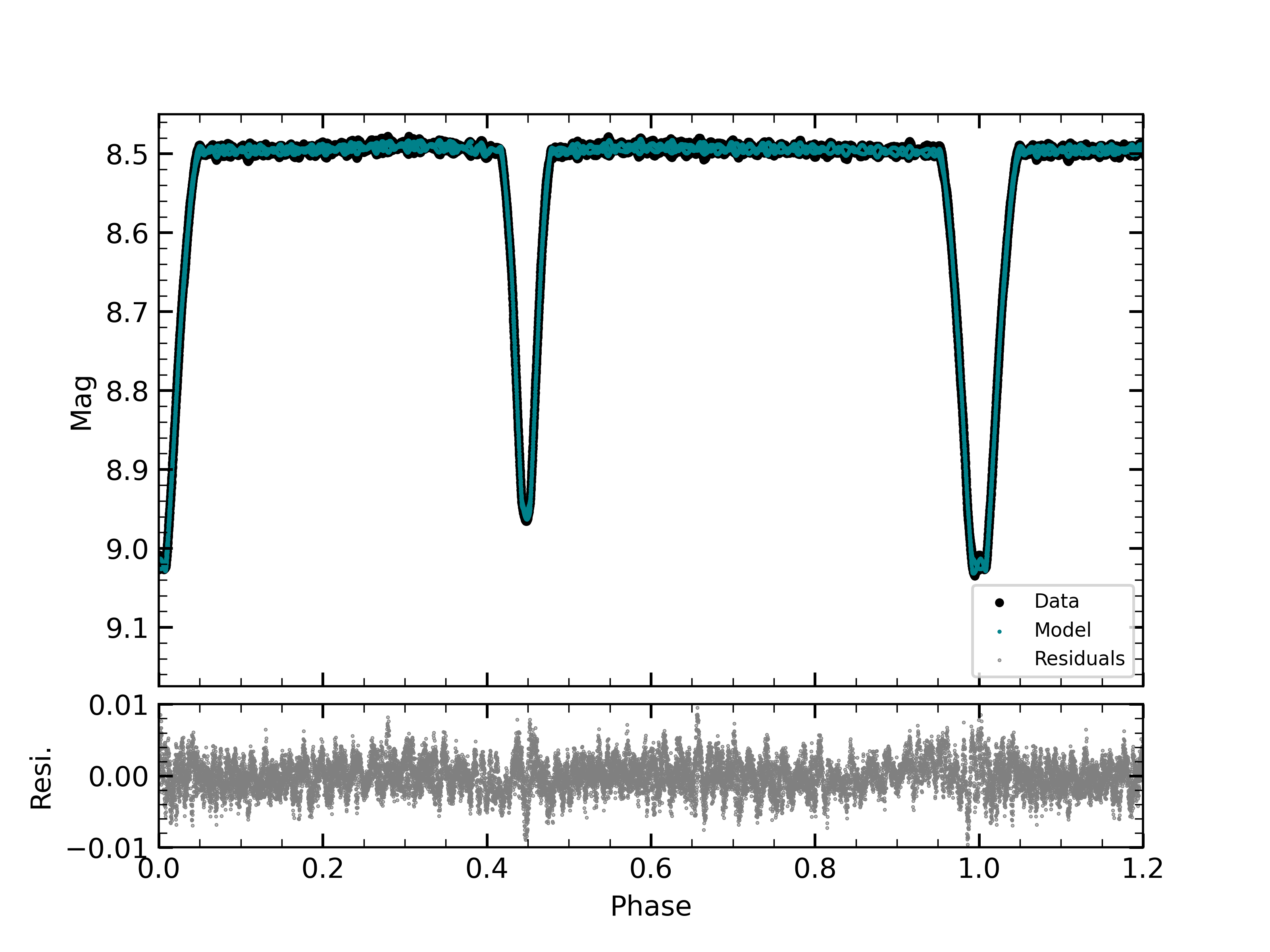
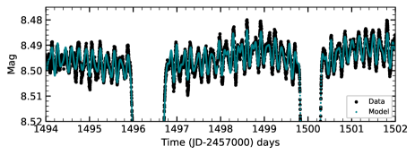
Once the sines are fixed to the best fit values of epoch, period and amplitudes, we make the Monte Carlo runs for error estimation. The results of this analysis are mentioned in Table 5, in comparison to the values obtained by group-K. Similarly to the other group, we used the results of $v_{r}$, and jktebop solutions to calculate a set of absolute parameters, including masses, radii, luminosities, and distance. The effective temperatures mentioned in the table are an average over the sum of $T_{\mathrm{eff}}$ obtained from gssp and iSpec analysis.

6 Frequency analysis of the pulsations

AI Hya was observed by TESS during observation sector 7 in January/February 2019. We used the Simple Aperture Photometry data from the 2-min cadence light curves available at the Mikulski Archive for Space Telescopes (MAST). This time series spans 24.45 d and contains 16362 measurements. To determine the pulsation frequencies, we used only the data that were taken out of eclipse, which reduced the data set to 14019 measurements (time span 24.07 d).

This time series was analysed using the Period04 software (Lenz & Breger, 2005) by group-K. This package applies single-frequency power spectrum analysis and simultaneous multi-frequency sine-wave fitting. These sine-wave fits are subtracted from the data and the residuals examined for the presence of further periodicities. The application of this procedure to AI Hya is illustrated in Fig. 11.

Figure 11: The Fourier Transform of the out-of-eclipse TESS light curve of AI Hya (top) and subsequent prewhitening steps. The blue arrows denote the signals detected. Outside of the frequency range shown no significant signal is present.

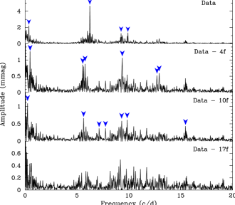
During such a process, it is important to decide where to stop. Often this is facilitated via the application of SNR criteria. In this work, we have adopted the strategy proposed by Breger et al. (1993) which is to compute the ratio of the signal amplitude relative to the local noise level to determine whether the frequency under consideration represents a significant detection. Whereas Breger et al. (1993) propose SNR $>$ 4 for a detection, recent findings for space-based data (e.g., Baran & Koen, 2021) suggest that a more conservative limit must be chosen. Given the restricted frequency range in which we search for periodicities, our requirement was SNR $>$ 4.5. Furthermore, in unresolved frequency spectra, the periodic content present in the time series can easily be overinterpreted (Balona, 2014) which suggests caution regarding the present data set. Consequently, we stopped the frequency search after the detection of 17 signals (lowest panel of Fig. 11). More periodicities are certainly present, but these need to await a longer data set for reliable detection. We list the frequency solution so derived in Table 6.

Table 6: A least squares fit of the pulsation frequencies of AI Hya. Formal error estimates for the independent frequencies and phases (Montgomery & O’Donoghue, 1999) are given in braces in units of the last digits after the comma.

	Frequency	Amplitude	SNR
	d-1	mmag
		$\pm 0.02$
$\nu_{1}$	6.2412(1)	4.75	54.2
$\nu_{2}$	9.2654(4)	1.18	9.7
$\nu_{3}$	9.9065(4)	1.20	9.4
$\nu_{4}$	12.715(1)	0.48	4.5
$\nu_{5}$	12.928(1)	0.54	5.4
$\nu_{6}$	9.3689(4)	1.42	11.5
3$\nu_{orb}$	0.3619	1.76	7.5
4$\nu_{orb}$	0.4825	1.32	5.9
$\nu_{7}$	5.5599(7)	0.78	8.3
$\nu_{8}$	5.7804(1)	0.69	7.5
2$\nu_{orb}$	0.2413	1.75	7.3
$\nu_{9}$	5.6375(7)	0.73	7.7
$\nu_{10}$	7.136(1)	0.37	6.0
$\nu_{11}$	7.751(1)	0.39	5.2
$\nu_{12}$	9.3051(6)	0.82	6.7
$\nu_{13}$	9.8432(8)	0.69	5.3
$\nu_{3}+\nu_{7}$	15.464(1)	0.43	5.6

This table also contains three harmonics of the orbital period. These are not pulsation frequencies, but a consequence of residual binary-induced variability (see Section on binary modeling for a discussion). The pulsation frequencies themselves were found in an interval between 5.5 – 13.0 d^-1, with one possible combination frequency. It is however not clear whether this is a real combination or just a numerical coincidence keeping in mind the short data set, hence poor frequency resolution. Our frequency solution is similar to that reported by Lee, Hong, & Kristiansen (2020) apart from their identification of possible combination frequencies that are partly implausible.

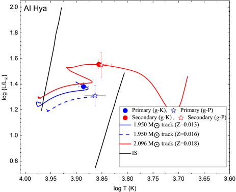
To use the pulsations to learn more about the individual components by applying asteroseismic methods, it is essential to know from which star the pulsations originate. A quick look at the TESS light curve reveals that pulsations are clearly visible during the total part of the primary eclipse, meaning that the secondary is the source of the highest amplitude oscillations. However, both components of AI Hya are located within the pulsational instability strip of the $\delta$ Scuti stars (Murphy et al., 2019, see Fig. 12), thus the primary may pulsate as well. $\delta$ Scuti stars generally pulsate in pressure and mixed modes of low radial order (e.g., Breger, 2000). Using the stellar parameters from Table 5, we can compute the expected frequency of the radial fundamental mode of both pulsators from the pulsation constant $Q=P\sqrt{\rho/\rho_{\odot}}=PM^{1/2}R^{-3/2}$, assuming $Q$ to be 0.033 d for this mode (Fitch, 1981). We thus expect the radial fundamental mode frequency of the primary component to be around 9.3 d^-1, and around 5.8 d^-1 for the secondary component, respectively. In Table 6 oscillation frequencies around both these values are seen, which allows no more than the educated guess that the pulsations below $\sim 8$ d^-1 would arise from the secondary component, whereas the higher frequency modes could originate from either star.

A determination of the origin of the pulsations from the orbital light time effect is unfortunately out of reach. The expected light time effect would be about 30 s (cf. Table 2). An attempt to measure the effect for the strongest pulsation frequency yielded $35\pm 111$ s, a null result. To conclude, because it is impossible to say with confidence which pulsation frequencies arise from which component of AI Hya, an asteroseismic analysis cannot be carried out.

7 Evolutionary models

The evolutionary status of the binary components was examined by utilizing the Modules for Experiments in Stellar Astrophysics (mesa) evolution code (Paxton et al., 2011, 2013) which includes a binary module (Paxton et al., 2015) to examine the binary orbital evolution and to determine the initial parameters of binary systems. In this examination, various evolutionary models were generated considering different metallicity ($Z$). In the models, MESA equation-of-state (EOS) were used. The EOS tables are based on the OPAL EOS tables (Rogers & Nayfonov, 2002). The OPAL opacity tables and the default solar mixtures were adopted as Z initial fraction from Asplund et al. (2009). Helium mass fraction were taken Y=0.28, for Z=0.02. Convective core overshoot was described by the exponentially decaying prescription of Herwig (2000) and overshooting parameter adopted 0.20 for both components (Claret & Torres (2016) find 0.208 for both components). A mixing length $\alpha_{MLT}$  value of 1.8 was used as the theoretical $\delta$ Scuti  instability strip (Dupret et al., 2004, 2005) was obtained with this $\alpha_{MLT}$ value.

Taking into account the calculated parameters in the binary modelling for both groups, the evolutionary status of the binary components was investigated. As a result, we found that the secondary (more luminous) binary component can be represented with the same evolutionary tracks according to both groups’ results. However, the less luminous primary component’s position was determined with different $Z$ parameters as the parameters of this star were found to be slightly different in the study of the two groups. According to the evolutionary models, the $Z$ parameters of both binary components were found similar to solar (Asplund et al., 2009) within the errors which differs from the results of the groups as we determined that the less luminous component’s atmosphere is somewhat enhanced in metals. The results of this analysis are given in Table 7 and a H-R diagram is shown in Fig. 12. The observational borders of the $\delta$ Scuti  instability strip were taken from Murphy et al. (2019). As can be seen from the H-R diagram, both binary components are placed inside the $\delta$ Scuti  instability strip.

8 Discussion and Conclusions

In this analysis, we present the results of the detailed analysis of AI Hya carried out by two independent groups. The system was observed with different high-resolution spectrographs (R$\gtrsim$38000). The radial velocity variations of AI Hya were modelled using the $v_{r}$  measurements of both groups and the orbital parameters such as $T_{0}$, $P_{\rm orb}$, $e$ and $q$ were updated. The resulting parameters of the analysis of both groups are consistent with each other within the errors and they slightly differ from the results of Popper (1988). Especially the $e$ value shows a discrepancy. Popper (1988) found $e$ to be 0.2301 $\pm$ 0.0015 while in our study it was determined as 0.2419 $\pm$ 0.0036 and 0.2432 $\pm$ 0.0050 by group-P and -K, respectively.

Since our high-resolution spectra are spread over all orbital phases, we were able to derive the atmospheric parameters of both binary components by modelling either the composite spectra or the spectra of the individual components after applying spectral disentangling. To derive the atmospheric parameters, $v\sin i$  and the chemical composition of the binary components, group-K analysed disentangled spectra of the components, while group-P performed their analysis using both the composite and disentangled spectra. As a result, group-K found that the more luminous star is cooler than the less luminous component. They found the $T_{\rm eff}$  values from the $H_{\beta}$ line fit and Fe lines to be 7500 $\pm$ 200 K and 7700 $\pm$ 100 K for the primary and 7000 $\pm$ 150 K and 7200 $\pm$ 100 K for the secondary component, respectively. Group-P used two different codes in their analysis. With the gssp code analysis they found a similar result with group-K even though the resulting $T_{\rm eff}$  values differ from each other, they determined that the more luminous star is cooler (7150 $\pm$ 250 K) and less luminous one is hotter (7350 $\pm$ 300 K). In the iSpec analysis of group-P, $T_{\rm eff}$  values of both components were found similar to the results of the gssp analysis within error bars. The primary’s temperature is the most significant discrepancy between the values derived by the two groups. The exact reason for this temperature inconsistency is not fully understood, although it is still only at a level of $\sim$1.1$\sigma$.

In the chemical abundance analysis, both groups found the less luminous but hotter binary component to show overabundance while the other component has chemical abundance similar to solar. Both groups determined the abundances of some individual elements such as iron (Fe). They derived Fe abundances as 8.25 $\pm$ 0.23 (group-K) and 7.83 $\pm$ 0.16 (group-P). These values are consistent with each other within their 1$\sigma$ errors, and both demonstrate that the hotter component has a slightly metal-rich chemical abundance compared to solar values (see Table 4). This comes somewhat to a surprise, as this binary system should have been formed in the same interstellar environment and hence its components should have the same chemical composition. The difference could be due to the consequences of the evolution of the system. If AI Hya had a very eccentric orbit when the system was formed, there could be some material flows from one component to another that could have changed the diffusion in one component. Another explanation was given by Yushchenko et al. (2015) and they pointed out that possible gas and dust accretion from the circumstellar envelope could alter the atmospheric composition of one component.

After the determination of the atmospheric parameters, they were used as input in the binary modelling. Overall, even though both working groups used different approaches to estimate the parameters of the binary component of AI Hya, the values determined by both groups are found to be consistent with each other within the error bars. The two groups obtained very similar $M$ and $R$ values with a $\leq$1.7% and $\sim$0.5% accuracy, respectively. When we compare these values with the ones found by Lee, Hong, & Kristiansen (2020), we notice that there are slight differences, especially in the $R$ parameters, and there is significant diversity in the calculated distance. These differences could be caused by the different assumptions of the atmospheric parameters.

The evolutionary status of the system was examined and it was found that both binary components are inside the $\delta$ Scuti  instability strip. The age of the system is determined as well. According to the determined ages, we could say that AI Hya is in an important evolutionary phase in terms of binary evolution. The rapidly evolving massive component will begin the mass transfer process to the less massive one approximately 20 Myr from now. This situation could cause significant variations in the oscillation properties. Increasing the number of such bodies is important in terms of examining the pulsating structures before the mass transfer processes.

Table 7: Results obtained from the best-fit evolutionary models.

Parameter	Group-K	Group-P
$P$initial (days)	8.34 (1)	8.34 (1)
$e$initial	0.242 (2)	0.243 (2)
$Z$1	0.013 (2)	0.016 (2)
$Z$2	0.018 (2)	0.018 (2)
Age (Myr)	850 (20)	860 (20)

The pulsation properties of AI Hya were examined using the TESS data. However, the system has only one sector of SC data, which offers us a poor frequency resolution. In the analysis, pulsation frequencies were found between 5.5 and 13 d^-1. As both binary components are placed in the $\delta$ Scuti instability strip, we were unable to say whether one or both pulsate. Apart from that, we could not find pulsations related to the orbital frequency.

As a result of this study, we thoroughly examined a detached binary system showing oscillations. This kind of objects is particularly important to examine the instability strip of $\delta$ Scuti stars since they allow us to determine fundamental astrophysical, atmospheric parameters and the chemical abundances of individual binary components. Hence an increasing number of analyses of such systems is expected to be essential to deeply understand the nature of pulsations.

Figure 12: The positions of the binary components in the H-R diagram according the results of both group-K (g-K) and group-P (g-P). The instability strip (IS) borders of the $\delta$ Scuti  stars were taken from Murphy et al. (2019).

DATA AVAILABILITY

The data underlying this work will be shared at reasonable request to the corresponding author.

Table A1: The $v_{r}$ measurements. The subscripts “1” and “2” represent the more and the less luminous components, respectively.

HJD	$v_{r,1}$	$v_{r,2}$	Instrument
+2450000	(km s-1)	(km s-1)
9263.45270	-12.6 $\pm$ 2.8	109.3 $\pm$ 2.7	CAOS
9161.65803	132.8 $\pm$ 1.8	-48.3 $\pm$ 1.7	HERMES
9162.64306	109.8 $\pm$ 2.0	-21.7 $\pm$ 1.5	HERMES
9230.65226	121.5 $\pm$ 1.6	-24.7 $\pm$ 1.8	HERMES
9231.66393	124.1 $\pm$ 1.7	-24.9 $\pm$ 1.7	HERMES
9233.62648	59.8 $\pm$ 5.7	36.1 $\pm$ 3.4	HERMES
9234.55784	20.6 $\pm$ 2.1	72.1 $\pm$ 2.5	HERMES
9237.61273	15.0 $\pm$ 1.6	77.3 $\pm$ 1.5	HERMES
9235.43315	-46.3 $\pm$ 1.5	130.3 $\pm$ 1.8	HERMES
9257.49195	98.8 $\pm$ 1.8	-2.9 $\pm$ 2.0	HERMES
9260.61123	-33.9 $\pm$ 1.7	117.9 $\pm$ 1.9	HERMES
9276.55613	96.6 $\pm$ 2.0	-8.4 $\pm$ 1.2	HERMES
9296.42427	88.7 $\pm$ 1.7	-3.8 $\pm$ 2.0	HERMES
9297.44747	126.7 $\pm$ 1.8	-37.4 $\pm$ 2.2	HERMES
9298.45846	113.5 $\pm$ 1.7	-16.0 $\pm$ 1.8	HERMES
9299.46357	78.1 $\pm$ 2.1	12.5 $\pm$ 2.3	HERMES
7075.62231	-39.7 $\pm$ 1.5	129.9 $\pm$ 0.5	CORALIE
7076.63954	-20.4 $\pm$ 1.2	120.0 $\pm$ 1.3	CORALIE
7109.63123	-17.9 $\pm$ 2.4	126.0 $\pm$ 1.3	CORALIE
7022.31643	118.5 $\pm$ 1.9	-31.4 $\pm$ 0.5	HIDES
7060.09414	-13.6 $\pm$ 0.7	118.2 $\pm$ 0.6	HIDES
7109.96513	-18.6 $\pm$ 1.1	114.6 $\pm$ 0.6	HIDES
7114.92732	120.1 $\pm$ 1.2	-34.0 $\pm$ 0.7	HIDES
7146.98403	118.5 $\pm$ 1.3	-42.9 $\pm$ 0.8	HIDES
7147.96084	131.3 $\pm$ 1.2	-42.3 $\pm$ 0.6	HIDES
7363.28986	135.7 $\pm$ 0.6	-48.4 $\pm$ 0.7	HIDES
7755.22744	-34.0 $\pm$ 0.7	126.5 $\pm$ 0.7	HIDES
7813.13416	-25.2 $\pm$ 0.8	124.3 $\pm$ 0.9	HIDES
7814.08321	-28.3 $\pm$ 0.9	126.6 $\pm$ 0.9	HIDES
7846.01822	-10.8 $\pm$ 1.7	113.4 $\pm$ 1.0	HIDES
8035.34461	101.6 $\pm$ 0.7	-13.9 $\pm$ 0.8	HIDES
8066.24908	85.2 $\pm$ 0.8	-4.1 $\pm$ 1.3	HIDES

References

- Aerts, Christensen-Dalsgaard, & Kurtz (2010) Aerts C., Christensen-Dalsgaard J., Kurtz D. W., 2010, aste.book
- Antoci et al. (2014) Antoci V., Cunha M., Houdek G., Kjeldsen H., Trampedach R., Handler G., Lüftinger T., et al., 2014, ApJ, 796, 118. doi:10.1088/0004-637X/796/2/118
- Asplund et al. (2009) Asplund M., Grevesse N., Sauval A. J., Scott P., 2009, ARA&A, 47, 481
- Balona (2014) Balona L. A., 2014, MNRAS, 439, 3453
- Baran & Koen (2021) Baran, A. S. & Koen, C., 2021, AcA, 71, 113
- Blanco-Cuaresma et al. (2014) Blanco-Cuaresma S., Soubiran C., Heiter U., Jofré P., 2014, A&A, 569, A111. doi:10.1051/0004-6361/201423945
- Borucki et al. (2010) Borucki W. J., Koch D., Basri G., Batalha N., Brown T., Caldwell D., Caldwell J., et al., 2010, Sci, 327, 977. doi:10.1126/science.1185402
- Bowman & Kurtz (2018) Bowman D. M., Kurtz D. W., 2018, MNRAS, 476, 3169. doi:10.1093/mnras/sty449
- Breger (2000) Breger, M., 2000, in Delta Scuti and Related Stars, ed. M. Breger & M. H. Montgomery, ASP Conf. Ser. 210, 3
- Breger et al. (1993) Breger, M., et al., 1993, A&A, 271, 482
- Catanzaro, Leone, & Dall (2004) Catanzaro G., Leone F., Dall T. H., 2004, A&A, 425, 641
- Catanzaro et al. (2022) Catanzaro G., Colombo C., Ferrara C., Giarrusso M., 2022, MNRAS, 515, 4350. doi:10.1093/mnras/stac1723
- Catanzaro et al. (2019) Catanzaro G., Busà I., Gangi M., Giarrusso M., Leone F., Munari M., 2019, MNRAS, 484, 2530. doi:10.1093/mnras/stz080
- Claret (2017) Claret A., 2017, A&A, 600, A30. doi:10.1051/0004-6361/201629705
- Claret & Torres (2016) Claret A., Torres G., 2016, A&A, 592, A15. doi:10.1051/0004-6361/201628779
- Coelho et al. (2005) Coelho P., Barbuy B., Meléndez J., Schiavon R. P., Castilho B. V., 2005, A&A, 443, 735. doi:10.1051/0004-6361:20053511
- Dupret et al. (2004) Dupret M.-A., Grigahcène A., Garrido R., Gabriel M., Scuflaire R., 2004, A&A, 414, L17
- Dupret et al. (2005) Dupret M.-A., Grigahcène A., Garrido R., Gabriel M., Scuflaire R., 2005, A&A, 435, 927. doi:10.1051/0004-6361:20041817
- Eker et al. (2020) Eker Z., Soydugan F., Bilir S., Bakış V., Aliçavuş F., Özer S., Aslan G., et al., 2020, MNRAS, 496, 3887. doi:10.1093/mnras/staa1659
- Fitch (1981) Fitch, W. S., 1981, ApJ 249, 218
- Gaia Collaboration (2022) Gaia Collaboration, 2022, Gaia DR3: data release content and main properties. A&A, in prep.
- Gaulme & Guzik (2019) Gaulme P., Guzik J. A., 2019, A&A, 630, A106. doi:10.1051/0004-6361/201935821
- Gray & Corbally (1994) Gray R. O., Corbally C. J., 1994, AJ, 107, 742. doi:10.1086/116893
- Gustafsson et al. (2008) Gustafsson B., Edvardsson B., Eriksson K., Jørgensen U. G., Nordlund Å., Plez B., 2008, A&A, 486, 951. doi:10.1051/0004-6361:200809724
- Grevesse, Asplund, & Sauval (2007) Grevesse N., Asplund M., Sauval A. J., 2007, SSRv, 130, 105. doi:10.1007/s11214-007-9173-7
- Iglesias-Marzoa et al. (2015) Iglesias-Marzoa, R., López-Morales, M., & Jesús Arévalo Morales, M. 2015, pasp, 127,567
- Handler et al. (2020) Handler G., Kurtz D. W., Rappaport S. A., Saio H., Fuller J., Jones D., Guo Z., et al., 2020, NatAs, 4, 684. doi:10.1038/s41550-020-1035-1
- Herwig (2000) Herwig F., 2000, A&A, 360, 952
- Ilijic et al. (2004) Ilijic S., Hensberge H., Pavlovski K., Freyhammer L. M., 2004, ASPC, 318, 111
- Jayasinghe et al. (2018) Jayasinghe T., et al., 2018, MNRAS, 477, 3145
- Joergensen & Gronbech (1978) Joergensen H. E., Gronbech B., 1978, A&A, 66, 377
- Kahraman Aliçavuş et al. (2016) Kahraman Aliçavuş F., et al., 2016, MNRAS, 458, 2307
- Kahraman Aliçavuş et al. (2017) Kahraman Aliçavuş F., Soydugan E., Smalley B., Kubát J., 2017, MNRAS, 470, 915. doi:10.1093/mnras/stx1241
- Kahraman Aliçavuş & Aliçavuş (2019) Kahraman Aliçavuş F., Aliçavuş F., 2019, MNRAS, 488, 5279. doi:10.1093/mnras/stz2003
- Kahraman Aliçavuş et al. (2022) Kahraman Aliçavuş F., Gümüş D., Kırmızıtaş Ö., Ekinci Ö., Çavuş S., Kaya Y. T., Aliçavuş F., 2022, RAA, 22, 085003. doi:10.1088/1674-4527/ac71a4
- Kambe et al. (2013) Kambe E., et al., 2013, PASJ, 65, 15 ş
- Konacki et al. (2010) Konacki M., Muterspaugh M. W., Kulkarni S. R., Hełminiak K. G., 2010, ApJ, 719, 1293. doi:10.1088/0004-637X/719/2/1293
- Kreiner (2004) Kreiner J. M., 2004, AcA, 54, 207
- Kurtz et al. (2020) Kurtz D. W., Handler G., Rappaport S. A., Saio H., Fuller J., Jacobs T., Schmitt A., et al., 2020, MNRAS, 494, 5118. doi:10.1093/mnras/staa989
- Kurucz & Avrett (1981) Kurucz R. L., Avrett E. H., 1981, SAOSR, 391,
- Kurucz (1993) Kurucz R., 1993, KurCD, 13,
- Lampens (2021) Lampens P., 2021, Galax, 9, 28. doi:10.3390/galaxies9020028
- Lee, Hong, & Kristiansen (2020) Lee J. W., Hong K., Kristiansen M. H., 2020, PASJ, 72, 37. doi:10.1093/pasj/psaa020
- Lenz & Breger (2005) Lenz P., Breger M., 2005, CoAst, 146, 53
- Leone, et al. (2016) Leone F., et al., 2016, AJ, 151, 116
- Liakos & Niarchos (2017) Liakos A., Niarchos P., 2017, MNRAS, 465, 1181. doi:10.1093/mnras/stw2756
- Montgomery & O’Donoghue (1999) Montgomery M. H., O’Donoghue D., 1999, Delta Scuti Star Newsletter 13, 28
- Murphy et al. (2019) Murphy S., Hey D., Van Reeth, T., Bedding T., 2019, MNRAS 485, 2380
- Paxton et al. (2011) Paxton B., Bildsten L., Dotter A., Herwig F., Lesaffre P., Timmes F., 2011, ApJS, 192, 3
- Paxton et al. (2013) Paxton B., et al., 2013, ApJS, 208, 4
- Paxton et al. (2015) Paxton B., et al., 2015, ApJS, 220, 15
- Pepe et al. (2018) Pepe F., Bouchy F., Mayor M., Udry S., 2018, haex.book, 190. doi:10.1007/978-3-319-55333-7_190
- Pilecki et al. (2017) Pilecki B., Gieren W., Smolec R., Pietrzyński G., Thompson I. B., Anderson R. I., Bono G., et al., 2017, ApJ, 842, 110. doi:10.3847/1538-4357/aa6ff7
- Pojmański (2002) Pojmański G., 2002, AcA, 52, 397
- Popper & Etzel (1981) Popper D. M., Etzel P. B., 1981, AJ, 86, 102. doi:10.1086/112862
- Popper (1988) Popper D. M., 1988, AJ, 95, 190. doi:10.1086/114627
- Raskin et al. (2011) Raskin G., et al., 2011, A&A, 526, A69
- Ricker et al. (2014) Ricker G. R., Winn J. N., Vanderspek R., Latham D. W., Bakos G. Á., Bean J. L., Berta-Thompson Z. K., et al., 2014, SPIE, 9143, 914320. doi:10.1117/12.2063489
- Rogers & Nayfonov (2002) Rogers F. J., Nayfonov A., 2002, ApJ, 576, 1064. doi:10.1086/341894
- Ruciński (1969) Ruciński S. M., 1969, AcA, 19, 245
- Smalley et al. (2002) Smalley B., Gardiner R. B., Kupka F., Bessell M. S., 2002, A&A, 395, 601
- Southworth et al. (2004a) Southworth J., Zucker S., Maxted P. F. L., Smalley B., 2004, MNRAS, 355, 986. doi:10.1111/j.1365-2966.2004.08389.x
- Southworth, Maxted, & Smalley (2004b) Southworth J., Maxted P. F. L., Smalley B., 2004, MNRAS, 351, 1277
- Southworth (2013) Southworth J., 2013, A&A, 557, A119. doi:10.1051/0004-6361/201322195
- Southworth (2021) Southworth J., 2021, Univ, 7, 369. doi:10.3390/universe7100369
- Stancliffe et al. (2015) Stancliffe R. J., Fossati L., Passy J.-C., Schneider F. R. N., 2015, A&A, 575, A117. doi:10.1051/0004-6361/201425126
- Stassun et al. (2019) Stassun K. G., Oelkers R. J., Paegert M., Torres G., Pepper J., De Lee N., Collins K., et al., 2019, AJ, 158, 138. doi:10.3847/1538-3881/ab3467
- Shulyak et al. (2004) Shulyak D., Tsymbal V., Ryabchikova T., Stütz C., Weiss W. W., 2004, A&A, 428, 993. doi:10.1051/0004-6361:20034169
- Torres, Andersen, & Giménez (2010) Torres G., Andersen J., Giménez A., 2010, A&ARv, 18, 67. doi:10.1007/s00159-009-0025-1
- Tsymbal (1996) Tsymbal V., 1996, ASPC, 108, 198
- Uytterhoeven et al. (2011) Uytterhoeven K., Moya A., Grigahcène A., Guzik J. A., Gutiérrez-Soto J., Smalley B., Handler G., et al., 2011, A&A, 534, A125. doi:10.1051/0004-6361/201117368
- van Hamme (1993) van Hamme W., 1993, AJ, 106, 2096
- von Zeipel (1924) von Zeipel H., 1924, MNRAS, 84, 665
- Wilson & Devinney (1971) Wilson R. E., Devinney E. J., 1971, ApJ, 166, 605
- Yushchenko et al. (2015) Yushchenko A. V., Gopka V. F., Kang Y.-W., Kim C., Lee B.-C., Yushchenko V. A., Dorokhova T. N., et al., 2015, AJ, 149, 59. doi:10.1088/0004-6256/149/2/59
- Zucker & Mazeh (1994) Zucker S., Mazeh T., 1994, ApJ, 420, 806. doi:10.1086/173605
- Zola et al. (2004) Zola S., et al., 2004, AcA, 54, 299
- Zola et al. (2010) Zola S., Gazeas K., Kreiner J. M., Ogloza W., Siwak M., Koziel-Wierzbowska D., Winiarski M., 2010, MNRAS, 408, 464
- Rucinski (1999) Rucinski S., 1999, ASPC, 185, 82
- Gray (2005) Gray D. F., 2005, oasp.book
- Claret & Bloemen (2011) Claret A., Bloemen S., 2011, A&A, 529, A75. doi:10.1051/0004-6361/201116451
- Rucinski (1999) Rucinski S., 1999, TJPh, 23, 271
- Tkachenko (2015) Tkachenko A., 2015, A&A, 581, A129. doi:10.1051/0004-6361/201526513