Phase Transitions in Particle Physics
Results and Perspectives from Lattice Quantum Chromo-Dynamics

Abstract

Phase transitions in a non-perturbative regime can be studied by ab initio Lattice Field Theory methods. The status and future research directions for LFT investigations of Quantum Chromo-Dynamics under extreme conditions are reviewed, including properties of hadrons and of the hypothesized QCD axion as inferred from QCD topology in different phases. We discuss phase transitions in strong interactions in an extended parameter space, and the possibility of model building for Dark Matter and Electro-Weak Symmetry Breaking. Methodological challenges are addressed as well, including new developments in Artificial Intelligence geared towards the identification of different phases and transitions.

 

TalkWorkshop “Phase Transitions in Particle Physics” Talks

1   Introduction

Gauge theories exist in a variety of different phases. The main focus of this manuscript is Quantum Chromo-Dynamics, QCD, the gauge theory describing strong interactions in elementary particle physics. We will concentrate on an ab initio approach, Lattice Field Theory (LFT), and also report on progress within first principles Functional Approaches to QCD (FAs), as well as Effective Field theories (EFTs). We will describe the results that have been obtained, the current challenges, and the future prospects. This overview of the theoretical state of the art is accompanied by reports on the experimental efforts.

We will consider QCD at finite temperature and/or density, as well as in external magnetic fields. In the space spanned by these parameters, symmetries may be realised in different ways, and the change of symmetry corresponds to phase transitions.

At zero temperature the QCD chiral symmetry is spontaneously broken for massless quarks, with the appearance of composite Goldstone bosons. Further, experimental searches for free quarks have been unsuccessful so far, and the accepted wisdom is that in this regime QCD is confining. The interplay of chiral symmetry and confinement is still poorly understood and is an important subject of current research. When the lightest quarks have non-zero masses, the pseudo-Goldstone becomes massive, with a definite prediction for their dependence on the quark masses.

Temperature induces the restoration of chiral symmetry, with an accompanying liberation of light degrees of freedom, a dramatic phenomenon probed in heavy-ion collision experiments. The analysis of the transitions and their characteristics is at the heart of this paper and is described in section 2.

Equally important is the nature of the exotic phase(s) at the high temperatures probed in experiments: a difficult important task is the connection between lattice results, obtained at equilibrium, and experimental observations from heavy ion collisions with their non-equilibrium dynamics. The role of magnetic fields has been investigated as well. These aspects are discussed in section 3. Dense matter poses specific problems: pairing phenomena have been investigated in a variety of approaches, considering different unbalances, and making also natural a connection with condensed matter. The cold and dense matter is not yet directly accessible with LFT simulations. Here our knowledge comes mostly from functional approaches to QCD and low energy effective theories, with a wealth of interesting and important phenomena. Since in this manuscript, we focus on topics amenable to LFT studies, we will not further pursue these important issues.

The aspects of Strong Interactions outlined so far have experimental and phenomenological relevance. High temperature matter, up to temperatures of about 500 MeV, is created and explored in heavy ion collision experiments. Pushing the temperature at higher values, one reaches regions of cosmological relevance, traversed during the evolution of the primordial Universe. Hypothetically, in this region, the freeze-out of axions occurs: axions are dark matter candidates motivated by a natural extension of QCD, originated by the breaking of an anomalous symmetry. The physics of gravitational waves is an important close-by field. The physics of extremely high matter, beyond experimental capabilities, but still far below the Electroweak Transition, in which the topology of QCD plays a major role, is described in section 6.

From a theoretical point of view, QCD is just one among infinitely many non-Abelian gauge theories with chiral symmetries. By simply changing the parameters of the Lagrangian of Strong Interactions, such as the gauge group, i.e. the number of color charges $N$, the matter field content (including the fermion representation and the number of quark flavors $N_{f}$), the spacetime dimension $D$, …it is possible to investigate different theories and the rich phenomenology they exhibit. Such studies enrich our knowledge and provide helpful inspiration and guidance for devising viable theories beyond the Standard Model. In this manuscript, we will primarily discuss the physics of theories with large $N_{f}$: the increase of the number of flavors triggers the restoration of chiral symmetry, and the chirally symmetric phase at large $N_{f}$ is conformally invariant in the infrared. Composite-Higgs models can be built in a specific region of the phase space, i.e., the one close to the conformal window. In the pre-conformal phase the thermal transition may well be stronger, making these theories potentially interesting also for cosmology. These subjects are discussed in section 5.

Lattice methods require the positivity of the Action for the importance sampling involved. This is achieved by rotating the time to the imaginary axes, thus making the metric Euclidean. Even in this case, the positivity of the Action is violated if a chemical potential introduces an imbalance between baryon and anti-baryons, or if a CP violating $\theta$ term is introduced. All these issues are generically known as sign problem, i.e. the failure of importance sampling due to a complex statistical weight. We will highlight the major challenges and some promising avenues in section 4. Next, we will discuss the application of modern artificial intelligence (AI) techniques to the analysis of phase transitions in section 8. This concerns both the recognition of phase transitions from data samples as well as supporting the importance sampling with machine learning.

Finally, in section 28 we will discuss methods from statistical field theory, which are an essential tool for the analysis of phase transitions. Historically, the main approach to studying the critical and near-critical behavior of a theory has been based on the magnetic equation of state: the starting point is the identification of the order parameter and of the symmetry-breaking pattern at the transition. The key concept is universality and the theoretical framework is that of the renormalization group. Recently, the standard approach has been critically reconsidered, with a deeper analysis of the role of gauge symmetries. In recent years, conformal theories have taken center stage: studies of two-point correlation functions may supplement the analysis of the order parameter, and the conformal bootstrap has led to exciting new developments. We will focus on the very small subset of studies and recent developments that are potentially relevant in the analysis of lattice results on phase transitions, without any pretense to cover all the vast subjects of statistical field theory.

In short summary, in this manuscript, we discuss how the properties of the strong interactions depend on the temperature, on different chemical potentials, on the magnetic field, on the quark masses, and on the number of flavors. The material is organized in several Sections, however, our aim is to see and present it as different angles of the same phase diagram. Hopefully, the knowledge of the physical theory – Quantum Chromo-Dynamics with three families of quarks – , which remains the main focus of these studies, will benefit from this broad view.

We dispense with introductory material (see e.g. [1] for a pedagogical introduction to LFTs and [2, 3] for recent LFT reviews, [4, 5, 6] for recent reviews on functional approaches to QCD), and we concentrate on advanced, state-of-the-art methods and results, as well as on promising novel research paths (without any claim to be exhaustive); occasionally the same studies are mentioned in different sections, when they may be looked at from different points of view.

This paper grew out of the workshop “Phase Transitions in Particle Physics” organized at the GGI in Firenze in Spring 2022. The talks presented there are enlisted and referenced in a dedicated bibliography at the end.

2   Thermal Phase Transitions and Critical Points

2.1   QCD Phase Diagram: Expectations

Thermal phase transitions and critical points are pieces of the QCD phase diagram puzzle. Figure 2.1 with three axes denoting temperature $T$, baryon chemical potential $\mu_{B}$, and mass $m_{u,d}$ of degenerate light up and down quarks represents the conjectured QCD phase diagram, as discussed in [7] and references therein.

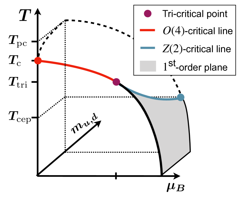
Figure 2.1: Hypothesized phase diagram of QCD assuming a O(4) universality class of the thermal transition in the massless up and down quarks limit, and a physical strange mass. The axes denote the temperature $T$, the baryon-number chemical potential $\mu_{B}$, and the light quark masses $m_{u,d}$. In the front, the situation at zero light quark masses is shown, whereas in the back the phase diagram for physical light quark masses is depicted. A hierarchy of important transition temperatures is indicated as $T_{\mbox{\tiny{pc}}}>T_{\mbox{\tiny{c}}}>T_{\mbox{\tiny{tri}}}>T_{\mbox{\tiny{cep}}}$, with the pseudo-critical transition temperature at physical masses $T_{\mbox{\tiny{pc}}}$, the chiral phase-transition temperature $T_{\mbox{\tiny{c}}}$, the temperature of the tri-critical point $T_{\mbox{\tiny{tri}}}$ and the phase-transition temperature of the critical end-point at physical quark masses $T_{\mbox{\tiny{cep}}}$. Source [7]

In the chiral plane, where $m_{u,d}$ vanishes, for vanishing $\mu_{B}$, restoration of the spontaneously broken $SU(2)_{L}\times SU(2)_{R}$ chiral symmetry group – which is isomorphic to $O(4)$ – as a function of $T$ is expected to be a genuine second order phase transition belonging to $3$-$d$, $O(4)$ universality class occurring at $T_{c}$, which is represented by the red dot in Figure 2.1 . In the region of small baryon chemical potential, phase transition stays second order belonging to $3$-$d$, $O(4)$ universality class; the transition temperature, $T_{c}(\mu_{B})$ decreases with $\mu_{B}$, which is clearly depicted by the bending of red curve originating from $T_{c}(0)$ towards $\mu_{B}$ axis. After $T_{c}(\mu_{B})$ hits the purple tri-critical point at $T_{tri}$ for some value of $\mu_{B}$, the transition becomes first order in the higher $\mu_{B}$ region shown by the black solid line.

Upon adding light quark mass direction to $T$-$\mu_{B}$ plane in the higher $\mu_{B}$ region, for a fixed $m_{u,d}$ value, transition stays first order with decreasing $\mu_{B}$ – this transition would be a line in the grey first order plane starting from the zero $T$ plane – until it reaches a certain combination of $T$, $\mu_{B}$ such that it hits a point on the blue $Z(2)$ critical line and becomes second order belonging to $3$-$d$, $Z(2)$ universality class.

Due to the explicit breaking of the chiral symmetry, the transition is no longer a genuine phase transition for non-zero $m_{u,d}$ but a crossover depicted by the black dashed line. Notice that at the physical value of the light quark masses – the backward plane of the shown QCD phase diagram – and vanishing baryon chemical potential, the crossover transition occurs at a pseudo-critical temperature, $T_{pc}$. This pseudo-critical temperature for the physical value of $m_{u,d}$ decreases as a function of $\mu_{B}$, and the transition remains a crossover until it meets the blue $Z(2)$ critical line at the temperature $T_{\operatorname{\mathrm{cep}}}$ and chemical potential $\mu_{\operatorname{\mathrm{cep}}}$, depicted with the blue dot. The existence of this critical endpoint and its location, $(T_{\operatorname{\mathrm{cep}}}$, $\mu_{\operatorname{\mathrm{cep}}})$, is the modern-day Holy Grail of the experimental as well as the theoretical physics community working on QCD phase diagram and is further discussed in Section 5.

2.2   Degree of Understanding

2.2.1   Lower Density Region

One of the ways to understand the phase diagram of QCD is by employing numerical simulations in the framework of Lattice QCD. In recent years, different lattice studies exploiting chiral observables and their universal scaling features have converged on the value of crossover temperature, $T_{\mathrm{pc}}$ at around $\mathrm{156.5}$ MeV at vanishing $\mu_{B}$ [8, 9]. The value of $T_{c}$ has been found to be equal to $\mathrm{132^{+3}_{-6}}$ MeV, and the same study argues that the phase transition indeed belongs to $3$-$d$, $O(4)$ universality class [10]. Results with Wilson fermions find a compatible value for $T_{c}$ and explore the limits of the $O(4)$ scaling window [11, 12].

Reference [8] is a very accurate study of the curvature of the crossover line in terms of $T_{\mathrm{pc}}$ as a function of $\mu_{B}$ using Taylor expansion around $\mu_{B}=0$, which further boosts confidence in the expected phase diagram picture in the lower density region. We will return to the discussion of the curvature of the crossover line in the next Section.

It is very important to understand the fate of U${}_{\mathrm{A}}(1)$ anomaly at the chiral phase transition of $(2+1)$-flavor QCD – two degenerate light quarks and physical strange quark – [13, 14, 15], Lahiri_talk. Model studies can reveal the interplay of the dynamics of spontaneous and anomalous chiral symmetry breaking, see e.g. [16, 17, 18, 19]. In the scenario where U${}_{\mathrm{A}}(1)$ gets effectively restored near $T_{c}$, references [13, 14, 15] based on one-loop calculation within perturbative $\epsilon$ expansion predict a first-order chiral phase transition for $(2+1)$-flavor QCD, whereas Reference [17] upon employing two different $3$-$d$ perturbative schemes: massive zero-momentum (MZM) scheme and the 3D minimal subtraction scheme MS without $\epsilon$ expansion converges to the possible existence of a stable fixed point. However, the chiral phase transition can only be continuous belonging to O$(4)\times$ O$(2)$ universality class if the considered model lies within the attractive domain of the stable fixed point – in other words, the possibility of a first-order transition is not excluded. The issue can only be settled within full QCD as the strength of anomalous chiral symmetry breaking and its dynamics is related to QCD topology or rather the topological density. This calls for lattice QCD simulations or investigations in functional approaches to QCD, and more references and discussions will be given in Section 6. From the viewpoint of this section, we note that the lattice calculations in the chiral and continuum limit of $(2+1)$-flavor QCD find that the U${}_{\mathrm{A}}(1)$ remains broken at $T_{c}$, and therefore further support the second-order nature of the $(2+1)$-flavor chiral phase transition belonging to $3$-$d$, O$(4)$ universality class [20, 21].

Hadronic correlators provide an important complement to the analysis based on the chiral order parameter, and pole, as well as screening masses, are actively investigated [22, 23, 24]Harris_talk. Hadronic correlators in Euclidean time also serve as input to spectral functions - further discussion can be found in Section 4.

Interestingly, an approximate SU$(4)$ chiral spin-flavour symmetry was recently observed in multiplet patterns of QCD mesonic correlation functions [25, 26]. This symmetry disappears at a temperature of about $300$ MeV, approximatively matching other fast crossovers [27, 12] in the medium which have not yet been completely understood.

Further interesting aspects concern “energy-like" observables which include purely gluonic observables like the Polyakov loop, commonly used as an indicator of confinement/deconfinement crossover for dynamical quarks, as well as heavy quark potential [28] Lahiri_talk,Kudrov_talk. Analysis of flux tubes plays an important role as well [29] in this context. Recent studies addressed the sensitivity of these purely gluonic observables to the chiral phase transition [30].

2.2.2   Scaling Window

The standard picture of critical behavior entails a crossover between genuine critical behavior and a mean-field region. The extent of the scaling window is in general regulated by the Ginzburg criterion, and is non-universal, hence it needs to be settled by numerical simulations. From a phenomenological viewpoint, the scaling window is the region where there is still a memory of the underlying critical behavior. This issue has been studied with functional approaches to QCD as well as in low energy EFTs (Pawlowski_talk, and references therein). EFT studies with O(4)-models and the quark-meson model in [31, 32], for a review see [33], suggest a small critical window with O$(4)$-scaling. Typically, these models assume maximal axial $U(1)$-breaking and the approximations used support O$(4)$ scaling. It has been also argued in these works, that the regime of apparent scaling may be far larger, the difference being hard to extract if the statistical error of the results is sizable. The investigations utilized the functional renormalization group (fRG) that allows direct access to critical scaling. In these models, genuine O(4) scaling was only observed very close to the chiral limit, and it is lost for pion masses $m_{\pi}\gtrsim 1-10$ MeV. These findings were corroborated within functional QCD studies in [34, 35], but a conclusive analysis has not been done yet. The role of the light up and down quark masses, and the extent of the scaling window, were also discussed Ref. [11, 12] Kotov_talk. Lattice data based on twisted mass Wilson fermions for higher pion masses – (380-140) MeV – are consistent with O$(4)$ critical scaling and for pion masses down to the physical value $\mathrm{140}$ MeV, signatures of O$(4)$ scaling can be observed in a temperature range from $\mathrm{120}$ to $\mathrm{300}$ MeV Kotov_talk. While a general consensus has emerged on the $O(4)$-3D universality class in the chiral limit, some differences among different approaches still await clarifications, and this is a subject of current research.

2.2.3   Many Flavor QCD at zero $\mu_{B}$

The order of the chiral phase transition as a function of the number of massless flavors, $N_{f}$, has been investigated in [13], based on the perturbative epsilon expansion applied to linear sigma models in three dimensions. One popular scenario with up to $N_{f}=3$, see e.g. [15], is depicted in the famous Columbia plot [36] shown in Figure 2.2 left.

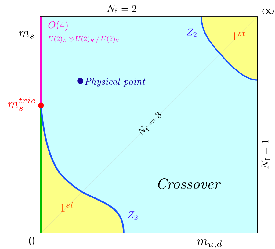
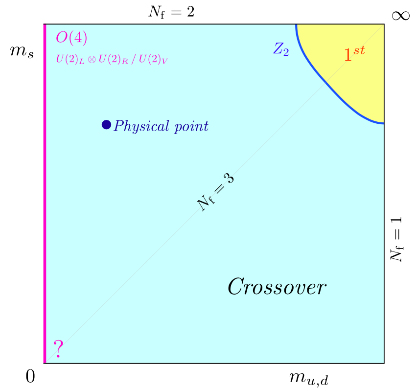
Figure 2.2: Columbia plot [left]. Alternative Columbia plot with a second-order transition in the 3-flavor chiral limit [right], as predicted in [37]. In this case, nothing is known yet about the universality class. Source [37].

For $N_{f}\geq 3$ massless quark flavors, according to these results, the chiral phase transition is expected to be of first-order. The diagonal of the Columbia plot corresponds to the case when all the three quark flavors, u, d, and s are degenerate with masses given by $m_{u}=m_{d}=m_{s}$. When all three quarks have a mass equal to the physical value of the light quark mass $m_{u,d}=m_{u}=m_{d}$, the transition is a crossover, but as the quark mass is decreased, one expects to hit a $Z(2)$ boundary - the blue line bounding the bottom-left first-order region painted yellow - at some critical mass value $m_{c}$ [36]. In this scenario, there is a tri-critical strange quark mass, where the chiral transition changes between first and second order. Viewing the strange quark mass as a smooth interpolator between $N_{f}=2$ and $N_{f}=3$ mass degenerate quarks, this corresponds to a situation with $N_{f}^{tric}<3$. For a recent review, we refer to [2].

An interesting and surprising prediction about the second-order nature of the 3-flavor chiral phase transition was made in [37]Philipsen_talk. This study considers a variable $N_{f}\in[2,8]$ for various lattice spacings and bare quark masses using unimproved Wilson gauge and staggered fermion actions. According to the findings of the previous lattice studies over the years, the first-order region shrinks with improved actions as well as with finer lattice spacings. In Reference [37], this shrinkage was found to continue to zero, leading to the definite existence of a tri-critical point. In the four-dimensional space of inverse gauge coupling $\beta$, bare quark mass $am$, $N_{\tau}$ and $N_{f}$, the bare critical masses $am_{c}$ form a $Z(2)$ critical surface which separates the first-order region from the crossover. Tri-criticality in the plane of bare critical quark mass $am_{c}$ and $N_{f}$ at a fixed lattice spacing $a$ translates to the existence of a $N_{f}^{tri}$ in the chiral limit; in the plane of $am_{c}$ and $N_{\tau}^{-1}$ – where $N_{\tau}$ is the temporal lattice extent related to temperature $T$ as $N_{\tau}^{-1}=aT$ – tri-criticality is encoded in $aT^{tri}$ on the $N_{\tau}^{-1}$ axis. Ref. [37] found $N_{f}^{tri}>6$, implying the disappearance of the bottom-left first-order region as shown in Figure 2.2 right.

Furthermore, Ref. [37] pointed out that the $N_{f}=3$ data generated using $\mathcal{O}(a)$-improved Wilson fermions [38] is also consistent with tri-critical scaling leading to a finite $aT^{tri}$ in the chiral limit, and hence a second-order transition in the continuum. The $N_{f}=3$ scenario has been recently investigated using Highly Improved Staggered Quark (HISQ) action Sharma_talk. The analysis [39] takes into account the temperature as well as the volume dependence of various chiral observables, such as 3-flavor chiral condensate, chiral susceptibility and observables constructed using some specific combinations of those two. Finally, employment of universal finite-size scaling techniques provides a 3-flavor chiral phase transition temperature for the non-vanishing value of lattice spacing to be $T_{c}=98^{+3}_{-6}$ MeV [39]Sharma_talk. Furthermore, no evidence for the first order phase transition is found in the pion mass range explored from 80 MeV up to a physical pion mass value of about 140 MeV, and the results are compatible with $3$-$d$ $O(2)$ universality class, and therefore with a second order phase transition in the 3-flavor chiral limit. Similarly, no evidence for a first-order transition is seen in the early results of a $N_{f}=3$ study using Möbius domain wall fermions with physical quark masses [40]. A recent 5-flavor study [41], based on Machine Learning approach – extensively discussed in Section 8 – finds a non-zero critical endpoint mass marking the boundary of a first-order region in the plane of $\beta$ and $am$, at a fixed temporal lattice extent of $N_{\tau}=6$. It would be interesting to see how this approach plays out in the four-dimensional space of $(\beta,am,N_{\tau},N_{f})$. Finally, new analytic studies of effective theories along the lines of [13], but using functional renormalization group [42] or conformal bootstrap [43] methods, also find the possibility of a second-order chiral transition for $N_{f}=3$ under certain conditions.

In conclusion, according to [37] Philipsen_talk, the continuum chiral phase transition is second-order for all $N_{f}\in[2,6]$, but no remarks could be made about the universality class of the chiral phase transition. It is also suggested that the phase transition might stay second-order up to the onset of the conformal window at $9\lesssim N_{f}^{*}\lesssim 12$. These studies connect naturally to the conformal window of strong interactions [44, 45, 46], to be further discussed in Section 5.

In [47], the importance of gauge degrees of freedom in producing a stable fixed point is emphasized, leading to a continuous transition for the antiferromagnetic $\mathrm{CP}^{N-1}$ models when $N\geq 4$. A standard Landau-Ginzburg-Wilson (LGW) field-theoretical approach, based on constructing a most general symmetry obeying effective Lagrangian using a gauge-invariant order parameter, predicts a first order transition in such a scenario, whereas numerical results do not sustain this mean field prediction. Furthermore, as pointed out in [48], ferromagnetic $\mathrm{CP}^{N-1}$ models in the large $N$ limit behave like an effective Abelian Higgs model for a $N$ component complex scalar field coupled to a $U(1)$ gauge field. This leads to the appearance of a stable fixed point with the possibility of a continuous transition, which again is in contrast to first order prediction of LGW. Possibly, all of the above arguments can be extended to finite temperature QCD for $N_{f}$ massless flavors, which might settle the disagreements between lattice simulations and theoretical mean-field predictions. We will return to this discussion in Section 28.

2.2.4   High Density Region

As discussed above, the region of high baryon density and lower temperatures is not accessible at the moment to lattice simulations of QCD. In this region we have to rely on functional approaches to QCD, or on low energy EFTs. Alternatively, one may opt to work in QCD-like models such as two-color QCD, or in some (unrealistic) region of the phase space: a dense isospin matter, with zero baryon density. In the following we discuss some examples of these different situations, to give a flavor of the current research.

EFTs with different degrees of sophistication are of course an important playground. Phenomena such as di-quark condensation and color superconductivity were discovered thanks to these analyses, see e.g. Ref. [49] for a classic review. A more recent comprehensive report is give in Ref. [50]. Topics that are close to the discussions on chiral symmetries are highlighted in Refs. [51, 52, 53]Sasaki_talk. A special emphasis is put on the manifestation of (partially) restored chiral symmetry via parity doubling of baryons and mesons in heavy-ion collisions and astrophysical observations.

There are important cases that do not suffer from sign problems on the lattice [54]: isospin dense matter, and QCD with two colors. Isospin symmetry is a $SU(2)$ rotation in flavor space (QCD interactions are flavor-blind) acting on up and down quarks. In the real world, isospin symmetry is explicitly broken by the (small) mass difference between up and down quarks. In lattice studies, up and down quarks are usually taken as degenerate and an appropriate chemical potential is introduced to create an isospin imbalance [55]. The phase diagram at a finite density of isospin has been studied on the lattice by various authors [56, 57, 58, 59]. An interesting feature – see Figure 2.3 – is that the critical line $T=T(\mu_{I})$ has a very small slope – it is almost horizontal. So, simulations performed at fixed temperature varying $\mu_{I}$ are very likely crossing the pion condensation line unless the temperature is really close to $T_{c}$. Note that in nuclear matter and in astrophysics isospin imbalance is very important, but smaller than the baryon one. Lattice studies [60, 56, 61, 59, 62, 63] which consider $\mu_{I}\neq 0,\mu_{B}=0$ are thus to some extent artificial, but still interesting: for instance, one can observe (1) signatures of the superconducting BCS phase expected on perturbation theory grounds, and (2) the role of pion condensation in the early universe evolution at nonvanishing lepton flavor asymmetries [64, 60]Cuteri_talk.

Two-color QCD is free from the sign problem at nonzero baryon density thanks to its enlarged chiral symmetry: from the $SU(N_{f})\times SU(N_{f})\times U(1)_{B}$ to $SU(2N_{f})$. Intuitively, baryon and isospin are basically the same symmetry for two colors. For this reason, di-quarks are stable in two color QCD. Studies of two color matter have been reported in [65, 66, 67, 68, 69, 70, 71, 72, 73, 74]. These studies have confirmed that baryonic matter forms at an onset $\mu_{o}=m_{\pi}/2$, whereupon matter is superfluid. Current studies focus on the understanding of lattice artifacts, [74], Bornyakov_talk. High quality lattice data allow the study of the interrelation between different pairing patterns, chiral symmetries and gauge dynamics, including signatures of deconfinement.

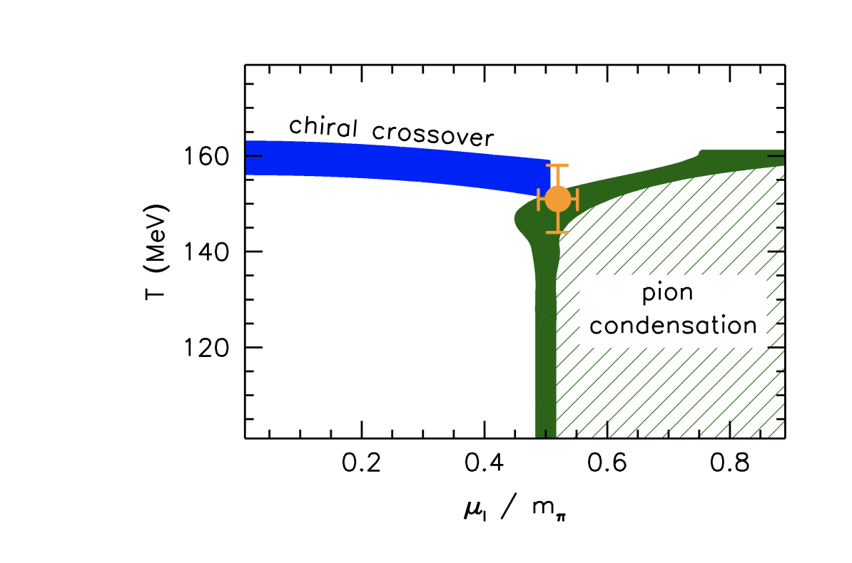
Figure 2.3: Lattice results for the phase diagram of QCD in the temperature-chemical potential for isospin plane, from Ref[56].

Finally, one may consider a chemical potential, $\mu_{5}\equiv(\mu_{R}-\mu_{L})/2$ associated with the non-conserved axial current, $\bar{\psi}_{i}\gamma_{5}\psi$ [75]. Early lattice studies of chiral density were performed having in mind a toy model for the chiral magnetic effect in heavy ion collisions [76]. One first systematic study of the phase diagram at equilibrium appeared in Ref. [75]. Since then the field is developing, also due to the relation with the elusive Chiral Magnetic Effect [77]. Since the axial current is not conserved, the associated chemical potential, and the related results, need to be taken with some care.

2.3   The Road Ahead

The analysis of the symmetries, their patterns, and the imprints on the phenomenology of the related critical points remain an important subject, with several open issues. In particular, we have seen that the nature of the phase transition as a function of the number of flavors, and the fate of the axial symmetry are under debate. The nature of the transition with increasing $N_{f}$ has also a potential relevance for phenomenology, as models for strong electroweak breaking often capitalizes on the strong first order transition expected for large $N_{f}$. Theoretically, if indeed a second order transition persists till the conformal window, we will have to understand how a 3D infrared fixed point would morph with 4D conformality. This latter point – the fate of the anomaly – is related to the topological aspects of QCD, which will be further discussed in Section 5.

Figure 1 shows that, besides the theoretical interest, the chiral behavior in QCD may well constrain the phase diagram, in particular, the location of the critical point at non-zero density which we will discuss in the Sections 3, 5.

There is a growing interest in the approximate $SU(4)$ symmetry observed at high temperatures. We may speculate that quarks and gluons are not the right degrees of freedom for the quark-gluon plasma (QGP) because they are not compatible with this symmetry. Should this be true, it would question all the present transport approaches, which will be further discussed in Section 3. The crossover from $SU(4)$ symmetry to the $SU(2)XSU(2)$ symmetry of the QGP occurs at a temperature of about 300 MeV, close to another crossover of an apparent different nature. An open question is to understand whether there is a common origin. Several hypotheses have been put forward, none of them completely satisfactory yet. One important aspect of future research is to clarify this point.

Finally, much of the discussions in this section were focused on chiral symmetry. A proper definition of confinement, and its relation, if any, with chiral symmetry, is an important theoretical open problem, going beyond the scope of this review. Here we just note that steps in this directions require analysis of gauge dynamics, and several studies focusing on monopole dynamics, flux tubes and their interrelation with the static potential have appeared, see e.g. [78, 79]Kudrov_talk. These analyses may also help in understanding the nature of a threshold in the Quark Gluon Plasma at a temperature of about 300 MeV.

It is of crucial importance for our final understanding of QCD under extreme conditions that all the issues discussed are clarified. Although the results are still not fully conclusive they clearly indicate the research priorities in QCD under extreme conditions in the next future.

3   Nature and Phenomenology of the Quark-Gluon Plasma

Strong interaction matter under extreme conditions can be formed in laboratory: see e.g. [80] for an authoritative overview, as well as the Proceedings of the Quark Matter Conference for updates. A rich and clear discussion with focus on relevant experimental observables for understanding the phase structure of QCD at high $\mu_{B}$, including a region which is difficult to study on the lattice, can be found in Ref. Galatyuk_talk.

In this section, we will discuss the region which is still accessible to lattice studies. In particular, the focus is on the search for the much wanted QCD critical point. This has motivated a dedicated collaboration, the Beam Energy Scan Theory (BEST) collaboration Ratti_talk. The BEST Collaboration "will construct a theoretical framework for interpreting the results from the ongoing Beam Energy Scan program at the Relativistic Heavy Ion Collider (RHIC). The main goals of this program are to discover, or put constraints on the existence, of a critical point in the QCD phase diagram, and to locate the onset of chiral symmetry restoration by observing correlations related to anomalous hydrodynamic effects in quark gluon plasma.". The WEB page of the BEST Collaboration provides important information, which is reviewed later in this Section.

Central in this discussion is the role of fluctuations: lattice results on fluctuations are reviewed in the next Subsection. Phenomenological applications of lattice studies are discussed next. Let us single out here a specific point: the calculation of spectral functions. Spectral functions are an important input for phenomenology; unfortunately their calculation poses specific technical problems, which are discussed in a dedicated Section 4. Before turning to lattice results, we would like to mention the cosmological aspects of high temperatures. Temperatures of cosmological relevance may not be accessible in numerical simulations (see however Sec. 6), but they are amenable to analytic studies or numerical simulations in dimensionally-reduced EFTs. They access phenomena of enormous relevance, including the thermal production of gravitational waves or the existence of electroweak phase transitions beyond the Standard Model. Strictly speaking, this goes beyond the scope of the report, which focuses on strong interactions, however, the two fields are next to each other and may be bridged by thermal perturbation theory [81, 82, 83]Ghiglieri_talk,Schicho_talk.

3.1   Fluctuations

Fluctuations are important probes of a phase transition. They are expected to grow large in the critical region, and the lattice results may be contrasted with predictions from different universality classes [84]Guenther_talk.

Most importantly, they can also offer a starting point to construct various quantities that can be compared to measurements from heavy ion collision experiments.

Fluctuations are defined as the derivatives of the pressure with respect to various chemical potentials:

$$\chi^{B,Q,S}_{i,j,k}=\frac{\partial^{i+j+k}(p/T^{4})}{(\partial\hat{\mu}_{B})^{i}(\partial\hat{\mu}_{Q})^{j}(\partial\hat{\mu}_{S})^{k}}\,,\ \hat{\mu}=\frac{\mu}{T}$$ (3.1)

While fluctuations to various order have previously been published on finite lattices for example in Ref. [85, 86, 87, 88, 89], now new continuum extrapolated results are available in Ref. [90, 91]. These results are obtained by the Taylor method and continuum extrapolated from lattices with temporal extend $N_{t}=6,8,12$ and 16 with HISQ fermions. The precision of these results is high enough to allow for a comparison to different models with detailed studies for example on the inclusion or exclusion of various states in a Hadron Resonance Gas (HRG) model. To match the lattice results, for example for $\chi^{BS}_{11}$, it is necessary to add states from quark models to the list of resonances from the PDG [92]. On the other hand in Refs [93, 94] the coefficients of the fugacity expansion from imaginary chemical potential

$$\frac{p}{T^{4}}=\sum_{j=0}^{\infty}\sum_{k=0}^{\infty}P^{BS}_{jk}\cosh(j\hat{\mu}_{B}-k\hat{\mu}_{S})$$ (3.2)

are presented. The results are continuum estimates obtained with stout smeared staggered fermions on $N_{t}=8,10$ and 12 lattices. The analysis is based on a two dimensional fugacity expansion with imaginary $\mu_{B}$ and $\mu_{S}$. The $P^{BS}_{21}$ coefficient includes contributions from $N-\Lambda$ and $N-\Sigma$ scattering where the negative trend indicates the presence of an repulsive interaction that cannot be described with the addition of more resonances.

Lattice data can also be used as input for parametrizations as done for example in [95, 96]. The lattice input is especially well suited for the temperature range around the crossover between the hadronic phase that can often be described by the HRG and the QGP-phase.

Moreover, lattice data for fluctuations at low and vanishing density serve as benchmark results for functional QCD computations of fluctuations and that in QCD-assisted EFTs, [97, 98, 99]Pawlowski_talk. This allows for an extrapolation of low density lattice results to larger densities, including the regime of the potential critical end point.

As stated at the beginning of this Section, the ratios of various fluctuations can be used to start a comparison between heavy ion collision experiments and lattice QCD results. The ratios of various fluctuations can be used to express the cumulants of the Baryon number distribution. This offers an observable for comparisons with heavy ion collision measurements of the proton number distribution. At the current precision level this can only be a rough comparison. These cumulants have been published in Refs. [88, 89, 93]. If the precision is further increased in the future, other effects should be taken into account, like the continuum limit on the lattice side, or volume fluctuations and non-equilibrium effects on the experimental side (see for example Ref. [100]). However, if the comparisons are done with the necessary care, a deviation between the extrapolated results from the lattice and the experimental measurements can be a hint, that the physics in that area is longer described by an analytic function.

3.2   Equation of State

The equation of state is an important quantity both from the purely theoretical point of view as well as input quantity to various models which describe the Quark Gluon plasma. The equation of state at vanishing baryochemical potential $\mu_{B}$ is known from lattice QCD simulations in the continuum limit (Refs. [101, 102, 103]) up to high enough temperatures to be matched to perturbative results (Refs. [104, 105, 106]). Its continuation to finite density has posed a significant challenge for several years. When extrapolated to finite $\mu_{B}$ with a Taylor expansion up to $\mu_{B}^{6}$ it shows an increase in the error around the transition temperature, which leaves room for unexpected behavior. This has been observed by different groups and on different data sets (Refs. [87, 107]) and with new high precision data (Ref. [91]) one can observe an increase of the difference between the expansion up to $\mu_{B}^{4}$ and $\mu_{B}^{6}$. Some resummation methods (Refs. [107, 108]) hope to mitigate this influence. A comparison in a small volume with direct methods (Ref. [108]) shows, that the unexpected behavior does not appear with either the new resummation schemes or higher orders and high precision of the Taylor expansion.

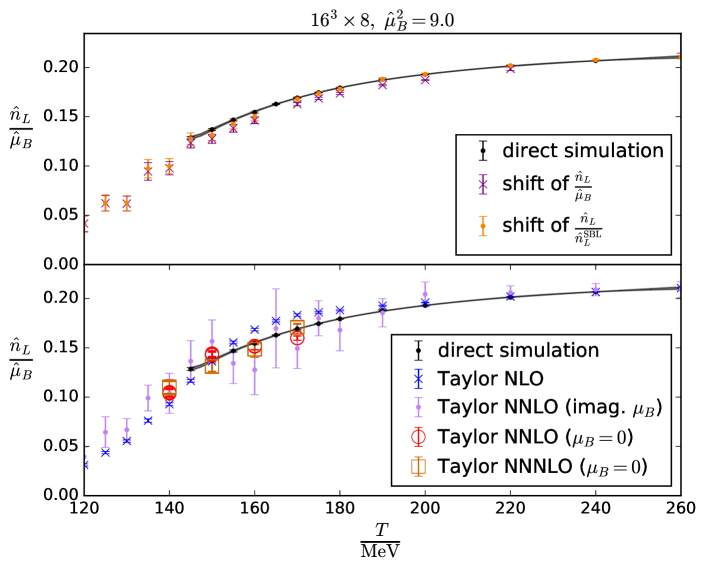
Figure 3.1: (Ref. [108]) Comparison of different extrapolation approaches with direct results on a fixed lattice and in small volume.

3.3   Influence of a Magnetic Field

When trying to match the situation in heavy-ion colliders, an additional important influence on the phase transition is driven by the magnetic field generated in non-central collisions [109, 110, 111]. The simulation of QCD with a magnetic field on the lattice has been a very active field in the last decade (see, e.g. Refs. [112, 113, 114, 115, 116, 117, 118, 119, 120, 121]). Early results, not yet extrapolated to the continuum limit, showed an increase of the transition temperature as a function of the magnetic field intensity $B$; this agreed well with the expectation resulting from the so-called magnetic catalysis, which describes that at zero temperature chiral symmetry breaking is enhanced by the magnetic field. However, properly continuum extrapolated results revealed a drop of the transition temperature as a function of $B$, an effect which is related to the so-called inverse magnetic catalysis, i.e., the decrease of the chiral condensate in a growing magnetic field for temperatures around and above $T_{c}$ [113]. Such a phenomenon induces, furthermore, a strengthening of the crossover, making the gap in the observables between the different phases higher and steeper. This effect was predicted to result, eventually, in the appearance of a real, first order phase transition for magnetic field intensities of the order of $eB\sim 10$ GeV² [122]. Furthermore, studies with various pion masses (Refs. [123, 119]) suggested that the decrease of the pseudocritical temperature with $B$ could be a deconfinement (rather than chirally) driven phenomenon. Indeed, the magnetic field was shown to affect confinement properties, making the string tension anisotropic, in many studies [124, 125, 126].

Very recent lattice results on chiral and confinement properties of $N_{f}=2+1$ QCD at the physical point in both the vanishing and high temperature cases have been obtained in the presence of unprecedented strong magnetic fields, namely $eB=4$ and $9$ GeV² [127, 128] Maio_talk. Concerning chirality, it was shown that magnetic catalysis maintains its linear behavior in $eB$ in the zero temperature regime, fitting very well to the lowest Landau level prediction. Moreover, the onset of inverse magnetic catalysis is driven to lower and lower temperatures as the magnetic field grows, leading to a drop in the transition temperature larger than expected. Thus, the QGP can be found down to temperatures as low as ${\sim}\,60$ MeV in a $eB=9$ GeV² magnetic background. Moreover, in the $9$ GeV² magnetic field simulations, the authors noticed the transition region being extremely narrow. Thus, a deep study on the nature of the transition was performed, through dedicated simulations, providing the first evidence for a first order phase transition of $N_{f}=2+1$ QCD at the physical point in a magnetic background.

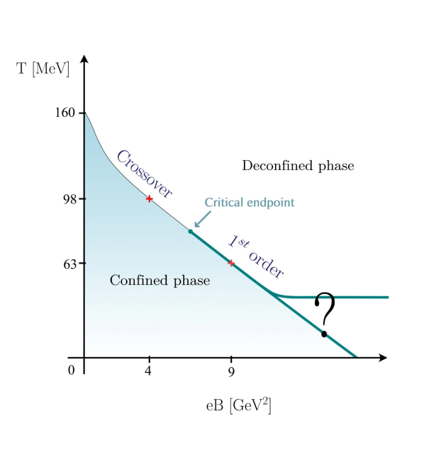
Figure 3.2: Updated QCD phase diagram in an external magnetic field, based on new facts that emerged in [127, 128]. The (pseudo)critical temperature continues its steady drop as a function of B, and the transition switches from a crossover to first order at a critical end point located in the range $4$ GeV${}^{2}<eB_{E}<9$ GeV² (or alternatively $65$ MeV$<T_{E}<95$ MeV). The fate of the critical temperature in the asymptotic magnetic field limit remains an open question.

On the confinement side, previous work suggested an anisotropic deconfinement [125] in the zero temperature regime for magnetic fields ranging up to $eB=4$ GeV². It was shown that this prediction is not verified and, furthermore, such a partial deconfinement does not happen even for the largest explored magnetic background, i.e. $eB=9$ GeV² [127]. The authors also studied the confining potential at finite temperature around the phase transition found in [128]. They found, as expected, that the chirally broken phase exhibits confinement in all the directions, while the chirally restored phase appears to be deconfined. To summarize all findings reported above, they proposed an updated version of the $N_{f}=2+1$ QCD phase diagram at the physical point, as can be seen in Fig. 3.2.

The effects of a magnetic field are an active topic [129, 130, 131, 132]. In addition to studying a magnetic field at zero or finite temperature, also systems where a background magnetic field is considered in combination with a finite density [133, 129, 130] or a finite rotation [134, 135, 136] are, currently, under investigation. Moreover, recently, also inhomogeneous magnetic backgrounds are taken into consideration because of their phenomenological relevance in the context of heavy-ion scattering experiments [137].

3.4   BEST Efforts

While a direct comparison between lattice and experiments is challenging, lattice data can also serve as input or benchmark for hydrodynamic evolution models. The matter created in heavy-ion collisions can be well-described by relativistic viscous hydrodynamics, which can provide a framework to search for the QCD critical point if modified to take critical phenomena into account. The BEST-collaboration combines first-principles lattice QCD calculations and phenomenological approaches, to create a framework for the analysis of experimental data at low collision energies Ratti_talk,[138]. They computed an equation of state that reproduces the lattice QCD one up $\mathcal{O}(\hat{\mu}_{B}^{4})$ and contains a critical point in the 3D Ising model universality class [139] from which they can compute the thermodynamic quantities at various chemical potentials (for example with the strangeness neutrality setting [140]). The equation of state can then be used as an input for hydrodynamical simulations.

To definitively claim or rule out the presence of a QCD critical point or anomalous transport requires a comprehensive framework for modeling the salient features of heavy ion collisions at BES energies, which allows for a quantitative description of the data. BEST developed initial conditions, which connect the pre-equilibrium stage of the system to hydrodynamics on a local collision-by-collision basis [141, 142, 143]. A quantitative understanding of fluctuations near the critical point needs to be developed as well. In fact, the evolution of the long wavelength fluctuations of the order parameter field close to the critical point is not captured by hydrodynamics. Two approaches have been followed within BEST: a stochastic approach with noise [144], and a deterministic approach in which correlation functions are treated as additional variables, together with the hydrodynamics ones [145]. The numerical implementation of the latter are underway [146, 147].

The efforts of the BEST-collaboration also include the particlization after the hydrodynamic phase. The aim is to develop an interface between the hydrodynamic evolution model and the hadronic transport phase, in a way that it preserves fluctuations (see Refs. [148, 149, 150]).

3.5   Transport Properties

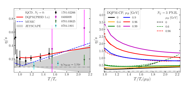
Figure 3.3: Specific shear viscosity as a function of the scaled temperature $T/T_{c}$ at $\mu_{B}=0$ (left) and at finite $\mu_{B}$ (right). The symbols corresponds to the lQCD results for pure SU(3) gauge theory (black squares) [151], (green triangles and magenta circles) [152], (cyan stars) [153]. The dash-dotted gray line demonstrates the Kovtun–Son–Starinets bound $(\eta/s)_{KSS}=1/(4\pi)$ [154]. The grey area represents the model-averaged results from a Bayesian analysis of experimental heavy-ion data [155]. The red line corresponds to the DQPM results [156], while the dashed blue line displays $\eta/s$ parametrization used in hydrodynamic simulations within MUSIC in [143]. The model results, obtained by the RTA approach with the interaction rate, for finite $\mu_{B}$: DQPM-CP results [157](solid lines) are compared to the estimates from the $N_{f}=3$ PNJL model (dashed lines) [158] as a function of scaled temperature $T/T_{c}(\mu_{B})$.

Experimental and phenomenological aspects of transport are discussed in depth in Ref. Soloveva_talk. The evolution of the QGP phase has been successfully described within hybrid approaches based on relativistic hydrodynamics and transport theory, such as iEBE-VISHNU [159], vHLLE + UrQMD/SMASH [160, 161] and MUSIC+UrQMD [162, 143]. Nevertheless, some advanced transport approaches, such as AMPT [163] and PHSD [164, 165] can provide the whole evolution of HIC, including the QGP phase. In order to perform hydrodynamical simulations of the time evolution of the quark-gluon matter at finite baryon chemical potential, one needs to estimate first the EoS and the transport coefficients of the matter in this region. The transport coefficients depend on the underlying microscopic theory which describes the interaction between quarks and gluons, however, it is notoriously difficult to evaluate microscopic properties of the QGP matter at finite $T$ and $\mu_{B}$ from first principles. Transport coefficients serve as a bridge between the microscopic transport and hydrodynamics approaches. One can evaluate the transport coefficients by methods of kinetic theory and apply them in the hydrodynamical simulations.

To examine transport coefficients at finite $\mu_{B}$ where the phase transition is possibly changing from a crossover to a 1st order one it is necessary to resort to effective models which describe the chiral phase transition. While most of the effective models have similar equations of state (EoS), which match well with available lattice data, the transport coefficients can vary significantly already at $\mu_{B}=0$ [166, 167, 168, 169, 165, 158, 170]. Therefore, it would be beneficial for the hydrodynamic and transport simulations of the strongly interacting matter for the moderate and high $T$ and $\mu_{B}$ to have predictions for transport coefficients from lQCD calculations in this region of the phase diagram.

The transport coefficients of the QGP medium have been computed for a wide range of baryon chemical potential for two models with a similar phase structure: the extended $N_{f}=3$ Polyakov Nambu-Jona-Lasinio (PNJL) model and Dynamical QuasiParticle Model with a CEP (DQPM-CP), where the hypothetical CEP located at $\mu_{B}=0.96$ GeV.
The specific shear viscosity for the QGP phase is shown in Fig. 3.3 as a function of scaled temperature $T/T_{c}$ at $\mu_{B}=0$ (left) and at finite $\mu_{B}$ (right). At $\mu_{B}=0$ we show results from the DQPM [156] (solid red line), in comparison with the lQCD results for pure SU(3) gauge theory [151, 152, 153], model-averaged results from a Bayesian analysis of the experimental heavy-ion data [155] (grey area) and $\eta/s$ employed in hydrodynamic simulations in [143] (dashed blue line). For finite $\mu_{B}\geq 0$ we show the results from the PNJL model and DQPM-CP models obtained by the RTA approach with the interaction rate. The estimations from both models show an increase of specific shear viscosities $\eta/s$ and electric conductivities $\sigma_{QQ}/T$ with $\mu_{B}$. While the specific shear viscosities are in agreement for moderate $\mu_{B}$ in the vicinity of the phase transition, there is a clear difference in the electric conductivity essentially due to the different description of partonic degrees of freedom [157].

Furthermore, it has been found that for fixed $\mu_{B}$, where the phase transition is a rapid crossover, transport coefficients show a smooth temperature dependence while approaching the (pseudo)critical temperature from the high temperature region. The presence of a first order phase transition changes the temperature dependence of the transport coefficients drastically.

In order to take into account a proper non-equilibrium description of the entire dynamics through possibly different phases up to the final asymptotic hadronic states, a microscopic treatment is needed. The Parton-Hadron-String Dynamics (PHSD) transport approach [171, 164, 172, 165] is an off-shell transport approach based on the Kadanoff-Baym equations in first-order gradient expansion which allows for simulations of both the hadronic and the partonic phases. The microscopic properties of quarks and gluons are described by the DQPM with a crossover phase transition, where the microscopic characteristics of partonic quasiparticles and their differential cross sections depend not only on temperature $T$ but also on the chemical potential $\mu_{B}$ explicitly. We find that HICs results from the extended PHSD transport approach, where in QGP phase we found that transport coefficients have noticeable $T$ and $\mu_{B}$ dependence, have been in agreement with the BES STAR data in case of bulk observables and elliptic flow of charged particles [173], and reasonably agrees with the results from hybrid approach [143]. It is important to note that, $\eta/s$ used for hydrodynamic evolution is close to the DQPM estimations as shown in Fig. 3.3 (left). However, results from the PHSD transport approach have shown rather small influence of the $\mu_{B}$-dependence of the QGP interactions on the elliptic flow than hybrid simulations [165, 173]. This small sensitivity of final observables to the influence of baryon density on the QGP dynamics can be explained by the fact that at high energies, where the matter is dominated by the QGP phase, one probes the QGP at a very small baryon chemical potential $\mu_{B}$, whereas at lower energies, where $\mu_{B}$ becomes larger, the fraction of the QGP drops rapidly. Therefore, the final observables for lower energies at order of $1-10$ GeV are in total dominated by the hadrons which participated in hadronic rescattering and thus the information about their QGP origin is washed out or lost.

3.6   Experimental Efforts

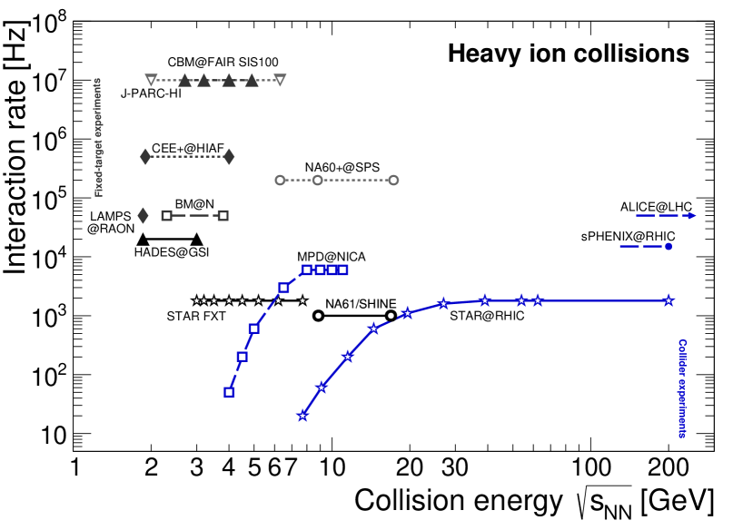
Figure 3.4: Overview over future and past experiments taking data from heavy ion collisions [174, 175, 176].

There is a huge experimental effort to study the QGP specifically with dileptons Galatyuk_talk. Similar as on the theory side, the search for a first order transition and a possible QCD critical endpoint are important research points as well as the general properties of QCD matter around a deconfinement and/or chiral transition. In the near future many experiments are expected to take high statistic data (see figure 3.4 from Ref. Galatyuk_talk) which will allow new inside from statistic hungry probes like dileptons and photons. Dileptons for example allow answering the fundamental questions related to the mechanism of chiral symmetry restoration in QCD matter and the transition from hadronic to partonic degrees of freedom, the total lifetime of the interacting medium and its average temperature, the evolution of collectivity and the nature of the electromagnetic emission, as well as the transport properties of the medium (i.e., the electrical conductivity).

3.7   The Road Ahead

We close the Section with a summary of the lattice issues which the phenomenological/experimental community considers most urgent:

1. The study of fluctuations to identify phase transitions and a possible QCD critical point should be further pursued. As it clearly appeared from the previous discussion, this requires vigorous collaboration between experiments and theoretical work. An important contribution is expected from lattice investigations, but these are hampered by the so-called sign problem, which actually dominates the region of interest in the phase diagram. The solution (or at least an effective mitigation) of the sign problem is thus crucial: this point is addressed in Section 4. It has to be noted that even existing methods may be stretched to reach the a region candidate for the critical endpoint.

   Moreover, functional approaches (FA) to QCD offer direct computational results at larger densities. In particular, they can be understood as $mu_{B}$-exptrapolations of lattice results at lower densities with the maximal dynamical information of QCD in comparison to other extrapolations. This opens a promising route toward a combined LFT-FA analysis of the high density regime of QCD.

2. The equation of state should be provided for a broad range in temperature and baryon chemical potential. Also, the influence of other parameters like a strangeness chemical potential or a magnetic field should be explored. On the one hand, this could allow a closer comparison to heavy ion collisions where a magnetic field is present especially in off-central collisions as well as strangeness fluctuations if an overall equilibrium is not reached. On the other hand, these parameters offer more theoretically interesting regimes. There is for example hints a critical end point at high magnetic fields (Ref. [128]).

3. Essential for all phenomenological approaches are the temperature dependence of the pole masses of pseudo scalar and vector bosons with zero or finite momentum. This has been partially accomplished however it requires a solid understanding of spectral functions for the identification of pole masses.

4. There are measurements of transport coefficients of heavy quarks in the medium like $D_{s}$ but the results from different lattice groups do not agree (maybe because quenched and not quenched approaches give different results). In addition, in the transport approaches we need these coefficients at finite momentum of the heavy quark (with respect to the medium). An improvement in this situation would be welcomed. These issues call also for methodological improvements in the computation of spectral functions which will be reviewed in Section 4.

5. Another quantity we should urgently know is the pole mass and stability of protons as a function of the temperature. Work in this direction has been done in Ref. [177], however, limited to the pole mass. Information on the stability would be important as well. To settle this with a physical pion mass would be of great help.

6. A precise determination of the density (baryon, strangeness) as a function of the temperature - namely of the first derivative of the partition function - would be important. This would allow us to establish ( what also Nambu-Jona-Lasinio models predict) whether the hadronization temperature of strange quarks differs from that of light quarks.

7. Any information about the underlying degrees of freedom of a QGP would be of great help. Recent work on unusual symmetries (Ref. [25]), already mentioned in Section 2 should be further explored.

4   Methodological Challenges: Spectral Functions and Sign Problem

While lattice QCD has been quite successful at Euclidean space-time geometry and zero chemical potential over the past decades, it suffers from severe limitations when it comes to the calculation of expectation values at non-zero baryon number density or quantities related to real time. This is due to the fact that lattice QCD calculations crucially rely on the interpretation of the Boltzmann factor as a probability density for the numerical sampling of the path integral. Once the Boltzmann factor is no longer strictly positive, or even becomes genuinely complex, this interpretation is lost and standard Monte Carlo methods for the calculation of the path integral cease working. This is called the QCD sign problem. To deal with or to circumvent the sign problem and to reach out to the expected QCD critical point bears huge methodological challenges. Similarly, this is true for the calculation of spectral functions, which provide a way to extract, e.g., transport coefficients, but are also of interest for many other reasons (for example, also at zero temperature several observable quantities are related to spectral densities). In the following, we will discuss some of those challenges in more detail.

4.1   Spectral Functions as an Inverse Problem

Before entering the details of the inverse problem, we would like to mention an important aspect of functional Renormalization Group studies: fRG can be formulated in real time, via a combination of the fRG approach and the formalism of Schwinger-Keldysh path integral, see e.g. [6] for a recent review. The spectral functions thus obtained may be contrasted with lattice results. In this case, the sign problem will be solved from scratch, completely bypassing the difficult inversion procedure, which will be the focus of the remaining part of the discussion.

The computation of spectral functions begins with lattice correlators [178, 179]. It is an ill-posed or at least ill-conditioned problem as the task is to reconstruct salient features of the spectral functions (peaks, typically) from a smooth function that is only known in a limited amount of points, with limited accuracy.

Bottomonium has been used as an important case study [180, 181]: first, it is of great physical interest due to the rich production at the LHC. Secondly, the inversion required to compute spectral functions is a “simple” inverse Laplace transform, for which a wealth of methods has been designed. Lattice studies predict the sequential suppression of bottomonium in the QGP, which has been observed in experiments [182]. Despite qualitative coherence among the results, a quantitative agreement has not been reached yet. A comparison of the different methods may be found in Ref.[183].

The numerical inversion of the Laplace transform on the real axis is an inverse and ill-posed problem. Usually, methods for the inversion problem require the evaluation of the Laplace function F on some knots; this could be an issue if a closed form of F is not available. In lattice QCD applications, the Laplace transform is known only on pre-assigned samples or measures (and with errors) and an accepted strategy is to design fitting models able to represent this function Allton_talk.

Before entering the details of the inverse problem, we would like to mention an important aspect of functional Renormalization Group studies: fRG can be formulated in real time, via a combination of the fRG approach and the formalism of Schwinger-Keldysh path integral, see e.g. [6] for a recent review. The spectral functions thus obtained may be contrasted with lattice results. In this case, the sign problem will be solved from scratch, completely bypassing the difficult inversion procedure, which will be the focus of the remaining part of the discussion.

Ref. Cuomo_talk is a mathematical introduction to inverse Laplace transforms aimed at physicists. Besides a comprehensive discussion of different methods, many of them not yet tried in this context, it presents the main numerical issues about the Laplace inversion formulas in the discrete data framework and discusses how to estimate the main sources of errors. Very important in this context is the interpolation of a discrete data set. This latter point is discussed in Ref. Conti_talk, another mathematical review prepared for a physics audience. Spline models have been widely used in many areas of science and engineering, such as signal and image processing, computer graphics, deep learning, neural networks, or data representation, as important tools to model and predict data trends. Ref. Conti_talk aims at providing an introduction to basic spline models-smoothing, regression, and penalized splines-based on polynomial splines but also on exponential-polynomial splines. The latter are particularly suitable for data showing exponential trends as in the framework of the Laplace transform inversion. In particular, Ref. Conti_talk discusses HP-splines, a recently defined penalized regression model, generalization of P-spline, in which polynomial B-splines are replaced by hyperbolic-polynomial bell-shaped basis functions, and a suitably tailored penalization term replaces the classical second-order forward difference operator.

4.2   Spectral Functions and Effective Field Theories

Most important for the control of the results, and to monitor the approach to the continuum limit, is the interface between lattice and effective field theories. Nonperturbative correlators emerge in the nonrelativistic effective field theory (NR EFT) factorization [184] that should be calculated on the lattice. Ref. Brambilla_talk presents lattice calculation of some of these.

In particular, the EFT called potential nonrelativistic QCD (pNRQCD) at finite temperature [185] gives a framework to define the potential, calculate it and systematically calculate energy levels and widths [186]. Calculations have been made in (resummed) perturbation theory and then used to compare and check lattice results, for example in the case of the Polyakov loop and the Polyakov correlator [187, 188] establishing the region in which the screening regime is active.

Moreover, combining pNRQCD and an open quantum system [189], it is possible to describe the nonequilibrium evolution of small quarkonia systems (bottomonium) inside the strongly coupled Quark Gluon Plasma with an evolution equation for the singlet and octet density matrix of the Lindblad type on the basis of two transport coefficients defined as appropriate correlators of electric fields at finite temperature [190, 191]. In this way, the EFT works as an intermediate layer that allows to use lattice QCD equilibrium input to study the nonequilibrium evolution of bottomonium inside the QGP. One can also relate these transport coefficients to the thermal modification of the energy levels and to the thermal widths of quarkonium, which allows us to use unquenched lattice calculations of the thermal modification of the mass and the width of quarkonium [192] as input. Gradient flow is particularly suitable for the direct lattice calculation of these transport coefficients [193, 194]. Besides the methodological importance, these studies also provide an important input to phenomenology as already mentioned. The same interface between NR EFTs and lattice may be used to study a number of problems ranging from the study of the exotics X Y Z [195, 196] to quarkonium production [197]. This novel alliance of EFTs and lattice, with lattice correlators defined inside the EFT appears to be a novel and promising avenue.

4.3   QCD at Non-Zero Density: From Taylor Expansions to Lee–Yang Zeros

The Taylor expansion method [198] is one of many approaches to circumvent the QCD sign problem and has been very successful in the past. Although limited to small baryon chemical potentials $\hat{\mu}_{B}\equiv\frac{\mu_{B}}{T}\lesssim 2$, some results close to the continuum limit have been presented on the QCD equation of state [87, 107], the curvature of the transition line [8, 9] and fluctuations of conserved charges [89, 90]. The main idea is the expansion of the dimensionless pressure $p/T^{4}$ in terms of the three chemical potentials for baryon number, strangeness and electric charge, $\hat{\mu}_{B},\hat{\mu}_{Q}\hat{\mu}_{S}$,

$$\frac{p}{T^{4}}=\sum_{i,j,k}\frac{1}{i!j!k!}\chi^{B,Q,S}_{i,j,k}\hat{\mu}_{B}^{i}\hat{\mu}_{Q}^{j}\hat{\mu}_{S}^{k}\;,$$ (4.1)

where the expansion coefficients are defined as in Eq. (3.1). The series is even, i.e., the summation runs over all $\{i,j,k\}$ with $(i+j+k)\;\text{mod}\;2=0$. It is very tempting to estimate the radius of convergence of the expansion above since, by definition, the radius would be limited by the elusive critical point in the QCD phase diagram. However, the limiting singularity can also be located in the complex $\hat{\mu}_{B}$ plane. A famous example are the Lee-Yang edge singularities [199], in the context of lattice QCD and the QCD phase diagram first discussed by [200, 201]. Estimating the radius of convergence from the lattice results of the Taylor coefficients $\chi^{B,Q,S}_{i,j,k}$ is very challenging, due to the limited number of coefficients, usually $(i+j+k)\leq 8$, and the increasing statistical error. A simple rational estimator has been used frequently in the past [202, 87], even though it is known to converge slowly [203].

A discussion of Taylor expansions in (2+1)-flavor QCD for the pressure, net baryon number and the variance of the distribution on net-baryon number fluctuations is given in [91], Karsch_talk. The authors obtain series expansions from an eighth-order expansion of the pressure, Eq. (4.1), which is re-summed by a $[2,2]$ and $[4,4]$ diagonal Padé. The poles of those Padés correspond to the Mercer-Roberts estimator [204] of the radius of convergence. The poles are indeed located in the complex $\hat{\mu}_{B}$ plane as shown in Fig. 4.1 (left) and show an apparent approach to the real $\mu_{B}$ axis with decreasing temperature.

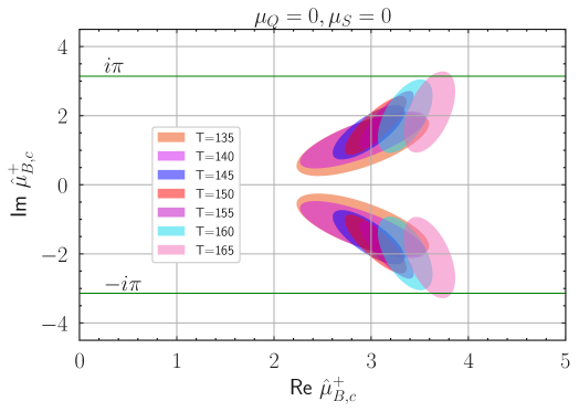
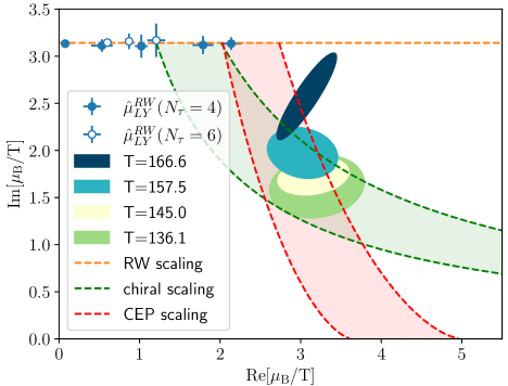
Figure 4.1: Poles in the complex $\hat{\mu}_{B}$ plane from the $[4,4]$-Padé re-summation of the Taylor series about $\hat{\mu}_{B}=0$ (left) and from the multi-point Padé approach applied to lattice QCD data at imaginary $\mu_{B}$ (right). Also shown in the right panel is the expected scaling behavior of the Lee-Yang edge singularities for different critical points, indicated by dashed lines/bands.

Corresponding results for a re-organized expansion with zero net strangeness ($n_{S}=0$) are also discussed.

Due to the limited number of Taylor coefficients one has at hand for the series about $\mu_{B}=0$, one needs strategies to compute the Lee-Yang zeros from multi-point Padé approximants obtained from simulations at imaginary $\hat{\mu}_{B}$ [205, 206], Schmidt_talk. This may be achieved by combining continuation from imaginary chemical potential via Padé approximants[207, 208] with Taylor expansion. Analytic continuation in combination with Taylor expansion was proposed in Refs. [209, 210]. For further interesting resummation schemes see [211]. The results are shown in Fig. 4.1 (right). Also shown is the expected scaling behavior of the Lee-Yang edge singularities associated with the Roberge-Weiss, the chiral and the QCD critical point. Interestingly, at temperatures close to, but below the Roberge-Weiss transition temperature ($T\lesssim T_{RW}$) the poles follow the expected Roberge-Weiss scaling. At temperatures $T\lesssim$ 170 MeV, a qualitative change in the behavior of the singularities is found: they start to approach the real axis. If it can be established that the scaling behavior follows the one expected for the QCD critical point, the location of the QCD critical point can be determined by a scaling analysis.

This method has been successfully applied in the Gross-Neveu model [212], see also [213] for further investigations in low energy EFTs with and without fluctuations see [214, 213, 215, 216, 217]. In particular, the scaling behavior of the location of the edge singularity has been established in [214, 215, 216]

It is thus important to understand that these studies not only highlight different numerical strategies to calculate observables at nonvanishing chemical potential via a re-summation of the Taylor series and thus might enhance the results presented in the Section on fluctuations. They also provide, and that is what we have focused on here, a mechanism to locate the elusive QCD critical point (which has been mentioned at the beginning, and will be further discussed in the Section devoted to conformal theories.)

An important input to methodological developments comes from the results on models without the sign problem, as already mentioned. The same models can also be used as a test bed. A typical case study is two-color QCD, see Refs. [218] Rogalyov_talk.

4.4   QCD at Non-Zero Density: Combining Lattice and Functional Approaches

Lattice formulations of QCD are based on the formulation of Euclidean QCD on a discrete space-time lattice. The task of solving the infinite-dimensional path integral is converted into controlling both, the thermodynamic and continuum limits of Monte-Carlo simulations of finite but high-dimensional numerical integrals. Typically, these limits have a polynomial scaling of the numerical costs with the lattice size. However, simulations for real-time QCD, or finite chemical potential require the importance sampling of measures with complex actions, causing sign problems with potentially exponential scaling of the numerical costs that are hard to overcome. This has led to the common strategy for indirect access to QCD at larger density: One simply extrapolates lattice results for a class of correlation functions, mostly the equation of state and higher order fluctuations of conserved charges, at vanishing, small and imaginary chemical potential to larger values by either Taylor expansions, Padé resummations or similar resummation schemes by also taking into account the universality class of the potential CEP. This is a standard inverse problem, and as those encountered for the reconstruction of spectral functions or real-time correlation functions it is ill-conditioned.

Diagrammatic functional approaches to QCD convert the task of solving the path integral into controlling the infinite hierarchy limit of the solution of a finite hierarchy of closed coupled integral (DSE) or integral-differential equations (fRG) of correlation functions. The numerical costs of this limit are related to the rapidly increasing number of diagrams at higher orders of the hierarchy as well as the linear rise of the interpolation dimension of momenta of higher-order correlation functions. While apparent convergence and quantitative agreement with respective lattice results have been seen for many correlation functions in the vacuum and finite temperature, systematic error control remains an intricate issue that is hard to control.

In turn, at finite density and for real-time QCD, functional methods allow for direct computations as they are not obstructed by the sign problem. Specifically, finite density or chemical potential correlation functions computed from self-consistent approximations to the hierarchy of correlation functions in functional approaches define analytic functions of the chemical potential that carry all required analytic properties of QCD as well as QCD dynamics at larger density. In short, for sufficiently advanced approximations, the results for correlation functions from functional approaches such as the EoS and fluctuations of conserved charges match those obtained from lattice simulations in the validity regime of the latter.

This suggests a very promising combined approach towards QCD at finite density as well as for real-time computations: one uses the results of functional approaches that meet lattice benchmarks, taking into account their systematic error estimates, for estimates and later predictions of QCD at large chemical potentials, and in particular the existence and location of the potential critical endpoint, see Pawlowski_talk and references therein. The talk includes a discussion of baryonic effects. In these studies, the baryon is to some extent approximated as quark-diquark system. A very detailed study cited in the talk [219] found the baryonic effects to be small in the putative region for the existence of the critical endpoint.

This combined approach allows for systematic improvements and hence a reduction of the systematic error. Its results at large density can be readily used as input for transport models, hydrodynamics, and the critical dynamics close to the potential critical endpoint, hence playing an important role in the experimental/theoretical understanding of QCD at large densities.

4.5   The Road Ahead

The motivation for going beyond simple importance sampling is very strong and comes from collider experiments and astrophysics. New methods have been developed and are currently vigorously pursued, and old methods are continuously improved. We feel that continual interactions with colleagues pursuing analytic approaches on one side, and mathematicians developing advanced methods on the other are beneficial and should be further pursued. We have to face strong technical problems, but this is a road we have to go through. While the material in this Section is the most technical one, much progress actually depends on effective handling of the open problems we addressed (see e.g. the conclusions of last Section 3).

The Density of States may be a promising approach to the solution of the sign problem. In this approach, the Euclidean path integral (or, similarly, the partition function) of a system is evaluated as the integral over the density of a relevant observable (e.g., the action or the Hamiltonian). Similar manipulations [220] can be performed to evaluate expectations of observables. The interest in this approach stems from the fact that a powerful algorithm has been devised [221] that enables one to evaluate the density of states with exponential error reduction. The method has the potential to overcome most of the limitations of importance sampling, such as topological freezing [222] and - crucially - the sign problem [223, 224]Lucini_talk. In the latter case, further developments are needed before the method can be applied to QCD.

Last but not least: there is an ebullient activity in the field of quantum computing. Quantum link models [225]Wiese_talk may well be a successful line of approach.

5   Conformal Invariance

The conformal group is defined as the group of transformations that leave the spacetime metric invariant, up to a local rescaling. In $D>2$ spacetime dimensions, it is an extension of the Lorentz–Poincaré group to include special conformal transformations and dilations. In general, conformally invariant field theories represent the ultraviolet or infrared limits of the renormalization group of quantum field theories. Of special interest are strongly coupled conformally invariant theories, which have many important realizations in condensed matter, but also in fundamental particle physics, such as the examples that we describe in the following subsections.

5.1   The QCD Critical Endpoint

It is believed that the phase diagram of quantum chromodynamics, as a function of the baryon-number chemical potential $\mu$ and the temperature $T$, features a critical endpoint exhibiting conformal symmetry [15, 226, 227]. Note that here we are referring to QCD for physical values of the quark masses; for the case of QCD with massless quarks, which is discussed in detail in Section 2, instead, a tricritical endpoint [228] and other interesting features are expected [13, 17].

For QCD with finite quark masses, the conjecture of the existence of a critical endpoint arises from the fact that, while at low net baryon densities the ground state of the theory, characterized by confinement and chiral-symmetry breaking, turns into a deconfined and chirally symmetric quark-gluon-plasma phase through a smooth crossover as the temperature is increased [229, 230], at large densities many phenomenological models predict a first-order transition line separating the hadronic phase from the QGP and possibly more exotic phases [231]. This line is expected to bend towards the temperature axis, ending at a critical endpoint $(\mu_{\mbox{\tiny{cr}}},T_{\mbox{\tiny{cr}}})$ where the transition should be a continuous one, exhibiting conformal invariance. Although the existence of a critical endpoint is not an ab initio prediction of QCD, if it really exists, it would leave remarkable signatures [232, 233, 234, 235], and this has triggered intense experimental activity [236, 237, 238, 239, 240, 241, 242, 243], as summarized in Sections 3 and 4.

The QCD critical endpoint is expected to be in the conformal universality class of the Ising model in three dimensions (3D) [244, 245]. Despite the deceptively simple nature of the Ising model (a spin model with nearest-neighbor interactions and global invariance under the cyclic group of order two) and the fact that its solution in two dimensions has been known for many decades [246] and can be considered as the prototype for integrable models [247, 248], it has proven analytically very hard in three dimensions. Until recently, Monte Carlo calculations were the tool to derive the most precise predictions for the 3D Ising model, but this has drastically changed with the new developments in the conformal bootstrap approach [249, 250, 251] and in the functional renormalization group approach [252, 253]. The description of the QCD critical endpoint in terms of the conformal universality class of the 3D Ising model is an active line of research [138, 139, 254, 255]. An important goal consists in identifying the “directions” (in the QCD phase diagram) that correspond to perturbations by “thermal” and “magnetic” operators in the Ising model [256, 257, 258]; this, in particular, would allow one to derive analytical predictions in a finite neighborhood of the critical endpoint using conformal perturbation theory [259, 260, 261, 262, 263]. In principle, the procedure to map the Ising-model variables to the $\mu$ and $T$ variables of the QCD phase diagram is relatively straightforward; a recent example of application can be found in Ref. [139], that we follow here. The first step consists in modeling the correct scaling behavior of the three-dimensional Ising model close to its critical point: this can be done by parameterizing the magnetization $M$, the reduced temperature $r$ (defined as the difference between the temperature of the Ising model and its critical value, in units of the latter) and the magnetic field $h$, in terms of two variables, denoted as $R$ and $\theta$ [254, 264, 265]:

$$M=M_{0}R^{\beta}\theta,\qquad r=R(1-\theta^{2}),\qquad h=h_{0}R^{\beta\delta}\tilde{h}(\theta),$$ (5.1)

where $M_{0}$ and $h_{0}$ are normalization constants, $\tilde{h}(\theta)=\theta-0.76201\theta^{3}+0.00804\theta^{5}$, while $\beta$ and $\delta$ are the critical exponents of the three-dimensional Ising model. The parameter $R$ is assumed to be a real, non-negative number, while $\theta$ is a real number whose absolute value cannot exceed $\theta_{0}\simeq 1.154$, the first non-trivial zero of the function $\tilde{h}(\theta)$. Next, one constructs a function mapping the Ising variables $(h,r)$ to the QCD parameters $(\mu,T)$: under the assumption that this mapping be a linear one (which is expected to be a reasonable approximation in a sufficiently small neighborhood of the critical point), the mapping can be expressed in terms of six parameters [266]:

$$\mu=\mu_{\mbox{\tiny{cr}}}+T_{\mbox{\tiny{cr}}}w\left(-r\rho\cos\alpha_{1}-h\cos\alpha_{2}\right),\qquad T=T_{\mbox{\tiny{cr}}}\left[1+w\left(r\rho\sin\alpha_{1}+h\sin\alpha_{2}\right)\right],$$ (5.2)

where $\alpha_{1}$ and $\alpha_{2}$ are the angles between the $r$ and $h$ axes and the horizontal $\mu$ axis in the QCD phase diagram, while the $w$ and $\rho$ parameters respectively encode a global and a relative rescaling of $r$ and $h$. In particular, note that following a thermal perturbation from the critical point of the Ising model into the disordered, paramagnetic phase ($h>0$) corresponds to moving along the crossover branch of the line separating the confining phase and the deconfined phase in the QCD phase diagram. We remark that the mapping between the $(h,r)$ and the $(\mu,T)$ variables is non-universal: ultimately, this is simply related to the fact that QCD and the three-dimensional Ising model are expected to be characterized by the same behavior only at the critical point, where the details about the interactions become irrelevant, while the properties of the two theories off the critical point do differ. It is also important to observe that the correspondence between the $(h,r)$ and the $(\mu,T)$ variables could be more general than the mapping (5.2); in particular, including non-linear terms could yield better modeling of the boundary between the hadronic phase and the quark-gluon-plasma phase, which has a small but non-vanishing curvature. This, however, would require additional parameters, to be fixed either using some further theoretical input (e.g., from lattice calculations) or experimental data.

First-principles lattice studies of the QCD critical endpoint are particularly challenging, due to the notorious sign problem affecting simulations at finite $\mu$ [267, 268, 269, 270]. Popular techniques to tackle the sign problem include Taylor expansions [8, 87, 198, 271, 272, 273], reweighting [274, 275, 276] (which can be interpreted as a limiting case of non-equilibrium simulations [277, 278, 279, 280, 281]), the complex-Langevin method [282, 283], Lefschetz thimbles [284] (built on an idea originally used for the computation of the partition function of three-dimensional Chern-Simons theory for complex parameters [285]), the density-of-states method [221, 286], analytical continuation from imaginary values of the chemical potential [9, 54, 287, 288], simulations at finite isospin density [55, 289], and simulations in the canonical ensemble [290, 291, 292], but none of them provides the final solution to this problem—perhaps for profound reasons [293]. Nevertheless, recently significant progress has been achieved, for example, in the lattice study of fluctuations of conserved charges at finite $\mu$ values [86, 294, 295], which lead to critical fluctuations in the hadron multiplicity distributions observed in experiments and thus provide an important probe to search for the QCD critical endpoint [233, 296]. Other theoretical studies of the QCD phase diagram are based on functional approaches to QCD [297, 298, 299, 300, 301] or on the gauge/string duality [302, 303, 304, 305]: some recent examples can be found in Refs. [306, 307, 308, 309].

We conclude this subsection with some words of caution. The quest for the QCD critical endpoint, and the unambiguous characterization of its properties, is still an open challenge, both from the theoretical and the experimental point of view: as shown, for example, in Ref. [310, Fig. 8], theoretical predictions obtained with different methods and experimental hints are still scattered across a very wide region of the QCD phase diagram. Finally, as we mentioned earlier, there remains the possibility that the QCD critical endpoint that we discussed so far may not exist at all: this could happen, for instance, if the entire line separating the confining phase and the deconfined one(s) in the QCD phase diagram turned out to be a crossover, as it is at zero and at low densities [229, 230]. We remark that this possibility is not ruled out by symmetry arguments, and, interestingly, some studies based on the extrapolation of lattice results obtained at imaginary values of the chemical potential (where the sign problem not present) and for relatively coarse lattice spacings hint precisely at this scenario [311, 312, 313]. In this case, the only first-order line in the part of the QCD phase diagram directly accessible to laboratory experiments would be the one separating the region of the confining phase at low temperature and low baryon-number chemical potential, which can be described as a dilute hadron gas, from the other region, also in the confining phase (again at low temperatures, but at larger values of the baryon-number chemical potential), that corresponds to a nuclear-matter “liquid” and is characterized by larger densities: this is a first-order line that at $T=0$ occurs for $\mu=923$ MeV (this value is obtained from the difference between the nucleon mass and the average binding energy per nucleon of nuclear matter). This first-order line extends also at finite temperatures, up to a critical temperature which can be studied through multifragmentation experiments [314] and has been estimated to be $16.60(86)$ MeV in Ref. [315]. While this line extends entirely within the confining phase, the phase diagram might also feature other lines, separating regions of the deconfined phase characterized by different properties, such as one or more superconducting phases [316, 317], a color-flavor-locked phase [318, 319], a crystalline color superconducting phase [320], etc. A discussion about the existence and location of such lines is beyond the scope of our present discussion, and will not be pursued further here.

5.2   Conformal Dynamics in Models for Dynamical Electroweak Symmetry Breaking

Another class of elementary-particle theories in which the existence of a conformal phase plays a prominent rôle are the theories that may describe physics beyond the Standard Model. Of particular interest are non-supersymmetric, non-Abelian gauge theories, in which a conformally invariant phase exists for some matter field contents (i.e., for suitable gauge group, number of fermion species, and their representation under the gauge group). For the current status of various aspects of this research area, see Ref. Sannino_talk, summarizing the state-of-the-art of strongly coupled theories for physics beyond the Standard Model, Ref. Contino_talk, which discusses an interesting example of a model for dark matter, and Ref. Rago_talk, reporting a calculation of scattering amplitudes in an $\operatorname{\mathrm{SU}}(2)$ gauge theory coupled to matter fields in the fundamental representation of the gauge group.

One of the early motivations to investigate strongly coupled gauge theories for physics beyond the Standard Model stems from the fact that they may provide a dynamical realization of the electroweak symmetry breaking mechanism. Given an asymptotically free, strongly coupled gauge theory with fermionic matter fields whose left-handed components are Standard Model weak doublets and form a condensate at a dynamically generated energy scale $\Lambda_{\mbox{\tiny{TC}}}$, the ensuing dynamical symmetry-breaking of the theory leads to Nambu–Goldstone bosons, which can be interpreted as the longitudinal components of the electroweak gauge bosons of the Standard Model. This is the old idea of “technicolor” [321, 322]; while it does not require the existence of a fundamental scalar, it allows one to interpret the experimentally observed Higgs boson as the lightest scalar state in the spectrum (i.e., as the analogue of the $\sigma$ meson in QCD). In a related class of models, the Higgs boson itself is interpreted as a composite particle and as a pseudo-Nambu–Goldstone boson [323, 324, 325]. To accommodate the existing masses of quarks and leptons, technicolor has to be generalized to an “extended technicolor” model [326, 327], with a larger gauge symmetry that is broken down to the technicolor gauge group at an energy scale $\Lambda_{\mbox{\tiny{ETC}}}$ (which, due to phenomenological constraints on flavor-changing neutral currents, is expected to be significantly higher than $\Lambda_{\mbox{\tiny{TC}}}$); the quark and lepton masses then arise in the low-energy effective theory obtained by integrating out the heavy degrees of freedom of the extended technicolor theory, through terms suppressed by some inverse power of the $\Lambda_{\mbox{\tiny{ETC}}}$ scale. In order to generate the masses of heavy quarks, the fermion condensate should be enhanced by (approximate) scale invariance of the theory between the $\Lambda_{\mbox{\tiny{TC}}}$ and $\Lambda_{\mbox{\tiny{ETC}}}$ scales, with a sufficiently large mass anomalous dimension $\gamma$, which would realize a “walking technicolor” scenario [328, 329, 330]. This is indeed possible in the presence of a number of fermion species that is sufficiently large to drive the $\beta$ function of the theory (close) to an infrared-stable fixed point, without exceeding the value that would cause the loss of asymptotic freedom; this defines the so-called “conformal window” [331, 332, 333, 334]. In fact, in an approximately conformal technicolor model an electroweak-symmetry-breaking condensate also breaks scale invariance, and the associated “dilaton” may then have properties (and, in particular, a mass) compatible with the one observed experimentally for the Higgs boson [335, 336, 337, 338, 339, 340, 341, 342, 343, 344].

The literature on strongly coupled models for electroweak symmetry breaking is vast [44, 345, 346]. As reviewed in Refs. [347, 348, 349, 350, 351, 352, 353, 354], in this field lattice calculations remain an essential tool to investigate the properties of candidate theories at a non-perturbative level and from first principles (although interesting complementary approaches, such as holography [308, 355, 356, 357, 358, 359, 360, 361, 362, 363, 364] and functional approaches [46, 365, 366], have also been used).

The key questions that lattice studies can answer include: Is a theory confining or nearly conformal in the infrared? What is the phase structure, as a function of the parameters of the theory? What is the spectrum of physical states? What is the value of the mass anomalous dimension? One of the theories that have been most extensively studied through lattice calculations is the $\operatorname{\mathrm{SU}}(2)$ gauge theory with two fermions in the adjoint representation of the gauge group, also known as “minimal walking technicolor”, see Ref. [331]. In the latter work it was also pointed out that for fermions in higher-dimensional representations, the conformal window would already appear in the presence of a small number of fermions. The phenomenological implications of these models were further elaborated upon in Refs. [367, 368, 369]. The first lattice study of minimal walking technicolor was reported in Ref. [370], which was soon followed by several other works [371, 372, 373, 374, 375, 376, 377, 378, 379, 380, 381, 382, 383, 384, 385, 386, 387, 388]. The study of these models also led one to realize that even an $\operatorname{\mathrm{SU}}(2)$ theory with just two flavors of Dirac fermions in the fundamental representation could have interesting applications in the context of model building for dark matter [389], due to the pattern of chiral-symmetry breaking observed in lattice simulations [390].

The $\operatorname{\mathrm{SU}}(2)$ gauge theory with different numbers of fundamental fermions has been further investigated in Refs. [391, 392, 393, 394, 395]. Similar studies have been carried out also for the $\operatorname{\mathrm{SU}}(3)$ gauge theory with a different number of quark flavors [371, 396, 397, 398, 399, 400, 401, 402, 403, 404, 405, 406, 407, 408, 409, 410, 411, 412, 413, 414, 415, 416, 417, 418, 419, 420] or with fermions in a larger representation of the gauge group, such as the two-index symmetric (sextet) representation [421, 422, 423, 424, 425, 426, 427] or the adjoint representation [428], and for the $\operatorname{\mathrm{SU}}(4)$ theory with fermions in the two-index symmetric (decuplet) representation [428, 429, 430] or with fermions in two distinct representations [431, 432, 433, 434, 435, 436].

The study of a (nearly) conformal phase for strongly interacting gauge theories coupled with elementary fermionic fields remains a non-trivial problem in lattice field theory. However, novel, promising techniques have been recently proposed to tackle the challenges in such computations; these include, for example, discretization techniques with a potential to treat multiple length scales in an efficient way [437, 438, 439, 440], or methods to extract the anomalous dimensions associated with different operators [441, 442, 443, 444, 445].

Finally, we mention that recently a novel method to derive predictions for conformal theories has been proposed, which is based on a large-charge approach [446, 447, 448, 449, 450]; potentially interesting applications include the analysis of a topological $\theta$ term and axion physics [451, 452].

5.3   The Road Ahead

The study of conformal dynamics remains a central issue in elementary particle physics. Its relevance extends from the “low” energy domain of quantum chromodynamics, with the search for a critical endpoint in the phase diagram discussed in Ref. Ratti_talk, to the “high” energy domain of candidate theories for physics beyond the Standard Model discussed in Ref. Sannino_talk. In both of these research directions, significant progress has been achieved during the past few years. Crucially, this has been possible through the combination of analytical insights with numerical calculations; it is reasonable to expect that this type of “hybrid” approach will lead to further progress in the forthcoming years.

6   Cosmology, Topology and Axions

6.1   The Peccei–Quinn Axion and QCD Topology

One of the most intriguing open problems in particle physics is the so-called strong $\mathrm{CP}$ problem. While it is well known experimentally that weak interactions are not invariant under the $\mathrm{CP}$ symmetry (consisting of a parity inversion $\mathrm{P}$ plus a charge conjugation $\mathrm{C}$), so far no evidence of $\mathrm{CP}$ symmetry breaking from the strong sector has been observed experimentally. From the theoretical point of view, however, QCD allows for an explicit breaking of this symmetry because of the existence of the dimensionless $\theta$ parameter, coupling the $\mathrm{CP}$-odd topological charge

$$Q=\frac{1}{16\pi^{2}}\int\operatorname{\mathrm{Tr}}\left\{F_{\mu\nu}(x)\tilde{F}^{\mu\nu}(x)\right\}d^{4}x$$ (6.1)

to the $\mathrm{CP}$-conserving ordinary QCD action. Experimental measures of the neutron electric dipole moment put the extremely stringent upper bound $|\theta|\lesssim 10^{-9}-10^{-10}$ on this parameter [453, 454, 455, 456], but there is no theoretical reason within the Standard Model (SM) for this parameter to vanish exactly, or to be so unnaturally small.

A particularly interesting solution proposed by Peccei, Quinn, Weinberg and Wilczek to solve this issue is the axion [461, 462, 463, 464], a hypothetical pseudo-scalar particle introduced as the pseudo-Nambu–Goldstone Boson (NGB) of the spontaneous breaking of a new global $\mathrm{U}(1)_{\mathrm{PQ}}$ axial symmetry, the Peccei–Quinn (PQ) symmetry, which is anomalous under $\mathrm{SU}(3)_{\mathrm{color}}$. Under these assumptions, the axion field, by anomaly matching, directly couples to the QCD topological charge (6.1) and, by virtue of being a NGB, possesses a shift symmetry which dynamically relaxes $\theta$ to zero, solving exactly the strong $\mathrm{CP}$ problem. This is, in brief, the so-called $\mathrm{PQ}$ mechanism and it constitutes a very simple, yet powerful, and natural solution to the strong-$\mathrm{CP}$ problem which requires supplementing the SM with just a few new ingredients.

This is not the only intriguing aspect making the PQ axion a promising and well-motivated SM extension. Soon after its introduction, this hypothetical particle has also been recognized as a possible Dark Matter candidate, its couplings with SM particles being suppressed by the axion scale $f_{a}$, which is expected to be extremely large from astrophysical and cosmological bounds: $10^{8}~{}\text{GeV}~{}\lesssim f_{a}\lesssim~{}10^{12}~{}\text{GeV}$ [465, 466, 467, 468]. Therefore, the introduction of the PQ axion, motivated by the strong-$\mathrm{CP}$ problem, would also naturally explain (at least partially) a further fundamental missing piece of the SM.

Another crucial property of the PQ mechanism is that, being rooted on anomaly matching and on general properties of NGBs, it holds at low energy scales $\Lambda\ll f_{a}$ independently of the underlying Ultra-Violet (UV) fundamental dynamics, i.e., of the particular UV-complete SM extension one is considering. In these respects, a particularly well-motivated class of models which has been widely considered in the phenomenology literature to explain PQ axions assumes the existence of a confining strongly-coupled dark sector that possesses an accidental global PQ symmetry [469, 470, 471, 472] Contino_talk. This way, the global $\mathrm{U}(1)_{\mathrm{PQ}}$ is not imposed ad hoc but naturally emerges within the newly-introduced non-abelian gauge sector (similarly to flavor symmetries in QCD). In this framework, the axion is described as a composite particle that is made cosmologically stable by the accidental $\mathrm{U}(1)_{\mathrm{PQ}}$ symmetry [469, 470, 471, 472] Contino_talk.

An intriguing aspect of this class of models is that it is in principle amenable to be probed by future experimental interferometric Gravitational Wave (GW) observations, since the spontaneous breaking of the PQ symmetry will create a GW signature [473] Houtz_talk, as it is expected on general grounds for a first-order phase transition Ghiglieri_talk. More precisely, from the analysis of the GW spectra it is possible to infer several interesting properties about the confining strongly coupled dark sector and of its related axion [473] Houtz_talk, thus making GW observations a fascinating tool, alternative to collider experiments, to possibly detect the existence of such hypothetical particle.

Finally, a fundamental aspect of axion physics is constituted by its relation with the topological properties of QCD at finite temperature. As a matter of fact, since the axion field is directly coupled to the topological charge (6.1), it is possible to relate the temperature-dependent axion effective mass to the QCD topological susceptibility $\chi(T)$ via the well-known relation:

$$m_{a}^{2}(T)f_{a}^{2}=\chi(T)=\underset{V\to\infty}{\lim}\frac{\langle Q^{2}\rangle(T)}{V},$$ (6.2)

where $V$ is the $4\mathrm{D}$ space-time volume and $T$ is the temperature. Apart from the unknown constant $f_{a}$, the value of the axion mass in Eq. (6.2) is completely fixed by the QCD topological susceptibility $\chi$. Moreover, this quantity accounts for the whole temperature dependence of $m_{a}(T)$. This implies the possibility, once the temperature dependence of the QCD topological susceptibility is known and some cosmological assumptions are made, to put a more stringent upper bound on the value of $f_{a}$ (which is a priori unknown in this model) through the so-called misalignement mechanism [465, 466, 467].

For this reason, the PQ axion has renewed interest in the study of the temperature dependence of the QCD topological susceptibility, as the knowledge of $\chi(T)$ appears to be an essential input for the computation of interesting axion phenomenological observables, which are of the utmost importance for its current and future experimental searches (see, e.g., Refs. [474, 475] for recent reviews).

Given the non-perturbative nature of the topological properties of gauge theories, results about the behavior of $\chi(T)$ in QCD can be obtained analytically only by adopting suitable approximations.

In Chiral Perturbation Theory (ChPT) at leading order and with 2 light quark flavors, it is possible to obtain the following prediction [476, 477, 478, 479, 480, 481, 482] Villadoro_talk:

$$\frac{\chi_{\mathrm{ChPT}}(T)}{\chi_{\mathrm{ChPT}}(T=0)} = \left[1-\frac{3}{2}\frac{T^{2}}{f^{2}_{\pi}}J_{1}\left(\frac{T^{2}}{m^{2}_{\pi}}\right)\right],$$ (6.3)

$$\chi_{\mathrm{ChPT}}(T=0) = \frac{m_{u}}{m_{u}+m_{d}}m_{\pi}^{2}f_{\pi}^{2},$$ (6.4)

$$J_{1}(x) \equiv \frac{1}{\pi^{2}}\frac{\partial}{\partial x}\left\{\int_{0}^{\infty}dq\,q^{2}\log\left(1-e^{-\sqrt{q^{2}+x}}\right)\right\}.$$

In the literature, also the NLO results $\chi^{1/4}_{\mathrm{ChPT}}(T=0)=75.5(5)$ MeV (for physical $u$, $d$ quarks) and $\chi^{1/4}_{\mathrm{ChPT}}(T=0)=77.8(4)$ MeV (for degenerate $u$, $d$ quarks) have been computed [480, 481] (see also [483] for a discussion about NNLO and QED corrections to $\chi_{\mathrm{ChPT}}(T=0)$). However, while the $T=0$ ChPT result is expected (and confirmed from Monte Carlo simulations) to be reliable, leading in particular to the cold axion mass prediction $m_{a}=5.70(6)~{}\mu\text{eV}~{}(10^{12}~{}\text{GeV}/f_{a})$ [480], the finite-temperature ChPT result is expected to be unreliable close and above the crossover temperature $T_{c}\simeq 155$ MeV, since the chiral condensate and thus ChPT are expected to break down in this regime.

Another possible strategy, which is instead expected to be reliable at asymptotically-high temperatures, is to compute $\chi(T)$ by semiclassical methods via the so-called Dilute Instanton Gas Approximation (DIGA). Assuming that instantons can be treated as identical non-interacting pseudo-particles, it is possible to compute $\chi(T)$ at leading order in perturbation theory by performing a Gaussian integration of the fluctuations around a one-instanton configuration, obtaining [484, 485]:

$$\chi_{\mathrm{DIGA}}(T)\sim T^{-d},$$ (6.5)

where $d\approx 8$ for 3 light quark flavors.

Although this simple prediction has been customarily used in several computations due to its simplicity and due to the lack of more reliable results, it is expected (and confirmed by numerical simulations) that the DIGA result is not reliable for temperatures close to the crossover and even up to the few GeV region, where deviations from perturbative calculations are still pronounced and non-perturbative effects are still not completely negligible. Corrections to the DIGA due to multi-instanton contribution can be computed systematically [486]. However, since the temperature-dependence of $m_{a}(T)$ in this temperature range is needed to accurately compute axion cosmology [487], it has been pointed out in the literature that an independent and fully non-perturbative computation of $\chi(T)$ from lattice simulations would be needed to obtain full control on $m_{a}(T)$ [488, 489]. For this reason, the numerical calculation of $\chi(T)$ has been the goal of several lattice studies in recent years [474, 481, 490, 491, 492, 493, 494] Bonanno_talk.

6.2   The QCD Topological Susceptibility at Finite Temperature from the Lattice: Current Status and Future Challenges

The lattice numerical computation of the topological susceptibility in full QCD at finite temperature is a challenging task in several respects. In the following we will address some of the most severe problems that have to be faced to this end.

One serious numerical problem is posed by the presence of dynamical fermions. In the continuum theory, the contribution of non-zero topological charge configurations in the path integral is suppressed by the fermion determinant as powers of the light quark mass due to the existence of chiral zero-modes in the spectrum of $\not{D}$. On the lattice, typically-employed quark discretizations (such as the Wilson or staggered ones) do not preserve the chiral symmetry, which is partially or fully broken explicitly at finite lattice spacing and is only properly recovered in the continuum limit. The explicit breaking of the chiral symmetry prevents the spectrum of the lattice Dirac operator to have exact zero-modes, meaning that lowest-lying modes are shifted by lattice artifacts. This results in somewhat large corrections to the continuum limit when $\chi$ is computed from a standard gluonic definition because the determinant of the lattice Dirac operator does not provide an efficient suppression as in the continuum. Moreover, it is observed that this problem hits hard already at moderate values of $T/T_{c}$ due to the strong suppression of $\chi$ above the crossover (cf. Eq. (6.5)), making it difficult to obtain reliable continuum extrapolations in the high-temperature regime.

Another infamous problem regards the proper sampling of the topological charge distribution during the Monte Carlo evolution. The standard computation of the susceptibility via $\chi=\langle Q^{2}\rangle/V$ requires a meaningful sampling of the different relevant topological sectors, i.e., to observe a reasonable number of topological fluctuations during the Monte Carlo evolution. On typically-employed lattice volumes, however, $\langle Q^{2}\rangle=\chi V\ll 1$ due to the strong suppression of $\chi$ above $T_{c}$, meaning that the observed $Q$ distribution is largely dominated by the $Q=0$ sector, and fluctuations of $Q$ above zero become extremely rare. Thus, unreasonably long Monte Carlo histories are needed to compute $\chi$ with reasonable statistical accuracy.

Finally, a notorious and rather general computational problem affects all standard local updating algorithms customarily employed in lattice simulations: the so-called topological critical slowing down. On general grounds, local algorithms are expected to become less and less ergodic as the continuum limit is approached, leading the Monte Carlo evolution of all observables to experience a critical slowing down. While for non-topological observables such slowing down is typically polynomial in the inverse lattice spacing, there is plenty of numerical evidence that it is exponential, and thus much more severe, for topological ones [495, 496, 497, 498, 499, 500, 501, 502, 503, 504]. In practice, the Monte Carlo Markov chain tends to remain trapped in a fixed topological sector, meaning that the Monte Carlo evolution of the topological charge suffers from unbearably long auto-correlation times. For this reason, this issue is also known as topological freezing. Concerning finite-temperature QCD, going below lattice spacings of the order of $\sim 0.03$ fm is extremely challenging because of the freezing problem. Since in the Monte Carlo approach the temperature $T=1/(aN_{t})$ is fixed by the product between the lattice temporal extent and the lattice spacing, this implies that reaching temperatures of the order of $\sim 700$ MeV $-$ 1 GeV or above is a seriously difficult task on typical lattices with $N_{t}\sim 12-16$, requiring extremely fine lattice spacings of the order of $0.01$ fm or less.

From this brief summary, it is already clear that adopting suitable strategies to deal with such obstacles is necessary for reliable numerical computation of $\chi(T)$ from the lattice. In recent years, several lattice determinations of $\chi(T)$ in finite temperature QCD have appeared in the literature, differing in the methods employed to tackle the difficulties presented so far.

The authors of Ref. [491], for example, give up the sampling of higher-topological-charge sectors and reduce to the computation of $\chi$ from just the $Q=0$ and $|Q|=1$ sectors, which is justified on the basis of the DIGA itself, in order to avoid sampling problems related to the dominance of the $Q=0$ sector and/or to the topological freezing:

$$\chi\sim\frac{2Z_{1}}{VZ_{0}},\quad Z_{n}=\int_{Q\,=\,n}[dA]e^{-S_{\mathrm{YM}}[A]}\prod_{f}\det\{\not{D}[A]+m_{f}\}.$$ (6.6)

In this approach, the computation of $\chi$ reduces to the computation of the relative weight $Z_{1}/Z_{0}$ as a function of $T$. To this end, the authors of Ref. [491] compute suitable observables for lower values of $T$ that still allow observing jumps from $Q=0$ to $Q=\pm 1$ sectors, and obtain $Z_{1}/Z_{0}$ at higher values of $T$ by means of a temperature extrapolation, which is expected to be reliable if the variance of the topological charge distribution $\langle Q^{2}\rangle$ is sufficiently small (see also Ref. [490] more technical details on this point).
Moreover, a reweighting method, based on the expected continuum zero eigenvalues of the Dirac operator, is employed in [491] to restore a posteriori the suppression due to the determinant of the continuum Dirac operator and thus to reduce the magnitude of lattice artifacts affecting the gluonic susceptibility:

$$\chi=\frac{1}{V}\langle Q^{2}\rangle\rightarrow\frac{1}{V}\frac{\langle Q^{2}w(Q)\rangle}{\langle w(Q)\rangle},$$ (6.7)

where the weight reads

$$w(Q)=\prod_{f}\prod_{i=1}^{2|Q|}\left(\frac{m_{f}^{2}}{m_{f}^{2}+\lambda_{i}^{2}}\right)^{n_{f}/4},$$ (6.8)

with $\lambda_{i}$ the lowest-lying eigenvalues of the staggered operator $D_{\mathrm{stag}}$ and $n_{f}$ the number of quark species with flavor $f$.

The authors of Ref. [492], instead, adopt a fermionic discretization of the topological susceptibility based on the disconnected chiral susceptibility $\chi^{(\mathrm{disc})}$:

$$\chi=m^{2}_{l}\chi^{(\mathrm{disc})}=\frac{m^{2}_{l}}{V}\left[\langle(\overline{\psi}_{l}\psi_{l})^{2}\rangle-\langle\overline{\psi}_{l}\psi_{l}\rangle^{2}\right].$$ (6.9)

A similar strategy has been adopted also in Refs. [505, 474, 11]. Such definition is based on the assumption that the $\mathrm{U}(1)_{\mathrm{A}}$ flavor symmetry is effectively restored in the deconfined phase, so that the exact continuum relation [506, 507, 508]

$$\chi=m^{2}_{l}\chi_{5}^{(\mathrm{disc})}=\frac{m^{2}_{l}}{V}\left\langle\left(\operatorname{\mathrm{Tr}}\{\gamma_{5}(\not{D}+m_{l})^{-1}\}\right)^{2}\right\rangle$$ (6.10)

can be approximated with Eq. (6.9), being $\chi^{(\mathrm{disc})}=\chi_{5}^{(\mathrm{disc})}$ by $\mathrm{U}(1)_{\mathrm{A}}$ invariance.

In Ref. [494], instead, the authors adopt a different fermionic definition of $\chi$, based on spectral projectors [509, 510, 511, 512, 513] on the eigenmodes of the staggered Dirac operator [514] Bonanno_talk, where the same discretizations for sea and valence quarks are taken. In a few words, the bare topological charge is defined as the sum of the pseudo-chiralities of the lowest-lying eigenmodes of $D_{\mathrm{stag}}$ up to a certain cut-off $M$, whose value is irrelevant in the continuum limit but allows to control the magnitude of discretization corrections to the continuum limit of $\chi$:

$$Q_{\mathrm{SP}}^{(\mathrm{bare})}=\frac{1}{4}\sum_{|\lambda|\leq M}u_{\lambda}^{\dagger}\gamma_{5}^{(\mathrm{stag})}u_{\lambda},\quad iD_{\mathrm{stag}}u_{\lambda}=\lambda u_{\lambda},$$ (6.11)

with $\gamma_{5}^{(\mathrm{stag})}$ the staggered definition of the Dirac $\gamma_{5}$ matrix. Introducing the spectral projector $\mathbb{P}_{M}\equiv\sum_{|\lambda|\leq M}u_{\lambda}u_{\lambda}^{\dagger}$, the discretized susceptibility is:

$$\chi_{\mathrm{SP}} = {Z_{Q}^{(\mathrm{SP})}}^{2}\frac{\langle{Q_{\mathrm{SP}}^{(\mathrm{bare})}}^{2}\rangle}{V}=\frac{1}{16}{Z_{Q}^{(\mathrm{SP})}}^{2}\frac{\langle\operatorname{\mathrm{Tr}}^{2}\{\mathbb{P}_{M}\gamma_{5}^{(\mathrm{stag})}\}\rangle}{V},$$ (6.12)

$${Z_{Q}^{(\mathrm{SP})}}^{2} = \frac{\langle\operatorname{\mathrm{Tr}}\{\mathbb{P}_{M}\}\rangle}{\langle\operatorname{\mathrm{Tr}}\{\mathbb{P}_{M}\gamma_{5}^{(\mathrm{stag})}\mathbb{P}_{M}\gamma_{5}^{(\mathrm{stag})}\}\rangle}$$ (6.13)

In addition, to restore a proper sampling of suppressed topological sectors, the authors of [494] employ a multicanonical algorithm, consisting in the inclusion of a topological bias potential in the gluonic action [493, 515, 516, 517]. The bias is chosen so as to enhance the probability of visiting suppressed topological sectors, and expectation values with respect to the original distribution are recovered through a standard reweighting procedure.

All the strategies outlined so far have been pursued in the presence of non-chiral fermions (Wilson or staggered discretizations). In Ref. [518], instead, the temperature-behavior of $\chi(T)$ above the crossover has been determined by adopting Domain Wall fermions in the sea sector. The use of the Domain Wall lattice Dirac operator allows for quantitative control of the amount of breaking of the chiral symmetry due to lattice artifacts, at the price of adding a fifth fictitious dimension $s$ (of length $L_{s}$). In the limit $L_{s}\to\infty$, chiral symmetry (at finite lattice spacing) is exactly recovered; at finite value of $L_{s}$ chiral symmetry is instead broken by lattice artifacts. However, it is possible to quantify such explicit breaking in terms of an additive residual quark mass (which depends on $L_{s}$ and other bare parameters), that adds up to the bare one to give an effective quark mass: $m_{\mathrm{eff}}=m_{\mathrm{quark}}+m_{\mathrm{res}}$. In practical simulations $L_{s}$ is finite, and thus $m_{\mathrm{res}}$ is non-zero. However, if $L_{s}$ is large enough, it is possible to achieve $m_{\mathrm{res}}\ll m_{\mathrm{quark}}$, i.e., the explicit breaking of the chiral symmetry due to lattice artifacts is much smaller than the explicit breaking due to a non-vanishing physical quark mass. The aim of using a fermionic discretization which better preserves the chiral symmetry is to try to reduce the large lattice artifacts affecting gluonic definitions of the topological charge at finite temperature. In this respect, the authors employ the standard clover gluonic definition computed after gradient flow to determine $\chi$. In the lattice spacing range they explored ($a\sim 0.68-0.64$ fm), they find it to suffer for milder lattice artifacts.

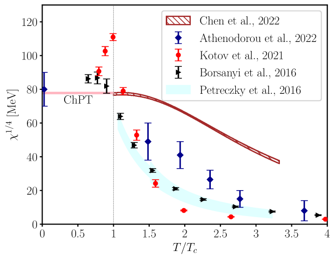
Figure 6.1: Comparison of different determinations of the fourth root of the topological susceptibility $\chi^{1/4}$ in $N_{f}=2+1$ QCD from lattice simulations. Diamond points are taken from [494], round points from Ref. [11], triangle points from Ref. [491] (removing the isospin-breaking factor), the dashed area represents results of Ref. [518], while the shaded area represents results of Ref. [492] obtained from the chiral susceptibility for unphysical pion mass and rescaled according to the DIGA prediction $\chi^{1/4}\sim m_{\pi}$. For the crossover temperature the reference value $T_{c}=155$ MeV is assumed. For comparison we also report results obtained below the crossover, as well as the NLO two-flavor $T=0$ ChPT prediction for degenerate up-down quarks $\chi^{1/4}_{\mathrm{ChPT}}(T=0)=77.8(4)$ MeV.

These recent determinations with $N_{f}=2+1$ flavors are displayed and compared in Fig. 6.1. Roughly speaking, there is qualitatively a general common agreement that, for temperatures $T\gtrsim 300$ MeV (i.e., $T/T_{c}\gtrsim 2$) the behavior of $\chi(T)$ is compatible with a power-law as predicted by the DIGA, with a compatible exponent $\chi^{1/4}(T)\sim(T/T_{c})^{2}$. However, results of Ref. [491] find a very good agreement with the DIGA exponent already soon after the crossover, while Refs. [474, 492, 494] point out a change in the effective exponent for $T/T_{c}\gtrsim 2$.

Since in recent times several works gathered evidence for the existence of a phase of QCD close to the crossover and below $T\approx 300$ MeVs where non-perturbative effects are dominating [27, 519, 520, 521], this aspect surely deserves to be further investigated in the near future, with dedicated studies aiming at addressing the behavior of QCD close to the crossover (see also Ref. [474]). These recent findings also match very well with other lattice studies pointing out the abundance of instanton-dyons in this temperature range above the crossover, see, e.g., Refs. [522, 523, 524].

Nonetheless, we can still fairly conclude that, while the one-instanton semiclassical computation is likely to be not reliable in the range currently reached by lattice simulations (for example, the authors of Ref. [491] find that the DIGA prediction is about one order of magnitude smaller than their lattice determinations), the assumption of non-interacting instantons becomes reasonably reliable when considering temperatures $T\gtrsim 300$ MeV. This is also in agreement with results of Refs. [525, 491, 481, 493], where determinations of the quartic coefficient (related to the quartic axion auto-interaction term)

$$b_{2}\equiv-\frac{1}{12}\frac{\langle Q^{4}\rangle-3\langle Q^{2}\rangle^{2}}{\langle Q^{2}\rangle}$$ (6.14)

for $T/T_{c}\gtrsim 2$ are in very good agreement with the well-known DIGA prediction $b_{2}^{(\mathrm{DIGA})}(T)=-1/12$, which only stems from the assumption of dilute instantons alone, and is unrelated to the semi-classical calculation needed in addition to the latter to compute $\chi_{\mathrm{DIGA}}(T)$ (see also Fig. 7 of Ref. [474] for a comparison of different high-temperature lattice determinations of $b_{2}$ in full QCD).

As for a quantitative agreement on the value of the topological susceptibility, no conclusive consensus on its exact behavior as a function of $T$ from different computations performed with different strategies has been reached yet, as it is manifest from Fig. 6.1. Therefore, the determination of $\chi(T)$ in full QCD from the lattice above the crossover still poses a difficult yet stimulating challenge and certainly deserves to be further investigated in the near future.

However, it is interesting to observe that, although the underlined differences exist, their impact on axion mass windows is not so pronounced. Solving the axion equation of motion in the background of the Friedmann–Lemaître–Robertson–Walker metric, and using the simple DIGA parametrization for the $\theta$-dependence of the QCD free energy

$$f_{\mathrm{DIGA}}(\theta)=A\left(\frac{T}{T_{c}}\right)^{-d}\cos(\theta),$$ (6.15)

it is possible to derive:

$$\frac{\Omega_{\mathrm{A}}}{\Omega_{\mathrm{DM}}}\simeq Cm_{a}^{-\frac{3.053-d/2}{2.027-d/2}},$$ (6.16)

where $\Omega_{\mathrm{A}}$ is the relic axion energy density, $\Omega_{\mathrm{DM}}$ is the observed Dark Matter energy density, and $C$ is a pre-factor depending weakly on the decay constant $d$ and mainly and on the pre-factor $A$ appearing in Eq. (6.15), as well as on the details of the axion model. More details on the derivation of Eq. (6.16) can be found, e.g., in Refs. [474, 505, 11, 526]. Using the parametrization (6.16), it is possible to show that even by changing $d$ by a factor of $2$ or $A$ by four orders of magnitude, the axion mass predictions stay essentially in the same ballpark [474, 505, 11], cf. also Fig. 6.2.

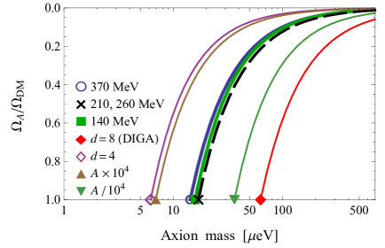
Figure 6.2: Figure taken from Ref. [11]. Dependence of the ratio $\Omega_{\mathrm{A}}/\Omega_{\mathrm{DM}}$ on the axion mass according to Eq. (6.16) for physical [11] and unphysical [505] pion mass ensembles. For the $m_{\pi}\simeq 140~{}\text{MeV}$ ensemble, parameters $A$ and $d$ obtained from the best fit of data of Ref. [11] to Eq. (6.5) are varied as written in the legend.

Nonetheless, further studies to clarify the high-temperature behavior of the QCD topological susceptibility would be welcome, and the current state of the art can be improved in several directions. For instance, it would be interesting to refine existing results closer to the crossover, where non-perturbative effects are more pronounced, and where most of the current tensions take place. It would also be intriguing to probe higher temperatures from lattice simulations, as most of the results obtained so far, with only the exception of Ref. [491], were limited to the $160~{}\text{MeV}\lesssim T\lesssim 600$ MeV range. In particular, it would be extremely interesting to reach temperatures of the order of $\sim 1$ GeV or above (i.e., $T/T_{c}\sim 10$), which is also necessary to study axion cosmology.

However, probing such high temperatures is at present an extremely tough challenge from the numerical point of view, because of the topological freezing problem. At present, several promising proposals have appeared in the literature to deal with the topological slowing down in simpler models. As an example, in Ref. [527], machine-learning techniques via the so-called Equivariant Flows are employed to mitigate freezing in the $2\mathrm{D}$ $\mathrm{U}(1)$ gauge theory and extensions to more complex gauge theories are expected in the near future. Another proposal can be found in Ref. [222] (see also Lucini_talk), a strategy based on the adoption of a parallel tempering scheme on the inverse gauge coupling $\beta$ in combination with the Density of States approach has been adopted in the pure $\mathrm{SU}(3)$ gauge theory to reduce the large auto-correlation times affecting the Monte Carlo evolution of $Q$. We also note the method adopted in Ref. [528] to avoid topological freezing and the dominance of the $Q=0$ sector. That paper presents simulations at a single beta, using density of states as a function of a proxy topological charge. It also uses parallel tempering for the different charge values. Another promising solution is the parallel tempering on boundary conditions proposed by M. Hasenbusch for $2\mathrm{D}$ large-$N$ $\mathrm{CP}^{N-1}$ models [529] and adopted both in the latter case [504, 530] and in $4\mathrm{D}$ large-$N$ $\mathrm{SU}(N)$ pure-gauge theories [531, 532] to mitigate the effects of the topological slowing down by reducing the auto-correlation times of $Q$ by up to several orders of magnitude.

6.3   The Road Ahead

Topology in QCD plays a central role in determining the non-perturbative properties of the theory, and has been further revived by the quest for QCD axions. Further discussions on topology will be included in the contributions to a dedicated series of workshops that are planned to be held in Europe in 2023 and following years. For instance, NA6 participants are involved in the new EU COST “CosmicWISPers”, involving both Claudio Bonanno and Maria Paola Lombardo. Moreover, topology will also be the main topic of the dedicated series of workshops “Gauge Topology”, co-led by Massimo D’Elia, that is held in ECT^⋆ in Trento every two years. Finally, the QCD axion physics will also be covered during the “Lattice Gauge Theory Contributions to New Physics Searches” workshop in Madrid, which includes Claudio Bonanno in the organizing committee. In the near future, we foresee a more robust limit on the QCD axion mass, as well as more in-depth studies of the axion potential. Such studies will also help in clarifying the role of topology in the Quark Gluon Plasma phase (see also the discussion in Sec. 3).

7   Statistical Field Theory

In this section, we discuss three topics that show how strong the connection between Quantum Field Theories and Condensed Matter/Statistical Mechanics Models is. These advanced topics were covered in Pelissetto_talk,Sorba_talk,KitchingMorley_talk. Discussions on applications of universality classes for continuum transitions and conformal theories are in Sections 2, 5.

7.1   Phase Diagram of Three-Dimensional Abelian-Higgs Models

Three-dimensional Abelian gauge theories coupled to scalar matter (Abelian-Higgs models) have recently drawn significant attention, as they arise as low-energy effective field theories describing unconventional states of matter with fractionalized quantum numbers occurring in two-dimensional strongly-correlated quantum systems. They are relevant for superconductors, superfluids, and quantum SU($N$) antiferromagnets [533, 534, 535, 536, 537, 538, 539, 540]. In particular, they are expected to describe the transition between the Néel and the valence-bond-solid state in two-dimensional antiferromagnetic SU(2) quantum systems [541, 542, 543, 544, 545, 546, 547, 548], which represents the paradigmatic model for the so-called deconfined quantum criticality [549]. The behavior in the presence of massless fermionic excitations is also equally relevant in, e.g., high-$T_{c}$ superconductors and spin liquids; see Refs. [550, 551, 552, 553, 554, 555, 556, 557] and references therein.

In the lattice scalar Abelian-Higgs (AH) model the scalar fields are $N$-component vectors $\phi_{x}$ defined on the sites of a lattice. As for the gauge fields, two different formulations are possible. In the noncompact model the gauge field is a real field $A_{{x},\mu}$ defined on the sites of the lattice (for definiteness we consider cubic lattices, so that each link is labelled by a lattice site ${x}$ and a direction $\mu$) and the gauge group is the additive group of the real numbers $\mathbb{R}$. In the compact formulation, the gauge field is a complex phase $U_{{x},\mu}$ and the gauge group is U(1). The action is $S=S_{\phi}+S_{g}$, where the matter-field part is

$$S_{\phi}=-J\sum_{{\bm{x}}\mu}\phi^{*}_{\bm{x}}\cdot\phi_{{\bm{x}}+\hat{\mu}}\,U_{{\bm{x}},\mu}^{Q}+\sum_{{\bm{x}}}V(|\phi_{\bm{x}}|),$$ (7.1)

where $V(x)$ is a generic potential [most of the numerical work considered fixed-length fields, corresponding to $V(x)=\delta(x-1)$]. Here $Q$ is the integer charge of the fields (it is only relevant in the compact case) and $U_{{\bm{x}},\mu}=\exp(iA_{{\bm{x}},\mu})$ in the non-compact case. The gauge action $S_{g}$ is the standard Wilson action in the compact case; otherwise, we set

$$S_{g}=\kappa\sum_{{\bm{x}},\mu>\nu}(\nabla_{\mu}A_{{\bm{x}},\nu}-\nabla_{\nu}A_{{\bm{x}},\mu})^{2},$$ (7.2)

where $\nabla_{\mu}f({\bm{x}})=f({\bm{x}}+\hat{\mu})-f({\bm{x}})$ is the lattice nearest-neighbor derivative. The model is invariant under U(1)/$\mathbb{R}$ local and $SU(N)$ global transformations.

AH models have been extensively studied, see Refs.  [558, 559, 560, 561, 562, 563] and references therein. The phase diagram turns out to depend in a nontrivial fashion on the compact/noncompact nature of the gauge interactions and also the charge of the scalar fields (see Ref. [564] for a discussion of the charge dependence of the phase diagram). Here we will summarize the behavior along two different transition lines where the scalar field condenses and the global $SU(N)$ symmetry of the theory is broken.

For small values of $\kappa$, there is an order-disorder transition at a finite value $J_{c}(\kappa)$ of the scalar coupling $J$. Such a transition is always discontinuous, except for $N=2$. For $N=2$ the transition is continuous, in the O(3) universality class, irrespective of $Q$ and of the nature of the gauge fields. These small-$\kappa$ transitions are an example of Landau-Ginzburg-Wilson (LGW) transitions. In this case, an effective description is obtained by considering a gauge-invariant scalar field $\Psi$ that represents a coarse-grained version of the microscopic order parameter that signals the onset of long-range order. The effective action is then the most general $\Psi^{4}$ theory that is invariant under the global symmetry group of the AH model. At LGW transitions the gauge group and the nature of the gauge fields do not play any role. Gauge invariance is only relevant in defining the set of observables that show a critical behavior.

For large values of $\kappa$, AH systems also undergo an order-disorder transition, but in this case model details are relevant. For the compact model with $Q=1$, the transition has the same nature as for small $\kappa$: it is an LGW transition. On the other hand, in the noncompact case or in the compact case with charge-$Q$ fields, $Q\geq 2$, a critical transition is observed for $N\geq 7(2)$ [561, 562, 563]. This transition is associated with a stable fixed point of the renormalization-group flow of the continuum AH field theory. The fixed point is charged—the renormalized gauge coupling is nonvanishing at the fixed point— signaling that gauge fields play a role in determining the critical behavior.

It is important to extend the present analysis to AH models with fermions, which are relevant to understand the finite-temperature QCD transition. The analysis pioneered by Pisarski and Wilczek [13] effectively assumes that this transition is a LGW one in which only the global symmetry group is relevant. However, we cannot exclude a priori the existence of continuous transitions with critical gauge excitations as it occurs in the scalar AH model for $N\gtrsim 7$. Further work is clearly needed to settle this issue.

7.2   Interfaces Near Criticality: Results from Field Theory

In statistical systems exhibiting a phase transition, the coexistence of different phases at criticality naturally leads to the formation of an interface. On the other hand, in particle physics, the confinement of quarks into hadrons is effectively described in terms of a string spanning an interface over time. Since duality relates a lattice gauge theory to a spin model, the two problems turn out to be deeply connected and both are conveniently addressed using the Ising model as a base system.

We thus consider the three-dimensional Ising model in its broken $\mathbb{Z}_{2}$ symmetry phase below the critical temperature $T_{c}$, where an interface separating coexisting phases of opposite magnetization is easily induced by a suitable choice of the boundary conditions. The linear size $R$ of the interface must be much larger than the correlation length $\xi$, in order that the two distinct phases to emerge over bulk fluctuations. In [565] the phenomenon is studied for a slab geometry of size $L\times L\times R$ (with $L\to\infty$), in which the magnetization tends to the pure values $\pm M$ as $x\to\pm\infty$ hence creating an interface running between the lines $x=0$, $z=\pm R/2$. Conversely, only the half-volume $x\geq 0$ is considered in [566] with the interface pinned along the boundary condition changing lines $z=\pm R/2$ on the impenetrable wall $x=0$. Working in the scaling limit slightly below $T_{c}$, universal properties emerge and both systems are described by a field theory that admits a particle description. As a consequence, the interface is depicted as the propagation of a string of particle modes and this provides insight on the interfacial tension (i.e. the free energy of the interface per unit area), which is found for both geometries to be related to the particle density along the string and to be fully consistent with an independent Monte Carlo estimation provided in [567]. It is then possible to derive analytically the expectation value of any observable with the given boundary conditions $\langle\Phi(x,y,z)\rangle_{\pm}$, using the asymptotic $n$-particle states $|\bf{p}_{1},...,\bf{p}_{n}\rangle$ of the bulk field theory as a basis on which generic excitations can be expanded. More specifically, the configurational averages are expressed in momentum space and the condition $R\gg\xi$ selects the low energy particle modes. The analytic results for the order parameter profile $\langle s(x,y,z)\rangle_{\pm}$ are on one side [565] explicitly confirmed by means of Monte Carlo simulations performed for different values of $R$ and $T\lesssim T_{c}$, in the total absence of adjustable parameters; on the other side [566], they allow for a simple probabilistic interpretation of the interface as a sharp separation between the two phases. Moreover, in the half-volume system [566], the particle formalism explains the transition from a fluctuating to a binding regime of the interface with respect to the wall, when their interaction becomes sufficiently attractive. Thanks to scattering theory, some key parameters characterizing the binding transition are computed and compared with numerical data coming from the phenomenological wetting theory.

As already anticipated, the study of interfaces in spin models can be useful even when dealing with lattice gauge theories. Concerning the three-dimensional Ising model, we know that it is mapped by duality into the three-dimensional Ising gauge model and, for instance, the interface free energy is analogous to the Wilson loop expectation value. We could hence expect our exact formulation of interfaces close to criticality to be valuable also in characterizing observables close to the critical point in the three-dimensional Ising gauge model. Otherwise, an effective description of the interface behavior can be adopted, resulting in capillary wave theory for the spin model and effective string theory for the corresponding lattice gauge model. In particular, the capillary wave model corresponds (see [568, 569] for a discussion of this point) to the well known Nambu-Goto effective string theory [570, 571], which has been shown in the last few years to give a very precise description of Wilson loops thanks to the so-called low energy universality theorem (see [572, 573] for a review).

Finally let us mention that, besides the one discussed above, it is also possible to give a consistent field theoretic description of interfaces with a Landau-Ginzburg type action for the order parameter of the model [574]. In this framework it is possible to obtain analytic expressions for the interface profile and width [574] which are fully consistent with those obtained with the capillary wave model but do not require the ad hoc cut-offs terms which must be introduced in the standard capillary wave model.

7.3   Infrared Finiteness of Three-Dimensional Super-Renormalisable QFTs

Three-dimensional super-renormalizable scalar QFTs with fields in the adjoint representation of the $\operatorname{\mathrm{SU}}(N)$ group attracted lot of interest in the past as effective (dimensionally reduced) theories describing the high-temperature limit of four-dimensional Yang-Mills theories (see, for example, [575, 576, 577, 578, 579, 580]). More recently these theories attracted a renewed interest as candidate holographic models for the very early universe [581].

A relevant open problem in this context is represented by the fact that massless super-renormalisable quantum field theories suffer from severe infrared (IR) divergences in perturbation theory: the same power counting argument that implies good ultraviolet (UV) behavior also implies bad IR behavior. These IR singularities were discussed several years ago in [582, 575] where it was conjectured that such theories are nonperturbatively IR finite. The lattice regularization offers a perfect setting to address this issue, which was recently discussed in [583] in the particular case of scalar QFTs with a $\phi^{4}$ interaction and fields in the adjoint representation of the $\operatorname{\mathrm{SU}}(N)$ group with $N=2,4$.

When studied in lattice perturbation theory, these theories exhibit a logarithmic IR divergence for the critical mass at the two-loop level. However, this divergence was not present in the lattice simulations of [583] thus providing strong evidence for the IR-finiteness of the full theory. From the lattice results it was also possible to obtain a nonperturbative determination of the critical masses which turns out to agree with 2-loop perturbation theory, and a determination of the critical exponent which turns out to be close to the leading-order effective theory prediction [583].

These results open the way to a better understanding of the infrared properties of this class of models which could have remarkable implications both for the high $T$ description of Yang–Mills theories and for candidate holographic models of the early Universe.

7.4   The Road Ahead

The three examples discussed in this section show how powerful the Statistical Field Theory approach can be when combined with simulations. This is particularly true for critical systems and more generally for systems in the neighborhood of a phase transition which are the main focus of this report. Statistical Field Theory allows to propose effective description for the systems of interest (LGW models for the phase diagram of Abelian Higgs models, effective strings for the interfaces, holografic models for the early universe…) which can then be tested and refined with Monte Carlo simulations. With the improvement of computing power and algorithms (see the next section for a discussion of the remarkable performances of new, machine learning based, algorithms), this virtuous circle between effective theories and simulations will lead to more and more refined models also for QCD related phase transitions and, what is more important, to a more precise description of the relevant degrees of freedom in this context.

8   Machine Learning

8.1   Introduction

Recent advances in the implementation of Machine Learning (ML) techniques for physical systems, especially those which can be formulated on lattices, appear to be suitable for observing the corresponding underlying phase structure of the aforementioned systems [584, 585, 586, 587, 588, 589, 590, 591, 592, 593, 594, 595, 596, 597, 598, 599, 600, 601]. This, was firstly observed in the novel work by J. Carrasquilla and R. G. Melko in 2017 [602] where they used supervised machine learning architectures with fully connected and convolutional neural networks to identify phases and phase transitions in a variety of condensed-matter Hamiltonians. For instance, they can estimate to an adequate precision the critical exponents as well as the critical temperature for the 2D ferromagnetic Ising model. The above advance was followed by a plethora of investigations using Principal Component Analysis (PCA) [586, 585, 590, 603, 604], Supervised Machine Learning (ML) [587, 594, 605], Restricted Boltzmann Machines (RBMs) [606, 607], as well as autoencoders [590, 589] which appear to successfully identify different phase regions of classical statistical system. Since Quantum Field Theories can be represented in the form of statistical systems it would be reasonable to expect that such methods could apply in Quantum Field Theories. So far only a few investigations dealt with the phase structure of Quantum Field Theories on the lattice. These works will be reviewed throughout this next chapter.

8.2   Phase Transition Recognition in $\operatorname{\mathrm{SU}}(N)$ Gauge Theories and QCD

The first investigation which has provided a successful identification of the confining-deconfining transition in $SU(2)$ gauge theory using Machine Learning techniques has been reported in Ref. [608]. Namely, the authors using Principal Component Analysis (PCA) on configurations produced for a range of values of $\beta$, demonstrated that even though the $SU(2)$ order parameter Polyakov loop is non-linear, PCA captures indications of a phase transition at the range of $\beta$ $\in$ [1.8, 2.2]. This has been achieved by probing the “average mean squared error reconstruction loss” as well as the “average norm of the PC”. Surprisingly, at the same time they demonstrated that there is no correlation between the Polyakov loop and the principal components. The above is demonstrated in Fig. 8.1. Bear in mind that $SU(2)$ link matrices can be mapped to four real numbers multiplying the $3$ Pauli matrices and the unity.

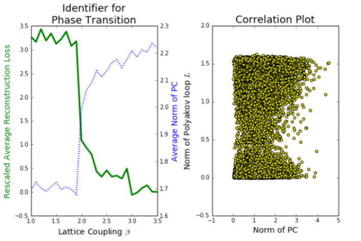
Figure 8.1: (Ref. [608]) Finding a possible phase transition with PCA. Left Panel: The average mean squared error reconstruction loss as a function of temperature is a universal identifier for a phase transition. This was calculated in 100 independent PCA runs with two principal components (PC), measured in units of $\times 10^{-5}$ and shifted by the value at $\beta=3.5$. The average norm of the PC also indicates a phase transition. Right Panel: A plot indicating that there is no correlation between the principal components and the Polyakov loop.

Subsequently, the authors turned to the investigation of the phase structure using the Correlation Probing Neural Network. The Correlation Probing Neural Network consists of three types of neural networks stacked on top of each other. The localization network is a fully convolutional neural network which prohibits connections outside of the receptive field of each output neuron. The averaging layer averages over the input from the localization network. The prediction network is a fully connected neural network, which transforms the output of the averaging layer to a prediction probability. The authors trained the correlation probing neural network in a supervised manner on $SU(2)$ Monte Carlo-sampled configurations at lattice couplings $\beta$ $\in$ [1, 1.2] in the deconfining phase and $\beta$ $\in$ [3.3, 3.5] in the confining phase. Then, they tested the neural network for values of lattice coupling $\beta$ $\in$ [1.3, 3.2] and they predicted a phase transition at $\beta=1.99\pm 0.10$ for lattice of $T\times L_{x}\times L_{y}\times L_{z}=2\times 1\times 1\times 1$ and $\beta=1.97\pm 0.10$ for a lattice of $2\times 8\times 8\times 8$ while a conventional lattice calculation gives a critical value of $\beta=1.880\pm 0.025$. This result has been obtained by probing the average prediction probability.

Finally, the authors move to the more conclusive part of their investigation where they trained a new neural network on the local data samples in order to classify the phases of each local sample. This enables the local neural network to associate a prediction to each patch. The authors performed polynomial regression on the latent prediction of the local neural network. By extracting the weights of the regression they demonstrated that the parameter which quantifies the phase transition is nothing else but the Polyakov loop on a single spatial lattice site! Subsequently, by acting on the full lattice the decision function takes the form of the Polyakov loop as the argument on a Sigmoid function on the full lattice. This is clear evidence that supervised machine learning can predict the correct order parameter of the theory.

The work of Ref. [608] was followed by the investigation of the phase structure of $SU(2)$ and $SU(3)$ in Ref. [609]. The authors have developed a supervised Machine Learning network capable of identifying the order parameter of the theory, namely the Polyakov loop. The architecture of the neural network they used can be summarised in the next couple of lines. $SU(2)$ is parametrized by four real numbers while for $SU(3)$ the authors used the full set of 9 complex numbers. Consider a gauge field with $\left[N_{t},N_{s},N_{s},N_{s},{\rm Dim},{\vec{v}}_{\rm SU(N)}\right]$, where $N_{t}$, $N_{s}=N_{x}=N_{y}=N_{z}$ the temporal and spatial lattice extents, Dim the direction $\mu$ of the matrix $U_{\mu}(x)$ at every lattice site $[N_{t},N_{s},N_{s},N_{s}]$ and ${\vec{v}}_{\rm SU(N)}$ the vector of the representation with size 4 and 9 for $SU(2)$ and $SU(3)$ respectively. The architecture of the neural network for the prediction of the Polyakov loop in the $\operatorname{\mathrm{SU}}(N)$ gauge theory is expressed as first for $N_{t}=2$: Inputlayer: $(N_{t},N_{s}\times N_{s},N_{s},{\rm Dim}\texttimes U)$ $\to$ Convolutional3D $(N_{t},N_{s}\times N_{s},N_{s},{\rm Dim}\texttimes U)$ $\to$ AveragePooling3D $(N_{t},N_{s}\times N_{s},N_{s},16)$ $\to$ Flatten $(1,1,1,16)$ $\to$ Dense $(16)$ $\to$ 1 while for $N_{t}=4$: Inputlayer: $(N_{t},N_{s}\times N_{s},N_{s},{\rm Dim}\texttimes U)$ $\to$ Convolutional3D $(N_{t},N_{s}\times N_{s},N_{s},{\rm Dim}\texttimes U)$ $\to$ Convolutional3D $(2,N_{s}\times N_{s},N_{s},256)$ $\to$ AveragePooling3D $(1,1,1,32)$ $\to$ Flatten $(1,1,1,16)$ $\to$ Dense $(32)$ $\to$ 1.

For training purposes, the authors generated 9000 lattice configurations at the one value of $\beta$ of the lattice coupling, $\beta=4$ for $SU(2)$ and $\beta=10$ for $SU(3)$, for lattices with the spatial sizes $N_{s}=8,16,32$ and the temporal sizes $N_{t}=2,4$. In addition for prediction purposes, they also generated 100 configurations for a number of points at lower values of the coupling $\beta$, which the neural network does not use for training but rather for prediction.

The network is being trained on the lattice configurations generated in the (volume-induced) deconfinement phase at a point of $\beta$ which is far from the phase transition point. The neural network is trained to predict correctly the value of the Polyakov loop that is already known from the Monte Carlo simulations. The training is done in batches of 10 - 50 configurations. The authors used the mean squared error (MSE) as a loss function.

The overall findings resulted out of this investigation demonstrate that the neural network which was trained on a value of $\beta$ located deep in the deconfinement region reproduces the Polyakov loop with an adequate agreement with Monte-Carlo data at all other values of the lattice coupling constant including the region of the true deconfinement transition. This can be viewed in Fig. 8.2 where results for $SU(3)$ at $N_{t}=2$ are presented. These data illustrate the agreement between the Polyakov loop and its approximation using Machine Learning. Hence, what the authors demonstrated is that the neural network serves as a successful predictor of the confining-deconfining phase transition obtained by reconstructing the gauge-invariant order parameter in the whole physical region of the $\beta$-parameter space after one performs training on lattice configurations at one unphysical point in this space. It would have been useful to extend this work from the second order phase structure of $SU(2)$ and the weakly first order phase structure of $SU(3)$ to $SU(N>3)$ where the phase structure is strongly first order.

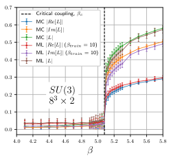
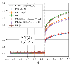
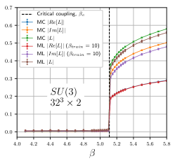
Figure 8.2: (Ref. [609]) The results for the Polyakov loop for SU(3) gauge theory at $N_{t}=2$ obtained with the Monte Carlo simulations as compared to the neural network prediction. The absolute value, the real and imaginary parts of the loop are shown. The value of the Machine Learning extracted approximation of Polyakov loops $ML\ |L|$ restored from ML predictions of $|Re[L]|$ and $|Im[L]|$ are also presented.

Recently, the authors of the Lattice 2021 Proceedings [610] published results on the investigation of the critical temperature on pure $SU(3)$ gauge theory as well as in $N_{f}=2+1+1$ QCD using Machine Learning techniques.

Instead of probing the actual $SU(3)$ configurations which can be reduced down to eight real numbers, per lattice point, and per Euclidean direction, the authors extracted the temporal Polyakov loop for each time slice. The above set-up corresponds effectively to a 3-dimensional system where the basic degrees of freedom are the values of the Polyakov loop at each point of the effective 3D grid.

To classify configurations of Polyakov loops at different temperatures, the authors built a $3D$-convolutional autoencoder using TensorFlow [611] and Keras [612]. The autoencoder is trained, as a whole, to reproduce as output its own input. When this is achieved, the encoded classifier effectively encodes the most important feature(s) describing the variety of the input. The authors simplified the process, by performing a semi-supervised training by pinning some of the input configurations at extreme temperatures to predefined values of the encoded classifier.

For the pure $SU(3)$ gauge theory the authors used configurations of size $T\times N_{x}\times N_{y}\times N_{z}=4\times 8\times 8\times 8$ produced using the MILC code. For this choice of geometry and action, the pseudocritical coupling is $\beta_{C}=5.69(2)$ giving a critical temperature of $T_{C}\sim$ 260 MeV. The authors analyzed 30 configurations for each temperature. The configurations span a wide range of the coupling parameter $\beta$ from strong to very weak coupling. By training the autoencoder as an unsupervised and semi-supervised classification problem the authors obtained an encoded classifier clearly related to the order parameter which in this case is the Polyakov loop. As a matter of fact, two phase sectors are identified by the encoded classifier, one below $T_{C}$ and one above. Namely, above $T_{C}$ the unsupervised scheme highlights the $Z_{3}$ symmetry breaking with three different values of the encoded classifier being equally probable while below $T_{c}$ there is only one possibility with the encoded classifier being zero. When it comes to the semi-supervised learning problem, the authors pinned a fraction of $\sim 20\%$ of the training configurations at the lowest and highest values of $T$ by assigning an encoded classifier of $0$ and $1$ for confining and de-confining phase respectively. The network appears to successfully recognize the phase transition at $T\simeq T_{C}$.

Regarding full QCD with $N_{f}=2+1+1$ fermions, the configurations have been produced with Wilson fermions at maximal twist on a lattice of $32^{3}$ spatial volume with the strange and charm masses having their physical values while the pion mass being $M_{\rm\pi}\sim 370$ MeV. The pseudocritical temperature is $M_{\rm\pi}\sim 200$ MeV. For each temperature, the authors used 200 Polyakov loops configurations. For the case of QCD, the Polyakov loop is no longer an order parameter and the identification of a phase transition based on the Polyakov loop is not theoretically justified as before. The authors studied the semi-supervised problem by assigning to the configurations at low temperatures an encoded classifier of 1 and at higher temperatures of 0. The resulting encoded classifier turns out to be a much smoother function compared to the one for the pure gauge theory. This is somehow expected since the phase transition for the QCD configurations is known to be a crossover. From the encoded classifier the authors could identify two classes separated at temperature $T\sim 1.5T_{C}$.

The authors have successfully used the Convolutional neural networks trained as either unsupervised or semi-supervised classifiers to identify different phases of gauge theories in both pure gauge as well as full QCD. Further work needs to be carried out, namely by moving to a finer temperature scan, a finite-size scaling and a continuum limit. This will improve the performance of the autoencoder. Finally, this will hopefully provide further insight into Machine-Learning approaches to the study of phase transitions.

Recently, in Ref. [41] the authors used Normalizing Flows instead of the traditional rewriting in $\beta$ in order to interpolate the chiral condensate obtained from QCD simulations with five degenerate quarks. Namely, the authors performed calculations in five-flavor QCD $(N_{f}=5)$ using the HISQ action with quark masses in the range $0.001\leq m_{l}\leq 0.016$ and gauge couplings $\beta=4.5-5.4$. They used 4-dimensional lattices with volume $N_{s}^{3}N_{t}$, with temporal extent $N_{t}=6$ and spatial volumes $N_{s}^{3}=16^{3},24^{3}$. Subsequently, they performed the classical reweighing in $\beta$ to provide an interpolation of the chiral condensate in $\beta$.

Lattice QCD calculations typically are done at a few values of the gauge coupling beta and reweighting in beta is a popular method for interpolating lattice results. This method requires a large number of measurements, performed at a large number of beta values since the observable we are interested in is extracted via the 2D histogram of the action and the observable. As explained before the observable under investigation is the chiral condensate and the interpolation is done in the direction of beta. Applying reweighting reveals reasonable results for small masses $(0.002\leq m_{l}\leq 0.005)$, but exhibits over-fitting for larger values of masses $(m_{l}=0.006,0.008)$.

Followingly, authors turned to normalizing flows which are state-of-the-art ML tools for modeling probability distributions in physical systems. They made use of MAF (Masked Autoregressive Flow) [613] model with eight MADE (Masked Autoencoder for Distribution Estimation) [614] blocks. Compared to classical reweighting, this method has the advantage of allowing to interpolate in any parameter. As a matter of fact, in this process there is no need for overlapping distributions of the action density and the method is able to process continuous data. The cost to pay in order to visualize the learned probability distribution is the fact that one needs to draw a large number of samples from the model to fill a two-dimensional histogram. In practice, the model learns to transform a 2D-Gaussian distribution to expectations of the chiral condensate and action $({\bar{\psi}}\psi,S)$ conditioned on the parameters ($N_{s}$, $m_{l}$, $\beta$). The evaluation of the model was performed for All the integer values of $N_{s}\in[16,24]$, $\beta\in[4.5,5.4]$ in steps of $0.001$ and $m_{l}\in[0.001,0.006]$ in steps of 0.001 and for the larger masses $m_{l}\in[0.008,0.016]$ in steps of 0.002. This allowed the authors to fit the entire data set with a single function $p({\bar{\psi}}\psi,S|N_{s},m_{l},\beta)$ in contrast to the $\beta$-reweighting according to which one needs to do independent reweighting for each mass and volume. A comparison to the reweighting method reveals that the normalizing flow results appear to give a better fit since now the data points support each other also in $m_{l}$ and $N_{s}$-directions and not just in $\beta$. As a result, the method of normalizing flows removes over-fitting appearing in the traditional $\beta$-reweighting.

A glimpse at the 2D histogram in the ${\bar{\psi}}\psi-S$ plane as well as at the 1D histogram in ${\bar{\psi}}\psi$ reveal two phases in the small quark mass regime while only one at the large mass regime which manifests as two and one peaks respectively. The double peaks signal the occurrence of a first order phase transition. To determine the quark mass dependence of the double peaks the authors turned to the phase diagram $\langle{\bar{\psi}}\psi\rangle$ in the $m_{l}$-$\beta$ plane. This enabled them to demonstrate evidence that the first order region ends in a second order endpoint at about $m_{l}^{c}\simeq 0.0045$. As the gap between the peaks at low and high values $\beta$ becomes smaller, larger lattices will be needed to resolve these two peaks and establish a gap between them. To locate the endpoint the authors used another ML based approach called the EOS-meter.

According to the Equation-of-State (EOS) meter, one can use convolutional neural network model to create density plots [615]. The authors used a recent approach called the transformer model [616], which is solely based on attention mechanisms and has been shown to outperform convolutional neural networks in translation tasks. The density plots revealed, at the smallest masses, a two peak behavior with a clear gap which is characterized as “first-order” while in the largest masses one peak behavior has been spotted characterized as “crossover”. “Firstorderness” and “crossoverness” were implemented as categories in one-hot-encoding. The resulting EOS-meter shows that the critical masses marking the borders between first order and crossover regions, extracted via logistic fits to the “firstorderness”, indicate a critical mass at $m_{c}\simeq 0.005(1)$.

As a further investigation, one should move to the extraction of the phase diagram of QCD with $N_{f}$ flavors in the continuum. For this purpose, one should use larger values of $N_{t}$. One can also extend the set of interpolating parameters to $(N_{f},N_{s},N_{t},m_{l},\beta)$, however, this would require a large amount of training data.

8.3   Phase Transition Recognition in Other Theories

We now turn to additional investigations which are focussing mostly on simpler theories such as the $\phi^{4}$ scalar field theory as well as the Ising model.

First, we present the work of Refs. Aarts_talk and [617], where the authors discussed the adoption of Euclidean quantum field theories in machine learning algorithms, which makes inference and learning possible using quantum field dynamics. To do so, it was first demonstrated that the $\phi^{4}$ scalar field theory satisfies the Hammersley–Clifford theorem. As a result, the quantum field theory can be recast as a machine learning algorithm within the mathematically rigorous framework of Markov random fields. Various applications are then possible. For a fixed target distribution, the parameters of the best approximating $\phi^{4}$ model are obtained by minimizing the Kullbach–Leibler divergence (which is an asymmetric distance) between the two. In practical applications, the effectiveness of the minimization is an indicator of the goodness of the approximation. Through re-weighting, the analysis can be extended to complex-valued actions with longer-range interactions. Moreover, neural network architectures derived from the $\phi^{4}$ theory can be viewed as generalizations of conventional neural networks. It is noted that the aims of this work are two-fold: the approach can provide a new perspective on machine learning with continuous degrees of freedom using the language of quantum fields, while also providing a new look at quantum fields when employed as building blocks in neural networks.

Subsequently, we present the work of Refs. Athenodorou_talk and [618] which discusses deep learning autoencoders for the unsupervised recognition of phase transitions in physical systems formulated on a lattice. Their work elaborates on the applicability and limitations of this deep learning model in terms of extracting the relevant physics. Their results are presented in the context of $2D$, $3D$, and $4D$ Ising models as well as the $XY$ model, and the focus is on the analysis of the critical quantities at $2D$ (anti)ferromagnetic Ising Model. The authors defined it as a quasi-order parameter, the absolute average latent variable, which enabled them to predict the critical temperature to adequate precision. In this way one can define a latent susceptibility from the latent variable and use it to quantify the value of the critical temperature $T_{c}(1/L)$ at different lattice sizes and that these values suffer from smaller finite scaling effects compared to what one obtains from the magnetic susceptibility. This feature is demonstrated in Fig. 8.3 where the critical temperature extracted from the magnetic as well as the latent susceptibilities are extrapolated to the thermodynamic limit both converging to Onsager’s solution. Clearly, $T_{c}(1/L)$ extracted using latent susceptibility converges much faster to the theoretical prediction as a result of the smaller finite volume effects. Hence, the deep learning autoencoder could potentially provide a tool that can enable the extraction of physical parameters with much better accuracy that the traditional ways.

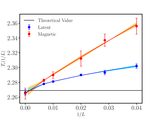
Figure 8.3: Ref. [618] The critical temperature $T_{c}(L)$ for the 2D Ferromagnetic Ising model, extracted from fitting the magnetic (red) and the latent (blue) susceptibilities as a function of $1/L$ according to $T_{c}(L)-T_{c}(L=\infty)\propto L^{-1/\nu}$. The error bands are estimated using the jackknife fit errors on the fit parameters.

Finally, we briefly present the work which can be found in Bachtis_talk. This project demonstrates that the combination of renormalization group methods and machine learning algorithms opens up the opportunity to overcome fundamental problems in computational studies of phase transitions, such as the critical slowing-down effect. In this work, the authors discuss applications of machine learning for phase transitions and present a construction of inverse renormalization group transformations that enables the generation of configurations for increasing lattice volumes in the absence of the critical slowing-down effect. Results are presented for the two-dimensional Ising model and the $\phi^{4}$ theory.

Specifically, the authors demonstrate that the inclusion of a neural network function within the Hamiltonian of the two-dimensional Ising model is able to induce a phase transition by breaking or restoring its symmetry [619]. Another topic of discussion concerns the implementation of a machine learning approach, based on a set of transposed convolutions, to invert a standard renormalization group transformation in the case of the $\phi^{4}$ theory [620]. The inverse transformations are then applied consecutively to iteratively increase the volume of the system, without experiencing the critical slowing-down effect. Both methods result in accurate calculations of multiple critical exponents for the aforementioned systems using renormalization group techniques based on matching observables on lattices of different sizes. These methodological advances rely on the observation that machine learning quantities can be interpreted as statistical-mechanical observables. Consequently, the opportunity to apply histogram reweighting to extrapolate them in parameter space is additionally explored [621]. Finally, an application of a machine learning technique called transfer learning is discussed, which indicates similarities in order-disorder phase transitions [622]. These similarities extend beyond the notions of symmetry and dimensionality which generally characterize the concept of universality.

8.4   The Road Ahead

In summary, machine learning implementations, when combined with renormalization group approaches, are capable of providing significant computational benefits and novel physical insights into studies of phase transitions. These include the evasion of the critical slowing down effect with the inverse renormalization group, and the inclusion of neural networks within Hamiltonians to induce symmetry-breaking phase transitions in systems. As a result, one envisages the benefits of extending the methods discussed here to more complicated and physically relevant systems, such as lattice gauge theories.

A future workshop Machine Learning approaches in Lattice QCD - An interdisciplinary exchange  organized by Nora Brambilla and others at the Institute for Advanced Study of the Technische Universität München will further investigate this topic. The work Density of States approach conducted by Biagio Lucini in Lucini_talk should also be further discussed. For a recent flow-based density of states application to complex actions see [623].

9   Parting Remarks

We have inserted a few comments at the end of each Section, and we would not reiterate them here.

We just summarize that this work highlights, and motivates further, interactions with experimentalists and phenomenologists active in relativistic heavy ion collisions; and with the nuclear astrophysics community, towards the calculation of the equation of state of dense matter and its impact on gravitational waves analysis. Away from these core hadron physics fields, relevant directions include physics beyond the standard model, in particular those aspects related to a strongly coupled Higgs Sector, and the broad field of axions and dark matter. The methodological obstacles related to the sign problem would clearly benefit from closer exchanges with mathematicians and computer scientists.

From the point of view of computational techniques, it is worth remarking that new developments in the rapidly expanding field of quantum computing could lead to major scientific breakthroughs in the coming decades. As already envisioned by Richard P. Feynman in his 1982 work [624] and remarked in Ref. Wiese_talk (see also Ref. [225]), the use of intrinsically quantum computing devices to simulate the quantum field theories describing the elementary constituents of the physical world could have disruptive scientific potential. In particular, it may open the path to solving some of the most challenging problems, including the study of real-time dynamics of strongly coupled theories, the derivation of the properties of systems at finite fermionic densities, and the strong $\mathrm{CP}$ problem.

More generally, the computational aspects remain of crucial relevance for the research topics covered in this review, at the time of the transition between PRACE and EuroHPC [625], and the progress towards Exascale computing Ryan_talk. These issues are also relevant for Open Science policies in the LFT community [626],

The lattice community may provide crucial input to this discussion, and in return greatly benefit from the new developments.

Author contributions

The manuscript has been elaborated and discussed with the authors. The main responsibilities are enlisted below, and specific contributions are indicated as footnotes in the text.

Report coordinators Claudio Bonanno, Michele Caselle, Leonardo Cosmai, Massimo D’Elia, Francesco Di Renzo, Maria Paola Lombardo, Marco Panero.

Editors

• Sec. 1, Maria Paola Lombardo

• Sec. 2, Sipaz Sharma

• Sec. 3, Jana N. Guenther

• Sec. 4, Chris Allton, Christian Schmidt

• Sec. 5, Marco Panero

• Sec. 6, Claudio Bonanno

• Sec. 28, Michele Caselle

• Sec. 8, Andreas Athenodorou

References

- [1] C. Gattringer, C. B. Lang, Quantum Chromodynamics on the Lattice - An Introductory Presentation, Vol. 788, Springer, Berlin, 2010. doi:10.1007/978-3-642-01850-3.
- [2] O. Philipsen, Lattice Constraints on the QCD Chiral Phase Transition at Finite Temperature and Baryon Density, Symmetry 13 (11) (2021) 2079. arXiv:2111.03590, doi:10.3390/sym13112079.
- [3] J. N. Guenther, Overview of the QCD phase diagram: Recent progress from the lattice, Eur. Phys. J. A 57 (4) (2021) 136. arXiv:2010.15503, doi:10.1140/epja/s10050-021-00354-6.
- [4] C. S. Fischer, QCD at finite temperature and chemical potential from Dyson–Schwinger equations, Prog. Part. Nucl. Phys. 105 (2019) 1–60. arXiv:1810.12938, doi:10.1016/j.ppnp.2019.01.002.
- [5] N. Dupuis, L. Canet, A. Eichhorn, W. Metzner, J. M. Pawlowski, M. Tissier, N. Wschebor, The nonperturbative functional renormalization group and its applications, Phys. Rept. 910 (2021) 1–114. arXiv:2006.04853, doi:10.1016/j.physrep.2021.01.001.
- [6] W.-j. Fu, QCD at finite temperature and density within the fRG approach: an overview, Commun. Theor. Phys. 74 (9) (2022) 097304. arXiv:2205.00468, doi:10.1088/1572-9494/ac86be.
- [7] F. Karsch, Critical behavior and net-charge fluctuations from lattice QCD, PoS CORFU2018 (2019) 163. arXiv:1905.03936, doi:10.22323/1.347.0163.
- [8] A. Bazavov, et al., Chiral crossover in QCD at zero and non-zero chemical potentials, Phys. Lett. B 795 (2019) 15–21. arXiv:1812.08235, doi:10.1016/j.physletb.2019.05.013.
- [9] S. Borsányi, Z. Fodor, J. N. Guenther, R. Kara, S. D. Katz, P. Parotto, A. Pásztor, C. Ratti, K. K. Szabó, QCD Crossover at Finite Chemical Potential from Lattice Simulations, Phys. Rev. Lett. 125 (5) (2020) 052001. arXiv:2002.02821, doi:10.1103/PhysRevLett.125.052001.
- [10] H. T. Ding, et al., Chiral Phase Transition Temperature in ( 2+1 )-Flavor QCD, Phys. Rev. Lett. 123 (6) (2019) 062002. arXiv:1903.04801, doi:10.1103/PhysRevLett.123.062002.
- [11] A. Y. Kotov, A. Trunin, M. P. Lombardo, QCD topology and axion’s properties from Wilson twisted mass lattice simulations, PoS LATTICE2021 (2022) 032. arXiv:2111.15421, doi:10.22323/1.396.0032.
- [12] A. Y. Kotov, M. P. Lombardo, A. Trunin, Finite temperature QCD phase transition and its scaling window from Wilson twisted mass fermions, EPJ Web Conf. 258 (2022) 05012. doi:10.1051/epjconf/202225805012.
- [13] R. D. Pisarski, F. Wilczek, Remarks on the Chiral Phase Transition in Chromodynamics, Phys. Rev. D 29 (1984) 338–341. doi:10.1103/PhysRevD.29.338.
- [14] K. Rajagopal, F. Wilczek, Static and dynamic critical phenomena at a second order QCD phase transition, Nucl. Phys. B 399 (1993) 395–425. arXiv:hep-ph/9210253, doi:10.1016/0550-3213(93)90502-G.
- [15] K. Rajagopal, F. Wilczek, The Condensed matter physics of QCD, World Scientific, 2000. arXiv:hep-ph/0011333, doi:10.1142/9789812810458{$\_$}0043.
- [16] A. Butti, A. Pelissetto, E. Vicari, On the nature of the finite temperature transition in QCD, JHEP 08 (2003) 029. arXiv:hep-ph/0307036, doi:10.1088/1126-6708/2003/08/029.
- [17] A. Pelissetto, E. Vicari, Relevance of the axial anomaly at the finite-temperature chiral transition in QCD, Phys. Rev. D 88 (10) (2013) 105018. arXiv:1309.5446, doi:10.1103/PhysRevD.88.105018.
- [18] Y. Nakayama, T. Ohtsuki, Bootstrapping phase transitions in QCD and frustrated spin systems, Phys. Rev. D 91 (2) (2015) 021901. arXiv:1407.6195, doi:10.1103/PhysRevD.91.021901.
- [19] S. Resch, F. Rennecke, B.-J. Schaefer, Mass sensitivity of the three-flavor chiral phase transition, Phys. Rev. D 99 (7) (2019) 076005. arXiv:1712.07961, doi:10.1103/PhysRevD.99.076005.
- [20] O. Kaczmarek, L. Mazur, S. Sharma, Eigenvalue spectra of QCD and the fate of breaking towards the chiral limit (2 2021). arXiv:2102.06136.
- [21] O. Kaczmarek, R. Shanker, S. Sharma, Eigenvalues of QCD Dirac matrix with improved staggered quarks in the continuum limit (1 2023). arXiv:2301.11610.
- [22] P. Lowdon, O. Philipsen, Non-perturbative insights into the spectral properties of QCD at finite temperature, in: 15th Conference on Quark Confinement and the Hadron Spectrum, 2022. arXiv:2211.12073.
- [23] J.-I. Skullerud, et al., Hadrons at high temperature: an update from the FASTSUM collaboration, in: 15th Conference on Quark Confinement and the Hadron Spectrum, 2022. arXiv:2211.13717.
- [24] M. Dalla Brida, L. Giusti, T. Harris, D. Laudicina, M. Pepe, Non-perturbative thermal QCD at all temperatures: the case of mesonic screening masses, JHEP 04 (2022) 034. arXiv:2112.05427, doi:10.1007/JHEP04(2022)034.
- [25] C. Rohrhofer, Y. Aoki, G. Cossu, H. Fukaya, C. Gattringer, L. Y. Glozman, S. Hashimoto, C. B. Lang, S. Prelovsek, Symmetries of spatial meson correlators in high temperature QCD, Phys. Rev. D 100 (1) (2019) 014502. arXiv:1902.03191, doi:10.1103/PhysRevD.100.014502.
- [26] O. Philipsen, L. Y. Glozman, P. Lowdon, R. D. Pisarski, On chiral spin symmetry and the QCD phase diagram, in: 39th International Symposium on Lattice Field Theory, 2022. arXiv:2211.11628.
- [27] A. Alexandru, I. Horváth, Possible New Phase of Thermal QCD, Phys. Rev. D 100 (9) (2019) 094507. arXiv:1906.08047, doi:10.1103/PhysRevD.100.094507.
- [28] V. G. Bornyakov, I. Kudrov, R. N. Rogalyov, Decomposition of the SU(2) gauge field in the maximal Abelian gauge, Phys. Rev. D 105 (5) (2022) 054519. arXiv:2101.04196, doi:10.1103/PhysRevD.105.054519.
- [29] M. Baker, V. Chelnokov, L. Cosmai, F. Cuteri, A. Papa, Unveiling confinement in pure gauge SU(3): flux tubes, fields, and magnetic currents, Eur. Phys. J. C 82 (10) (2022) 937. arXiv:2207.08797, doi:10.1140/epjc/s10052-022-10848-2.
- [30] D. A. Clarke, O. Kaczmarek, F. Karsch, A. Lahiri, M. Sarkar, Sensitivity of the Polyakov loop and related observables to chiral symmetry restoration (8 2020). arXiv:2008.11678.
- [31] J. Braun, B. Klein, Finite-Size Scaling behavior in the O(4)-Model, Eur. Phys. J. C 63 (2009) 443–460. arXiv:0810.0857, doi:10.1140/epjc/s10052-009-1098-8.
- [32] J. Braun, B. Klein, P. Piasecki, On the scaling behavior of the chiral phase transition in QCD in finite and infinite volume, Eur. Phys. J. C 71 (2011) 1576. arXiv:1008.2155, doi:10.1140/epjc/s10052-011-1576-7.
- [33] B. Klein, Modeling Finite-Volume Effects and Chiral Symmetry Breaking in Two-Flavor QCD Thermodynamics, Phys. Rept. 707-708 (2017) 1–51. arXiv:1710.05357, doi:10.1016/j.physrep.2017.09.002.
- [34] J. Braun, W.-j. Fu, J. M. Pawlowski, F. Rennecke, D. Rosenblüh, S. Yin, Chiral susceptibility in ( 2+1 )-flavor QCD, Phys. Rev. D 102 (5) (2020) 056010. arXiv:2003.13112, doi:10.1103/PhysRevD.102.056010.
- [35] F. Gao, J. M. Pawlowski, Phase structure of (2+1)-flavor QCD and the magnetic equation of state, Phys. Rev. D 105 (9) (2022) 094020. arXiv:2112.01395, doi:10.1103/PhysRevD.105.094020.
-
[36]
F. R. Brown, F. P. Butler, H. Chen, N. H. Christ, Z. Dong, W. Schaffer, L. I.
Unger, A. Vaccarino,
On the existence
of a phase transition for qcd with three light quarks, Phys. Rev. Lett. 65
(1990) 2491–2494.
doi:10.1103/PhysRevLett.65.2491.
URL https://link.aps.org/doi/10.1103/PhysRevLett.65.2491 - [37] F. Cuteri, O. Philipsen, A. Sciarra, On the order of the QCD chiral phase transition for different numbers of quark flavours, JHEP 11 (2021) 141. arXiv:2107.12739, doi:10.1007/JHEP11(2021)141.
- [38] Y. Kuramashi, Y. Nakamura, H. Ohno, S. Takeda, Nature of the phase transition for finite temperature QCD with nonperturbatively O() improved Wilson fermions at , Phys. Rev. D 101 (5) (2020) 054509. arXiv:2001.04398, doi:10.1103/PhysRevD.101.054509.
- [39] L. Dini, P. Hegde, F. Karsch, A. Lahiri, C. Schmidt, S. Sharma, Chiral phase transition in three-flavor QCD from lattice QCD, Phys. Rev. D 105 (3) (2022) 034510. arXiv:2111.12599, doi:10.1103/PhysRevD.105.034510.
- [40] Y. Zhang, Y. Aoki, S. Hashimoto, I. Kanamori, T. Kaneko, Y. Nakamura, Finite temperature QCD phase transition with 3 flavors of Möbius domain wall fermions, 2022. arXiv:2212.10021.
- [41] F. Karsch, A. Lahiri, M. Neumann, C. Schmidt, A machine learning approach to the classification of phase transitions in many flavor QCD, in: 39th International Symposium on Lattice Field Theory, 2022. arXiv:2211.16232.
- [42] G. Fejos, Second-order chiral phase transition in three-flavor quantum chromodynamics?, Phys. Rev. D 105 (7) (2022) L071506. arXiv:2201.07909, doi:10.1103/PhysRevD.105.L071506.
- [43] S. R. Kousvos, A. Stergiou, CFTs with Global Symmetry in 3D and the Chiral Phase Transition of QCD (9 2022). arXiv:2209.02837.
- [44] G. Cacciapaglia, C. Pica, F. Sannino, Fundamental Composite Dynamics: A Review, Phys. Rept. 877 (2020) 1–70. arXiv:2002.04914, doi:10.1016/j.physrep.2020.07.002.
- [45] A. Y. Kotov, M. P. Lombardo, A. Trunin, Gliding Down the QCD Transition Line, from = 2 till the Onset of Conformality, Symmetry 13 (10) (2021) 1833. arXiv:2111.00569, doi:10.3390/sym13101833.
- [46] J. Braun, C. S. Fischer, H. Gies, Beyond Miransky Scaling, Phys. Rev. D 84 (2011) 034045. arXiv:1012.4279, doi:10.1103/PhysRevD.84.034045.
- [47] A. Pelissetto, A. Tripodo, E. Vicari, Landau-Ginzburg-Wilson approach to critical phenomena in the presence of gauge symmetries, Phys. Rev. D 96 (3) (2017) 034505. arXiv:1706.04365, doi:10.1103/PhysRevD.96.034505.
- [48] M. Moshe, J. Zinn-Justin, Quantum field theory in the large N limit: A Review, Phys. Rept. 385 (2003) 69–228. arXiv:hep-th/0306133, doi:10.1016/S0370-1573(03)00263-1.
- [49] T. Schäfer, E. V. Shuryak, Phases of QCD at high baryon density, Lect. Notes Phys. 578 (2001) 203–217. arXiv:nucl-th/0010049.
- [50] D. Blaschke, K. Redlich, C. Sasaki, L. Turko (Eds.), Understanding the Origin of Matter: Perspectives in Quantum Chromodynamics, Vol. 999, 2022. doi:10.1007/978-3-030-95491-8.
- [51] C. Sasaki, Signatures of chiral symmetry restoration in dilepton production, Phys. Lett. B 801 (2020) 135172. arXiv:1906.05077, doi:10.1016/j.physletb.2019.135172.
- [52] M. Marczenko, K. Redlich, C. Sasaki, Chiral symmetry restoration and matter formation in neutron stars, Phys. Rev. D 105 (10) (2022) 103009. arXiv:2203.00269, doi:10.1103/PhysRevD.105.103009.
- [53] C. Sasaki, Anomaly-induced chiral mixing in cold and dense matter, Phys. Rev. D 106 (5) (2022) 054034. arXiv:2207.00274, doi:10.1103/PhysRevD.106.054034.
- [54] M. G. Alford, A. Kapustin, F. Wilczek, Imaginary chemical potential and finite fermion density on the lattice, Phys. Rev. D 59 (1999) 054502. arXiv:hep-lat/9807039, doi:10.1103/PhysRevD.59.054502.
- [55] D. T. Son, M. A. Stephanov, QCD at finite isospin density, Phys. Rev. Lett. 86 (2001) 592–595. arXiv:hep-ph/0005225, doi:10.1103/PhysRevLett.86.592.
- [56] B. B. Brandt, G. Endrodi, S. Schmalzbauer, QCD phase diagram for nonzero isospin-asymmetryarXiv:1712.08190.
- [57] B. B. Brandt, G. Endrodi, QCD phase diagram with isospin chemical potential, PoS LATTICE2016 (2016) 039. arXiv:1611.06758, doi:10.22323/1.256.0039.
- [58] V. G. Bornyakov, A. A. Nikolaev, R. N. Rogalyov, A. S. Terentev, Gluon propagators in lattice QCD with nonzero isospin chemical potential, Eur. Phys. J. C 81 (8) (2021) 747. arXiv:2102.07821, doi:10.1140/epjc/s10052-021-09526-6.
- [59] V. V. Braguta, A. Y. Kotov, A. A. Nikolaev, Lattice Simulation Study of the Properties of Cold Quark Matter with a Nonzero Isospin Density, JETP Lett. 110 (1) (2019) 1–4. doi:10.1134/S0021364019130083.
- [60] B. B. Brandt, F. Cuteri, G. Endrődi, S. Schmalzbauer, The Dirac spectrum and the BEC-BCS crossover in QCD at nonzero isospin asymmetry, Particles 3 (1) (2020) 80–86. arXiv:1912.07451, doi:10.3390/particles3010007.
- [61] B. B. Brandt, F. Cuteri, G. Endrodi, S. Schmalzbauer, Exploring the QCD phase diagram via reweighting from isospin chemical potential, PoS LATTICE2019 (2019) 189. arXiv:1911.12197, doi:10.22323/1.363.0189.
- [62] W. Detmold, K. Orginos, Z. Shi, Lattice QCD at non-zero isospin chemical potential, Phys. Rev. D 86 (2012) 054507. arXiv:1205.4224, doi:10.1103/PhysRevD.86.054507.
- [63] P. Cea, L. Cosmai, M. D’Elia, A. Papa, F. Sanfilippo, The critical line of two-flavor QCD at finite isospin or baryon densities from imaginary chemical potentials, Phys. Rev. D 85 (2012) 094512. arXiv:1202.5700, doi:10.1103/PhysRevD.85.094512.
- [64] V. Vovchenko, B. B. Brandt, F. Cuteri, G. Endrődi, F. Hajkarim, J. Schaffner-Bielich, Pion Condensation in the Early Universe at Nonvanishing Lepton Flavor Asymmetry and Its Gravitational Wave Signatures, Phys. Rev. Lett. 126 (1) (2021) 012701. arXiv:2009.02309, doi:10.1103/PhysRevLett.126.012701.
- [65] S. Hands, J. B. Kogut, M.-P. Lombardo, S. E. Morrison, Symmetries and spectrum of SU(2) lattice gauge theory at finite chemical potential, Nucl. Phys. B 558 (1999) 327–346. arXiv:hep-lat/9902034, doi:10.1016/S0550-3213(99)00364-8.
- [66] B. Alles, M. D’Elia, A. Di Giacomo, Topological susceptibility at zero and finite T in SU(3) Yang-Mills theory, Nucl. Phys. B 494 (1997) 281–292, [Erratum: Nucl.Phys.B 679, 397–399 (2004)]. arXiv:hep-lat/9605013, doi:10.1016/S0550-3213(97)00205-8.
- [67] M.-P. Lombardo, M. L. Paciello, S. Petrarca, B. Taglienti, Glueballs and the superfluid phase of Two-Color QCD, Eur. Phys. J. C 58 (2008) 69–81. arXiv:0804.4863, doi:10.1140/epjc/s10052-008-0718-z.
- [68] S. Hands, S. Kim, J.-I. Skullerud, A Quarkyonic Phase in Dense Two Color Matter?, Phys. Rev. D 81 (2010) 091502. arXiv:1001.1682, doi:10.1103/PhysRevD.81.091502.
- [69] S. Hands, P. Kenny, Topological Fluctuations in Dense Matter with Two Colors, Phys. Lett. B 701 (2011) 373–377. arXiv:1104.0522, doi:10.1016/j.physletb.2011.05.065.
- [70] S. Hands, P. Kenny, S. Kim, J.-I. Skullerud, Lattice Study of Dense Matter with Two Colors and Four Flavors, Eur. Phys. J. A 47 (2011) 60. arXiv:1101.4961, doi:10.1140/epja/i2011-11060-1.
- [71] N. Y. Astrakhantsev, V. G. Bornyakov, V. V. Braguta, E. M. Ilgenfritz, A. Y. Kotov, A. A. Nikolaev, A. Rothkopf, Lattice study of static quark-antiquark interactions in dense quark matter, JHEP 05 (2019) 171. arXiv:1808.06466, doi:10.1007/JHEP05(2019)171.
- [72] K. Iida, E. Itou, T.-G. Lee, Two-colour QCD phases and the topology at low temperature and high density, JHEP 01 (2020) 181. arXiv:1910.07872, doi:10.1007/JHEP01(2020)181.
- [73] N. Astrakhantsev, V. V. Braguta, E. M. Ilgenfritz, A. Y. Kotov, A. A. Nikolaev, Lattice study of thermodynamic properties of dense QC2D, Phys. Rev. D 102 (7) (2020) 074507. arXiv:2007.07640, doi:10.1103/PhysRevD.102.074507.
- [74] A. Begun, V. G. Bornyakov, V. A. Goy, A. Nakamura, R. N. Rogalyov, Study of two color QCD on large lattices, Phys. Rev. D 105 (11) (2022) 114505. arXiv:2203.04909, doi:10.1103/PhysRevD.105.114505.
- [75] V. V. Braguta, V. A. Goy, E. M. Ilgenfritz, A. Y. Kotov, A. V. Molochkov, M. Muller-Preussker, B. Petersson, Two-Color QCD with Non-zero Chiral Chemical Potential, JHEP 06 (2015) 094. arXiv:1503.06670, doi:10.1007/JHEP06(2015)094.
-
[76]
A. Yamamoto, Chiral
magnetic effect in lattice qcd with a chiral chemical potential, Physical
Review Letters 107 (3) (Jul 2011).
doi:10.1103/physrevlett.107.031601.
URL http://dx.doi.org/10.1103/PhysRevLett.107.031601 - [77] T. G. Khunjua, K. G. Klimenko, R. N. Zhokhov, Influence of chiral chemical potential 5 on phase structure of the two-color quark matter, Phys. Rev. D 106 (4) (2022) 045008. arXiv:2105.04952, doi:10.1103/PhysRevD.106.045008.
- [78] V. G. Bornyakov, E. M. Ilgenfritz, B. V. Martemyanov, Density and correlations of topological objects near the transition temperature in lattice gluodynamics, Phys. Rev. D 101 (11) (2020) 114510. arXiv:1908.08709, doi:10.1103/PhysRevD.101.114510.
- [79] C. Bonati, S. Cali, M. D’Elia, M. Mesiti, F. Negro, A. Rucci, F. Sanfilippo, Flux tubes in QCD with external magnetic fields, EPJ Web Conf. 175 (2018) 12008. arXiv:1710.09215, doi:10.1051/epjconf/201817512008.
- [80] W. Busza, K. Rajagopal, W. van der Schee, Heavy Ion Collisions: The Big Picture, and the Big Questions, Ann. Rev. Nucl. Part. Sci. 68 (2018) 339–376. arXiv:1802.04801, doi:10.1146/annurev-nucl-101917-020852.
- [81] J. Ghiglieri, G. D. Moore, P. Schicho, N. Schlusser, The force-force-correlator in hot QCD perturbatively and from the lattice, JHEP 02 (2022) 058. arXiv:2112.01407, doi:10.1007/JHEP02(2022)058.
- [82] J. Ghiglieri, A. Kurkela, M. Strickland, A. Vuorinen, Perturbative Thermal QCD: Formalism and Applications, Phys. Rept. 880 (2020) 1–73. arXiv:2002.10188, doi:10.1016/j.physrep.2020.07.004.
- [83] A. Ekstedt, P. Schicho, T. V. I. Tenkanen, DRalgo: a package for effective field theory approach for thermal phase transitions (5 2022). arXiv:2205.08815.
- [84] J. N. Guenther, Overview of recent lattice QCD results: phase diagram, fluctuations and strangeness, EPJ Web Conf. 259 (2022) 02002. doi:10.1051/epjconf/202225902002.
- [85] C. Schmidt, Baryon number and charge fluctuations from lattice QCD, Nucl. Phys. A 904-905 (2013) 865c–868c. arXiv:1212.4278, doi:10.1016/j.nuclphysa.2013.02.152.
- [86] M. D’Elia, G. Gagliardi, F. Sanfilippo, Higher order quark number fluctuations via imaginary chemical potentials in QCD, Phys. Rev. D 95 (9) (2017) 094503. arXiv:1611.08285, doi:10.1103/PhysRevD.95.094503.
- [87] A. Bazavov, et al., The QCD Equation of State to from Lattice QCD, Phys. Rev. D 95 (5) (2017) 054504. arXiv:1701.04325, doi:10.1103/PhysRevD.95.054504.
- [88] S. Borsanyi, Z. Fodor, J. N. Guenther, S. K. Katz, K. K. Szabo, A. Pasztor, I. Portillo, C. Ratti, Higher order fluctuations and correlations of conserved charges from lattice QCD, JHEP 10 (2018) 205. arXiv:1805.04445, doi:10.1007/JHEP10(2018)205.
- [89] A. Bazavov, et al., Skewness, kurtosis, and the fifth and sixth order cumulants of net baryon-number distributions from lattice QCD confront high-statistics STAR data, Phys. Rev. D 101 (7) (2020) 074502. arXiv:2001.08530, doi:10.1103/PhysRevD.101.074502.
- [90] D. Bollweg, J. Goswami, O. Kaczmarek, F. Karsch, S. Mukherjee, P. Petreczky, C. Schmidt, P. Scior, Second order cumulants of conserved charge fluctuations revisited: Vanishing chemical potentials, Phys. Rev. D 104 (7) (2021). arXiv:2107.10011, doi:10.1103/PhysRevD.104.074512.
- [91] D. Bollweg, J. Goswami, O. Kaczmarek, F. Karsch, S. Mukherjee, P. Petreczky, C. Schmidt, P. Scior, Taylor expansions and Padé approximants for cumulants of conserved charge fluctuations at nonvanishing chemical potentials, Phys. Rev. D 105 (7) (2022) 074511. arXiv:2202.09184, doi:10.1103/PhysRevD.105.074511.
- [92] P. A. Zyla, et al., Review of Particle Physics, PTEP 2020 (8) (2020) 083C01. doi:10.1093/ptep/ptaa104.
- [93] R. Bellwied, S. Borsanyi, Z. Fodor, J. N. Guenther, S. D. Katz, P. Parotto, A. Pasztor, D. Pesznyak, C. Ratti, K. K. Szabo, Corrections to the hadron resonance gas from lattice QCD and their effect on fluctuation-ratios at finite density, Phys. Rev. D 104 (9) (2021) 094508. arXiv:2102.06625, doi:10.1103/PhysRevD.104.094508.
- [94] R. Bellwied, S. Borsányi, Z. Fodor, J. N. Guenther, S. D. Katz, P. Parotto, A. Pásztor, D. Pesznyák, C. Ratti, K. K. Szabó, Quantifying corrections to the hadron resonance gas with lattice QCD, PoS LATTICE2021 (2022) 186. arXiv:2112.02402, doi:10.22323/1.396.0186.
- [95] J. Noronha-Hostler, P. Parotto, C. Ratti, J. M. Stafford, Lattice-based equation of state at finite baryon number, electric charge and strangeness chemical potentials, Phys. Rev. C 100 (6) (2019) 064910. arXiv:1902.06723, doi:10.1103/PhysRevC.100.064910.
- [96] A. Monnai, B. Schenke, C. Shen, Equation of state at finite densities for QCD matter in nuclear collisions, Phys. Rev. C 100 (2) (2019) 024907. arXiv:1902.05095, doi:10.1103/PhysRevC.100.024907.
- [97] W.-j. Fu, J. M. Pawlowski, F. Rennecke, B.-J. Schaefer, Baryon number fluctuations at finite temperature and density, Phys. Rev. D 94 (11) (2016) 116020. arXiv:1608.04302, doi:10.1103/PhysRevD.94.116020.
- [98] W.-j. Fu, X. Luo, J. M. Pawlowski, F. Rennecke, R. Wen, S. Yin, Hyper-order baryon number fluctuations at finite temperature and density, Phys. Rev. D 104 (9) (2021) 094047. arXiv:2101.06035, doi:10.1103/PhysRevD.104.094047.
- [99] J. Bernhardt, C. S. Fischer, P. Isserstedt, Finite-volume effects in baryon number fluctuations around the QCD critical endpoint (8 2022). arXiv:2208.01981.
- [100] P. Braun-Munzinger, A. Rustamov, J. Stachel, Bridging the gap between event-by-event fluctuation measurements and theory predictions in relativistic nuclear collisions, Nucl. Phys. A 960 (2017) 114–130. arXiv:1612.00702, doi:10.1016/j.nuclphysa.2017.01.011.
- [101] S. Borsanyi, G. Endrodi, Z. Fodor, A. Jakovac, S. D. Katz, S. Krieg, C. Ratti, K. K. Szabo, The QCD equation of state with dynamical quarks, JHEP 11 (2010) 077. arXiv:1007.2580, doi:10.1007/JHEP11(2010)077.
- [102] S. Borsanyi, Z. Fodor, C. Hoelbling, S. D. Katz, S. Krieg, K. K. Szabo, Full result for the QCD equation of state with 2+1 flavors, Phys. Lett. B 730 (2014) 99–104. arXiv:1309.5258, doi:10.1016/j.physletb.2014.01.007.
- [103] A. Bazavov, et al., Equation of state in ( 2+1 )-flavor QCD, Phys. Rev. D 90 (2014) 094503. arXiv:1407.6387, doi:10.1103/PhysRevD.90.094503.
- [104] K. Kajantie, M. Laine, K. Rummukainen, Y. Schroder, The Pressure of hot QCD up to g6 ln(1/g), Phys. Rev. D 67 (2003) 105008. arXiv:hep-ph/0211321, doi:10.1103/PhysRevD.67.105008.
- [105] J. O. Andersen, L. E. Leganger, M. Strickland, N. Su, NNLO hard-thermal-loop thermodynamics for QCD, Phys. Lett. B 696 (2011) 468–472. arXiv:1009.4644, doi:10.1016/j.physletb.2010.12.070.
- [106] J. O. Andersen, L. E. Leganger, M. Strickland, N. Su, Three-loop HTL QCD thermodynamics, JHEP 08 (2011) 053. arXiv:1103.2528, doi:10.1007/JHEP08(2011)053.
- [107] S. Borsányi, Z. Fodor, J. N. Guenther, R. Kara, S. D. Katz, P. Parotto, A. Pásztor, C. Ratti, K. K. Szabó, Lattice QCD equation of state at finite chemical potential from an alternative expansion scheme, Phys. Rev. Lett. 126 (23) (2021) 232001. arXiv:2102.06660, doi:10.1103/PhysRevLett.126.232001.
- [108] S. Borsanyi, Z. Fodor, M. Giordano, J. N. Guenther, S. D. Katz, A. Pasztor, C. H. Wong, Equation of state of a hot-and-dense quark gluon plasma: lattice simulations at real vs. extrapolations (8 2022). arXiv:2208.05398.
- [109] D. E. Kharzeev, L. D. McLerran, H. J. Warringa, The Effects of topological charge change in heavy ion collisions: ’Event by event P and CP violation’, Nucl. Phys. A 803 (2008) 227–253. arXiv:0711.0950, doi:10.1016/j.nuclphysa.2008.02.298.
- [110] V. Skokov, A. Illarionov, V. Toneev, Estimate of the magnetic field strength in heavy-ion collisions, Int. J. Mod. Phys. A 24 (2009) 5925–5932. arXiv:0907.1396, doi:10.1142/S0217751X09047570.
- [111] W.-T. Deng, X.-G. Huang, Event-by-event generation of electromagnetic fields in heavy-ion collisions, Phys. Rev. C 85 (2012) 044907. arXiv:1201.5108, doi:10.1103/PhysRevC.85.044907.
- [112] M. D’Elia, S. Mukherjee, F. Sanfilippo, QCD Phase Transition in a Strong Magnetic Background, Phys. Rev. D 82 (2010) 051501. arXiv:1005.5365, doi:10.1103/PhysRevD.82.051501.
- [113] G. Bali, F. Bruckmann, G. Endrodi, Z. Fodor, S. Katz, S. Krieg, A. Schafer, K. Szabo, The QCD phase diagram for external magnetic fields, JHEP 02 (2012) 044. arXiv:1111.4956, doi:10.1007/JHEP02(2012)044.
- [114] G. Bali, F. Bruckmann, G. Endrodi, Z. Fodor, S. Katz, A. Schafer, QCD quark condensate in external magnetic fields, Phys. Rev. D 86 (2012) 071502. arXiv:1206.4205, doi:10.1103/PhysRevD.86.071502.
- [115] I. A. Shovkovy, Magnetic Catalysis: A Review, Lect. Notes Phys. 871 (2013) 13–49. arXiv:1207.5081, doi:10.1007/978-3-642-37305-3_2.
- [116] E. M. Ilgenfritz, M. Muller-Preussker, B. Petersson, A. Schreiber, Magnetic catalysis (and inverse catalysis) at finite temperature in two-color lattice QCD, Phys. Rev. D 89 (5) (2014) 054512. arXiv:1310.7876, doi:10.1103/PhysRevD.89.054512.
- [117] V. Bornyakov, P. Buividovich, N. Cundy, O. Kochetkov, A. Schäfer, Deconfinement transition in two-flavor lattice QCD with dynamical overlap fermions in an external magnetic field, Phys. Rev. D 90 (3) (2014) 034501. arXiv:1312.5628, doi:10.1103/PhysRevD.90.034501.
- [118] G. Bali, F. Bruckmann, G. Endrödi, S. Katz, A. Schäfer, The QCD equation of state in background magnetic fields, JHEP 08 (2014) 177. arXiv:1406.0269, doi:10.1007/JHEP08(2014)177.
- [119] G. Endrodi, M. Giordano, S. D. Katz, T. Kovács, F. Pittler, Magnetic catalysis and inverse catalysis for heavy pions, JHEP 07 (2019) 007. arXiv:1904.10296, doi:10.1007/JHEP07(2019)007.
- [120] A. Tomiya, H.-T. Ding, X.-D. Wang, Y. Zhang, S. Mukherjee, C. Schmidt, Phase structure of three flavor QCD in external magnetic fields using HISQ fermions, PoS LATTICE2018 (2019) 163. arXiv:1904.01276, doi:10.22323/1.334.0163.
- [121] H. T. Ding, S. T. Li, A. Tomiya, X. D. Wang, Y. Zhang, Chiral properties of (2+1)-flavor QCD in strong magnetic fields at zero temperature, Phys. Rev. D 104 (1) (2021) 014505. arXiv:2008.00493, doi:10.1103/PhysRevD.104.014505.
- [122] G. Endrodi, Critical point in the QCD phase diagram for extremely strong background magnetic fields, JHEP 07 (2015) 173. arXiv:1504.08280, doi:10.1007/JHEP07(2015)173.
- [123] M. D’Elia, F. Manigrasso, F. Negro, F. Sanfilippo, QCD phase diagram in a magnetic background for different values of the pion mass, Phys. Rev. D 98 (5) (2018) 054509. arXiv:1808.07008, doi:10.1103/PhysRevD.98.054509.
- [124] C. Bonati, M. D’Elia, M. Mariti, M. Mesiti, F. Negro, F. Sanfilippo, Anisotropy of the quark-antiquark potential in a magnetic field, Phys. Rev. D 89 (11) (2014) 114502. arXiv:1403.6094, doi:10.1103/PhysRevD.89.114502.
- [125] C. Bonati, M. D’Elia, M. Mariti, M. Mesiti, F. Negro, A. Rucci, F. Sanfilippo, Magnetic field effects on the static quark potential at zero and finite temperature, Phys. Rev. D 94 (9) (2016) 094007. arXiv:1607.08160, doi:10.1103/PhysRevD.94.094007.
- [126] C. Bonati, S. Calì, M. D’Elia, M. Mesiti, F. Negro, A. Rucci, F. Sanfilippo, Effects of a strong magnetic field on the QCD flux tube, Phys. Rev. D 98 (5) (2018) 054501. arXiv:1807.01673, doi:10.1103/PhysRevD.98.054501.
- [127] M. D’Elia, L. Maio, F. Sanfilippo, A. Stanzione, Confining and chiral properties of QCD in extremely strong magnetic fields, Phys. Rev. D 104 (11) (2021) 114512. arXiv:2109.07456, doi:10.1103/PhysRevD.104.114512.
- [128] M. D’Elia, L. Maio, F. Sanfilippo, A. Stanzione, Phase diagram of QCD in a magnetic background, Phys. Rev. D 105 (3) (2022) 034511. arXiv:2111.11237, doi:10.1103/PhysRevD.105.034511.
- [129] V. Braguta, A. Y. Kotov, D. Kuznedelev, A. Roenko, Lattice study of the confinement/deconfinement transition in rotating gluodynamics, PoS LATTICE2021 (2022) 125. arXiv:2110.12302, doi:10.22323/1.396.0125.
- [130] N. Y. Astrakhantsev, V. V. Braguta, N. V. Kolomoyets, A. Y. Kotov, A. A. Roenko, Equation of State of dense QCD in external magnetic field, PoS LATTICE2021 (2022) 432. arXiv:2112.01032, doi:10.22323/1.396.0432.
-
[131]
A. Tomiya, H. T. Ding, S. T. Li, X. Wang, Y. Zhang,
Chiral
properties of (2+1)-flavor qcd in background magnetic fields at zero
temperature, Talk Lattice 2021 (2021).
URL https://indico.cern.ch/event/1006302/contributions/4371160/ - [132] H. T. Ding, S. T. Li, Q. Shi, X. D. Wang, Fluctuations and correlations of net baryon number, electric charge and strangeness in a background magnetic field, Eur. Phys. J. A 57 (6) (2021) 202. arXiv:2104.06843, doi:10.1140/epja/s10050-021-00519-3.
- [133] V. Braguta, M. Chernodub, A. Y. Kotov, A. Molochkov, A. Nikolaev, Finite-density QCD transition in a magnetic background field, Phys. Rev. D 100 (11) (2019) 114503. arXiv:1909.09547, doi:10.1103/PhysRevD.100.114503.
- [134] K. Fukushima, Extreme matter in electromagnetic fields and rotation, Prog. Part. Nucl. Phys. 107 (2019) 167–199. arXiv:1812.08886, doi:10.1016/j.ppnp.2019.04.001.
- [135] H.-L. Chen, X.-G. Huang, J. Liao, QCD phase structure under rotation, Lect. Notes Phys. 987 (2021) 349–379. arXiv:2108.00586, doi:10.1007/978-3-030-71427-7_11.
- [136] A. Yamamoto, Overview of external electromagnetism and rotation in lattice QCD, Eur. Phys. J. A 57 (6) (2021) 211. arXiv:2103.00237, doi:10.1140/epja/s10050-021-00530-8.
- [137] B. B. Brandt, F. Cuteri, G. Endrődi, G. Markó, A. D. M. Valois, Lattice QCD with an inhomogeneous magnetic field background, PoS LATTICE2021 (2022) 083. arXiv:2111.13100, doi:10.22323/1.396.0083.
- [138] X. An, et al., The BEST framework for the search for the QCD critical point and the chiral magnetic effect, Nucl. Phys. A 1017 (2022) 122343. arXiv:2108.13867, doi:10.1016/j.nuclphysa.2021.122343.
- [139] P. Parotto, M. Bluhm, D. Mroczek, M. Nahrgang, J. Noronha-Hostler, K. Rajagopal, C. Ratti, T. Schäfer, M. Stephanov, QCD equation of state matched to lattice data and exhibiting a critical point singularity, Phys. Rev. C 101 (3) (2020) 034901. arXiv:1805.05249, doi:10.1103/PhysRevC.101.034901.
- [140] J. M. Karthein, D. Mroczek, A. R. Nava Acuna, J. Noronha-Hostler, P. Parotto, D. R. P. Price, C. Ratti, Strangeness-neutral equation of state for QCD with a critical point, Eur. Phys. J. Plus 136 (6) (2021) 621. arXiv:2103.08146, doi:10.1140/epjp/s13360-021-01615-5.
- [141] C. Shen, B. Schenke, Dynamical initial state model for relativistic heavy-ion collisions, Phys. Rev. C 97 (2) (2018) 024907. arXiv:1710.00881, doi:10.1103/PhysRevC.97.024907.
- [142] L. Du, U. Heinz, G. Vujanovic, Hybrid model with dynamical sources for heavy-ion collisions at BES energies, Nucl. Phys. A 982 (2019) 407–410. arXiv:1807.04721, doi:10.1016/j.nuclphysa.2018.09.015.
- [143] C. Shen, S. Alzhrani, Collision-geometry-based 3D initial condition for relativistic heavy-ion collisions, Phys. Rev. C 102 (1) (2020) 014909. arXiv:2003.05852, doi:10.1103/PhysRevC.102.014909.
- [144] M. Nahrgang, M. Bluhm, T. Schaefer, S. A. Bass, Diffusive dynamics of critical fluctuations near the QCD critical point, Phys. Rev. D 99 (11) (2019) 116015. arXiv:1804.05728, doi:10.1103/PhysRevD.99.116015.
- [145] M. Stephanov, Y. Yin, Hydrodynamics with parametric slowing down and fluctuations near the critical point, Phys. Rev. D 98 (3) (2018) 036006. arXiv:1712.10305, doi:10.1103/PhysRevD.98.036006.
- [146] K. Rajagopal, G. Ridgway, R. Weller, Y. Yin, Understanding the out-of-equilibrium dynamics near a critical point in the QCD phase diagram, Phys. Rev. D 102 (9) (2020) 094025. arXiv:1908.08539, doi:10.1103/PhysRevD.102.094025.
- [147] L. Du, U. Heinz, K. Rajagopal, Y. Yin, Fluctuation dynamics near the QCD critical point, Phys. Rev. C 102 (5) (2020) 054911. arXiv:2004.02719, doi:10.1103/PhysRevC.102.054911.
- [148] D. Oliinychenko, V. Koch, Microcanonical Particlization with Local Conservation Laws, Phys. Rev. Lett. 123 (18) (2019) 182302. arXiv:1902.09775, doi:10.1103/PhysRevLett.123.182302.
- [149] M. Pradeep, K. Rajagopal, M. Stephanov, Y. Yin, Freezing out fluctuations in Hydro+ near the QCD critical point, Phys. Rev. D 106 (3) (2022) 036017. arXiv:2204.00639, doi:10.1103/PhysRevD.106.036017.
- [150] A. Sorensen, V. Koch, Phase transitions and critical behavior in hadronic transport with a relativistic density functional equation of state, Phys. Rev. C 104 (3) (2021) 034904. arXiv:2011.06635, doi:10.1103/PhysRevC.104.034904.
- [151] N. Astrakhantsev, V. Braguta, A. Kotov, Temperature dependence of shear viscosity of –gluodynamics within lattice simulation, JHEP 04 (2017) 101. arXiv:1701.02266, doi:10.1007/JHEP04(2017)101.
- [152] A. Nakamura, S. Sakai, Transport coefficients of gluon plasma, Phys. Rev. Lett. 94 (2005) 072305. arXiv:hep-lat/0406009, doi:10.1103/PhysRevLett.94.072305.
- [153] H. B. Meyer, A Calculation of the shear viscosity in SU(3) gluodynamics, Phys. Rev. D 76 (2007) 101701. arXiv:0704.1801, doi:10.1103/PhysRevD.76.101701.
- [154] P. Kovtun, D. T. Son, A. O. Starinets, Viscosity in strongly interacting quantum field theories from black hole physics, Phys. Rev. Lett. 94 (2005) 111601. arXiv:hep-th/0405231, doi:10.1103/PhysRevLett.94.111601.
- [155] D. Everett, et al., Phenomenological constraints on the transport properties of QCD matter with data-driven model averaging, Phys. Rev. Lett. 126 (24) (2021) 242301. arXiv:2010.03928, doi:10.1103/PhysRevLett.126.242301.
- [156] O. Soloveva, P. Moreau, E. Bratkovskaya, Transport coefficients for the hot quark-gluon plasma at finite chemical potential , Phys. Rev. C 101 (4) (2020) 045203. arXiv:1911.08547, doi:10.1103/PhysRevC.101.045203.
- [157] O. Soloveva, J. Aichelin, E. Bratkovskaya, Transport properties and equation-of-state of hot and dense QGP matter near the critical endpoint in the phenomenological dynamical quasiparticle model, Phys. Rev. D 105 (5) (2022) 054011. arXiv:2108.08561, doi:10.1103/PhysRevD.105.054011.
- [158] O. Soloveva, D. Fuseau, J. Aichelin, E. Bratkovskaya, Shear viscosity and electric conductivity of a hot and dense QGP with a chiral phase transition, Phys. Rev. C 103 (5) (2021) 054901. arXiv:2011.03505, doi:10.1103/PhysRevC.103.054901.
- [159] C. Shen, Z. Qiu, H. Song, J. Bernhard, S. Bass, U. Heinz, The iEBE-VISHNU code package for relativistic heavy-ion collisions, Comput. Phys. Commun. 199 (2016) 61–85. arXiv:1409.8164, doi:10.1016/j.cpc.2015.08.039.
- [160] A. Schäfer, I. Karpenko, X.-Y. Wu, J. Hammelmann, H. Elfner, Particle production in a hybrid approach for a beam energy scan of Au+Au/Pb+Pb collisions between = 4.3 GeV and = 200.0 GeV (12 2021). arXiv:2112.08724.
- [161] I. A. Karpenko, P. Huovinen, H. Petersen, M. Bleicher, Estimation of the shear viscosity at finite net-baryon density from collision data at GeV, Phys. Rev. C 91 (6) (2015) 064901. arXiv:1502.01978, doi:10.1103/PhysRevC.91.064901.
- [162] S. Ryu, J. F. Paquet, C. Shen, G. S. Denicol, B. Schenke, S. Jeon, C. Gale, Importance of the Bulk Viscosity of QCD in Ultrarelativistic Heavy-Ion Collisions, Phys. Rev. Lett. 115 (13) (2015) 132301. arXiv:1502.01675, doi:10.1103/PhysRevLett.115.132301.
- [163] K.-J. Sun, C. M. Ko, Z.-W. Lin, Light nuclei production in a multiphase transport model for relativistic heavy ion collisions, Phys. Rev. C 103 (6) (2021) 064909. arXiv:2005.00182, doi:10.1103/PhysRevC.103.064909.
- [164] W. Cassing, E. Bratkovskaya, Parton-Hadron-String Dynamics: an off-shell transport approach for relativistic energies, Nucl. Phys. A 831 (2009) 215–242. arXiv:0907.5331, doi:10.1016/j.nuclphysa.2009.09.007.
- [165] P. Moreau, O. Soloveva, L. Oliva, T. Song, W. Cassing, E. Bratkovskaya, Exploring the partonic phase at finite chemical potential within an extended off-shell transport approach, Phys. Rev. C 100 (1) (2019) 014911. arXiv:1903.10257, doi:10.1103/PhysRevC.100.014911.
- [166] R. Marty, E. Bratkovskaya, W. Cassing, J. Aichelin, H. Berrehrah, Transport coefficients from the Nambu-Jona-Lasinio model for , Phys. Rev. C 88 (2013) 045204. arXiv:1305.7180, doi:10.1103/PhysRevC.88.045204.
- [167] M. Haas, L. Fister, J. M. Pawlowski, Gluon spectral functions and transport coefficients in Yang–Mills theory, Phys. Rev. D 90 (2014) 091501. arXiv:1308.4960, doi:10.1103/PhysRevD.90.091501.
- [168] N. Christiansen, M. Haas, J. M. Pawlowski, N. Strodthoff, Transport Coefficients in Yang–Mills Theory and QCD, Phys. Rev. Lett. 115 (11) (2015) 112002. arXiv:1411.7986, doi:10.1103/PhysRevLett.115.112002.
- [169] R. Rougemont, R. Critelli, J. Noronha-Hostler, J. Noronha, C. Ratti, Dynamical versus equilibrium properties of the QCD phase transition: A holographic perspective, Phys. Rev. D 96 (1) (2017) 014032. arXiv:1704.05558, doi:10.1103/PhysRevD.96.014032.
- [170] J. Grefa, M. Hippert, J. Noronha, J. Noronha-Hostler, I. Portillo, C. Ratti, R. Rougemont, Transport coefficients of the quark-gluon plasma at the critical point and across the first-order line, Phys. Rev. D 106 (3) (2022) 034024. arXiv:2203.00139, doi:10.1103/PhysRevD.106.034024.
- [171] W. Cassing, E. Bratkovskaya, Parton transport and hadronization from the dynamical quasiparticle point of view, Phys. Rev. C 78 (2008) 034919. arXiv:0808.0022, doi:10.1103/PhysRevC.78.034919.
- [172] E. Bratkovskaya, W. Cassing, V. Konchakovski, O. Linnyk, Parton-Hadron-String Dynamics at Relativistic Collider Energies, Nucl. Phys. A 856 (2011) 162–182. arXiv:1101.5793, doi:10.1016/j.nuclphysa.2011.03.003.
- [173] O. Soloveva, P. Moreau, L. Oliva, V. Voronyuk, V. Kireyeu, T. Song, E. Bratkovskaya, Exploring the partonic phase at finite chemical potential in and out-of equilibrium, Particles 3 (1) (2020) 178–192. arXiv:2001.05395, doi:10.3390/particles3010015.
- [174] T. Galatyuk, https://github.com/tgalatyuk/interaction_rate_facilities/blob/main/hist_rates_detectors_2022_jun.pdf (2022).
- [175] T. Galatyuk, Future facilities for high physics, Nucl. Phys. A 982 (2019) 163–169. doi:10.1016/j.nuclphysa.2018.11.025.
- [176] T. Ablyazimov, et al., Challenges in QCD matter physics –The scientific programme of the Compressed Baryonic Matter experiment at FAIR, Eur. Phys. J. A 53 (3) (2017) 60. arXiv:1607.01487, doi:10.1140/epja/i2017-12248-y.
- [177] G. Aarts, C. Allton, D. De Boni, S. Hands, B. Jäger, C. Praki, J.-I. Skullerud, Light baryons below and above the deconfinement transition: medium effects and parity doubling, JHEP 06 (2017) 034. arXiv:1703.09246, doi:10.1007/JHEP06(2017)034.
- [178] M. Asakawa, T. Hatsuda, Y. Nakahara, Maximum entropy analysis of the spectral functions in lattice QCD, Prog. Part. Nucl. Phys. 46 (2001) 459–508. arXiv:hep-lat/0011040, doi:10.1016/S0146-6410(01)00150-8.
- [179] O. Kaczmarek, H.-T. Shu, Spectral and Transport Properties from Lattice QCD, Lect. Notes Phys. 999 (2022) 307–345. arXiv:2206.14676, doi:10.1007/978-3-030-95491-8_8.
- [180] A. Rothkopf, Heavy Quarkonium in Extreme Conditions, Phys. Rept. 858 (2020) 1–117. arXiv:1912.02253, doi:10.1016/j.physrep.2020.02.006.
- [181] G. Aarts, S. Kim, M. Lombardo, M. Oktay, S. Ryan, D. Sinclair, J.-I. Skullerud, Bottomonium above deconfinement in lattice nonrelativistic QCD, Phys. Rev. Lett. 106 (2011) 061602. arXiv:1010.3725, doi:10.1103/PhysRevLett.106.061602.
- [182] M. Strickland, Bottomonium suppression and flow in heavy-ion collisions, EPJ Web Conf. 259 (2022) 04001. arXiv:2108.08160, doi:10.1051/epjconf/202225904001.
- [183] T. Spriggs, et al., A comparison of spectral reconstruction methods applied to non-zero temperature NRQCD meson correlation functions, EPJ Web Conf. 258 (2022) 05011. arXiv:2112.04201, doi:10.1051/epjconf/202225805011.
- [184] N. Brambilla, A. Pineda, J. Soto, A. Vairo, Effective Field Theories for Heavy Quarkonium, Rev. Mod. Phys. 77 (2005) 1423. arXiv:hep-ph/0410047, doi:10.1103/RevModPhys.77.1423.
- [185] N. Brambilla, J. Ghiglieri, A. Vairo, P. Petreczky, Static quark-antiquark pairs at finite temperature, Phys. Rev. D 78 (2008) 014017. arXiv:0804.0993, doi:10.1103/PhysRevD.78.014017.
- [186] N. Brambilla, M. A. Escobedo, J. Ghiglieri, J. Soto, A. Vairo, Heavy Quarkonium in a weakly-coupled quark-gluon plasma below the melting temperature, JHEP 09 (2010) 038. arXiv:1007.4156, doi:10.1007/JHEP09(2010)038.
- [187] N. Brambilla, J. Ghiglieri, P. Petreczky, A. Vairo, The Polyakov loop and correlator of Polyakov loops at next-to-next-to-leading order, Phys. Rev. D 82 (2010) 074019. arXiv:1007.5172, doi:10.1103/PhysRevD.82.074019.
- [188] A. Bazavov, N. Brambilla, H. T. Ding, P. Petreczky, H. P. Schadler, A. Vairo, J. H. Weber, Polyakov loop in 2+1 flavor QCD from low to high temperatures, Phys. Rev. D 93 (11) (2016) 114502. arXiv:1603.06637, doi:10.1103/PhysRevD.93.114502.
- [189] N. Brambilla, M. A. Escobedo, J. Soto, A. Vairo, Heavy quarkonium suppression in a fireball, Phys. Rev. D 97 (7) (2018) 074009. arXiv:1711.04515, doi:10.1103/PhysRevD.97.074009.
- [190] N. Brambilla, M. A. Escobedo, M. Strickland, A. Vairo, P. Vander Griend, J. H. Weber, Bottomonium suppression in an open quantum system using the quantum trajectories method, JHEP 05 (2021) 136. arXiv:2012.01240, doi:10.1007/JHEP05(2021)136.
- [191] N. Brambilla, M. A. Escobedo, M. Strickland, A. Vairo, P. Vander Griend, J. H. Weber, Bottomonium production in heavy-ion collisions using quantum trajectories: Differential observables and momentum anisotropy, Phys. Rev. D 104 (9) (2021) 094049. arXiv:2107.06222, doi:10.1103/PhysRevD.104.094049.
- [192] N. Brambilla, M. A. Escobedo, A. Vairo, P. Vander Griend, Transport coefficients from in medium quarkonium dynamics, Phys. Rev. D 100 (5) (2019) 054025. arXiv:1903.08063, doi:10.1103/PhysRevD.100.054025.
- [193] N. Brambilla, V. Leino, J. Mayer-Steudte, P. Petreczky, Heavy quark diffusion coefficient with gradient flow (6 2022). arXiv:2206.02861.
- [194] N. Brambilla, V. Leino, P. Petreczky, A. Vairo, Lattice QCD constraints on the heavy quark diffusion coefficient, Phys. Rev. D 102 (7) (2020) 074503. arXiv:2007.10078, doi:10.1103/PhysRevD.102.074503.
- [195] N. Brambilla, Effective Field Theories and Lattice QCD for the X Y Z frontier, PoS LATTICE2021 (2022) 020. arXiv:2111.10788, doi:10.22323/1.396.0020.
- [196] N. Brambilla, Quark Nuclear Physics with Heavy Quarks (4 2022). arXiv:2204.11295.
- [197] N. Brambilla, H. S. Chung, A. Vairo, X.-P. Wang, Production and polarization of P wave quarkonia in potential nonrelativistic QCD, Phys. Rev. D 105 (11) (2022) L111503. arXiv:2203.07778, doi:10.1103/PhysRevD.105.L111503.
- [198] C. R. Allton, S. Ejiri, S. J. Hands, O. Kaczmarek, F. Karsch, E. Laermann, C. Schmidt, L. Scorzato, The QCD thermal phase transition in the presence of a small chemical potential, Phys. Rev. D 66 (2002) 074507. arXiv:hep-lat/0204010, doi:10.1103/PhysRevD.66.074507.
- [199] T. D. Lee, C.-N. Yang, Statistical theory of equations of state and phase transitions. 2. Lattice gas and Ising model, Phys. Rev. 87 (1952) 410–419. doi:10.1103/PhysRev.87.410.
- [200] S. Ejiri, Lee-Yang zero analysis for the study of QCD phase structure, Phys. Rev. D 73 (2006) 054502. arXiv:hep-lat/0506023, doi:10.1103/PhysRevD.73.054502.
- [201] M. A. Stephanov, QCD critical point and complex chemical potential singularities, Phys. Rev. D 73 (2006) 094508. arXiv:hep-lat/0603014, doi:10.1103/PhysRevD.73.094508.
- [202] R. V. Gavai, S. Gupta, The Critical end point of QCD, Phys. Rev. D 71 (2005) 114014. arXiv:hep-lat/0412035, doi:10.1103/PhysRevD.71.114014.
- [203] M. Giordano, A. Pásztor, Reliable estimation of the radius of convergence in finite density QCD, Phys. Rev. D 99 (11) (2019) 114510. arXiv:1904.01974, doi:10.1103/PhysRevD.99.114510.
- [204] G. N. Mercer, A. J. Roberts, A centre manifold description of contaminant dispersion in channels with varying flow properties, SIAM J. Appl. Math. 50 (1990) 1547. doi:xx.
- [205] P. Dimopoulos, L. Dini, F. Di Renzo, J. Goswami, G. Nicotra, C. Schmidt, S. Singh, K. Zambello, F. Ziesché, Contribution to understanding the phase structure of strong interaction matter: Lee-Yang edge singularities from lattice QCD, Phys. Rev. D 105 (3) (2022) 034513. arXiv:2110.15933, doi:10.1103/PhysRevD.105.034513.
- [206] C. Schmidt, D. A. Clarke, P. Dimopoulos, J. Goswami, G. Nicotra, F. Di Renzo, S. Singh, K. Zambello, Detecting critical points from Lee-Yang edge singularities in lattice QCD (9 2022). arXiv:2209.04345.
- [207] M. P. Lombardo, Series representation: Pade’ approximants and critical behavior in QCD at nonzero T and mu, PoS LAT2005 (2006) 168. arXiv:hep-lat/0509181, doi:10.22323/1.020.0168.
- [208] P. Cea, L. Cosmai, M. D’Elia, C. Manneschi, A. Papa, Analytic continuation of the critical line: Suggestions for QCD, Phys. Rev. D 80 (2009) 034501. arXiv:0905.1292, doi:10.1103/PhysRevD.80.034501.
- [209] R. Falcone, E. Laermann, M. P. Lombardo, Study of finite temperature QCD with 2+1 flavors via Taylor expansion and imaginary chemical potential, PoS LATTICE2010 (2010) 183. arXiv:1012.4694, doi:10.22323/1.105.0183.
- [210] E. Laermann, F. Meyer, M. P. Lombardo, Making the most of Taylor expansion and imaginary , J. Phys. Conf. Ser. 432 (2013) 012016. arXiv:1304.3247, doi:10.1088/1742-6596/432/1/012016.
- [211] S. Mondal, S. Mukherjee, P. Hegde, Lattice QCD Equation of State for Nonvanishing Chemical Potential by Resumming Taylor Expansions, Phys. Rev. Lett. 128 (2) (2022) 022001. arXiv:2106.03165, doi:10.1103/PhysRevLett.128.022001.
- [212] G. Basar, Universality, Lee-Yang Singularities, and Series Expansions, Phys. Rev. Lett. 127 (17) (2021) 171603. arXiv:2105.08080, doi:10.1103/PhysRevLett.127.171603.
- [213] S. Mukherjee, F. Rennecke, V. V. Skokov, Analytical structure of the equation of state at finite density: Resummation versus expansion in a low energy model, Phys. Rev. D 105 (1) (2022) 014026. arXiv:2110.02241, doi:10.1103/PhysRevD.105.014026.
- [214] A. Connelly, G. Johnson, F. Rennecke, V. Skokov, Universal Location of the Yang-Lee Edge Singularity in Theories, Phys. Rev. Lett. 125 (19) (2020) 191602. arXiv:2006.12541, doi:10.1103/PhysRevLett.125.191602.
- [215] F. Rennecke, V. V. Skokov, Universal location of Yang–Lee edge singularity for a one-component field theory in 1d4, Annals Phys. 444 (2022) 169010. arXiv:2203.16651, doi:10.1016/j.aop.2022.169010.
- [216] G. Johnson, F. Rennecke, V. V. Skokov, Universal location of Yang-Lee edge singularity in classic O(N) universality classes (11 2022). arXiv:2211.00710.
- [217] F. Ihssen, J. M. Pawlowski, Functional flows for complex effective actions (7 2022). arXiv:2207.10057.
- [218] A. Begun, V. G. Bornyakov, N. V. Gerasimeniuk, V. A. Goy, A. Nakamura, R. N. Rogalyov, V. Vovchenko, Quark Density in Lattice QC2D at Imaginary and Real Chemical Potential (3 2021). arXiv:2103.07442.
- [219] G. Eichmann, C. S. Fischer, C. A. Welzbacher, Baryon effects on the location of QCD’s critical end point, Phys. Rev. D 93 (3) (2016) 034013. arXiv:1509.02082, doi:10.1103/PhysRevD.93.034013.
- [220] K. Langfeld, B. Lucini, R. Pellegrini, A. Rago, An efficient algorithm for numerical computations of continuous densities of states, Eur. Phys. J. C 76 (6) (2016) 306. arXiv:1509.08391, doi:10.1140/epjc/s10052-016-4142-5.
- [221] K. Langfeld, B. Lucini, A. Rago, The density of states in gauge theories, Phys. Rev. Lett. 109 (2012) 111601. arXiv:1204.3243, doi:10.1103/PhysRevLett.109.111601.
- [222] G. Cossu, D. Lancaster, B. Lucini, R. Pellegrini, A. Rago, Ergodic sampling of the topological charge using the density of states, Eur. Phys. J. C 81 (4) (2021) 375. arXiv:2102.03630, doi:10.1140/epjc/s10052-021-09161-1.
- [223] K. Langfeld, B. Lucini, Density of states approach to dense quantum systems, Phys. Rev. D 90 (9) (2014) 094502. arXiv:1404.7187, doi:10.1103/PhysRevD.90.094502.
- [224] O. Francesconi, M. Holzmann, B. Lucini, A. Rago, Free energy of the self-interacting relativistic lattice Bose gas at finite density, Phys. Rev. D 101 (1) (2020) 014504. arXiv:1910.11026, doi:10.1103/PhysRevD.101.014504.
- [225] U.-J. Wiese, From quantum link models to D-theory: a resource efficient framework for the quantum simulation and computation of gauge theories, Phil. Trans. A. Math. Phys. Eng. Sci. 380 (2216) (2021) 20210068. arXiv:2107.09335, doi:10.1098/rsta.2021.0068.
- [226] M. A. Stephanov, QCD phase diagram and the critical point, Prog. Theor. Phys. Suppl. 153 (2004) 139–156. arXiv:hep-ph/0402115, doi:10.1142/S0217751X05027965.
- [227] K. Fukushima, T. Hatsuda, The phase diagram of dense QCD, Rept. Prog. Phys. 74 (2011) 014001. arXiv:1005.4814, doi:10.1088/0034-4885/74/1/014001.
- [228] M. A. Stephanov, K. Rajagopal, E. V. Shuryak, Signatures of the tricritical point in QCD, Phys. Rev. Lett. 81 (1998) 4816–4819. arXiv:hep-ph/9806219, doi:10.1103/PhysRevLett.81.4816.
- [229] F. Karsch, Lattice results on QCD thermodynamics, Nucl. Phys. A 698 (2002) 199–208. arXiv:hep-ph/0103314, doi:10.1016/S0375-9474(01)01365-3.
- [230] Y. Aoki, G. Endrődi, Z. Fodor, S. D. Katz, K. K. Szabó, The Order of the quantum chromodynamics transition predicted by the standard model of particle physics, Nature 443 (2006) 675–678. arXiv:hep-lat/0611014, doi:10.1038/nature05120.
- [231] M. Buballa, NJL model analysis of quark matter at large density, Phys. Rept. 407 (2005) 205–376. arXiv:hep-ph/0402234, doi:10.1016/j.physrep.2004.11.004.
- [232] M. A. Stephanov, K. Rajagopal, E. V. Shuryak, Event-by-event fluctuations in heavy ion collisions and the QCD critical point, Phys. Rev. D 60 (1999) 114028. arXiv:hep-ph/9903292, doi:10.1103/PhysRevD.60.114028.
- [233] M. A. Stephanov, Non-Gaussian fluctuations near the QCD critical point, Phys. Rev. Lett. 102 (2009) 032301. arXiv:0809.3450, doi:10.1103/PhysRevLett.102.032301.
- [234] S. Mukherjee, R. Venugopalan, Y. Yin, Real time evolution of non-Gaussian cumulants in the QCD critical regime, Phys. Rev. C 92 (3) (2015) 034912. arXiv:1506.00645, doi:10.1103/PhysRevC.92.034912.
- [235] X. Luo, N. Xu, Search for the QCD Critical Point with Fluctuations of Conserved Quantities in Relativistic Heavy-Ion Collisions at RHIC: An Overview, Nucl. Sci. Tech. 28 (8) (2017) 112. arXiv:1701.02105, doi:10.1007/s41365-017-0257-0.
- [236] P. Spiller, G. Franchetti, The FAIR accelerator project at GSI, Nucl. Instrum. Meth. A 561 (2006) 305–309. doi:10.1016/j.nima.2006.01.043.
- [237] R. A. Lacey, N. N. Ajitanand, J. M. Alexander, P. Chung, W. G. Holzmann, M. Issah, A. Taranenko, P. Danielewicz, H. Stöcker, Has the QCD Critical Point been Signaled by Observations at RHIC?, Phys. Rev. Lett. 98 (2007) 092301. arXiv:nucl-ex/0609025, doi:10.1103/PhysRevLett.98.092301.
- [238] A. N. Sissakian, A. S. Sorin, The nuclotron-based ion collider facility (NICA) at JINR: New prospects for heavy ion collisions and spin physics, J. Phys. G 36 (2009) 064069. doi:10.1088/0954-3899/36/6/064069.
- [239] M. M. Aggarwal, et al., An Experimental Exploration of the QCD Phase Diagram: The Search for the Critical Point and the Onset of De-confinement (7 2010). arXiv:1007.2613.
- [240] Z. Citron, et al., Report from Working Group 5: Future physics opportunities for high-density QCD at the LHC with heavy-ion and proton beams, CERN Yellow Rep. Monogr. 7 (2019) 1159–1410. arXiv:1812.06772, doi:10.23731/CYRM-2019-007.1159.
- [241] A. Bzdak, S. Esumi, V. Koch, J. Liao, M. Stephanov, N. Xu, Mapping the Phases of Quantum Chromodynamics with Beam Energy Scan, Phys. Rept. 853 (2020) 1–87. arXiv:1906.00936, doi:10.1016/j.physrep.2020.01.005.
- [242] J. Adamczewski-Musch, et al., Proton-number fluctuations in GeV Au Au collisions studied with the High-Acceptance DiElectron Spectrometer (HADES), Phys. Rev. C 102 (2) (2020) 024914. arXiv:2002.08701, doi:10.1103/PhysRevC.102.024914.
- [243] T. Hachiya, J-PARC heavy ion experiment, Int. J. Mod. Phys. E 29 (11) (2020) 2040005. doi:10.1142/S0218301320400054.
- [244] A. M. Halasz, A. D. Jackson, R. E. Shrock, M. A. Stephanov, J. J. M. Verbaarschot, On the phase diagram of QCD, Phys. Rev. D 58 (1998) 096007. arXiv:hep-ph/9804290, doi:10.1103/PhysRevD.58.096007.
- [245] J. Berges, K. Rajagopal, Color superconductivity and chiral symmetry restoration at nonzero baryon density and temperature, Nucl. Phys. B 538 (1999) 215–232. arXiv:hep-ph/9804233, doi:10.1016/S0550-3213(98)00620-8.
- [246] L. Onsager, Crystal statistics. 1. A Two-dimensional model with an order disorder transition, Phys. Rev. 65 (1944) 117–149. doi:10.1103/PhysRev.65.117.
- [247] C.-N. Yang, Some exact results for the many body problems in one dimension with repulsive delta function interaction, Phys. Rev. Lett. 19 (1967) 1312–1314. doi:10.1103/PhysRevLett.19.1312.
- [248] R. J. Baxter, Partition function of the eight vertex lattice model, Annals Phys. 70 (1972) 193–228. doi:10.1016/0003-4916(72)90335-1.
- [249] S. El-Showk, M. F. Paulos, D. Poland, S. Rychkov, D. Simmons-Duffin, A. Vichi, Solving the 3D Ising Model with the Conformal Bootstrap, Phys. Rev. D 86 (2012) 025022. arXiv:1203.6064, doi:10.1103/PhysRevD.86.025022.
- [250] S. El-Showk, M. F. Paulos, D. Poland, S. Rychkov, D. Simmons-Duffin, A. Vichi, Solving the 3d Ising Model with the Conformal Bootstrap II. c-Minimization and Precise Critical Exponents, J. Stat. Phys. 157 (2014) 869. arXiv:1403.4545, doi:10.1007/s10955-014-1042-7.
- [251] F. Gliozzi, A. Rago, Critical exponents of the 3d Ising and related models from Conformal Bootstrap, JHEP 10 (2014) 042. arXiv:1403.6003, doi:10.1007/JHEP10(2014)042.
- [252] I. Balog, H. Chaté, B. Delamotte, M. Marohnić, N. Wschebor, Convergence of Nonperturbative Approximations to the Renormalization Group, Phys. Rev. Lett. 123 (24) (2019) 240604. arXiv:1907.01829, doi:10.1103/PhysRevLett.123.240604.
- [253] G. De Polsi, I. Balog, M. Tissier, N. Wschebor, Precision calculation of critical exponents in the universality classes with the nonperturbative renormalization group, Phys. Rev. E 101 (4) (2020) 042113. arXiv:2001.07525, doi:10.1103/PhysRevE.101.042113.
- [254] C. Nonaka, M. Asakawa, Hydrodynamical evolution near the QCD critical end point, Phys. Rev. C 71 (2005) 044904. arXiv:nucl-th/0410078, doi:10.1103/PhysRevC.71.044904.
- [255] B. Kämpfer, M. Bluhm, R. Schulze, D. Seipt, U. Heinz, QCD matter within a quasi-particle model and the critical end point, Nucl. Phys. A 774 (2006) 757–760. arXiv:hep-ph/0509146, doi:10.1016/j.nuclphysa.2006.06.131.
- [256] M. Caselle, N. Magnoli, A. Nada, M. Panero, M. Scanavino, Conformal perturbation theory confronts lattice results in the vicinity of a critical point, Phys. Rev. D 100 (3) (2019) 034512. arXiv:1904.12749, doi:10.1103/PhysRevD.100.034512.
- [257] M. Caselle, M. Sorba, Charting the scaling region of the Ising universality class in two and three dimensions, Phys. Rev. D 102 (1) (2020) 014505. arXiv:2003.12332, doi:10.1103/PhysRevD.102.014505.
- [258] F. Caristo, M. Caselle, N. Magnoli, A. Nada, M. Panero, A. Smecca, Fine corrections in the effective string describing SU(2) Yang-Mills theory in three dimensions, JHEP 03 (2022) 115. arXiv:2109.06212, doi:10.1007/JHEP03(2022)115.
- [259] A. B. Zamolodchikov, Renormalization Group and Perturbation Theory Near Fixed Points in Two-Dimensional Field Theory, Sov. J. Nucl. Phys. 46 (1987) 1090.
- [260] R. Guida, N. Magnoli, All order IR finite expansion for short distance behavior of massless theories perturbed by a relevant operator, Nucl. Phys. B 471 (1996) 361–388. arXiv:hep-th/9511209, doi:10.1016/0550-3213(96)00175-7.
- [261] M. R. Gaberdiel, A. Konechny, C. Schmidt-Colinet, Conformal perturbation theory beyond the leading order, J. Phys. A 42 (2009) 105402. arXiv:0811.3149, doi:10.1088/1751-8113/42/10/105402.
- [262] M. Caselle, G. Costagliola, N. Magnoli, Conformal perturbation of off-critical correlators in the 3D Ising universality class, Phys. Rev. D 94 (2) (2016) 026005. arXiv:1605.05133, doi:10.1103/PhysRevD.94.026005.
- [263] A. Amoretti, N. Magnoli, Conformal perturbation theory, Phys. Rev. D 96 (4) (2017) 045016. arXiv:1705.03502, doi:10.1103/PhysRevD.96.045016.
- [264] P. Schofield, J. D. Litster, J. T. Ho, Correlation Between Critical Coefficients and Critical Exponents, Phys. Rev. Lett. 23 (1969) 1098–1102. doi:10.1103/PhysRevLett.23.1098.
- [265] R. Guida, J. Zinn-Justin, 3-D Ising model: The Scaling equation of state, Nucl. Phys. B 489 (1997) 626–652. arXiv:hep-th/9610223, doi:10.1016/S0550-3213(96)00704-3.
- [266] J. J. Rehr, N. D. Mermin, Revised Scaling Equation of State at the Liquid-Vapor Critical Point, Phys. Rev. A 8 (1973) 472–480. doi:10.1103/PhysRevA.8.472.
- [267] O. Philipsen, The QCD phase diagram at zero and small baryon density, PoS Lattice 2005 (2006) 016. arXiv:hep-lat/0510077, doi:10.22323/1.020.0016.
- [268] P. de Forcrand, Simulating QCD at finite density, PoS Lattice 2009 (2009) 010. arXiv:1005.0539, doi:10.22323/1.091.0010.
- [269] G. Aarts, Introductory lectures on lattice QCD at nonzero baryon number, J. Phys. Conf. Ser. 706 (2) (2016) 022004. arXiv:1512.05145, doi:10.1088/1742-6596/706/2/022004.
- [270] C. Gattringer, K. Langfeld, Approaches to the sign problem in lattice field theory, Int. J. Mod. Phys. A 31 (22) (2016) 1643007. arXiv:1603.09517, doi:10.1142/S0217751X16430077.
- [271] S. Basak, et al., QCD equation of state at non-zero chemical potential, PoS Lattice 2008 (2008) 171. arXiv:0910.0276, doi:10.22323/1.066.0171.
- [272] F. Karsch, B.-J. Schaefer, M. Wagner, J. Wambach, Towards finite density QCD with Taylor expansions, Phys. Lett. B 698 (2011) 256–264. arXiv:1009.5211, doi:10.1016/j.physletb.2011.03.013.
- [273] C. Bonati, M. D’Elia, F. Negro, F. Sanfilippo, K. Zambello, Curvature of the pseudocritical line in QCD: Taylor expansion matches analytic continuation, Phys. Rev. D 98 (5) (2018) 054510. arXiv:1805.02960, doi:10.1103/PhysRevD.98.054510.
- [274] Z. Fodor, S. D. Katz, A New method to study lattice QCD at finite temperature and chemical potential, Phys. Lett. B 534 (2002) 87–92. arXiv:hep-lat/0104001, doi:10.1016/S0370-2693(02)01583-6.
- [275] F. Csikor, G. I. Egri, Z. Fodor, S. D. Katz, K. K. Szabó, A. I. Tóth, Equation of state at finite temperature and chemical potential, lattice QCD results, JHEP 0405 (2004) 046. arXiv:hep-lat/0401016, doi:10.1088/1126-6708/2004/05/046.
- [276] Z. Fodor, S. D. Katz, Critical point of QCD at finite T and mu, lattice results for physical quark masses, JHEP 04 (2004) 050. arXiv:hep-lat/0402006, doi:10.1088/1126-6708/2004/04/050.
- [277] C. Jarzynski, Nonequilibrium Equality for Free Energy Differences, Phys. Rev. Lett. 78 (14) (1997) 2690–2693. arXiv:cond-mat/9610209, doi:10.1103/PhysRevLett.78.2690.
-
[278]
C. Jarzynski,
Equilibrium
free-energy differences from nonequilibrium measurements: A master-equation
approach, Phys. Rev. E56 (1997) 5018–5035.
arXiv:cond-mat/9707325, doi:10.1103/PhysRevE.56.5018.
URL http://link.aps.org/doi/10.1103/PhysRevE.56.5018 - [279] R. M. Neal, Annealed Importance Sampling, Statistics and Computing (1998). arXiv:physics/9803008.
- [280] M. Caselle, A. Nada, M. Panero, QCD thermodynamics from lattice calculations with nonequilibrium methods: The SU(3) equation of state, Phys. Rev. D 98 (5) (2018) 054513. arXiv:1801.03110, doi:10.1103/PhysRevD.98.054513.
- [281] M. Caselle, E. Cellini, A. Nada, M. Panero, Stochastic normalizing flows as non-equilibrium transformations, JHEP 07 (2022) 015. arXiv:2201.08862, doi:10.1007/JHEP07(2022)015.
- [282] G. Aarts, Complex Langevin dynamics and other approaches at finite chemical potential, PoS Lattice 2012 (2012) 017. arXiv:1302.3028.
- [283] D. Sexty, Simulating full QCD at nonzero density using the complex Langevin equation, Phys. Lett. B 729 (2014) 108–111. arXiv:1307.7748, doi:10.1016/j.physletb.2014.01.019.
- [284] M. Cristoforetti, F. Di Renzo, L. Scorzato, New approach to the sign problem in quantum field theories: High density QCD on a Lefschetz thimble, Phys. Rev. D 86 (2012) 074506. arXiv:1205.3996, doi:10.1103/PhysRevD.86.074506.
- [285] E. Witten, Analytic Continuation Of Chern-Simons Theory, AMS/IP Stud. Adv. Math. 50 (2011) 347–446. arXiv:1001.2933.
- [286] Z. Fodor, S. D. Katz, C. Schmidt, The Density of states method at non-zero chemical potential, JHEP 03 (2007) 121. arXiv:hep-lat/0701022, doi:10.1088/1126-6708/2007/03/121.
- [287] M. D’Elia, M.-P. Lombardo, Finite density QCD via imaginary chemical potential, Phys. Rev. D 67 (2003) 014505. arXiv:hep-lat/0209146, doi:10.1103/PhysRevD.67.014505.
- [288] M. D’Elia, F. Di Renzo, M. P. Lombardo, The Strongly interacting quark gluon plasma, and the critical behaviour of QCD at imaginary mu, Phys. Rev. D 76 (2007) 114509. arXiv:0705.3814, doi:10.1103/PhysRevD.76.114509.
- [289] D. T. Son, M. A. Stephanov, QCD at finite isospin density: From pion to quark - anti-quark condensation, Phys. Atom. Nucl. 64 (2001) 834–842. arXiv:hep-ph/0011365, doi:10.1134/1.1378872.
- [290] A. Alexandru, M. Faber, I. Horváth, K.-F. Liu, Lattice QCD at finite density via a new canonical approach, Phys. Rev. D 72 (2005) 114513. arXiv:hep-lat/0507020, doi:10.1103/PhysRevD.72.114513.
- [291] P. de Forcrand, S. Kratochvila, Finite density QCD with a canonical approach, Nucl. Phys. B Proc. Suppl. 153 (2006) 62–67. arXiv:hep-lat/0602024, doi:10.1016/j.nuclphysbps.2006.01.007.
- [292] S. Ejiri, Canonical partition function and finite density phase transition in lattice QCD, Phys. Rev. D 78 (2008) 074507. arXiv:0804.3227, doi:10.1103/PhysRevD.78.074507.
- [293] M. Troyer, U.-J. Wiese, Computational complexity and fundamental limitations to fermionic quantum Monte Carlo simulations, Phys. Rev. Lett. 94 (2005) 170201. arXiv:cond-mat/0408370, doi:10.1103/PhysRevLett.94.170201.
- [294] S. Borsányi, Z. Fodor, S. D. Katz, S. Krieg, C. Ratti, K. Szabó, Fluctuations of conserved charges at finite temperature from lattice QCD, JHEP 01 (2012) 138. arXiv:1112.4416, doi:10.1007/JHEP01(2012)138.
- [295] A. Bazavov, et al., Fluctuations and Correlations of net baryon number, electric charge, and strangeness: A comparison of lattice QCD results with the hadron resonance gas model, Phys. Rev. D 86 (2012) 034509. arXiv:1203.0784, doi:10.1103/PhysRevD.86.034509.
- [296] M. A. Stephanov, On the sign of kurtosis near the QCD critical point, Phys. Rev. Lett. 107 (2011) 052301. arXiv:1104.1627, doi:10.1103/PhysRevLett.107.052301.
- [297] C. S. Fischer, J. Luecker, C. A. Welzbacher, Phase structure of three and four flavor QCD, Phys. Rev. D 90 (3) (2014) 034022. arXiv:1405.4762, doi:10.1103/PhysRevD.90.034022.
- [298] W.-j. Fu, J. M. Pawlowski, F. Rennecke, QCD phase structure at finite temperature and density, Phys. Rev. D 101 (5) (2020) 054032. arXiv:1909.02991, doi:10.1103/PhysRevD.101.054032.
- [299] F. Gao, J. M. Pawlowski, QCD phase structure from functional methods, Phys. Rev. D 102 (3) (2020) 034027. arXiv:2002.07500, doi:10.1103/PhysRevD.102.034027.
- [300] F. Gao, J. M. Pawlowski, Chiral phase structure and critical end point in QCD, Phys. Lett. B 820 (2021) 136584. arXiv:2010.13705, doi:10.1016/j.physletb.2021.136584.
- [301] P. J. Gunkel, C. S. Fischer, Locating the critical endpoint of QCD: Mesonic backcoupling effects, Phys. Rev. D 104 (5) (2021) 054022. arXiv:2106.08356, doi:10.1103/PhysRevD.104.054022.
- [302] J. M. Maldacena, The Large N limit of superconformal field theories and supergravity, Adv. Theor. Math. Phys. 2 (1998) 231–252. arXiv:hep-th/9711200, doi:10.1023/A:1026654312961.
- [303] E. Witten, Anti-de Sitter space and holography, Adv. Theor. Math. Phys. 2 (1998) 253–291. arXiv:hep-th/9802150, doi:10.4310/ATMP.1998.v2.n2.a2.
- [304] S. S. Gubser, I. R. Klebanov, A. M. Polyakov, Gauge theory correlators from noncritical string theory, Phys. Lett. B 428 (1998) 105–114. arXiv:hep-th/9802109, doi:10.1016/S0370-2693(98)00377-3.
- [305] O. Aharony, S. S. Gubser, J. M. Maldacena, H. Ooguri, Y. Oz, Large N field theories, string theory and gravity, Phys. Rept. 323 (2000) 183–386. arXiv:hep-th/9905111, doi:10.1016/S0370-1573(99)00083-6.
- [306] O. DeWolfe, S. S. Gubser, C. Rosen, A holographic critical point, Phys. Rev. D 83 (2011) 086005. arXiv:1012.1864, doi:10.1103/PhysRevD.83.086005.
- [307] N. Evans, A. Gebauer, M. Magou, K.-Y. Kim, Towards a Holographic Model of the QCD Phase Diagram, J. Phys. G 39 (2012) 054005. arXiv:1109.2633, doi:10.1088/0954-3899/39/5/054005.
- [308] T. Alho, M. Järvinen, K. Kajantie, E. Kiritsis, C. Rosen, K. Tuominen, A holographic model for QCD in the Veneziano limit at finite temperature and density, JHEP 04 (2014) 124, [Erratum: JHEP 02, 033 (2015)]. arXiv:1312.5199, doi:10.1007/JHEP04(2014)124.
- [309] R. Critelli, J. Noronha, J. Noronha-Hostler, I. Portillo, C. Ratti, R. Rougemont, Critical point in the phase diagram of primordial quark-gluon matter from black hole physics, Phys. Rev. D 96 (9) (2017) 096026. arXiv:1706.00455, doi:10.1103/PhysRevD.96.096026.
- [310] T. Czopowicz, Overview of experimental critical point search, Springer Proc. Phys. 250 (2020) 379–388. arXiv:2001.01944, doi:10.1007/978-3-030-53448-6_60.
- [311] P. de Forcrand, O. Philipsen, The QCD phase diagram for small densities from imaginary chemical potential, Nucl. Phys. B642 (2002) 290–306. arXiv:hep-lat/0205016, doi:10.1016/S0550-3213(02)00626-0.
- [312] P. de Forcrand, S. Kim, O. Philipsen, A QCD chiral critical point at small chemical potential: Is it there or not?, PoS LATTICE2007 (2007) 178. arXiv:0711.0262.
- [313] P. de Forcrand, O. Philipsen, The Chiral critical point of N(f) = 3 QCD at finite density to the order , JHEP 11 (2008) 012. arXiv:0808.1096, doi:10.1088/1126-6708/2008/11/012.
- [314] P. Chomaz, M. Colonna, J. Randrup, Nuclear spinodal fragmentation, Phys. Rept. 389 (2004) 263–440. doi:10.1016/j.physrep.2003.09.006.
- [315] J. B. Natowitz, K. Hagel, Y. Ma, M. Murray, L. Qin, R. Wada, J. Wang, Limiting temperatures and the equation of state of nuclear matter, Phys. Rev. Lett. 89 (2002) 212701. arXiv:nucl-ex/0204015, doi:10.1103/PhysRevLett.89.212701.
- [316] M. G. Alford, K. Rajagopal, F. Wilczek, QCD at finite baryon density: Nucleon droplets and color superconductivity, Phys. Lett. B 422 (1998) 247–256. arXiv:hep-ph/9711395, doi:10.1016/S0370-2693(98)00051-3.
- [317] R. Rapp, T. Schäfer, E. V. Shuryak, M. Velkovsky, Diquark Bose condensates in high density matter and instantons, Phys. Rev. Lett. 81 (1998) 53–56. arXiv:hep-ph/9711396, doi:10.1103/PhysRevLett.81.53.
- [318] M. G. Alford, K. Rajagopal, F. Wilczek, Color flavor locking and chiral symmetry breaking in high density QCD, Nucl. Phys. B 537 (1999) 443–458. arXiv:hep-ph/9804403, doi:10.1016/S0550-3213(98)00668-3.
- [319] M. G. Alford, A. Schmitt, K. Rajagopal, T. Schäfer, Color superconductivity in dense quark matter, Rev. Mod. Phys. 80 (2008) 1455–1515. arXiv:0709.4635, doi:10.1103/RevModPhys.80.1455.
- [320] M. G. Alford, J. A. Bowers, K. Rajagopal, Crystalline color superconductivity, Phys. Rev. D 63 (2001) 074016. arXiv:hep-ph/0008208, doi:10.1103/PhysRevD.63.074016.
- [321] S. Weinberg, Implications of Dynamical Symmetry Breaking, Phys. Rev. D 13 (1976) 974–996, [Addendum: Phys.Rev.D 19, 1277–1280 (1979)]. doi:10.1103/PhysRevD.19.1277.
- [322] L. Susskind, Dynamics of Spontaneous Symmetry Breaking in the Weinberg-Salam Theory, Phys. Rev. D 20 (1979) 2619–2625. doi:10.1103/PhysRevD.20.2619.
- [323] D. B. Kaplan, H. Georgi, Breaking by Vacuum Misalignment, Phys. Lett. B 136 (1984) 183–186. doi:10.1016/0370-2693(84)91177-8.
- [324] D. B. Kaplan, H. Georgi, S. Dimopoulos, Composite Higgs Scalars, Phys. Lett. B 136 (1984) 187–190. doi:10.1016/0370-2693(84)91178-X.
- [325] T. Banks, Constraints on Breaking by Vacuum Misalignment, Nucl. Phys. B 243 (1984) 125–130. doi:10.1016/0550-3213(84)90389-4.
- [326] S. Dimopoulos, L. Susskind, Mass Without Scalars, Nucl. Phys. B 155 (1979) 237–252. doi:10.1016/0550-3213(79)90364-X.
- [327] E. Eichten, K. D. Lane, Dynamical Breaking of Weak Interaction Symmetries, Phys. Lett. B 90 (1980) 125–130. doi:10.1016/0370-2693(80)90065-9.
- [328] B. Holdom, Raising the Sideways Scale, Phys. Rev. D 24 (1981) 1441. doi:10.1103/PhysRevD.24.1441.
- [329] K. Yamawaki, M. Bando, K.-i. Matumoto, Scale Invariant Technicolor Model and a Technidilaton, Phys. Rev. Lett. 56 (1986) 1335. doi:10.1103/PhysRevLett.56.1335.
- [330] T. W. Appelquist, D. Karabali, L. C. R. Wijewardhana, Chiral Hierarchies and the Flavor Changing Neutral Current Problem in Technicolor, Phys. Rev. Lett. 57 (1986) 957. doi:10.1103/PhysRevLett.57.957.
- [331] F. Sannino, K. Tuominen, Orientifold theory dynamics and symmetry breaking, Phys. Rev. D 71 (2005) 051901. arXiv:hep-ph/0405209, doi:10.1103/PhysRevD.71.051901.
- [332] D. D. Dietrich, F. Sannino, Conformal window of SU(N) gauge theories with fermions in higher dimensional representations, Phys. Rev. D 75 (2007) 085018. arXiv:hep-ph/0611341, doi:10.1103/PhysRevD.75.085018.
- [333] F. Sannino, Conformal Windows of Sp(2N) and SO(N) Gauge Theories, Phys. Rev. D 79 (2009) 096007. arXiv:0902.3494, doi:10.1103/PhysRevD.79.096007.
- [334] M. Mojaza, C. Pica, T. A. Ryttov, F. Sannino, Exceptional and Spinorial Conformal Windows, Phys. Rev. D 86 (2012) 076012. arXiv:1206.2652, doi:10.1103/PhysRevD.86.076012.
- [335] M. Bando, K.-i. Matumoto, K. Yamawaki, Technidilaton, Phys. Lett. B 178 (1986) 308–312. doi:10.1016/0370-2693(86)91516-9.
- [336] W. A. Bardeen, C. N. Leung, S. T. Love, The Dilaton and Chiral Symmetry Breaking, Phys. Rev. Lett. 56 (1986) 1230. doi:10.1103/PhysRevLett.56.1230.
- [337] G. V. Dzhikiya, The dilaton as the analog of the Higgs boson in composite models, Sov. J. Nucl. Phys. 45 (1987) 1083–1087.
- [338] W. D. Goldberger, B. Grinstein, W. Skiba, Distinguishing the Higgs boson from the dilaton at the Large Hadron Collider, Phys. Rev. Lett. 100 (2008) 111802. arXiv:0708.1463, doi:10.1103/PhysRevLett.100.111802.
- [339] M. G. Ryskin, A. G. Shuvaev, Higgs Boson as a Dilaton, Phys. Atom. Nucl. 73 (2010) 965–970. arXiv:0909.3374, doi:10.1134/S1063778810060104.
- [340] T. Appelquist, Y. Bai, A Light Dilaton in Walking Gauge Theories, Phys. Rev. D 82 (2010) 071701. arXiv:1006.4375, doi:10.1103/PhysRevD.82.071701.
- [341] B. Grinstein, P. Uttayarat, A Very Light Dilaton, JHEP 07 (2011) 038. arXiv:1105.2370, doi:10.1007/JHEP07(2011)038.
- [342] B. A. Campbell, J. Ellis, K. A. Olive, Phenomenology and Cosmology of an Electroweak Pseudo-Dilaton and Electroweak Baryons, JHEP 03 (2012) 026. arXiv:1111.4495, doi:10.1007/JHEP03(2012)026.
- [343] S. Matsuzaki, K. Yamawaki, Techni-dilaton at 125 GeV, Phys. Rev. D 85 (2012) 095020. arXiv:1201.4722, doi:10.1103/PhysRevD.85.095020.
- [344] D. Elander, M. Piai, The decay constant of the holographic techni-dilaton and the 125 GeV boson, Nucl. Phys. B 867 (2013) 779–809. arXiv:1208.0546, doi:10.1016/j.nuclphysb.2012.10.019.
- [345] C. T. Hill, E. H. Simmons, Strong Dynamics and Electroweak Symmetry Breaking, Phys. Rept. 381 (2003) 235–402, [Erratum: Phys.Rept. 390, 553–554 (2004)]. arXiv:hep-ph/0203079, doi:10.1016/S0370-1573(03)00140-6.
- [346] F. Sannino, Conformal Dynamics for TeV Physics and Cosmology, Acta Phys. Polon. B 40 (2009) 3533–3743. arXiv:0911.0931.
- [347] L. Del Debbio, The conformal window on the lattice, PoS Lattice 2010 (2014) 004. arXiv:1102.4066, doi:10.22323/1.105.0004.
- [348] J. Giedt, Lattice gauge theory and physics beyond the standard model, PoS Lattice 2012 (2012) 006. doi:10.22323/1.164.0006.
- [349] J. Kuti, The Higgs particle and the lattice, PoS Lattice 2013 (2014) 004. doi:10.22323/1.187.0004.
- [350] T. DeGrand, Lattice tests of beyond Standard Model dynamics, Rev. Mod. Phys. 88 (2016) 015001. arXiv:1510.05018, doi:10.1103/RevModPhys.88.015001.
- [351] D. Nógrádi, A. Patella, Strong dynamics, composite Higgs and the conformal window, Int. J. Mod. Phys. A 31 (22) (2016) 1643003. arXiv:1607.07638, doi:10.1142/S0217751X1643003X.
- [352] B. Svetitsky, Looking behind the Standard Model with lattice gauge theory, EPJ Web Conf. 175 (2018) 01017. arXiv:1708.04840, doi:10.1051/epjconf/201817501017.
- [353] O. Witzel, Review on Composite Higgs Models, PoS Lattice 2018 (2019) 006. arXiv:1901.08216, doi:10.22323/1.334.0006.
- [354] K. Rummukainen, K. Tuominen, Lattice Computations for Beyond Standard Model Physics, Universe 8 (3) (2022) 188. doi:10.3390/universe8030188.
- [355] M. Järvinen, F. Sannino, Holographic Conformal Window - A Bottom Up Approach, JHEP 05 (2010) 041. arXiv:0911.2462, doi:10.1007/JHEP05(2010)041.
- [356] M. Järvinen, E. Kiritsis, Holographic Models for QCD in the Veneziano Limit, JHEP 03 (2012) 002. arXiv:1112.1261, doi:10.1007/JHEP03(2012)002.
- [357] T. Alho, M. Järvinen, K. Kajantie, E. Kiritsis, K. Tuominen, On finite-temperature holographic QCD in the Veneziano limit, JHEP 01 (2013) 093. arXiv:1210.4516, doi:10.1007/JHEP01(2013)093.
- [358] R. Alvares, N. Evans, K.-Y. Kim, Holography of the Conformal Window, Phys. Rev. D 86 (2012) 026008. arXiv:1204.2474, doi:10.1103/PhysRevD.86.026008.
- [359] T. Alho, N. Evans, K. Tuominen, Dynamic AdS/QCD and the Spectrum of Walking Gauge Theories, Phys. Rev. D 88 (2013) 105016. arXiv:1307.4896, doi:10.1103/PhysRevD.88.105016.
- [360] J. Erdmenger, N. Evans, W. Porod, K. S. Rigatos, Gauge/gravity dual dynamics for the strongly coupled sector of composite Higgs models, JHEP 02 (2021) 058. arXiv:2010.10279, doi:10.1007/JHEP02(2021)058.
- [361] J. Erdmenger, N. Evans, W. Porod, K. S. Rigatos, Gauge/gravity dynamics for composite Higgs models and the top mass, Phys. Rev. Lett. 126 (7) (2021) 071602. arXiv:2009.10737, doi:10.1103/PhysRevLett.126.071602.
- [362] D. Elander, M. Frigerio, M. Knecht, J.-L. Kneur, Holographic models of composite Higgs in the Veneziano limit. Part I. Bosonic sector, JHEP 03 (2021) 182. arXiv:2011.03003, doi:10.1007/JHEP03(2021)182.
- [363] D. Elander, M. Frigerio, M. Knecht, J.-L. Kneur, Holographic models of composite Higgs in the Veneziano limit. Part II. Fermionic sector, JHEP 05 (2022) 066. arXiv:2112.14740, doi:10.1007/JHEP05(2022)066.
- [364] D. Elander, M. Piai, Towards top-down holographic composite Higgs: minimal coset from maximal supergravity, JHEP 03 (2022) 049. arXiv:2110.02945, doi:10.1007/JHEP03(2022)049.
- [365] J. Braun, H. Gies, Scaling laws near the conformal window of many-flavor QCD, JHEP 05 (2010) 060. arXiv:0912.4168, doi:10.1007/JHEP05(2010)060.
- [366] M. Hopfer, C. S. Fischer, R. Alkofer, Running coupling in the conformal window of large-Nf QCD, JHEP 11 (2014) 035. arXiv:1405.7031, doi:10.1007/JHEP11(2014)035.
- [367] D. K. Hong, S. D. H. Hsu, F. Sannino, Composite Higgs from higher representations, Phys. Lett. B 597 (2004) 89–93. arXiv:hep-ph/0406200, doi:10.1016/j.physletb.2004.07.007.
- [368] N. Evans, F. Sannino, Minimal walking technicolour, the top mass and precision electroweak measurements (12 2005). arXiv:hep-ph/0512080.
- [369] D. D. Dietrich, F. Sannino, K. Tuominen, Light composite Higgs from higher representations versus electroweak precision measurements: Predictions for CERN LHC, Phys. Rev. D 72 (2005) 055001. arXiv:hep-ph/0505059, doi:10.1103/PhysRevD.72.055001.
- [370] S. Catterall, F. Sannino, Minimal walking on the lattice, Phys. Rev. D 76 (2007) 034504. arXiv:0705.1664, doi:10.1103/PhysRevD.76.034504.
- [371] T. Appelquist, G. T. Fleming, E. T. Neil, Lattice study of the conformal window in QCD-like theories, Phys. Rev. Lett. 100 (2008) 171607, [Erratum: Phys.Rev.Lett. 102, 149902 (2009)]. arXiv:0712.0609, doi:10.1103/PhysRevLett.100.171607.
- [372] S. Catterall, J. Giedt, F. Sannino, J. Schneible, Phase diagram of SU(2) with 2 flavors of dynamical adjoint quarks, JHEP 11 (2008) 009. arXiv:0807.0792, doi:10.1088/1126-6708/2008/11/009.
- [373] A. J. Hietanen, J. Rantaharju, K. Rummukainen, K. Tuominen, Spectrum of SU(2) lattice gauge theory with two adjoint Dirac flavours, JHEP 05 (2009) 025. arXiv:0812.1467, doi:10.1088/1126-6708/2009/05/025.
- [374] L. Del Debbio, A. Patella, C. Pica, Higher representations on the lattice: Numerical simulations. SU(2) with adjoint fermions, Phys. Rev. D 81 (2010) 094503. arXiv:0805.2058, doi:10.1103/PhysRevD.81.094503.
- [375] F. Bursa, L. Del Debbio, L. Keegan, C. Pica, T. Pickup, Mass anomalous dimension in SU(2) with two adjoint fermions, Phys. Rev. D 81 (2010) 014505. arXiv:0910.4535, doi:10.1103/PhysRevD.81.014505.
- [376] L. Del Debbio, B. Lucini, A. Patella, C. Pica, A. Rago, Conformal versus confining scenario in SU(2) with adjoint fermions, Phys. Rev. D 80 (2009) 074507. arXiv:0907.3896, doi:10.1103/PhysRevD.80.074507.
- [377] A. J. Hietanen, K. Rummukainen, K. Tuominen, Evolution of the coupling constant in SU(2) lattice gauge theory with two adjoint fermions, Phys. Rev. D 80 (2009) 094504. arXiv:0904.0864, doi:10.1103/PhysRevD.80.094504.
- [378] L. Del Debbio, B. Lucini, A. Patella, C. Pica, A. Rago, The infrared dynamics of Minimal Walking Technicolor, Phys. Rev. D 82 (2010) 014510. arXiv:1004.3206, doi:10.1103/PhysRevD.82.014510.
- [379] L. Del Debbio, B. Lucini, A. Patella, C. Pica, A. Rago, Mesonic spectroscopy of Minimal Walking Technicolor, Phys. Rev. D 82 (2010) 014509. arXiv:1004.3197, doi:10.1103/PhysRevD.82.014509.
- [380] T. DeGrand, Y. Shamir, B. Svetitsky, Infrared fixed point in SU(2) gauge theory with adjoint fermions, Phys. Rev. D 83 (2011) 074507. arXiv:1102.2843, doi:10.1103/PhysRevD.83.074507.
- [381] S. Catterall, L. Del Debbio, J. Giedt, L. Keegan, MCRG Minimal Walking Technicolor, Phys. Rev. D 85 (2012) 094501. arXiv:1108.3794, doi:10.1103/PhysRevD.85.094501.
- [382] F. Bursa, L. Del Debbio, D. Henty, E. Kerrane, B. Lucini, A. Patella, C. Pica, T. Pickup, A. Rago, Improved Lattice Spectroscopy of Minimal Walking Technicolor, Phys. Rev. D 84 (2011) 034506. arXiv:1104.4301, doi:10.1103/PhysRevD.84.034506.
- [383] J. Giedt, E. Weinberg, Finite size scaling in minimal walking technicolor, Phys. Rev. D 85 (2012) 097503. arXiv:1201.6262, doi:10.1103/PhysRevD.85.097503.
- [384] J. Rantaharju, K. Rummukainen, K. Tuominen, Running coupling in SU(2) with adjoint fermions, in: KMI-GCOE Workshop on Strong Coupling Gauge Theories in the LHC Perspective, 2014, pp. 443–447. arXiv:1301.2373, doi:10.1142/9789814566254_0054.
- [385] L. Del Debbio, B. Lucini, A. Patella, C. Pica, A. Rago, Large volumes and spectroscopy of walking theories, Phys. Rev. D 93 (5) (2016) 054505. arXiv:1512.08242, doi:10.1103/PhysRevD.93.054505.
- [386] J. Rantaharju, T. Rantalaiho, K. Rummukainen, K. Tuominen, Running coupling in SU(2) gauge theory with two adjoint fermions, Phys. Rev. D 93 (9) (2016) 094509. arXiv:1510.03335, doi:10.1103/PhysRevD.93.094509.
- [387] J. Rantaharju, Gradient Flow Coupling in the SU(2) gauge theory with two adjoint fermions, Phys. Rev. D 93 (9) (2016) 094516. arXiv:1512.02793, doi:10.1103/PhysRevD.93.094516.
- [388] G. Bergner, P. Giudice, G. Münster, I. Montvay, S. Piemonte, Spectrum and mass anomalous dimension of SU(2) adjoint QCD with two Dirac flavors, Phys. Rev. D 96 (3) (2017) 034504. arXiv:1610.01576, doi:10.1103/PhysRevD.96.034504.
- [389] T. A. Ryttov, F. Sannino, Ultra Minimal Technicolor and its Dark Matter TIMP, Phys. Rev. D 78 (2008) 115010. arXiv:0809.0713, doi:10.1103/PhysRevD.78.115010.
- [390] R. Lewis, C. Pica, F. Sannino, Light Asymmetric Dark Matter on the Lattice: SU(2) Technicolor with Two Fundamental Flavors, Phys. Rev. D 85 (2012) 014504. arXiv:1109.3513, doi:10.1103/PhysRevD.85.014504.
- [391] T. Karavirta, J. Rantaharju, K. Rummukainen, K. Tuominen, Determining the conformal window: SU(2) gauge theory with = 4, 6 and 10 fermion flavours, JHEP 05 (2012) 003. arXiv:1111.4104, doi:10.1007/JHEP05(2012)003.
- [392] M. Hayakawa, K.-I. Ishikawa, S. Takeda, N. Yamada, Running coupling constant and mass anomalous dimension of six-flavor SU(2) gauge theory, Phys. Rev. D 88 (9) (2013) 094504. arXiv:1307.6997, doi:10.1103/PhysRevD.88.094504.
- [393] T. Appelquist, et al., Two-Color Gauge Theory with Novel Infrared Behavior, Phys. Rev. Lett. 112 (11) (2014) 111601. arXiv:1311.4889, doi:10.1103/PhysRevLett.112.111601.
- [394] V. Leino, K. Rummukainen, J. M. Suorsa, K. Tuominen, S. Tähtinen, Infrared fixed point of SU(2) gauge theory with six flavors, Phys. Rev. D 97 (11) (2018) 114501. arXiv:1707.04722, doi:10.1103/PhysRevD.97.114501.
- [395] J. Rantaharju, T. Rindlisbacher, K. Rummukainen, A. Salami, K. Tuominen, Spectrum of SU(2) gauge theory at large number of flavors, Phys. Rev. D 104 (11) (2021) 114504. arXiv:2108.10630, doi:10.1103/PhysRevD.104.114504.
- [396] Y. Iwasaki, K. Kanaya, S. Kaya, S. Sakai, T. Yoshié, Phase structure of lattice QCD for general number of flavors, Phys. Rev. D 69 (2004) 014507. arXiv:hep-lat/0309159, doi:10.1103/PhysRevD.69.014507.
- [397] A. Deuzeman, M. P. Lombardo, E. Pallante, The Physics of eight flavours, Phys. Lett. B 670 (2008) 41–48. arXiv:0804.2905, doi:10.1016/j.physletb.2008.10.039.
- [398] Z. Fodor, K. Holland, J. Kuti, D. Nógrádi, C. Schroeder, Nearly conformal gauge theories in finite volume, Phys. Lett. B 681 (2009) 353–361. arXiv:0907.4562, doi:10.1016/j.physletb.2009.10.040.
- [399] A. Deuzeman, M. P. Lombardo, E. Pallante, Evidence for a conformal phase in SU(N) gauge theories, Phys. Rev. D 82 (2010) 074503. arXiv:0904.4662, doi:10.1103/PhysRevD.82.074503.
- [400] A. Hasenfratz, Investigating the critical properties of beyond-QCD theories using Monte Carlo Renormalization Group matching, Phys. Rev. D 80 (2009) 034505. arXiv:0907.0919, doi:10.1103/PhysRevD.80.034505.
- [401] T. Appelquist, G. T. Fleming, E. T. Neil, Lattice Study of Conformal Behavior in SU(3) Yang-Mills Theories, Phys. Rev. D 79 (2009) 076010. arXiv:0901.3766, doi:10.1103/PhysRevD.79.076010.
- [402] T. Appelquist, et al., Toward TeV Conformality, Phys. Rev. Lett. 104 (2010) 071601. arXiv:0910.2224, doi:10.1103/PhysRevLett.104.071601.
- [403] A. Hasenfratz, Conformal or Walking? Monte Carlo renormalization group studies of SU(3) gauge models with fundamental fermions, Phys. Rev. D 82 (2010) 014506. arXiv:1004.1004, doi:10.1103/PhysRevD.82.014506.
- [404] Z. Fodor, K. Holland, J. Kuti, D. Nógrádi, C. Schroeder, K. Holland, J. Kuti, D. Nógrádi, C. Schroeder, Twelve massless flavors and three colors below the conformal window, Phys. Lett. B 703 (2011) 348–358. arXiv:1104.3124, doi:10.1016/j.physletb.2011.07.037.
- [405] T. Appelquist, G. T. Fleming, M. F. Lin, E. T. Neil, D. A. Schaich, Lattice Simulations and Infrared Conformality, Phys. Rev. D 84 (2011) 054501. arXiv:1106.2148, doi:10.1103/PhysRevD.84.054501.
- [406] A. Cheng, A. Hasenfratz, D. Schaich, Novel phase in SU(3) lattice gauge theory with 12 light fermions, Phys. Rev. D 85 (2012) 094509. arXiv:1111.2317, doi:10.1103/PhysRevD.85.094509.
- [407] K. Miura, M. P. Lombardo, E. Pallante, Chiral phase transition at finite temperature and conformal dynamics in large Nf QCD, Phys. Lett. B 710 (2012) 676–682. arXiv:1110.3152, doi:10.1016/j.physletb.2012.03.017.
- [408] K. Miura, M. P. Lombardo, Lattice Monte-Carlo study of pre-conformal dynamics in strongly flavoured QCD in the light of the chiral phase transition at finite temperature, Nucl. Phys. B 871 (2013) 52–81. arXiv:1212.0955, doi:10.1016/j.nuclphysb.2013.02.008.
- [409] C. J. D. Lin, K. Ogawa, H. Ohki, E. Shintani, Lattice study of infrared behaviour in SU(3) gauge theory with twelve massless flavours, JHEP 08 (2012) 096. arXiv:1205.6076, doi:10.1007/JHEP08(2012)096.
- [410] Y. Aoki, T. Aoyama, M. Kurachi, T. Maskawa, K.-i. Nagai, H. Ohki, A. Shibata, K. Yamawaki, T. Yamazaki, Walking signals in QCD on the lattice, Phys. Rev. D 87 (9) (2013) 094511. arXiv:1302.6859, doi:10.1103/PhysRevD.87.094511.
- [411] K.-I. Ishikawa, Y. Iwasaki, Y. Nakayama, T. Yoshié, Global Structure of Conformal Theories in the SU(3) Gauge Theory, Phys. Rev. D 89 (11) (2014) 114503. arXiv:1310.5049, doi:10.1103/PhysRevD.89.114503.
- [412] M. P. Lombardo, K. Miura, T. J. Nunes da Silva, E. Pallante, On the particle spectrum and the conformal window, JHEP 12 (2014) 183. arXiv:1410.0298, doi:10.1007/JHEP12(2014)183.
- [413] R. C. Brower, A. Hasenfratz, C. Rebbi, E. Weinberg, O. Witzel, Composite Higgs model at a conformal fixed point, Phys. Rev. D 93 (7) (2016) 075028. arXiv:1512.02576, doi:10.1103/PhysRevD.93.075028.
- [414] Y. Aoki, et al., Light flavor-singlet scalars and walking signals in QCD on the lattice, Phys. Rev. D 96 (1) (2017) 014508. arXiv:1610.07011, doi:10.1103/PhysRevD.96.014508.
- [415] Z. Fodor, K. Holland, J. Kuti, S. Mondal, D. Nógrádi, C. H. Wong, Fate of the conformal fixed point with twelve massless fermions and SU(3) gauge group, Phys. Rev. D 94 (9) (2016) 091501. arXiv:1607.06121, doi:10.1103/PhysRevD.94.091501.
- [416] A. Hasenfratz, C. Rebbi, O. Witzel, Nonperturbative determination of functions for SU(3) gauge theories with 10 and 12 fundamental flavors using domain wall fermions, Phys. Lett. B 798 (2019) 134937. arXiv:1710.11578, doi:10.1016/j.physletb.2019.134937.
- [417] T. Appelquist, et al., Nonperturbative investigations of SU(3) gauge theory with eight dynamical flavors, Phys. Rev. D 99 (1) (2019) 014509. arXiv:1807.08411, doi:10.1103/PhysRevD.99.014509.
- [418] A. Hasenfratz, C. Rebbi, O. Witzel, Gradient flow step-scaling function for SU(3) with twelve flavors, Phys. Rev. D 100 (11) (2019) 114508. arXiv:1909.05842, doi:10.1103/PhysRevD.100.114508.
- [419] A. Hasenfratz, C. Rebbi, O. Witzel, Gradient flow step-scaling function for SU(3) with ten fundamental flavors, Phys. Rev. D 101 (11) (2020) 114508. arXiv:2004.00754, doi:10.1103/PhysRevD.101.114508.
- [420] A. Hasenfratz, Emergent strongly coupled ultraviolet fixed point in four dimensions with eight Kähler-Dirac fermions, Phys. Rev. D 106 (1) (2022) 014513. arXiv:2204.04801, doi:10.1103/PhysRevD.106.014513.
- [421] Z. Fodor, K. Holland, J. Kuti, D. Nógrádi, C. Schroeder, Chiral properties of SU(3) sextet fermions, JHEP 11 (2009) 103. arXiv:0908.2466, doi:10.1088/1126-6708/2009/11/103.
- [422] T. DeGrand, Y. Shamir, B. Svetitsky, Running coupling and mass anomalous dimension of SU(3) gauge theory with two flavors of symmetric-representation fermions, Phys. Rev. D 82 (2010) 054503. arXiv:1006.0707, doi:10.1103/PhysRevD.82.054503.
- [423] D. K. Sinclair, J. B. Kogut, New results with colour-sextet quarks, PoS Lattice 2010 (2010) 071. arXiv:1008.2468, doi:10.22323/1.105.0071.
- [424] J. B. Kogut, D. K. Sinclair, Thermodynamics of lattice QCD with 3 flavours of colour-sextet quarks, Phys. Rev. D 85 (2012) 054505. arXiv:1111.3353, doi:10.1103/PhysRevD.85.054505.
- [425] Z. Fodor, K. Holland, J. Kuti, D. Nógrádi, C. Schroeder, C. H. Wong, Can the nearly conformal sextet gauge model hide the Higgs impostor?, Phys. Lett. B 718 (2012) 657–666. arXiv:1209.0391, doi:10.1016/j.physletb.2012.10.079.
- [426] J. B. Kogut, D. K. Sinclair, Thermodynamics of lattice QCD with 3 flavours of colour-sextet quarks . = 6 and = 8, Phys. Rev. D 90 (1) (2014) 014506. arXiv:1406.1524, doi:10.1103/PhysRevD.90.014506.
- [427] A. Hasenfratz, Y. Liu, C. Y.-H. Huang, The renormalization group step scaling function of the 2-flavor SU(3) sextet model (7 2015). arXiv:1507.08260.
- [428] T. DeGrand, Y. Shamir, B. Svetitsky, Near the Sill of the Conformal Window: Gauge Theories with Fermions in Two-Index Representations, Phys. Rev. D 88 (5) (2013) 054505. arXiv:1307.2425, doi:10.1103/PhysRevD.88.054505.
- [429] T. DeGrand, Y. Shamir, B. Svetitsky, SU(4) lattice gauge theory with decuplet fermions: Schrödinger functional analysis, Phys. Rev. D 85 (2012) 074506. arXiv:1202.2675, doi:10.1103/PhysRevD.85.074506.
- [430] T. DeGrand, Y. Liu, E. T. Neil, Y. Shamir, B. Svetitsky, Spectroscopy of SU(4) gauge theory with two flavors of sextet fermions, Phys. Rev. D 91 (2015) 114502. arXiv:1501.05665, doi:10.1103/PhysRevD.91.114502.
- [431] V. Ayyar, T. DeGrand, M. Golterman, D. C. Hackett, W. I. Jay, E. T. Neil, Y. Shamir, B. Svetitsky, Spectroscopy of SU(4) composite Higgs theory with two distinct fermion representations, Phys. Rev. D 97 (7) (2018) 074505. arXiv:1710.00806, doi:10.1103/PhysRevD.97.074505.
- [432] V. Ayyar, T. Degrand, D. C. Hackett, W. I. Jay, E. T. Neil, Y. Shamir, B. Svetitsky, Baryon spectrum of SU(4) composite Higgs theory with two distinct fermion representations, Phys. Rev. D 97 (11) (2018) 114505. arXiv:1801.05809, doi:10.1103/PhysRevD.97.114505.
- [433] V. Ayyar, T. DeGrand, D. C. Hackett, W. I. Jay, E. T. Neil, Y. Shamir, B. Svetitsky, Finite-temperature phase structure of SU(4) gauge theory with multiple fermion representations, Phys. Rev. D 97 (11) (2018) 114502. arXiv:1802.09644, doi:10.1103/PhysRevD.97.114502.
- [434] V. Ayyar, T. DeGrand, D. C. Hackett, W. I. Jay, E. T. Neil, Y. Shamir, B. Svetitsky, Partial compositeness and baryon matrix elements on the lattice, Phys. Rev. D 99 (9) (2019) 094502. arXiv:1812.02727, doi:10.1103/PhysRevD.99.094502.
- [435] G. Cossu, L. Del Debbio, M. Panero, D. Preti, Strong dynamics with matter in multiple representations: gauge theory with fundamental and sextet fermions, Eur. Phys. J. C 79 (8) (2019) 638. arXiv:1904.08885, doi:10.1140/epjc/s10052-019-7137-1.
- [436] L. Del Debbio, A. Lupo, M. Panero, N. Tantalo, Multi-Representation Dynamics of SU(4) Composite Higgs Models: Chiral Limit and Spectral Reconstructions (11 2022). arXiv:2211.09581.
- [437] R. C. Brower, G. T. Fleming, H. Neuberger, Lattice Radial Quantization: 3D Ising, Phys. Lett. B 721 (2013) 299–305. arXiv:1212.6190, doi:10.1016/j.physletb.2013.03.009.
- [438] H. Neuberger, Lattice radial quantization by cubature, Phys. Rev. D 90 (11) (2014) 114501. arXiv:1410.2820, doi:10.1103/PhysRevD.90.114501.
- [439] H. Neuberger, Wavelets and Lattice Field Theory, EPJ Web Conf. 175 (2018) 11002. arXiv:1707.09623, doi:10.1051/epjconf/201817511002.
- [440] W. N. Polyzou, Wavelet representation of light-front quantum field theory, Phys. Rev. D 101 (9) (2020) 096004. arXiv:2002.02311, doi:10.1103/PhysRevD.101.096004.
- [441] L. Del Debbio, R. Zwicky, Hyperscaling relations in mass-deformed conformal gauge theories, Phys. Rev. D 82 (2010) 014502. arXiv:1005.2371, doi:10.1103/PhysRevD.82.014502.
- [442] L. Del Debbio, R. Zwicky, Scaling relations for the entire spectrum in mass-deformed conformal gauge theories, Phys. Lett. B 700 (2011) 217–220. arXiv:1009.2894, doi:10.1016/j.physletb.2011.04.059.
- [443] A. Patella, A precise determination of the psibar-psi anomalous dimension in conformal gauge theories, Phys. Rev. D 86 (2012) 025006. arXiv:1204.4432, doi:10.1103/PhysRevD.86.025006.
- [444] A. Cheng, A. Hasenfratz, G. Petropoulos, D. Schaich, Scale-dependent mass anomalous dimension from Dirac eigenmodes, JHEP 07 (2013) 061. arXiv:1301.1355, doi:10.1007/JHEP07(2013)061.
- [445] A. Carosso, A. Hasenfratz, E. T. Neil, Nonperturbative Renormalization of Operators in Near-Conformal Systems Using Gradient Flows, Phys. Rev. Lett. 121 (20) (2018) 201601. arXiv:1806.01385, doi:10.1103/PhysRevLett.121.201601.
- [446] S. Hellerman, D. Orlando, S. Reffert, M. Watanabe, On the CFT Operator Spectrum at Large Global Charge, JHEP 12 (2015) 071. arXiv:1505.01537, doi:10.1007/JHEP12(2015)071.
- [447] L. Alvarez-Gaume, O. Loukas, D. Orlando, S. Reffert, Compensating strong coupling with large charge, JHEP 04 (2017) 059. arXiv:1610.04495, doi:10.1007/JHEP04(2017)059.
- [448] D. Banerjee, S. Chandrasekharan, D. Orlando, Conformal dimensions via large charge expansion, Phys. Rev. Lett. 120 (6) (2018) 061603. arXiv:1707.00711, doi:10.1103/PhysRevLett.120.061603.
- [449] D. Orlando, S. Reffert, F. Sannino, Near-Conformal Dynamics at Large Charge, Phys. Rev. D 101 (6) (2020) 065018. arXiv:1909.08642, doi:10.1103/PhysRevD.101.065018.
- [450] D. Orlando, S. Reffert, F. Sannino, Charging the Conformal Window, Phys. Rev. D 103 (10) (2021) 105026. arXiv:2003.08396, doi:10.1103/PhysRevD.103.105026.
- [451] J. Bersini, A. D’Alise, F. Sannino, M. Torres, The -angle and axion physics of two-color QCD at fixed baryon charge. Part II: Approaching the conformal window (8 2022). arXiv:2208.09227.
- [452] J. Bersini, A. D’Alise, F. Sannino, M. Torres, The -angle and axion physics of two-color QCD at fixed baryon charge, JHEP 11 (2022) 080. arXiv:2208.09226, doi:10.1007/JHEP11(2022)080.
- [453] R. J. Crewther, P. Di Vecchia, G. Veneziano, E. Witten, Chiral Estimate of the Electric Dipole Moment of the Neutron in Quantum Chromodynamics, Phys. Lett. B 88 (1979) 123, [Erratum: Phys.Lett.B 91, 487 (1980)]. doi:10.1016/0370-2693(79)90128-X.
- [454] F.-K. Guo, U.-G. Meissner, Baryon electric dipole moments from strong violation, JHEP 12 (2012) 097. arXiv:1210.5887, doi:10.1007/JHEP12(2012)097.
- [455] C. Abel, et al., Measurement of the Permanent Electric Dipole Moment of the Neutron, Phys. Rev. Lett. 124 (8) (2020) 081803. arXiv:2001.11966, doi:10.1103/PhysRevLett.124.081803.
- [456] C. Alexandrou, A. Athenodorou, K. Hadjiyiannakou, A. Todaro, Neutron electric dipole moment using lattice QCD simulations at the physical point, Phys. Rev. D 103 (5) (2021) 054501. arXiv:2011.01084, doi:10.1103/PhysRevD.103.054501.
- [457] C. Alexandrou, J. Finkenrath, L. Funcke, K. Jansen, B. Kostrzewa, F. Pittler, C. Urbach, Ruling Out the Massless Up-Quark Solution to the Strong Problem by Computing the Topological Mass Contribution with Lattice QCD, Phys. Rev. Lett. 125 (23) (2020) 232001. arXiv:2002.07802, doi:10.1103/PhysRevLett.125.232001.
- [458] Y. Aoki, et al., FLAG Review 2021, Eur. Phys. J. C 82 (10) (2022) 869. arXiv:2111.09849, doi:10.1140/epjc/s10052-022-10536-1.
-
[459]
P. D. Group, P. A. Zyla, R. M. Barnett, J. Beringer, O. Dahl, D. A. Dwyer,
D. E. Groom, C. J. Lin, K. S. Lugovsky, E. Pianori, D. J. Robinson, C. G.
Wohl, W. M. Yao, K. Agashe, G. Aielli, B. C. Allanach, C. Amsler,
M. Antonelli, E. C. Aschenauer, D. M. Asner, H. Baer, S. Banerjee, L. Baudis,
C. W. Bauer, J. J. Beatty, V. I. Belousov, S. Bethke, A. Bettini, O. Biebel,
K. M. Black, E. Blucher, O. Buchmuller, V. Burkert, M. A. Bychkov, R. N.
Cahn, M. Carena, A. Ceccucci, A. Cerri, D. Chakraborty, R. S. Chivukula,
G. Cowan, G. D’Ambrosio, T. Damour, D. de Florian, A. de Gouvêa, T. DeGrand,
P. de Jong, G. Dissertori, B. A. Dobrescu, M. D’Onofrio, M. Doser, M. Drees,
H. K. Dreiner, P. Eerola, U. Egede, S. Eidelman, J. Ellis, J. Erler, V. V.
Ezhela, W. Fetscher, B. D. Fields, B. Foster, A. Freitas, H. Gallagher,
L. Garren, H. J. Gerber, G. Gerbier, T. Gershon, Y. Gershtein, T. Gherghetta,
A. A. Godizov, M. C. Gonzalez-Garcia, M. Goodman, C. Grab, A. V. Gritsan,
C. Grojean, M. Grünewald, A. Gurtu, T. Gutsche, H. E. Haber, C. Hanhart,
S. Hashimoto, Y. Hayato, A. Hebecker, S. Heinemeyer, B. Heltsley, J. J.
Hernández-Rey, K. Hikasa, J. Hisano, A. Höcker, J. Holder, A. Holtkamp,
J. Huston, T. Hyodo, K. F. Johnson, M. Kado, M. Karliner, U. F. Katz,
M. Kenzie, V. A. Khoze, S. R. Klein, E. Klempt, R. V. Kowalewski, F. Krauss,
M. Kreps, B. Krusche, Y. Kwon, O. Lahav, J. Laiho, L. P. Lellouch,
J. Lesgourgues, A. R. Liddle, Z. Ligeti, C. Lippmann, T. M. Liss,
L. Littenberg, C. Lourengo, S. B. Lugovsky, A. Lusiani, Y. Makida,
F. Maltoni, T. Mannel, A. V. Manohar, W. J. Marciano, A. Masoni, J. Matthews,
U. G. Meißner, M. Mikhasenko, D. J. Miller, D. Milstead, R. E. Mitchell,
K. Mönig, P. Molaro, F. Moortgat, M. Moskovic, K. Nakamura, M. Narain,
P. Nason, S. Navas, M. Neubert, P. Nevski, Y. Nir, K. A. Olive,
C. Patrignani, J. A. Peacock, S. T. Petcov, V. A. Petrov, A. Pich, A. Piepke,
A. Pomarol, S. Profumo, A. Quadt, K. Rabbertz, J. Rademacker, G. Raffelt,
H. Ramani, M. Ramsey-Musolf, B. N. Ratcliff, P. Richardson, A. Ringwald,
S. Roesler, S. Rolli, A. Romaniouk, L. J. Rosenberg, J. L. Rosner, G. Rybka,
M. Ryskin, R. A. Ryutin, Y. Sakai, G. P. Salam, S. Sarkar, F. Sauli,
O. Schneider, K. Scholberg, A. J. Schwartz, J. Schwiening, D. Scott,
V. Sharma, S. R. Sharpe, T. Shutt, M. Silari, T. Sjöstrand, P. Skands,
T. Skwarnicki, G. F. Smoot, A. Soffer, M. S. Sozzi, S. Spanier, C. Spiering,
A. Stahl, S. L. Stone, Y. Sumino, T. Sumiyoshi, M. J. Syphers, F. Takahashi,
M. Tanabashi, J. Tanaka, M. Taševský, K. Terashi, J. Terning, U. Thoma,
R. S. Thorne, L. Tiator, M. Titov, N. P. Tkachenko, D. R. Tovey, K. Trabelsi,
P. Urquijo, G. Valencia, R. Van de Water, N. Varelas, G. Venanzoni, L. Verde,
M. G. Vincter, P. Vogel, W. Vogelsang, A. Vogt, V. Vorobyev, S. P. Wakely,
W. Walkowiak, C. W. Walter, D. Wands, M. O. Wascko, D. H. Weinberg, E. J.
Weinberg, M. White, L. R. Wiencke, S. Willocq, C. L. Woody, R. L. Workman,
M. Yokoyama, R. Yoshida, G. Zanderighi, G. P. Zeller, O. V. Zenin, R. Y. Zhu,
S. L. Zhu, F. Zimmermann, J. Anderson, T. Basaglia, V. S. Lugovsky,
P. Schaffner, W. Zheng, Review
of Particle Physics, Progress of Theoretical and Experimental Physics
2020 (8), 083C01 (08 2020).
doi:10.1093/ptep/ptaa104.
URL https://doi.org/10.1093/ptep/ptaa104 - [460] W.-Y. Ai, J. S. Cruz, B. Garbrecht, C. Tamarit, Consequences of the order of the limit of infinite spacetime volume and the sum over topological sectors for CP violation in the strong interactions, Phys. Lett. B 822 (2021) 136616. arXiv:2001.07152, doi:10.1016/j.physletb.2021.136616.
- [461] R. D. Peccei, H. R. Quinn, CP Conservation in the Presence of Instantons, Phys. Rev. Lett. 38 (1977) 1440–1443. doi:10.1103/PhysRevLett.38.1440.
- [462] R. D. Peccei, H. R. Quinn, Constraints Imposed by CP Conservation in the Presence of Instantons, Phys. Rev. D 16 (1977) 1791–1797. doi:10.1103/PhysRevD.16.1791.
- [463] F. Wilczek, Problem of Strong P and T Invariance in the Presence of Instantons, Phys. Rev. Lett. 40 (1978) 279–282. doi:10.1103/PhysRevLett.40.279.
- [464] S. Weinberg, A New Light Boson?, Phys. Rev. Lett. 40 (1978) 223–226. doi:10.1103/PhysRevLett.40.223.
- [465] J. Preskill, M. B. Wise, F. Wilczek, Cosmology of the Invisible Axion, Phys. Lett. B 120 (1983) 127–132. doi:10.1016/0370-2693(83)90637-8.
- [466] L. F. Abbott, P. Sikivie, A Cosmological Bound on the Invisible Axion, Phys. Lett. B 120 (1983) 133–136. doi:10.1016/0370-2693(83)90638-X.
- [467] M. Dine, W. Fischler, The Not So Harmless Axion, Phys. Lett. B 120 (1983) 137–141. doi:10.1016/0370-2693(83)90639-1.
- [468] G. G. Raffelt, Astrophysical axion bounds, Lect. Notes Phys. 741 (2008) 51–71. arXiv:hep-ph/0611350, doi:10.1007/978-3-540-73518-2\_3.
- [469] R. Contino, A. Mitridate, A. Podo, Beyond the standard model with strong dynamics, Frascati Phys. Ser. 65 (2017) 1–8.
- [470] R. Contino, A. Podo, F. Revello, Composite Dark Matter from Strongly-Interacting Chiral Dynamics, JHEP 02 (2021) 091. arXiv:2008.10607, doi:10.1007/JHEP02(2021)091.
- [471] R. Contino, A. Podo, F. Revello, Chiral models of composite axions and accidental Peccei-Quinn symmetry, JHEP 04 (2022) 180. arXiv:2112.09635, doi:10.1007/JHEP04(2022)180.
- [472] M. K. Gaillard, M. B. Gavela, R. Houtz, P. Quilez, R. Del Rey, Color unified dynamical axion, Eur. Phys. J. C 78 (11) (2018) 972. arXiv:1805.06465, doi:10.1140/epjc/s10052-018-6396-6.
- [473] D. Croon, R. Houtz, V. Sanz, Dynamical Axions and Gravitational Waves, JHEP 07 (2019) 146. arXiv:1904.10967, doi:10.1007/JHEP07(2019)146.
- [474] M. P. Lombardo, A. Trunin, Topology and axions in QCD, Int. J. Mod. Phys. A 35 (20) (2020) 2030010. arXiv:2005.06547, doi:10.1142/S0217751X20300100.
- [475] L. Di Luzio, M. Giannotti, E. Nardi, L. Visinelli, The landscape of QCD axion models (3 2020). arXiv:2003.01100.
- [476] P. Di Vecchia, G. Veneziano, Chiral Dynamics in the Large n Limit, Nucl. Phys. B 171 (1980) 253–272. doi:10.1016/0550-3213(80)90370-3.
- [477] H. Leutwyler, A. V. Smilga, Spectrum of Dirac operator and role of winding number in QCD, Phys. Rev. D 46 (1992) 5607–5632. doi:10.1103/PhysRevD.46.5607.
- [478] Y.-Y. Mao, T.-W. Chiu, Topological Susceptibility to the One-Loop Order in Chiral Perturbation Theory, Phys. Rev. D 80 (2009) 034502. arXiv:0903.2146, doi:10.1103/PhysRevD.80.034502.
- [479] F.-K. Guo, U.-G. Meißner, Cumulants of the QCD topological charge distribution, Phys. Lett. B 749 (2015) 278–282. arXiv:1506.05487, doi:10.1016/j.physletb.2015.07.076.
- [480] G. Grilli di Cortona, E. Hardy, J. Pardo Vega, G. Villadoro, The QCD axion, precisely, JHEP 01 (2016) 034. arXiv:1511.02867, doi:10.1007/JHEP01(2016)034.
- [481] C. Bonati, M. D’Elia, M. Mariti, G. Martinelli, M. Mesiti, F. Negro, F. Sanfilippo, G. Villadoro, Axion phenomenology and -dependence from lattice QCD, JHEP 03 (2016) 155. arXiv:1512.06746, doi:10.1007/JHEP03(2016)155.
- [482] F. Luciano, E. Meggiolaro, Study of the theta dependence of the vacuum energy density in chiral effective Lagrangian models at zero temperature, Phys. Rev. D 98 (7) (2018) 074001. arXiv:1806.00835, doi:10.1103/PhysRevD.98.074001.
- [483] M. Gorghetto, G. Villadoro, Topological Susceptibility and QCD Axion Mass: QED and NNLO corrections, JHEP 03 (2019) 033. arXiv:1812.01008, doi:10.1007/JHEP03(2019)033.
- [484] D. J. Gross, R. D. Pisarski, L. G. Yaffe, QCD and Instantons at Finite Temperature, Rev. Mod. Phys. 53 (1981) 43. doi:10.1103/RevModPhys.53.43.
- [485] A. Boccaletti, D. Nogradi, The semi-classical approximation at high temperature revisited, JHEP 03 (2020) 045. arXiv:2001.03383, doi:10.1007/JHEP03(2020)045.
- [486] F. Rennecke, Higher topological charge and the QCD vacuum, Phys. Rev. Res. 2 (3) (2020) 033359. arXiv:2003.13876, doi:10.1103/PhysRevResearch.2.033359.
- [487] O. Wantz, E. P. S. Shellard, Axion Cosmology Revisited, Phys. Rev. D 82 (2010) 123508. arXiv:0910.1066, doi:10.1103/PhysRevD.82.123508.
- [488] E. Berkowitz, M. I. Buchoff, E. Rinaldi, Lattice QCD input for axion cosmology, Phys. Rev. D 92 (3) (2015) 034507. arXiv:1505.07455, doi:10.1103/PhysRevD.92.034507.
- [489] A. Notari, F. Rompineve, G. Villadoro, Improved hot dark matter bound on the QCD axion (11 2022). arXiv:2211.03799.
- [490] J. Frison, R. Kitano, H. Matsufuru, S. Mori, N. Yamada, Topological susceptibility at high temperature on the lattice, JHEP 09 (2016) 021. arXiv:1606.07175, doi:10.1007/JHEP09(2016)021.
- [491] S. Borsanyi, et al., Calculation of the axion mass based on high-temperature lattice quantum chromodynamics, Nature 539 (7627) (2016) 69–71. arXiv:1606.07494, doi:10.1038/nature20115.
- [492] P. Petreczky, H.-P. Schadler, S. Sharma, The topological susceptibility in finite temperature QCD and axion cosmology, Phys. Lett. B 762 (2016) 498–505. arXiv:1606.03145, doi:10.1016/j.physletb.2016.09.063.
- [493] C. Bonati, M. D’Elia, G. Martinelli, F. Negro, F. Sanfilippo, A. Todaro, Topology in full QCD at high temperature: a multicanonical approach, JHEP 11 (2018) 170. arXiv:1807.07954, doi:10.1007/JHEP11(2018)170.
- [494] A. Athenodorou, C. Bonanno, C. Bonati, G. Clemente, F. D’Angelo, M. D’Elia, L. Maio, G. Martinelli, F. Sanfilippo, A. Todaro, Topological susceptibility of QCD from staggered fermions spectral projectors at high temperatures, JHEP 10 (2022) 197. arXiv:2208.08921, doi:10.1007/JHEP10(2022)197.
- [495] B. Alles, G. Boyd, M. D’Elia, A. Di Giacomo, E. Vicari, Hybrid Monte Carlo and topological modes of full QCD, Phys. Lett. B 389 (1996) 107–111. arXiv:hep-lat/9607049, doi:10.1016/S0370-2693(96)01247-6.
- [496] L. Del Debbio, G. M. Manca, E. Vicari, Critical slowing down of topological modes, Phys. Lett. B 594 (2004) 315–323. arXiv:hep-lat/0403001, doi:10.1016/j.physletb.2004.05.038.
- [497] S. Schaefer, R. Sommer, F. Virotta, Critical slowing down and error analysis in lattice QCD simulations, Nucl. Phys. B 845 (2011) 93–119. arXiv:1009.5228, doi:10.1016/j.nuclphysb.2010.11.020.
- [498] C. Bonati, M. D’Elia, A. Scapellato, dependence in Yang-Mills theory from analytic continuation, Phys. Rev. D 93 (2) (2016) 025028. arXiv:1512.01544, doi:10.1103/PhysRevD.93.025028.
- [499] C. Bonati, M. D’Elia, P. Rossi, E. Vicari, dependence of 4D gauge theories in the large- limit, Phys. Rev. D 94 (8) (2016) 085017. arXiv:1607.06360, doi:10.1103/PhysRevD.94.085017.
- [500] C. Bonati, M. D’Elia, Topological critical slowing down: variations on a toy model, Phys. Rev. E 98 (1) (2018) 013308. arXiv:1709.10034, doi:10.1103/PhysRevE.98.013308.
- [501] C. Bonanno, C. Bonati, M. D’Elia, Topological properties of models in the large- limit, JHEP 01 (2019) 003. arXiv:1807.11357, doi:10.1007/JHEP01(2019)003.
- [502] M. Berni, C. Bonanno, M. D’Elia, -dependence in the small- limit of models, Phys. Rev. D 102 (2020) 114519. arXiv:2009.14056, doi:10.1103/PhysRevD.102.114519.
- [503] T. Eichhorn, C. Hoelbling, P. Rouenhoff, L. Varnhorst, Topology changing update algorithms for SU(3) gauge theory (10 2022). arXiv:2210.11453.
- [504] C. Bonanno, Lattice determination of the topological susceptibility slope ’ of 2d CPN-1 models at large N, Phys. Rev. D 107 (1) (2023) 014514. arXiv:2212.02330, doi:10.1103/PhysRevD.107.014514.
- [505] F. Burger, E.-M. Ilgenfritz, M. P. Lombardo, A. Trunin, Chiral observables and topology in hot QCD with two families of quarks, Phys. Rev. D 98 (9) (2018) 094501. arXiv:1805.06001, doi:10.1103/PhysRevD.98.094501.
- [506] J. B. Kogut, J. F. Lagae, D. K. Sinclair, Topology, fermionic zero modes and flavor singlet correlators in finite temperature QCD, Phys. Rev. D 58 (1998) 054504. arXiv:hep-lat/9801020, doi:10.1103/PhysRevD.58.054504.
- [507] A. Bazavov, et al., The chiral transition and symmetry restoration from lattice QCD using Domain Wall Fermions, Phys. Rev. D 86 (2012) 094503. arXiv:1205.3535, doi:10.1103/PhysRevD.86.094503.
- [508] M. I. Buchoff, et al., QCD chiral transition, U(1)A symmetry and the dirac spectrum using domain wall fermions, Phys. Rev. D 89 (5) (2014) 054514. arXiv:1309.4149, doi:10.1103/PhysRevD.89.054514.
- [509] M. Lüscher, Topological effects in QCD and the problem of short distance singularities, Phys. Lett. B 593 (2004) 296–301. arXiv:hep-th/0404034, doi:10.1016/j.physletb.2004.04.076.
- [510] L. Giusti, M. Luscher, Chiral symmetry breaking and the Banks-Casher relation in lattice QCD with Wilson quarks, JHEP 03 (2009) 013. arXiv:0812.3638, doi:10.1088/1126-6708/2009/03/013.
- [511] M. Lüscher, F. Palombi, Universality of the topological susceptibility in the gauge theory, JHEP 09 (2010) 110. arXiv:1008.0732, doi:10.1007/JHEP09(2010)110.
- [512] K. Cichy, E. Garcia-Ramos, K. Jansen, K. Ottnad, C. Urbach, Non-perturbative Test of the Witten-Veneziano Formula from Lattice QCD, JHEP 09 (2015) 020. arXiv:1504.07954, doi:10.1007/JHEP09(2015)020.
- [513] C. Alexandrou, A. Athenodorou, K. Cichy, M. Constantinou, D. P. Horkel, K. Jansen, G. Koutsou, C. Larkin, Topological susceptibility from twisted mass fermions using spectral projectors and the gradient flow, Phys. Rev. D 97 (7) (2018) 074503. arXiv:1709.06596, doi:10.1103/PhysRevD.97.074503.
- [514] C. Bonanno, G. Clemente, M. D’Elia, F. Sanfilippo, Topology via spectral projectors with staggered fermions, JHEP 10 (2019) 187. arXiv:1908.11832, doi:10.1007/JHEP10(2019)187.
- [515] B. A. Berg, T. Neuhaus, Multicanonical ensemble: A New approach to simulate first order phase transitions, Phys. Rev. Lett. 68 (1992) 9–12. arXiv:hep-lat/9202004, doi:10.1103/PhysRevLett.68.9.
- [516] P. T. Jahn, G. D. Moore, D. Robaina, in pure-glue QCD through reweighting, Phys. Rev. D 98 (5) (2018) 054512. arXiv:1806.01162, doi:10.1103/PhysRevD.98.054512.
- [517] C. Bonanno, M. D’Elia, F. Margari, Topological susceptibility of the 2D CP1 or O(3) nonlinear model: Is it divergent or not?, Phys. Rev. D 107 (1) (2023) 014515. arXiv:2208.00185, doi:10.1103/PhysRevD.107.014515.
- [518] Y.-C. Chen, T.-W. Chiu, T.-H. Hsieh, Topological susceptibility in finite temperature QCD with physical (u/d,s,c) domain-wall quarks, Phys. Rev. D 106 (7) (2022) 074501. arXiv:2204.01556, doi:10.1103/PhysRevD.106.074501.
- [519] A. Alexandru, I. Horváth, Unusual Features of QCD Low-Energy Modes in the Infrared Phase, Phys. Rev. Lett. 127 (5) (2021) 052303. arXiv:2103.05607, doi:10.1103/PhysRevLett.127.052303.
- [520] A. Y. Kotov, M. P. Lombardo, A. Trunin, QCD transition at the physical point, and its scaling window from twisted mass Wilson fermions, Phys. Lett. B 823 (2021) 136749. arXiv:2105.09842, doi:10.1016/j.physletb.2021.136749.
- [521] M. Cardinali, M. D’Elia, A. Pasqui, Thermal monopole condensation in QCD with physical quark masses (7 2021). arXiv:2107.02745.
- [522] M. Garcia Perez, A. Gonzalez-Arroyo, A. Montero, P. van Baal, Calorons on the lattice: A New perspective, JHEP 06 (1999) 001. arXiv:hep-lat/9903022, doi:10.1088/1126-6708/1999/06/001.
- [523] V. G. Bornyakov, E. M. Ilgenfritz, B. V. Martemyanov, V. K. Mitrjushkin, M. Müller-Preussker, Topology across the finite temperature transition studied by overimproved cooling in gluodynamics and QCD, Phys. Rev. D 87 (11) (2013) 114508. arXiv:1304.0935, doi:10.1103/PhysRevD.87.114508.
- [524] R. N. Larsen, S. Sharma, E. Shuryak, The topological objects near the chiral crossover transition in QCD, Phys. Lett. B 794 (2019) 14–18. arXiv:1811.07914, doi:10.1016/j.physletb.2019.05.019.
- [525] C. Bonati, M. D’Elia, H. Panagopoulos, E. Vicari, Change of Dependence in 4D SU(N) Gauge Theories Across the Deconfinement Transition, Phys. Rev. Lett. 110 (25) (2013) 252003. arXiv:1301.7640, doi:10.1103/PhysRevLett.110.252003.
-
[526]
M. S. Turner, Cosmic
and local mass density of “invisible” axions, Phys. Rev. D 33 (1986)
889–896.
doi:10.1103/PhysRevD.33.889.
URL https://link.aps.org/doi/10.1103/PhysRevD.33.889 - [527] G. Kanwar, M. S. Albergo, D. Boyda, K. Cranmer, D. C. Hackett, S. Racanière, D. J. Rezende, P. E. Shanahan, Equivariant flow-based sampling for lattice gauge theory, Phys. Rev. Lett. 125 (12) (2020) 121601. arXiv:2003.06413, doi:10.1103/PhysRevLett.125.121601.
- [528] S. Borsanyi, D. Sexty, Topological susceptibility of pure gauge theory using Density of States, Phys. Lett. B 815 (2021) 136148. arXiv:2101.03383, doi:10.1016/j.physletb.2021.136148.
- [529] M. Hasenbusch, Fighting topological freezing in the two-dimensional CPN-1 model, Phys. Rev. D 96 (5) (2017) 054504. arXiv:1706.04443, doi:10.1103/PhysRevD.96.054504.
- [530] M. Berni, C. Bonanno, M. D’Elia, Large- expansion and -dependence of models beyond the leading order, Phys. Rev. D 100 (11) (2019) 114509. arXiv:1911.03384, doi:10.1103/PhysRevD.100.114509.
- [531] C. Bonanno, C. Bonati, M. D’Elia, Large- Yang-Mills theories with milder topological freezing, JHEP 03 (2021) 111. arXiv:2012.14000, doi:10.1007/JHEP03(2021)111.
- [532] C. Bonanno, M. D’Elia, B. Lucini, D. Vadacchino, Towards glueball masses of large-N SU(N) pure-gauge theories without topological freezing, Phys. Lett. B 833 (2022) 137281. arXiv:2205.06190, doi:10.1016/j.physletb.2022.137281.
- [533] N. Read, S. Sachdev, Spin-Peierls, valence-bond solid, and Néel ground states of low-dimensional quantum antiferromagnets, Phys. Rev B 42 (1990) 4568.
- [534] S. Takashima, I. Ichinose, T. Matsui, Deconfinement of spinons on critical points: Multiflavor CP1+U(1) lattice gauge theory in three dimension, Phys. Rev. B 73 (2006) 075119.
- [535] R. K. Kaul, Quantum phase transitions in bilayer SU() antiferromagnets, Phys. Rev. B 85 (2012) 180411(R).
- [536] R. K. Kaul, A. W. Sandvik, Lattice model for the SU() Néel to valence-bond solid quantum phase transition at large , Phys. Rev. Lett. 108 (2012) 137201.
- [537] M. S. Block, R. G. Melko, R. K. Kaul, Fate of CPN-1 fixed point with monopoles, Phys. Rev. Lett. 111 (2013) 137202.
- [538] A. Nahum, J. T. Chalker, P. Serna, M. O. no, A. M. Somoza, Deconfined quantum criticality, scaling violations, and classical loop models, Phys. Rev. X 5 (2015) 041048.
- [539] C. Wang, A. Nahum, M. A. Metliski, C. Xu, T. Senthil, Deconfined quantum critical points: Symmetries and dualities, Phys. Rev. X 7 (2017) 031051.
- [540] S. Sachdev, Topological order, emergent gauge fields, and Fermi surface reconstruction, Rep. Prog. Phys. 82 (2019) 014001.
- [541] A. W. Sandvik, Evidence for deconfined quantum criticality in a two-dimensional Heisenberg model with four-spin interactions, Phys. Rev. Lett. 98 (2007) 227202.
- [542] R. G. Melko, R. K. Kaul, Scaling in the fan of an unconventional quantum critical point, Phys. Rev. Lett. 100 (2008) 017203.
- [543] F. J. Jiang, M. Nyfeler, S. Chandrasekharan, U. J. Wiese, From an antiferromagnet to a valence bond solid: Evidence for a first-order phase transition, J. Stat. Mech.: Th. Expt. (2008) P02009.
- [544] A. W. Sandvik, Continuous quantum phase transition between an antiferromagnet and a valence-bond solid in two dimensions: Evidence for logarithmic corrections to scaling, Phys. Rev. Lett. 104 (2010) 177201.
- [545] K. Harada, T. Suzuki, T. Okubos, H. Matsuo, J. Lou, H. Watanabe, S. Todo, N. Kawashima, Possibility of deconfined criticality in SU() Heisenberg models at small , Phys. Rev. B 88 (2013) 220408.
- [546] K. Chen, Y. Huang, Y. Deng, A. B. Kuklov, N. V. Prokof’ev, B. Svistunov, Deconfined criticality flow in the Heisenberg model with ring-exchange interactions, Phys. Rev. Lett. 110 (2013) 185701.
- [547] S. Pujari, K. Damle, F. Alet, Nèel-state to valence-bond-solid transition on the honeycomb lattice: Evidence for deconfined criticality, Phys. Rev. Lett. 111 (2013) 087203.
- [548] H. Shao, W. Guo, A. W. Sandvik, Quantum criticality with two length scales, Science 352 (2016) 213.
- [549] T. Senthil, L. Balents, S. Sachdev, A. Vishwanath, M. P. A. Fisher, Quantum criticality beyond the Landau-Ginzburg-Wilson paradigm, Phys. Rev. B 70 (2004) 144407.
- [550] P. A. Lee, N. Nagaosa, Gauge theory of the normal state of high- superconductors, Phys. Rev. B 46 (1992) 5621.
- [551] D. H. Kim, P. A. Lee, Theory of spin excitations in undoped and underdoped cuprates, Ann. Phys.(N.Y.) 272 (1999) 130.
- [552] W. Ratner, X.-G. Wen, Electron spectral function and algebraic spin liquid for the normal state of underdoped high- superconductors, Phys. Rev. Lett. 86 (2001) 3871.
- [553] T. Senthil, P. A. Lee, Cuprates as doped U(1) spin liquids, Phys. Rev. B 71 (2005) 174515.
- [554] P. Ghaemi, T. Senthil, Néel order, quantum spin liquids, and quantum criticality in two dimensions, Phys. Rev. B 73 (2006) 054415.
- [555] P. A. Lee, From high temperature superconductivity to quantum spin liquid: progress in strong correlation physics, Rep. Prog. Phys. 71 (2008) 012501.
- [556] D. Chowdhury, S. Sachdev, Higgs criticality in a two-dimensional metal, Phys. Rev. B 91 (2015) 115123.
- [557] S. Sachdev, Emergent gauge fields and the high-temperature superconductors, Phil. Trans. R. Soc. A 374 (2016) 20150248.
- [558] A. Pelissetto, E. Vicari, Multicomponent compact Abelian-Higgs lattice models, Phys. Rev. E 100 (4) (2019) 042134. arXiv:1909.04137, doi:10.1103/PhysRevE.100.042134.
- [559] A. Pelissetto, E. Vicari, Large- behavior of three-dimensional lattice CPN-1 models, J. Stat. Mech. 2003 (3) (2020) 033209. arXiv:1912.04597, doi:10.1088/1742-5468/ab7747.
- [560] A. Pelissetto, E. Vicari, Three-dimensional monopole-free models, Phys. Rev. E 101 (6) (2020) 062136. arXiv:2003.14075, doi:10.1103/PhysRevE.101.062136.
- [561] C. Bonati, A. Pelissetto, E. Vicari, Lattice Abelian-Higgs model with noncompact gauge fields, Phys. Rev. B 103 (8) (2021) 085104. arXiv:2010.06311, doi:10.1103/PhysRevB.103.085104.
- [562] C. Bonati, A. Pelissetto, E. Vicari, Higher-charge three-dimensional compact lattice Abelian-Higgs models, Phys. Rev. E 102 (6) (2020) 062151. arXiv:2011.04503, doi:10.1103/PhysRevE.102.062151.
- [563] C. Bonati, A. Pelissetto, E. Vicari, Critical behaviors of lattice U(1) gauge models and three-dimensional Abelian-Higgs gauge field theory, Phys. Rev. B 105 (8) (2022) 085112. arXiv:2201.01082, doi:10.1103/PhysRevB.105.085112.
- [564] E. H. Fradkin, S. H. Shenker, Phase Diagrams of Lattice Gauge Theories with Higgs Fields, Phys. Rev. D 19 (1979) 3682–3697. doi:10.1103/PhysRevD.19.3682.
- [565] G. Delfino, W. Selke, A. Squarcini, Particles, string and interface in the three-dimensional Ising model, Nucl. Phys. B 958 (2020) 115139. arXiv:1906.03176, doi:10.1016/j.nuclphysb.2020.115139.
- [566] G. Delfino, M. Sorba, A. Squarcini, Interface in presence of a wall. Results from field theory, Nucl. Phys. B 967 (2021) 115396. arXiv:2103.05370, doi:10.1016/j.nuclphysb.2021.115396.
- [567] M. Caselle, M. Hasenbusch, M. Panero, The Interface free energy: Comparison of accurate Monte Carlo results for the 3D Ising model with effective interface models, JHEP 09 (2007) 117. arXiv:0707.0055, doi:10.1088/1126-6708/2007/09/117.
- [568] M. Caselle, R. Fiore, F. Gliozzi, M. Hasenbusch, K. Pinn, Rough interfaces beyond the Gaussian approximation, Nucl.Phys. B432 (1994) 590–620. arXiv:hep-lat/9407002, doi:10.1016/0550-3213(94)90035-3.
- [569] M. Billo, M. Caselle, L. Ferro, The Partition function of interfaces from the Nambu-Goto effective string theory, JHEP 0602 (2006) 070. arXiv:hep-th/0601191, doi:10.1088/1126-6708/2006/02/070.
- [570] Y. Nambu, Strings, Monopoles and Gauge Fields, Phys. Rev. D10 (1974) 4262. doi:10.1103/PhysRevD.10.4262.
- [571] T. Goto, Relativistic quantum mechanics of one-dimensional mechanical continuum and subsidiary condition of dual resonance model, Prog.Theor.Phys. 46 (1971) 1560–1569. doi:10.1143/PTP.46.1560.
- [572] O. Aharony, Z. Komargodski, The Effective Theory of Long Strings, JHEP 1305 (2013) 118. arXiv:1302.6257, doi:10.1007/JHEP05(2013)118.
- [573] M. Caselle, Effective String Description of the Confining Flux Tube at Finite Temperature, Universe 7 (6) (2021) 170. arXiv:2104.10486, doi:10.3390/universe7060170.
-
[574]
M. H. Köpf, G. Münster,
Interfacial roughening in
field theory, Journal of Statistical Physics 132 (3) (2008) 417–430.
doi:10.1007/s10955-008-9572-5.
URL https://doi.org/10.1007%2Fs10955-008-9572-5 - [575] T. Appelquist, R. D. Pisarski, High-Temperature Yang-Mills Theories and Three-Dimensional Quantum Chromodynamics, Phys. Rev. D 23 (1981) 2305. doi:10.1103/PhysRevD.23.2305.
- [576] K. Farakos, K. Kajantie, K. Rummukainen, M. E. Shaposhnikov, 3-D physics and the electroweak phase transition: Perturbation theory, Nucl. Phys. B 425 (1994) 67–109. arXiv:hep-ph/9404201, doi:10.1016/0550-3213(94)90173-2.
- [577] K. Kajantie, M. Laine, K. Rummukainen, M. E. Shaposhnikov, The Electroweak phase transition: A Nonperturbative analysis, Nucl. Phys. B 466 (1996) 189–258. arXiv:hep-lat/9510020, doi:10.1016/0550-3213(96)00052-1.
- [578] M. Caselle, A. D’Adda, S. Panzeri, The Kazakov-Migdal model as a high temperature lattice gauge theory, Phys. Lett. B 302 (1993) 80–86. arXiv:hep-th/9212074, doi:10.1016/0370-2693(93)90639-Y.
- [579] M. Billo, M. Caselle, A. D’Adda, S. Panzeri, Toward an analytic determination of the deconfinement temperature in SU(2) LGT, Nucl. Phys. B 472 (1996) 163–193. arXiv:hep-lat/9601020, doi:10.1016/0550-3213(96)00223-4.
- [580] M. Billo, M. Caselle, A. D’Adda, S. Panzeri, Finite temperature lattice QCD in the large N limit, Int. J. Mod. Phys. A 12 (1997) 1783–1846. arXiv:hep-th/9610144, doi:10.1142/S0217751X97001158.
- [581] P. McFadden, K. Skenderis, Holography for Cosmology, Phys. Rev. D 81 (2010) 021301. arXiv:0907.5542, doi:10.1103/PhysRevD.81.021301.
- [582] R. Jackiw, S. Templeton, How Superrenormalizable Interactions Cure their Infrared Divergences, Phys. Rev. D 23 (1981) 2291. doi:10.1103/PhysRevD.23.2291.
- [583] G. Cossu, L. Del Debbio, A. Juttner, B. Kitching-Morley, J. K. L. Lee, A. Portelli, H. B. Rocha, K. Skenderis, Nonperturbative Infrared Finiteness in a Superrenormalizable Scalar Quantum Field Theory, Phys. Rev. Lett. 126 (22) (2021) 221601. arXiv:2009.14768, doi:10.1103/PhysRevLett.126.221601.
-
[584]
J. Carrasquilla, R. G. Melko, Machine
learning phases of matter, Nature Physics 13 (2017) 431 EP –.
arXiv:1605.01735.
URL https://doi.org/10.1038/nphys4035 -
[585]
E. van Nieuwenburg, Y.-H. Liu, S. Huber,
Learning phase transitions by
confusion, Nature Physics 13 (2017) 435 EP –.
arXiv:1610.02048.
URL https://doi.org/10.1038/nphys4037 -
[586]
L. Wang, Discovering
phase transitions with unsupervised learning, Phys. Rev. B 94 (2016) 195105.
arXiv:1606.00318,
doi:10.1103/PhysRevB.94.195105.
URL https://link.aps.org/doi/10.1103/PhysRevB.94.195105 -
[587]
P. Broecker, J. Carrasquilla, R. G. Melko, S. Trebst,
Machine learning quantum
phases of matter beyond the fermion sign problem, Scientific Reports 7 (1)
(2017) 8823.
arXiv:1608.07848,
doi:10.1038/s41598-017-09098-0.
URL https://doi.org/10.1038/s41598-017-09098-0 - [588] K. Ch’ng, J. Carrasquilla, R. G. Melko, E. Khatami, Machine learning phases of strongly correlated fermions, Physical Review X 7 (3) (2017) 031038. arXiv:1609.02552.
-
[589]
S. J. Wetzel,
Unsupervised
learning of phase transitions: From principal component analysis to
variational autoencoders, Phys. Rev. E 96 (2017) 022140.
arXiv:1703.02435,
doi:10.1103/PhysRevE.96.022140.
URL https://link.aps.org/doi/10.1103/PhysRevE.96.022140 -
[590]
W. Hu, R. R. P. Singh, R. T. Scalettar,
Discovering
phases, phase transitions, and crossovers through unsupervised machine
learning: A critical examination, Phys. Rev. E 95 (2017) 062122.
arXiv:1704.00080,
doi:10.1103/PhysRevE.95.062122.
URL https://link.aps.org/doi/10.1103/PhysRevE.95.062122 - [591] P. Broecker, F. F. Assaad, S. Trebst, Quantum phase recognition via unsupervised machine learning, arXiv e-prints (2017) arXiv:1707.00663arXiv:1707.00663.
-
[592]
N. Yoshioka, Y. Akagi, H. Katsura,
Learning
disordered topological phases by statistical recovery of symmetry, Phys.
Rev. B 97 (2018) 205110.
arXiv:1709.05790,
doi:10.1103/PhysRevB.97.205110.
URL https://link.aps.org/doi/10.1103/PhysRevB.97.205110 -
[593]
J. Venderley, V. Khemani, E.-A. Kim,
Machine
learning out-of-equilibrium phases of matter, Phys. Rev. Lett. 120 (2018)
257204.
arXiv:1711.00020,
doi:10.1103/PhysRevLett.120.257204.
URL https://link.aps.org/doi/10.1103/PhysRevLett.120.257204 - [594] W. Zhang, J. Liu, T.-C. Wei, Machine learning of phase transitions in the percolation and XY models, arXiv e-prints (2018) arXiv:1804.02709arXiv:1804.02709.
- [595] R. B. Jadrich, B. A. Lindquist, T. M. Truskett, Unsupervised machine learning for detection of phase transitions in off-lattice systems. I. Foundations, jcp 149 (2018) 194109. arXiv:1808.00084, doi:10.1063/1.5049849.
-
[596]
D. Kim, D.-H. Kim,
Smallest neural
network to learn the ising criticality, Phys. Rev. E 98 (2018) 022138.
arXiv:1804.02171,
doi:10.1103/PhysRevE.98.022138.
URL https://link.aps.org/doi/10.1103/PhysRevE.98.022138 - [597] X. L. Zhao, L. B. Fu, Machine Learning Phase Transition: An Iterative Proposal, arXiv e-prints (2018) arXiv:1808.01731arXiv:1808.01731.
- [598] K. Kashiwa, Y. Kikuchi, A. Tomiya, Phase transition encoded in neural network, PTEP 2019 (8) (2019) 083A04. arXiv:1812.01522, doi:10.1093/ptep/ptz082.
- [599] C. Giannetti, B. Lucini, D. Vadacchino, Machine Learning as a universal tool for quantitative investigations of phase transitions, Nucl. Phys. B 944 (2019) 114639. arXiv:1812.06726, doi:10.1016/j.nuclphysb.2019.114639.
- [600] K. Zhou, G. Endrődi, L.-G. Pang, H. Stöcker, Regressive and generative neural networks for scalar field theory, Phys. Rev. D 100 (1) (2019) 011501. arXiv:1810.12879, doi:10.1103/PhysRevD.100.011501.
- [601] S. Blücher, L. Kades, J. M. Pawlowski, N. Strodthoff, J. M. Urban, Towards novel insights in lattice field theory with explainable machine learning, Phys. Rev. D 101 (9) (2020) 094507. arXiv:2003.01504, doi:10.1103/PhysRevD.101.094507.
- [602] J. Carrasquilla, R. G. Melko, Machine learning phases of matter, Nature Physics 13 (5) (2017) 431–434.
- [603] S. J. Wetzel, Unsupervised learning of phase transitions: From principal component analysis to variational autoencoders, Physical Review E 96 (2) (2017) 022140. arXiv:1703.02435.
- [604] S. Foreman, J. Giedt, Y. Meurice, J. Unmuth-Yockey, Examples of renormalization group transformations for image sets, Phys. Rev. E98 (5) (2018) 052129. arXiv:1807.10250, doi:10.1103/PhysRevE.98.052129.
-
[605]
A. Morningstar, R. G. Melko, Deep
learning the ising model near criticality, Journal of Machine Learning
Research 18 (163) (2018) 1–17.
arXiv:1708.04622.
URL http://jmlr.org/papers/v18/17-527.html - [606] G. Cossu, L. Del Debbio, T. Giani, A. Khamseh, M. Wilson, Machine learning determination of dynamical parameters: The Ising model case, Phys. Rev. B 100 (6) (2019) 064304. arXiv:1810.11503, doi:10.1103/PhysRevB.100.064304.
- [607] S. Shiba Funai, D. Giataganas, Thermodynamics and Feature Extraction by Machine Learning, Phys. Rev. Res. 2 (3) (2020) 033415. arXiv:1810.08179, doi:10.1103/PhysRevResearch.2.033415.
- [608] S. J. Wetzel, M. Scherzer, Machine Learning of Explicit Order Parameters: From the Ising Model to SU(2) Lattice Gauge Theory, Phys. Rev. B96 (18) (2017) 184410. arXiv:1705.05582, doi:10.1103/PhysRevB.96.184410.
- [609] D. L. Boyda, M. N. Chernodub, N. V. Gerasimeniuk, V. A. Goy, S. D. Liubimov, A. V. Molochkov, Finding the deconfinement temperature in lattice Yang-Mills theories from outside the scaling window with machine learning, Phys. Rev. D 103 (1) (2021) 014509. arXiv:2009.10971, doi:10.1103/PhysRevD.103.014509.
- [610] A. Palermo, L. Anderlini, M. P. Lombardo, A. Y. Kotov, A. Trunin, Machine learning approaches to the QCD transition, PoS LATTICE2021 (2022) 030. arXiv:2111.05216, doi:10.22323/1.396.0030.
-
[611]
M. Abadi, A. Agarwal, P. Barham, E. Brevdo, Z. Chen, C. Citro, G. S. Corrado,
A. Davis, J. Dean, M. Devin, S. Ghemawat, I. Goodfellow, A. Harp, G. Irving,
M. Isard, Y. Jia, R. Jozefowicz, L. Kaiser, M. Kudlur, J. Levenberg,
D. Mané, R. Monga, S. Moore, D. Murray, C. Olah, M. Schuster, J. Shlens,
B. Steiner, I. Sutskever, K. Talwar, P. Tucker, V. Vanhoucke, V. Vasudevan,
F. Viégas, O. Vinyals, P. Warden, M. Wattenberg, M. Wicke, Y. Yu,
X. Zheng, TensorFlow: Large-scale
machine learning on heterogeneous systems, software available from
tensorflow.org (2015).
URL https://www.tensorflow.org/ - [612] F. Chollet, et al., Keras, https://keras.io (2015).
- [613] G. Papamakarios, T. Pavlakou, I. Murray, Masked autoregressive flow for density estimation, Advances in neural information processing systems 30 (2017).
- [614] M. Germain, K. Gregor, I. Murray, H. Larochelle, Made: Masked autoencoder for distribution estimation, in: International conference on machine learning, PMLR, 2015, pp. 881–889.
- [615] L.-G. Pang, K. Zhou, N. Su, H. Petersen, H. Stöcker, X.-N. Wang, An equation-of-state-meter of quantum chromodynamics transition from deep learning, Nature Commun. 9 (1) (2018) 210. arXiv:1612.04262, doi:10.1038/s41467-017-02726-3.
- [616] A. Vaswani, N. Shazeer, N. Parmar, J. Uszkoreit, L. Jones, A. N. Gomez, Ł. Kaiser, I. Polosukhin, Attention is all you need, Advances in neural information processing systems 30 (2017).
- [617] D. Bachtis, G. Aarts, B. Lucini, Quantum field-theoretic machine learning, Phys. Rev. D 103 (7) (2021) 074510. arXiv:2102.09449, doi:10.1103/PhysRevD.103.074510.
- [618] C. Alexandrou, A. Athenodorou, C. Chrysostomou, S. Paul, The critical temperature of the 2D-Ising model through Deep Learning Autoencoders, Eur. Phys. J. B 93 (12) (2020) 226. arXiv:1903.03506, doi:10.1140/epjb/e2020-100506-5.
- [619] D. Bachtis, G. Aarts, B. Lucini, Adding machine learning within Hamiltonians: Renormalization group transformations, symmetry breaking and restoration, Phys. Rev. Res. 3 (1) (2021) 013134. arXiv:2010.00054, doi:10.1103/PhysRevResearch.3.013134.
- [620] D. Bachtis, G. Aarts, F. Di Renzo, B. Lucini, Inverse Renormalization Group in Quantum Field Theory, Phys. Rev. Lett. 128 (8) (2022) 081603. arXiv:2107.00466, doi:10.1103/PhysRevLett.128.081603.
- [621] D. Bachtis, G. Aarts, B. Lucini, Extending machine learning classification capabilities with histogram reweighting, Phys. Rev. E 102 (3) (2020) 033303. arXiv:2004.14341, doi:10.1103/PhysRevE.102.033303.
- [622] D. Bachtis, G. Aarts, B. Lucini, Mapping distinct phase transitions to a neural network, Phys. Rev. E 102 (5) (2020) 053306. arXiv:2007.00355, doi:10.1103/PhysRevE.102.053306.
- [623] J. M. Pawlowski, J. M. Urban, Flow-based density of states for complex actions (3 2022). arXiv:2203.01243.
- [624] R. P. Feynman, Simulating physics with computers, Int. J. Theor. Phys. 21 (1982) 467–488. doi:10.1007/BF02650179.
- [625] EuroHPC, https://eurohpc-ju.europa.eu/.
- [626] A. Athenodorou, Bennett, J. Lenz, E. Papadopoullou, Open Science in Lattice Gauge Theory community, in: 39th International Symposium on Lattice Field Theory, 2022. arXiv:2212.04853.
- [1] A. Lahiri, QCD towards the chiral limit – where are we?, [Slides], 2022.
- [2] T. Harris, Computation of QCD meson screening masses at high temperature, [Slides], 2022.
- [3] I. Kudrov, Decomposition of the gauge field in the maximal abelian gauge, [Slides], 2022.
- [4] J. M. Pawlowski, Overview on the QCD phase structure from functional approaches, [Slides], 2022.
- [5] A. Kotov, QCD thermal phase transition, its scaling window and novel order parameter, [Slides], 2022.
- [6] O. Philipsen, The order of the QCD chiral phase transition as a function of quark masses and , [Slides], 2022.
- [7] S. Sharma, The chiral phase transition in -flavor QCD, [Slides], 2022.
- [8] C. Sasaki, Parity doubling in cold and dense QCD, [Slides], 2022.
- [9] F. Cuteri, Isospin-asymmetric QCD matter, [Slides], 2022.
- [10] V. Bornyakov, Deconfinement transition in lattice QCD at low temperature and high quark density, [Slides], 2022.
- [11] T. Galatyuk, Decoding the phase structure of QCD at high , [Slides], 2022.
- [12] C. Ratti, Overview of the BEST collaboration and status of Lattice QCD, [Slides], 2022.
- [13] J. Ghiglieri, Thermal Field Theory and Cosmology, [Slides], 2022.
- [14] P. Schicho, (Non-)perturbative jet dispersion in hot QCD, [Slides], 2022.
- [15] J. N. Guenther, Resummed lattice QCD equation of state at finite baryon density: strangeness neutrality and beyond, [Slides], 2022.
- [16] L. Maio, Phase diagram of QCD in strong magnetic field, [Slides], 2022.
- [17] O. Soloveva, Influence of a phase transition on the transport properties of QCD matter, [Slides], 2022.
- [18] C. Allton, Methods and results for spectral functions – why do we care about inverse Laplace transform?, [Slides], 2022.
- [19] S. Cuomo, Models for the real Laplace transform inversion, [Slides], 2022.
- [20] C. Conti, Spline models for data representation, [Slides], 2022.
- [21] N. Brambilla, Heavy quarkonium: exploring the QGP with an alliance of effective field theories and lattice, [Slides], 2022.
- [22] F. Karsch, Taylor expansions and Padé approximations in finite density QCD, [Slides], 2022.
- [23] C. Schmidt, The phase structure of strong interaction matter from Lee–Yang edge singularities in Lattice QCD, [Slides], 2022.
- [24] R. Rogalyov, as a probe of the analytic continuation methods, [Slides], 2022.
- [25] B. Lucini, Ergodic Sampling with the Density of States, [Slides], 2022.
- [26] U.-J. Wiese, Quantum link models: a resource-efficient approach to the quantum simulation and quantum computation of gauge theories, [Slides], 2022.
- [27] F. Sannino, The future of composite dynamics, [Slides], 2022.
- [28] R. Contino, Accidental Dark Matter, [Slides], 2022.
- [29] A. Rago, A template for Composite Higgs models – gauge theory with fundamental fermions, [Slides], 2022.
- [30] R. Houtz, Dynamical Axions and Gravitational Waves, [Slides], 2022.
- [31] G. Villadoro, Overview of Chiral Perturbation Theory at Finite Temperature, [Slides], 2022.
- [32] C. Bonanno, The Topological Susceptibility in High- Full QCD from Staggered Spectral Projectors, [Slides], 2022.
- [33] A. Pelissetto, Charged fixed points in scalar gauge theories, [Slides], 2022.
- [34] M. Sorba, Interfaces near criticality: results from field theory, [Slides], 2022.
- [35] B. Kitching-Morley, Nonperturbative infrared finiteness in super-renormalizable scalar quantum field theory, [Slides], 2022.
- [36] G. Aarts, Quantum fields and machine learning, [Slides], 2022.
- [37] A. Athenodorou, Critical temperature from unsupervised deep learning autoencoders, [Slides], 2022.
- [38] D. Bachtis, Machine learning and the inverse renormalization group, [Slides], 2022.
- [39] S. Ryan, From PRACE to EuroHPC, [Slides], 2022.
- [40] M. Peardon, NT6 and Strong-2020, [Slides], 2022.