Dynamics of Interaction of Two Soliton Clouds

Abstract

On the basis of relationship between the kinetic equation for two soliton clouds in the theory of the Korteweg-de Vries equation and equations of the Chaplygin gas dynamics it is shown that the existence of waves propagating without a change in their form is a fundamental property of the nonlinear dynamics of soliton gases. The solutions of several typical problems in the soliton gas dynamics are considered and characteristic features of such dynamics, which make it possible to estimate the effects of interaction of soliton gases, are indicated.

I Introduction

It is well known that the term “solitons” has been introduced zk-65 analogously to the names of elementary particles (electron, proton, etc.) in view of their elastic interaction with one another for an important class of nonlinear wave equations. Namely, two solitary waves spaced by a large distance prior to their “collision”, return to their initial form after their passage through the interaction stage without forming any additional waves. Nevertheless, the event of their interaction is not quite traceless: as a result of this interaction, the trajectories of solitons acquire additional shifts as compared to their initial trajectories lax-68 . For example, in the case of the Korteweg-de Vries (KdV) equation, which is a universal wave equation for describing waves with account for weak nonlinearity and dispersion effects and which can be written in terms of standard dimensionless variables in form

$$u_{t}+6uu_{x}+u_{xxx}=0,$$ (1)

the soliton solution is given by the expression

$$u(x,t)=\frac{\kappa^{2}}{2}\cdot\frac{1}{\cosh^{2}[\kappa(x-\kappa^{2}t-x_{0})/2]},$$ (2)

i.e., velocity $s=\kappa^{2}$ of a soliton is proportional to its amplitude $a=\kappa^{2}/2$. If the wave excitation at the initial instant can be represented to a high degree of accuracy in the form of two soliton pulses(2) separated by a large distance (the faster soliton with parameter $\kappa=\kappa_{2}$ has initial coordinate $x_{02}$ on the left of coordinate $x_{01}$ of the slower soliton with parameter $\kappa_{1}$ ($\kappa_{1}<\kappa_{2}$), their initial trajectories $x=\kappa_{1}^{2}t+x_{01}$, $x=\kappa_{2}^{2}t+x_{02}$ acquire after the collision the shifts $x=\kappa_{1}^{2}t+x_{01}+\Delta x_{1}$, $x=\kappa_{2}^{2}t+x_{02}+\Delta x_{2}$, where

$$\Delta x_{1}=-\frac{2}{\kappa_{1}}\ln\frac{\kappa_{2}+\kappa_{1}}{\kappa_{2}-\kappa_{1}},\quad\Delta x_{2}=\frac{2}{\kappa_{2}}\ln\frac{\kappa_{2}+\kappa_{1}}{\kappa_{2}-\kappa_{1}}.$$ (3)

Therefore, the fast soliton with a large amplitude is shifted in the forward direction, while the slow and lower soliton is shifted in the backward direction, the shift of the lower soliton being larger (in absolute value) than the shift of the higher soliton. Remarkably, for an important class of integrable equations, solutions can be obtained with any number of solitons. In this case, as a result of simultaneous collision of three or more solitons, the total shift of each soliton is equal to the sum of shifts of form (3) for pairwise collisions (see, for example, zmnp-80 ; newell ), i.e., multiple simultaneous collisions of solitons in some spatial region do not differ in this sense from sequential spatially separated pair collisions of solitons with one another.

Let us now suppose that in our wave system, a very large number of solitons, each is characterized by its parameter $\kappa$, are excited in the system. In this case, we can speak of a soliton gas and use the concepts of gas kinetics for its description. If we denote by $f(\kappa,x,t)dxd\kappa$ the number of solitons with coordinates from interval $(x,x+dx)$, which have parameter $\kappa$ from interval $(\kappa,\kappa+d\kappa)$ at instant $t$, the evolution of such a gas is characterized by the time dependence of distribution function $f(\kappa,x,t)$ in the coordinate and parameter $\kappa$. The problem of obtaining the kinetic equation for such evolution was formulated by Zakharov in zakh-71 and was solved by him for a rarefied gas of solitons when their mutual collisions change velocities $s=\kappa^{2}$ very little. Later, El, who investigated the special limit of Whitham modulation equations for the infinite-phase solution of the KdV equation, obtained in el-03 a generalization of the Zakharov kinetic equation to a dense soliton gas. A simpler derivation of this equation based on the self-consistent determination of the mean velocity of a soliton moving through the gas was given in elkamch-05 where the simplest solution to these equations, which described the collision of two soliton gas clouds with close parameters $\kappa$ was also obtained. The formal solutions for any number of such clouds were analyzed in ekpz-11 ; fp-22 . At present, the theory of kinetic equations for solitons has become a part of actively developing “generalized hydrodynamics”, which is applicable to any integrable models of systems of many interacting particles (see, for example, reviews doyon-20 ; el-21 and references therein). However, despite such a remarkable formal progress, the physical explanation of the behavior of soliton gases appears as insufficient since the number of solved problems that give an idea of characteristic features of the dynamics of interacting soliton gases is very scarce. At the same time, experimental investigations of soliton gas dynamics in various physical systems including waves in water and cold atoms have been launched (see, for example, redor-19 ; suret-20 ; bd-22 ); this requires the development of well-elaborated theory of the soliton gas dynamics. In this article, we give several examples of such typical dynamics, which clarify some essential features of the soliton gas dynamics, distinguishing it from the dynamics of conventional gases.

II Kinetic equation for a soliton gas

Let us first consider for completeness the brief derivation of the KdV kinetic equation for a soliton gas following the method proposed in elkamch-05 . It should be noted above all that in view of the integrability of the KdV equation discovered in ggkm-67 , the evolution of wave $u(x,t)$ occurs so that the spectrum of the eigenvalue problem for the time-independent Schrödinger equation $\psi_{xx}=-(u(x,t)+\lambda)\psi$, which is associated with the KdV equation, is independent of time $t$ and each soliton corresponds to a certain value $\lambda<0$ of discrete spectrum. More convenient parameter $\kappa$, which has been used in the soliton solution in form (2), is connected with $\lambda$ by relation $\kappa=\sqrt{-\lambda}$. Consequently, during the evolution of the wave, both the spectrum and the set of $\kappa$-values for the motion of solitons accompanied with their collisions remain unchanged in accordance with the KdV equation.

If solitons did not experience shifts (3) during their collisions, their velocities could be expressed by formula $s=\kappa^{2}$ for all solitons with parameter $\kappa$. However, collisions modify this velocity. In each collision of a soliton with slower solitons characterized by parameter $\eta<\kappa$, the “probe” $\kappa$-soliton advances in the forward direction through additional distance $\frac{2}{\kappa}\ln\frac{\kappa+\eta}{\kappa-\eta}$, and the number of such collisions per unit time is equal to relative velocity $s(\kappa)-s(\eta)$, multiplied by the density of $\eta$-solitons. Consequently, owing to such collisions, the $\kappa$-soliton acquires additional velocity

$$\int_{0}^{\kappa}\frac{2}{\kappa}\ln\frac{\kappa+\eta}{\kappa-\eta}\cdot[s(\kappa)-s(\eta)]f(\eta)d\eta.$$

Analogously, each soliton with parameter $\eta>\kappa$, which overtakes the probe $\kappa$-soliton, shifts it per unit time backwards by distance

$$\begin{split}&-\int_{\kappa}^{\infty}\frac{2}{\kappa}\ln\frac{\eta+\kappa}{\eta-\kappa}\cdot[s(\eta)-s(\kappa))]f(\eta)d\eta=\\ &=\int_{\kappa}^{\infty}\frac{2}{\kappa}\ln\left|\frac{\kappa+\eta}{\kappa-\eta}\right|\cdot[s(\kappa)-s(\eta)]f(\eta)d\eta,\end{split}$$

which can be obtained by multiplying shift $-\frac{2}{\kappa}\ln\frac{\eta+\kappa}{\eta-\kappa}$ during a single collision by the number of such collisions $[s(\eta)-s(\kappa))]f(\eta)$ and integrating with respect to values of $\eta>\kappa$. Adding these corrections to the unmodified value of velocity $\kappa^{2}$, we obtain the following self-consistent equation:

$$s(\kappa)=\kappa^{2}+\frac{2}{\kappa}\int_{0}^{\infty}\ln\left|\frac{\kappa+\eta}{\kappa-\eta}\right|[s(\kappa)-s(\eta)]f(\eta)d\eta.$$ (4)

Therefore, the distribution function for solitons with parameter $\kappa$ is transferred along the $x$ axis with velocity $s(\kappa)$, defined by integral equation (4), and the condition of the spectrum conservation during the evolution of the wave in accordance with the KdV equation can be written in the form of conservation law

$$\frac{\partial f(\kappa,x,t)}{\partial t}+\frac{\partial[s(\kappa)f(\kappa,x,t)]}{\partial x}=0.$$ (5)

This equation, supplemented with integral equation (4), is known as the KdV kinetic equation for a soliton gas; this equation was obtained by El in el-03 using a different method. It should be noted that the inclusion in Eq. (4) of pair collisions alone for a dense soliton gas is justified by the aforementioned addition of shifts for multiple soliton collisions.

If the soliton gas is rarefied, i.e., $\int f(\kappa)d\kappa\ll\kappa_{0}$, where $\kappa_{0}$ is the characteristic value of parameter $\kappa$ in distribution $f(\kappa)$, the correction term in formula (4) is small, and we can substitute unmodified value of $s(\kappa)\approx\kappa^{2}$ into it:

$$s(\kappa)=\kappa^{2}+\frac{2}{\kappa}\int_{0}^{\infty}\ln\left|\frac{\kappa+\eta}{\kappa-\eta}\right|(\kappa^{2}-\eta^{2})f(\eta)d\eta.$$ (6)

This expression defines the function $s(\kappa)$ by a closed expression in contrast to integral equation (4) for a dense soliton gas. System (5), (6) was obtained by Zakharov in zakh-71 together with the approach to the kinetics of the soliton gas formulated here. Clearly, such kinetic equations can also be obtained for other completely integrable equations with the isospectral evolution of nonlinear waves.

III Two-stream flows of soliton gases

To get an idea of the dynamics of soliton gases based on kinetic equation (4), (5), we assume that the distribution function has two very narrow peaks near $\kappa_{1}$ and $\kappa_{2}$, i.e., this function can be written in form

$$f(\kappa,x,t)=f_{1}(x,t)\delta(\kappa-\kappa_{1})+f_{2}(x,t)\delta(\kappa-\kappa_{2}).$$ (7)

This means that we consider the dynamics of interacting gases over times, such that we can disregard the collisions of solitons of the same species with very close velocities and take into account only collisions between solitons of different species. Then the substitution of distribution function (7) into Eqs. (5) and (6) gives conservation laws

$$\frac{\partial f_{1}}{\partial t}+\frac{\partial(s_{1}f_{1})}{\partial x}=0,\quad\frac{\partial f_{2}}{\partial t}+\frac{\partial(s_{2}f_{2})}{\partial x}=0,$$ (8)

where velocities $s_{1},s_{2}$ satisfy equations

$$s_{1}=\kappa_{1}^{2}+\alpha_{1}f_{2}(s_{1}-s_{2}),\quad s_{2}=\kappa_{2}^{2}+\alpha_{2}f_{1}(s_{2}-s_{1}),$$ (9)

and we have introduced the following notation for convenience:

$$\alpha_{1}=\frac{2}{\kappa_{1}}\ln\left|\frac{\kappa_{1}+\kappa_{2}}{\kappa_{1}-\kappa_{2}}\right|,\quad\alpha_{2}=\frac{2}{\kappa_{2}}\ln\left|\frac{\kappa_{1}+\kappa_{2}}{\kappa_{1}-\kappa_{2}}\right|.$$ (10)

Equations (9) make it possible to express the renormalized velocities in terms of the densities of soliton gases:

$$\begin{split}s_{1}=\frac{\kappa_{1}^{2}(1-\alpha_{2}f_{1})-\kappa_{2}^{2}\alpha_{1}f_{2}}{1-\alpha_{1}f_{2}-\alpha_{2}f_{1}},\\ s_{2}=\frac{\kappa_{2}^{2}(1-\alpha_{1}f_{2})-\kappa_{1}^{2}\alpha_{2}f_{1}}{1-\alpha_{1}f_{2}-\alpha_{2}f_{1}}.\end{split}$$ (11)

If, however, we express densities $f_{1,2}$ from Eqs. (9) in terms of velocities $s_{1,2}$,

$$f_{1}=\frac{s_{2}-\kappa_{2}^{2}}{\alpha_{2}(s_{2}-s_{1})},\quad f_{2}=\frac{\kappa_{1}^{2}-s_{1}}{\alpha_{1}(s_{2}-s_{1})},$$ (12)

and substitute these expressions into Eq. (8), this system can be reduced to a remarkably simple diagonal form:

$$\frac{\partial s_{1}}{\partial t}+s_{2}\frac{\partial s_{1}}{\partial x}=0,\quad\frac{\partial s_{2}}{\partial t}+s_{1}\frac{\partial s_{2}}{\partial x}=0,$$ (13)

where renormalized velocities $s_{1},s_{2}$ are Riemann invariants of this system of equations of the hydrodynamic type.

Formally, Eqs. (13) resemble the gas dynamic equations in the Riemann form, but physical properties of the soliton gas differ significantly from the properties of a conventional gas. It should be noted above all that although the soliton velocities are renormalized in the overlap region of soliton clouds, such a change in velocity cannot be interpreted as the acceleration of solitons under the action of pressure: after the clouds leave the overlap region, their velocities restore their initial values. Further, the gases flow freely through each other without experiencing any dissipation processes. In this case, dynamic equations (8) have the form of conservation laws and can have discontinuous solutions like in the theory of viscous shock waves. Finally, we can assume in our case that soliton gases have zero temperature so that a transition through a discontinuity is not associated with an increase of entropy; i.e., the Jouguet-Zemplén theorem (see, for example, LL6 ) is inapplicable, and the discontinuity can have any sign. This also means that the existence of such formally discontinuous flows is not associated with soliton pulse breaking followed by formation of a narrow transition layer connecting both flows with different parameters like in the theory of viscous shock waves.

This situation is clarified with the help of the interrelation between Eqs. (13) and the Chaplygin gas theory. Chaplygin chaplygin noted that the equation of state of a gas,

$$p=A-\frac{B}{\rho}$$ (14)

($p$ is the gas pressure, $\rho$ is its density, and $A,B$ are constant parameters) can serve as a convenient approximation of small segments of the Poisson adiabat, where the formulas of the theory are simplified significantly. (Chaplygin noticed also the connection between the gas dynamic equations for this case and the theory of minimal surfaces.) However, we approach the Chaplygin gas theory from a different point of view.

Already at the initial stage of development of the theory of shock waves, Stokes and Kelvin discussed whether gas dynamic equations

$$\rho_{t}+(\rho u)_{x}=0,\quad u_{t}+uu_{x}+\frac{c^{2}}{\rho}\rho_{x}=0,$$ (15)

($c^{2}=dp/d\rho$, $c$ being the velocity of sound) permit solutions in the form of a traveling stationary wave. With such a formulation of the problem, both density $\rho$ and the flow velocity $u$ in the stationary solution are obviously functions of only the coordinate $\xi=x-Vt$, these quantities are connected by a one-to-one dependence. Consequently, such a solution must be a simple wave expressed by the Poisson relation (see LL6 )

$$\rho=\rho_{0}[x-(c+u)t],$$ (16)

$\rho_{0}(x)$ being the density profile in such a wave propagating with velocity $c+u$. In this case, the relation between $\rho$ and $u$ is expressed by the condition of constancy of the Riemann invariant: $u-\int cd\rho/\rho=r_{-}=\mathrm{const}$ (see LL6 ). A wave with a stationary profile can exist only if condition $c+u=\mathrm{const}$ is satisfied. Substituting into this expression relations

$$c=\sqrt{\frac{dp}{d\rho}},\quad u=\int_{0}^{\rho}\sqrt{\frac{dp}{d\rho}}\frac{d\rho}{\rho}+\mathrm{const},$$

and differentiating with respect to $\rho$, we obtain the following equation for gas equation of state $p=p(\rho)$ which permits a stationary wave:

$$\frac{d^{2}p}{d\rho^{2}}+\frac{2}{\rho}\frac{dp}{d\rho}=0.$$

This equation can be solved easily and gives exactly above dependence (14). Setting for simplicity $B=1$, we obtain $c^{2}=dp/d\rho=1/\rho^{2}$, $c=1/\rho$ and the Riemann invariants (see LL6 ) turn out to be

$$\begin{split}&s_{1}=u+\int\frac{cd\rho}{\rho}=u-\frac{1}{\rho},\\ &s_{2}=u-\int\frac{cd\rho}{\rho}=u+\frac{1}{\rho},\end{split}$$ (17)

where $u$ and $\rho$ obey the Euler equations for the Chaplygin gas:

$$\rho_{t}+(\rho u)_{x}=0,\qquad u_{t}+uu_{x}+\frac{\rho_{x}}{\rho^{3}}=0,$$ (18)

and can be expressed in terms of the Riemann invariants:

$$\rho=\frac{2}{s_{2}-s_{1}},\qquad u=\frac{1}{2}(s_{2}+s_{1}).$$ (19)

If we write Eqs. (18) in terms of Riemann invariants (17), simple calculations lead to the dynamic equations for a Chaplygin gas in the diagonal Riemann form coinciding with Eqs. (13) which describe the dynamics of two interacting soliton gases.

If we now seek the solution to Eq. (18) in the form of a wave traveling with constant velocity $V$ ($\rho=\rho(\xi),u=u(\xi)$, $\xi=x-Vt$), we can easily see that these equations are satisfied for any function $\rho(\xi)$, if the Chaplygin gas flow velocity can be expressed in terms of $\rho(\xi)$ as

$$u(\xi)=V+\frac{1}{\rho(\xi)}.$$ (20)

In this case, the Riemann invariants are given by

$$s_{1}=V,\qquad s_{2}=V+\frac{2}{\rho(\xi)}.$$ (21)

These expressions obviously give a solution to Eq. (13) in the form of a simple wave: if we set, for example, $s_{1}=V=\mathrm{const}$, the second equation is transformed into $s_{2,t}+Vs_{2,x}=0$ with general solution $s_{2}=F(x-Vt)$, which coincides with (21), if we write function $F(\xi)$ in form $F(\xi)=V+2/\rho(\xi)$. In particular, the function $F(\xi)$ can include a discontinuity propagating without change of form in the overlap region of the two gases.

The relation between the equations for a Chaplygin gas and the kinetic equation describing the dynamics of two interacting soliton clouds makes it possible to construct instructive examples of solutions to the kinetic equation.

IV Collision of two soliton gases

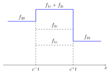
Figure 1: Coordinate dependence of the densities of soliton gases interacting after a collision of soliton clouds with constant initial densities and velocities.

Equations (13) have an obvious degenerate solution, in which $s_{1}$ and $s_{2}$ are constants depending neither on $x$, nor $t$. Despite the triviality of this solution, it has a clear physical meaning: it can serve as a “plateau” connecting two aforementioned solutions in the form of simple waves. In particular, during the collision of mutually penetrating gases with constant densities $f_{1},f_{2}$ and, hence, with Riemann invariants $s_{1},s_{2}$, a region of a two-stream flow is formed, in which the velocities of solitons of one species are renormalized because of their interaction with solitons of the other species. Thus, the problem of collision of two gases is reduced to the determination of densities and velocities of solitons in the region of their “mixing”, as well as the velocities of the edges of this region. Although this problem has already been analyzed in elkamch-05 ; cde-16 , we will briefly consider this problem because the relevant results will be used in further analysis. We assume that at the initial instant, there is a discontinuity in the density distributions for solitons of two species:

$$\left\{\begin{array}[]{lll}f_{2}(x,0)=f_{20},&f_{1}(x,0)=0,&x<0,\\ f_{2}(x,0)=0,&f_{1}(x,0)=f_{10},&x>0,\end{array}\right.$$ (22)

here, we assume that $\kappa_{2}>\kappa_{1}$, so that the faster soliton cloud with density $f_{20}$ overtakes at instant $t=0$ the slower cloud with density $f_{10}$ at point $x=0$ and their mutual penetration begins. As usual, in the case of initial discontinuity the solution must depend only on self-similar variable $\zeta=x/t$. Therefore, the initial discontinuity leads to the formation of a plateau between two simple waves, each of which is a discontinuity with a constant value of one of the Riemann invariants (the existence of such solutions is determined by the aforementioned properties of the Chaplygin gas). In the whole, the solution is a sequence of three flows with constant densities, which are separated by discontinuities:

$$f(x,t)=\left\{\begin{array}[]{ll}f_{20},&x<c^{-}t,\\ f_{1c}+f_{2c},&c^{-}t<x<c^{+}t,\\ f_{10},&x>c^{+}t.\end{array}\right.$$ (23)

It can clearly be seen from Fig. 1 that the leading edge of the plateau moves with renormalized velocity $s_{2c}$ of the fast gas, while the rear edge of the plateau moves with renormalized velocity $s_{1c}$ of the slow gas because the densities at these edges vanish:

$$c^{-}=s_{1c},\qquad c^{+}=s_{2c}.$$ (24)

In the two-flow region $c^{-}t<x<c^{+}t$ of the plateau, the soliton velocities are renormalized by their interaction; in accordance with relations (11) we have

$$\begin{split}&s_{1c}=\frac{\kappa_{1}^{2}(1-\alpha_{2}f_{1c})-\kappa_{2}^{2}\alpha_{1}f_{2c}}{1-\alpha_{1}f_{2c}-\alpha_{2}f_{1c}},\\ &s_{2c}=\frac{\kappa_{2}^{2}(1-\alpha_{1}f_{2c})-\kappa_{1}^{2}\alpha_{2}f_{1c}}{1-\alpha_{1}f_{2c}-\alpha_{2}f_{1c}}.\end{split}$$ (25)

The slow gas flows through the right discontinuity into the plateau region; equating the expressions for its flux on different sides of the discontinuity in the reference frame in which it is at rest, we obtain $f_{1c}(s_{1c}-c^{+})=f_{10}(\kappa_{1}^{2}-c^{+})$. Fast gas flows through the left discontinuity into the plateau region, and analogous calculation gives $f_{20}(\kappa_{2}^{2}-c^{-})=f_{2c}(s_{2c}-c^{-})$. With account for relations (24) and (25) the resulting equalities lead to equations

$$\begin{split}&f_{1c}=f_{10}\frac{s_{2c}-\kappa_{1}^{2}}{s_{2c}-s_{1c}}=f_{10}(1-\alpha_{1}f_{2c}),\\ &f_{2c}=f_{20}\frac{\kappa_{2}^{2}-s_{1c}}{s_{2c}-s_{1c}}=f_{20}(1-\alpha_{2}f_{1c}),\end{split}$$

which gives expressions

$$\begin{split}&f_{1c}=\frac{f_{10}(1-\alpha_{1}f_{20})}{1-\alpha_{1}\alpha_{2}f_{10}f_{20}},\\ &f_{2c}=\frac{f_{20}(1-\alpha_{2}f_{10})}{1-\alpha_{1}\alpha_{2}f_{10}f_{20}},\end{split}$$ (26)

for the densities of the soliton gases in the two-flow region of the plateau. Clearly, these expressions have sense only when the following inequality holds:

$$\alpha_{1}f_{1c}+\alpha_{2}f_{2c}<1,$$ (27)

when renormalized velocities (25) are positive, i.e., the densities of soliton gases cannot be too high. Actually, more stringent limitations on the soliton density are imposed by the condition that variation $\overline{u^{2}}-\overline{u}^{2}$ of the fluctuating wave field in a soliton gas must be positive (see el-16 ). The relations derived above are in good agreement with the results of numerical solution of the KdV equation with the initial data in the form of a large number of solitons of two different species, which are located on different sides of the coordinate origin (see cde-16 ).

V Flow of two soliton gases in the form of a simple wave

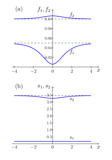
Figure 2: (a) Distributions of densities of soliton gases and (b) of their renormalized velocities as functions of the coordinate for the wave profile defined by formula (34). Soliton gas parameters: $\kappa_{1}=1$, $\kappa_{2}=1.8$, $f_{10}=0.05$, $f_{20}=0.1$. The wave velocity coinciding with the flow velocity of slow solitons is $V=s_{1}=0.174$, while the flow velocity for the fast soliton gas at infinity is $s_{20}=3.469$, which is higher than nonrenormalized velocity $\kappa_{2}^{2}=3.24$.

Expressions (21) give a more general form of the solution for the flow of two soliton gases in the form of a simple wave. Let us suppose that the densities of the soliton gases at infinity tend to constant values:

$$f_{1}\to f_{10},\qquad f_{2}\to f_{20}\qquad\text{as}\qquad x\to\pm\infty.$$ (28)

Then the constant value of Riemann invariant $s_{1}$ is equal to the wave velocity of the soliton gas (see (25))

$$V=s_{1}=\frac{\kappa_{1}^{2}(1-\alpha_{2}f_{10})-\kappa_{2}^{2}\alpha_{1}f_{20}}{1-\alpha_{1}f_{20}-\alpha_{2}f_{10}},$$ (29)

which coincides with the renormalized velocity of the slow gas, while formulas (12) give expressions for the densities of soliton gases:

$$\begin{split}&f_{1}(\xi)=\frac{1}{\alpha_{2}}\left[1+\frac{1}{2}(V-\kappa_{2}^{2})\rho(\xi)\right],\\ &f_{2}(\xi)=\frac{1}{2\alpha_{1}}(\kappa_{1}^{2}-V)\rho(\xi).\end{split}$$ (30)

It can easily be seen that these densities are connected by relation

$$1-\alpha_{1}f_{2}-\alpha_{2}f_{1}=\frac{1}{2}(\kappa_{2}^{2}-\kappa_{1}^{2})\rho,$$ (31)

which implies, in particular, that

$$\rho_{0}=\frac{2(1-\alpha_{1}f_{20}-\alpha_{2}f_{10})}{\kappa_{2}^{2}-\kappa_{1}^{2}}.$$ (32)

Density distributions (30) contain arbitrary function $\rho(\xi)$ and the distribution of the renormalized velocity of the fast soliton gas can also be expressed in terms of this function in accordance with the second expression in (21). At infinity, $s_{2}$ tends to the value (see expressions (25))

$$s_{20}=\frac{\kappa_{2}^{2}(1-\alpha_{1}f_{20})-\kappa_{1}^{2}\alpha_{2}f_{10}}{1-\alpha_{1}f_{20}-\alpha_{2}f_{10}}.$$ (33)

The resulting solution has physical sense for such values of parameters $\kappa_{1},\kappa_{2},f_{10},f_{20}$, that the distribution of densities $f_{1},f_{2}$ of the soliton gases, as well as their renormalized velocities $s_{1},s_{2}$ are positive everywhere.

Figure 2 illustrates the flow for two soliton gases for function $\rho(\xi)$ given by

$$\rho(\xi)=\rho_{0}+\frac{a}{\cosh\xi}.$$ (34)

In this case, the profile of density $f_{1}$ of the slow gas moves together with this component with velocity $V=s_{1}$. The fast gas flows through the slow gas with local velocity $s_{2}$, which decreases in the region of the “well” in distribution $f_{1}$, this leads to an increase in density $f_{2}$ in this region.

VI General solution for the flow of two soliton gases

The hodograph method, which is well known in gas dynamics (see, for example, LL6 ) makes it possible to easily obtain the general solution to Eqs. (13), in the case when both velocities $s_{1}$ and $s_{2}$ vary in space and time. Performing standard hodograph transformation $t=t(s_{1},s_{2})$, $x=x(s_{1},s_{2})$, we reduce these equations to the form

$$\frac{\partial x}{\partial s_{1}}-s_{1}\frac{\partial t}{\partial s_{1}}=0,\qquad\frac{\partial x}{\partial s_{2}}-s_{2}\frac{\partial t}{\partial s_{2}}=0.$$ (35)

Eliminating $x$, we obtain

$$\frac{\partial^{2}t}{\partial s_{1}\partial s_{2}}=\frac{1}{s_{1}}\frac{\partial^{2}x}{\partial s_{1}\partial s_{2}}=\frac{1}{s_{1}}\frac{\partial}{\partial s_{1}}\left({s_{2}}\frac{\partial t}{\partial s_{2}}\right)=\frac{s_{2}}{s_{1}}\frac{\partial^{2}t}{\partial s_{1}\partial s_{2}}.$$

Since $s_{1}\neq s_{2}$, we arrive at equation

$$\frac{\partial^{2}t}{\partial s_{1}\partial s_{2}}=0,$$ (36)

the general solution to which can be written in terms of two arbitrary functions (it is convenient to denote them as $F^{\prime\prime}(s_{1})$ and $G^{\prime\prime}(s_{2})$), in form

$$t(s_{1},s_{2})=F^{\prime\prime}(s_{1})+G^{\prime\prime}(s_{2}).$$ (37)

Equations (35) readily give

$$x(s_{1},s_{2})=s_{1}F^{\prime\prime}(s_{1})+s_{2}G^{\prime\prime}(s_{2})-F^{\prime}(s_{1})-G^{\prime}(s_{2}).$$ (38)

This solution can be transform to

$$\begin{split}&x-s_{1}t=(s_{2}-s_{1})G^{\prime\prime}(s_{2})-F^{\prime}(s_{1})-G^{\prime}(s_{2}),\\ &x-s_{2}t=-(s_{2}-s_{1})F^{\prime\prime}(s_{1})-F^{\prime}(s_{1})-G^{\prime}(s_{2}).\end{split}$$ (39)

In this form, the solution has been obtained in pavlov-87b by a different method.

For completeness of analysis, we consider other representations of the general solution, which may turn out to be more convenient for solving specific problems. If we turn to the hodograph method in the Tsarev form tsarev-90 , the general solution can be written in the form

$$x-s_{2}t=\frac{\partial W}{\partial s_{1}},\qquad x-s_{1}t=\frac{\partial W}{\partial s_{2}},$$ (40)

where function $W=W(s_{1},s_{2})$ must satisfy the Euler-Poisson equation:

$$\frac{\partial^{2}W}{\partial s_{1}\partial s_{2}}+\frac{1}{s_{1}-s_{2}}\left(\frac{\partial W}{\partial s_{1}}-\frac{\partial W}{\partial s_{2}}\right)=0.$$ (41)

It can easily be verified that the solutions to this equation can be expressed in terms of arbitrary functions $F(s_{1})$ and $G(s_{2})$ as follows:

$$W(s_{1},s_{2})=(s_{1}-s_{2})[F^{\prime}(s_{1})-G^{\prime}(s_{2})]-2[F(s_{1})+G(s_{2})].$$ (42)

Substituting this expression into (40), we obtain the solution in form (39). Functions $F(s_{1})$ and $G(s_{2})$ should be determined from the initial conditions to the problem.

As was shown by Riemann (see, for example, sommer-50 ), instead of using this general solution expressed in terms of arbitrary functions, it is often convenient to employ the method in which the solution to the problem is expressed directly in terns of initial conditions with the help of the so-called Riemann function. In our case, the Riemann function can be obtained from the general expression for the polytropic gas dynamics with adiabatic exponent $\gamma=-1$. The hypergeometric function appearing in this expression reduces to $F(-1,2;1;z)=1-2z$ and the Riemann function for Eqs. (13) takes an especially simple form:

$$R(r_{1},r_{2};s_{1},s_{2})=\frac{(r_{1}+r_{2})(s_{1}+s_{2})-2(r_{1}r_{2}-s_{1}s_{2})}{(r_{1}-r_{2})^{2}},$$ (43)

where $(r_{1},r_{2})$ are the current coordinates on the hodograph plane and $(s_{1},s_{2})$ are the coordinates of point $P$, at which the value of function $W=W(P)=W(s_{1},s_{2})$ is sought. We will not write here rather cumbersome general expressions that do not add much for understanding the dynamics of interacting soliton gases; instead of this, we consider the solution to one of typical gas dynamic problems, viz., the problem of expansion of a gas layer. The solution can easily be obtained in elementary form, and its difference from the solutions to the same problem for other physical systems demonstrates well the substantial difference between the conventional gas dynamics and the dynamics of soliton gases.

VII Expansion of a layer from a mixture of two soliton gases

One of typical problems in which a domain of the general solution appears is the problem of expansion of a gas layer. This problem was considered in nk-76 for a classical monatomic gas; in ik-19b for the Bose-Einstein condensate; in ik-20 for a two-temperature plasma, and in landau-53 ; khal-54 ; kamch-19 for an ultrarelativistic gas. In all cases, rarefaction waves propagated from the edges to the bulk of the layer, and after their collision, the general solution domain bordering the rarefaction waves at the edges was formed. However, in the case of a soliton gas, there is no solution in the form of rarefaction waves, and instead of this, discontinuous solutions separated by a plateau with constant values of the Riemann invariants appears. The solution constructed in this way makes it possible to draw certain general conclusions about the evolution of overlapping clouds of soliton gases.

If we assume that a single soliton gas with parameter $\kappa_{1}$ at the initial moment of time has a density distribution in the form of a plateau with value $f_{10}$ for $-l/2\leq x\leq l/2$, its motion at subsequent instants is obvious: this distribution is transferred along the $x$ axis with velocity $\kappa_{1}^{2}$ without change of its shape. If, however, there is a mixture of soliton gases with parameters $\kappa_{1}$ and $\kappa_{2}$, $(\kappa_{1}<\kappa_{2})$ and densities $f_{10}$ and $f_{20}$ at the initial instant in domain $-l/2\leq x\leq l/2$, then the evolution of these gases is more complex: in the course of separation of these gases into two clouds moving with velocities $\kappa_{1}^{2}$ and $\kappa_{2}^{2}$, a two-flow plateau appears. Our aim is the description of the process of spatial separation of soliton clouds and the determination of their parameters after the separation.

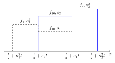
Figure 3: Coordinate dependencies of the densities of two soliton gas clouds during the evolution of the initial layer of two gases before the instant of their separation. Bold dashed line shows the density of the slow gas, while solid line corresponds to the density of the fast gas.

On the plateau formed during the separation, the gases obviously move with renormalized velocities $s_{1},s_{2}$, preserving their initial densities $f_{10},f_{20}$. In front of this layer, there appears a fast gas layer with density $f_{2}$, while behind this layer, a slow gas layer with density $f_{1}$ is formed. The left edge of the overlap region moves with velocity $s_{2}$, while its right edge moves with velocity $s_{1}$. Consequently, the overlap region exists during time

$$T=\frac{l}{s_{2}-s_{1}}$$ (44)

and the gases are separated at $t>T$. It can easily be seen from Fig. 3, that the lengths of the clouds of slow and fast gases at the instant of separation are given by

$$l_{1}=l\cdot\frac{s_{2}-\kappa_{1}^{2}}{s_{2}-s_{1}},\qquad l_{2}=l\cdot\frac{\kappa_{2}^{2}-s_{1}}{s_{2}-s_{1}},$$ (45)

respectively, both of them being smaller than the initial length $l$, because $s_{1}<\kappa_{1}^{2}$ and $s_{2}>\kappa_{2}^{2}$. From the conservation of the number of solitons in each component, we find amplitudes

$$f_{1}=f_{10}\cdot\frac{s_{2}-s_{1}}{s_{2}-\kappa_{1}^{2}},\qquad f_{2}=f_{20}\cdot\frac{s_{2}-s_{1}}{\kappa_{2}^{2}-s_{2}}.$$ (46)

At the instant of separation of the clouds, the centers of mass of the slow soliton cloud and the fast soliton cloud are, respectively, at points

$$x_{1}(T)=\frac{l}{2}\cdot\frac{s_{1}+\kappa_{1}^{2}}{s_{2}-s_{1}},\qquad x_{2}(T)=\frac{l}{2}\cdot\frac{s_{2}+\kappa_{2}^{2}}{s_{2}-s_{1}}.$$ (47)

If solitons did not interact with one another, these clouds would move with nonrenormalized velocities and would be at points $x_{10}(T)=\kappa_{1}^{2}l/(s_{2}-s_{1})$, $x_{20}(T)=\kappa_{2}^{2}l/(s_{2}-s_{1})$ at this instant; i.e., because of the interaction, the clouds are shifted through distances

$$\begin{split}&\Delta x_{1}=x_{1}(T)-x_{10}(T)=\frac{l}{2}\cdot\frac{s_{1}-\kappa_{1}^{2}}{s_{2}-s_{1}}<0,\\ &\Delta x_{2}=x_{2}(T)-x_{20}(T)=\frac{l}{2}\cdot\frac{s_{2}-\kappa_{2}^{2}}{s_{2}-s_{1}}>0.\end{split}$$ (48)

Therefore, because of their interaction, the clouds are narrowed, the soliton densities in both clouds increase, and the slow cloud is shifted backwards, while the fast cloud is shifted in the forward direction. A transition to these values of the shifts are illustrated in Fig. 4, which is obtained from the numerical solution for the Chaplygin gas. At the initial instant, the centers of mass of both gases were at the origin of coordinates, and in the course of separation of the clouds, the center of mass of the fast gas moved more rapidly than it would do with its nonrenormalized velocity, while the center of mass of the slow gas would lag behind the analogous motion with its nonrenormalized velocity. After the instant of separation, the centers of mass of both gases continue their motion with nonrenormalized velocities, acquiring additional shifts due to the interaction with solitons of other species. Good agreement between the values of shifts (48) predicted by the theory and the result of numerical solution means that our idea of the formation of simple waves with discontinuities from the initial discontinuities corresponds to the actual dynamics of interacting soliton clouds in accordance with the kinetic equation.

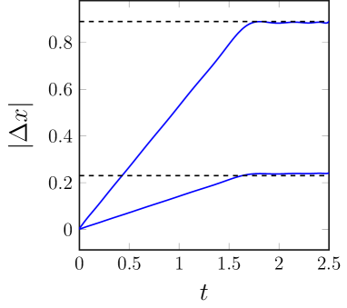
Figure 4: Shifts of the centers of mass of clouds from their positions in the absence of interaction, which are obtained by numerical solution of equations for the Chaplygin gas for the initial values of parameters $f_{10}=0.05$, $f_{20}=0.1$, $\kappa_{1}=1.3$, $\kappa_{2}=2.5$, $l=10$. At instant $T=1.6$ these parameters assume the theoretical values given by formulas (48).

VIII Conclusion

In this study, it is shown that a fundamental property of the dynamics of two interacting soliton gases is the existence of simple waves propagating without a change in form. In particular, such simple waves can have discontinuities; therefore, in problems of the “dam breaking”, instead of rarefaction waves in the dynamic of conventional gases, simple waves appear with discontinuities, which are connected (instead of the general solution in which both Riemann invariants change) by a plateau region with constant Riemann invariants. This property of the dynamics of soliton gases differ drastically from the properties of gas dynamics of conventional gases. At the same time, based on the aforementioned pattern, simple analytic solutions to typical problems, which are confirmed by exact numerical solutions of the kinetic equation reduced to the equivalent form of equations for the dynamics of the Chaplygin gas, can be constructed. The equations constructed in this way lead to an intuitively clear pattern of the behavior of soliton gas clouds: as a result of the interaction, the cloud of fast solitons is shifted in the forward direction, while the cloud of slow solitons is shifted backwards, both clouds becoming narrower and soliton densities increase in both of them. The resulting expressions make it possible to estimate these effects in current experimental investigations of soliton gases in waves on the water surface, in nonlinear optics, and in the physics of cold atoms (see, for example, redor-19 ; suret-20 ; bd-22 ).

The authors are grateful to G. A.  El for fruitful discussions. This study was supported by the Russian Foundation for Basic Research (project no. 20-01-00063).

References

- (1) N. J. Zabusky, M. D. Kruskal, Phys. Rev. Lett. 15, 240 (1965).
- (2) P. D. Lax, Comm. Pure Appl. Math., 21, 467 (1968).
- (3) V. E. Zakharov, S. V. Manakov, S. P. Novikov, and L. P. Pitaevskii, Theory of Solitons: The Inverse Scattering Method, (Nauka, Moscow, 1980; Springer, Berlin, 1984).
- (4) A. C. Newell, Solitons in Mathematics and Physics, (SIAM, Philadelphia, 1985).
- (5) V. E. Zakharov, Sov. Phys. JETP 33, 538 (1971).
- (6) G. A. El, Phys. Lett. A, 311, 374 (2003).
- (7) G. A. El, A. M. Kamchatnov, Phys. Rev. Lett., 95, 204101 (2005).
- (8) G. A. El, A. M. Kamchatnov, M. V. Pavlov, S. A. Zykov, J. Nonlinear Sci., 21, 151 (2011).
- (9) E. V. Ferapontov, M. V. Pavlov, J. Nonlinear Sci., 32, 26 (2022).
- (10) B. Doyon, SciPost Phys. LectNotes, 18, 1 (2020).
- (11) G. A. El, J. Stat. Mech. (2021) 114001.
- (12) I. Redor, E. Barthélemy, H. Michallet, M. Onorato, N. Mordant, Phys. Rev. Lett. 122, 214502 (2019).
- (13) P. Suret, A. Tikan, F. Bonnefoy, F. Copie, G. Ducrozet, A. Gelash, G. Prabhudesai, G. Michel, A. Cazaubiel, E. Falcon, G. El, S. Randoux, Phys. Rev. Lett. 125, 264101 (2020).
- (14) I. Bouchoule, J. Dubail, J. Stat. Mech. 2022, 014003 (2022).
- (15) S. C. Gardner, J. M. Greene, M. D. Kruskal, R. M. Miura, Phys. Rev. Lett., 19, 1095 (1967).
- (16) L. D. Landau and E. M. Lifshitz, Course of Theoretical Physics, Vol. 6: Fluid Mechanics, (Pergamon, New York, 1987; Fizmatlit, Moscow, 2001).
- (17) S. A. Chaplygin, About Gas Jets, (Univ. Tip., Moscow, 1902) [in Russian]; S. A. Chaplygin, Collection of Scientific Works, (OGIZ GITTL, Moscow, 1948), Vol. 2, p. 19 [in Russian].
- (18) F. Carbone, D. Dutykh, G. A. El, EPL, 113, 30003 (2016).
- (19) G. A. El, Chaos, 26, 023105 (2016).
- (20) M. V. Pavlov, Sov. J. Theor. Math. Phys. 73, 1242 (1987).
- (21) S. P. Tsarev, Izv. Akad. Nauk SSSR, Ser. Mat. 54, 1048 (1990).
- (22) A. Sommerfeld, Partial Differential Equations in Physics, Vol. 6 of Lectures on Theoretical Physics (Academic, New York, 1964).
- (23) V. G. Nosov and A. M. Kamchatnov, Sov. Phys. JETP 43, 397 (1976).
- (24) S. K. Ivanov, A. M. Kamchatnov, Phys. Rev. A 99, 013609 (2019).
- (25) S. K. Ivanov, A. M. Kamchatnov, Phys. Fluids, 32, 126115 (2020).
- (26) L. D. Landau, Izv. Akad. Nauk SSSR, Ser. Fiz. 17, 51 (1953).
- (27) I. M. Khalatnikov, Zh. Eksp. Teor. Fiz. 27, 529 (1954).
- (28) A. M. Kamchatnov, J. Exp. Theor. Phys. 129, 607 (2019).