SIR–Model for Households

Abstract

Households play an important role in disease dynamics. Many infections happening there due to the close contact, while mitigation measures mainly target the transmission between households. Therefore, one can see households as boosting the transmission depending on household size. To study the effect of household size and size distribution, we differentiated the within and between household reproduction rate. There are basically no preventive measures, and thus the close contacts can boost the spread. We explicitly incorporated that typically only a fraction of all household members are infected. Thus, viewing the infection of a household of a given size as a splitting process generating a new, small fully infected sub–household and a remaining still susceptible sub–household we derive a compartmental ODE–model for the dynamics of the sub–households. In this setting, the basic reproduction number as well as prevalence and the peak of an infection wave in a population with given households size distribution can be computed analytically. We compare numerical simulation results of this novel household–ODE model with results from an agent–based model using data for realistic household size distributions of different countries. We find good agreement of both models showing the catalytic effect of large households on the overall disease dynamics.

92D30, 93-10

1 Introduction

The spread of an infectious diseases strongly depends on the interaction of the considered individuals. Traditional SIR–type models assume a homogeneous mixing of the population and typically neglect the increased transmission within closed subcommunities like households or school–classes. However, literature indicates, that household transmission plays an important role [4, 3, 9].

In case of the COVID–pandemic, several studies have quantified the secondary attack rate within households, i.e. the probability household-members get infected, given that one household member is infected [10, 12, 7, 3, 9, 11]. The secondary attack rate depends on the virus variant, immunity and vaccination status, cultural differences and mitigation measures within a household (like e.g. early quarantine). In December 2021, when both the Delta and Omicron variants were spreading, it ranged between about 19 % (Delta variant in Norway) [9] to 39 % (Omicron in Spain) [3]. Hence, interestingly, the secondary attack rate within a household is far from 100 % despite the close contacts.

There are several models reported that try to include the contribution of in–household transmission to the overall disease dynamics. The Reed–Frost model describing in–household infections as a Bernoulli–process has be used by [5, 4]. An average model assuming households always get completely infected and ignoring the temporal dynamics has been proposed in [2]. Their findings for the effective reproduction number agree with our results, see (5). Extensions of differential equation based SIR–models in case of a uniform household distribution have be proposed by [6, 8]. However, in real populations, the household distribution is far from uniform, see [14]. Ball and co–authors provided in  [1] an overview of challenges posed by integrating household effects into epidemiological models, in particular in the context of compartmental differential equations models.

In this paper we develop an extended ODE SIR–model for disease transmission within and between households of different sizes. We will treat the infection of a given household as a splitting process generating two new sub–households or household fragments of smaller size - representing the susceptible ($S$) or fully infected ($I$) members. Each of the susceptible household fragments can get infected and split later in time, while infected household segments recover with a certain rate and are then immune (recovered or removed, $R$). The dynamics of the susceptible, infected and recovered household segments is modeled in Section 2. In Section 3, we compute the basic reproduction number for our household model combining the attack rate inside a single households and the transmission rate between individual households. The prevalence, as the limit of the recovered part of the population can be computed analytically — at least in case of small maximal household size, see Section 4. The peak of a single epidemic wave in a population with given household distribution is considered in Section 5. Again, for small maximal household size, we will be able to compute analytically the maximal number of infected. Numerical simulations based on realistic household size distributions for different countries and a comparison with an agent–based model demonstrate the applicability of the presented model. As outlook with focus on non–pharmaceutical interventions we consider an extension of our model quarantining infected sub–households based on a certain detection rate for a single infected.

2 Household Model

Instead of real households we consider effective sub–households or household fragments, still called households throughout this paper, being either fully susceptible, infected or recovered. Let $S_{j},I_{j}$ and $R_{j}$ denote the number of the respective households consisting of $j$ persons, where $1\leq j\leq K$ and $K$ denoting the maximal household size. Then $H_{j}=S_{j}+I_{j}+R_{j}$ equals to the total number of current sub–households of size $j$. Furthermore, we introduce $H=\sum_{j=1}^{K}H_{j}$ as the total number of households and $h_{j}=H_{j}/H$. The total population is given by $N=\sum_{j=1}^{K}jH_{j}$. For further reference we also introduce the first two moments of the household size distribution

$$\mu_{1}:=\sum_{j=1}^{K}jh_{j}\quad\text{and}\quad\mu_{2}:=\sum_{j=1}^{K}j^{2}h_{j}\;.$$

If an infection is brought into a susceptible sub–household of size $j$, secondary infections will occur inside the household. We assume that each of the remaining $j-1$ household members can get infected with probability $a$, called the in–household attack rate. On average, we expect

$$E_{j}=a(j-1)+1$$

infections (including the primary one) inside a household of size $j$. Existing field studies, see [12, 7] indicate an in–household attack rate in the range of $16\%$–$30\%$ depending on the overall epidemiological situation, household size and vaccinations. For the sake of tractability and simplicity, our model assumes a constant attack rate $a$ independent of the household size.

Let $b_{j,k}$ denote the probability, that a primary infection in a household of size $j$ generates in total $k$ infections inside this household, where $1\leq k\leq j$. The secondary infections give rise to a splitting of the initial household of size $j$ into a new, fully infected sub–household of size $k$ and another still susceptible sub–household of size $j-k$.

An infected household of size $k$ recovers with a rate $\gamma_{k}$ and contributes to the overall force of infection by an out–household infection rate $\beta_{k}$. We assume that the out–household reproduction number is independent of the household size, i.e.

(1) $$\mathcal{R}^{\ast}=\frac{\beta_{k}}{\gamma_{k}}=\text{constant independent of $k$}\;.$$

Now, the dynamical system governing the dynamics of the susceptible, infected and recovered households of size $k$ reads as

(2a) $$S_{k}^{\prime} =Y\left[-kS_{k}+\sum_{j=k+1}^{K}\!\!jS_{j}\cdot b_{j,j-k}\right]\;,$$

(2b) $$I_{k}^{\prime} =-\gamma_{k}I_{k}+Y\sum_{j=k}^{K}jS_{j}\cdot b_{j,k}\;,$$

(2c) $$R_{k}^{\prime} =\gamma_{k}I_{k}\;,$$

where

$$Y :=\frac{1}{N}\sum_{k=1}^{K}\beta_{k}\cdot kI_{k}$$

denotes the total force of infection.

For the recovery rate of an infected household of size $k$ we can consider the two extremal cases and an intermediate case.

1. Simultaneous infections: All members of the infected household get infected at the same time and recover at the same time, hence the recovery rate $\gamma_{k}=\gamma_{1}$ is independent of the household size. Assumption (1) leads to a constant out–household infection rate $\beta_{k}=\beta$.

2. Sequential infections: All members of the household get infected one after another and the total recovery time for the entire household equals to $k$ times the individual recovery time. Hence the recovery rate $\gamma_{k}=\gamma_{1}/k$ and by (1) we get $\beta_{k}=\beta_{1}/k$.

3. Parallel infections: The recovery times $T_{i}$, $i=1,\dots,k$ for each of the $k$ infected individuals are modeled as independent exponentially distributed random variables. Hence the entire household is fully recovered at time $\max(T_{1},\dots,T_{k})$. The recovery rate $\gamma_{k}$ equals to the inverse of the expected recovery time, i.e.

   $$\gamma_{k}=\frac{1}{E[\max(T_{1},\dots,T_{k})]}=\frac{1}{E[T_{1}]\cdot\theta_{k}}=\frac{\gamma_{1}}{\theta_{k}}\;,$$

   where $\theta_{k}=1+\tfrac{1}{2}+\dots+\tfrac{1}{k}\sim\log k+g$ denotes the $k$–th harmonic number and $g\approx 0.5772\dots$ denotes the Euler–Mascheroni constant.

All these cases can be subsumed to

$$\gamma_{k}=\frac{\gamma_{1}}{\eta_{k}},\quad\beta_{k}=\frac{\beta_{1}}{\eta_{k}}\;,$$

where $\eta_{k}$ models the details of the temporal dynamics inside an infected household.

In Figure 1 we compare these three cases in the scenario of a population with maximal household size $K=6$. Each household size represents $1/6$ of the entire population. Initially, $1\permil$ of the population is infected. The out–household reproduction number is assumed to be $\mathcal{R}^{\ast}=1.33$, in–household attack rate equals $a=0.2$ and the recovery rate $\gamma_{1}$ for an infected individual equals $0.1$. Shown are the incidences, i.e. the daily new infections over time. The three cases differ in the timing and the height of the peak of the infection; for the simultaneous infections ($\gamma_{k}$ constant) the disease spreads fastest and for the sequential infections ($\gamma_{k}=\gamma_{1}/k$) the spread is significantly delayed. The cases of parallel infections, i.e. $\gamma_{k}\simeq\gamma_{1}/(\log k+g)$, lies between theses two extremes.

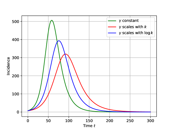
Figure 1: Simulation of one epidemic wave in case of the three different scalings of the recovery rates for households of size $k$. Shown is the incidence, i.e. daily new infections over time. The green curve corresponds equal recovery rates for all households, i.e. $\gamma_{k}=\gamma_{1}$. The red curve corresponds to $\gamma_{k}=\gamma_{1}/k$ (sequential infections). The blue curve corresponds to recovery rates obtaind from the maximum of exponential distributions, i.e. $\gamma_{k}\simeq\gamma_{1}/(\log k)$.

Example 2.1.

Modeling the infections inside the household by a Bernoulli–process with in–household attack rate (infection probability) $a\in[0,1]$, the total number of infected persons inside the household follows a binomial distribution

(3) $$b_{j,k}:=\binom{j-1}{k-1}a^{k-1}(1-a)^{j-k}\;.$$

For the binomial in–household infection (3) it holds, that $E_{j}=a(j-1)+1$.

Theorem 2.2.

In model (2) the total population $N=\sum_{k=1}^{K}k\cdot(S_{k}+I_{k}+R_{k})$ is conserved.

Proof 2.3.

We have

$$N^{\prime}=Y\left[-\sum_{k=1}^{K}k^{2}S_{k}+\sum_{k=1}^{K}k\sum_{j=k+1}^{K}jS_{j}b_{j,j-k}+\sum_{k=1}^{K}k\sum_{j=k}^{K}jS_{j}b_{j,k}\right]$$

We consider the last two summands separately and reverse the order of summation. Hence

$$\sum_{k=1}^{K}k\sum_{j=k}^{K}jS_{j}b_{j,k} =\sum_{j=1}^{K}jS_{j}\sum_{k=1}^{j}kb_{j,k}=\sum_{j=1}^{K}jE_{j}S_{j}$$

and analogously

$$\sum_{k=1}^{K}k\sum_{j=k+1}^{K}jS_{j}b_{j,j-k} =\sum_{j=2}^{K}jS_{j}\sum_{k=1}^{j-1}kb_{j,j-k}$$

$$=\sum_{j=2}^{K}jS_{j}\sum_{l=1}^{j-1}(j-l)b_{j,l}=\sum_{j=2}^{K}jS_{j}\sum_{l=1}^{j}(j-l)b_{j,l}$$

$$=\sum_{j=2}^{K}jS_{j}\left(j\sum_{l=1}^{j}b_{j,l}-\sum_{l=1}^{j}lb_{j,l}\right)=\sum_{j=2}^{K}j^{2}S_{j}-jE_{j}S_{j}$$

$$=\sum_{j=1}^{K}j^{2}S_{j}-jE_{j}S_{j}-\left(S_{1}-E_{1}S_{1}\right)\;.$$

Due to $E_{1}=1$, the last term vanishes. Summing all the contributions, we finally get

$$N^{\prime}=Y\left[\sum_{j=1}^{K}-(j^{2}S_{j})+jE_{j}S_{j}+(j^{2}S_{j}-jE_{j}S_{j})\right]=0\;.$$

3 Basic Reproduction Number

To compute the basic reproduction number for the household–model (2), we follow the next generation matrix approach by Watmough and van den Driessche, see [15]. We split the state variable $x=(S_{1},\dots,R_{K})\in\mathbb{R}^{3K}$ into the infected compartment $\xi=(I_{1},\dots I_{K})\in\mathbb{R}^{K}$ and the remaining components $\chi\in\mathbb{R}^{2K}$. The infected compartment satisfies the differential equation

$$\xi_{k}^{\prime}=\mathcal{F}_{k}(\xi,\chi)-\mathcal{V}_{k}(\xi,\chi)$$

where $\mathcal{F}_{k}=Y\sum_{j=k}^{K}jS_{j}\,b_{j,k}$, $\mathcal{V}_{k}=\gamma_{k}\xi_{k}$ and $Y=\tfrac{1}{N}\sum_{j=1}^{K}\beta_{j}j\xi_{j}$. Now, the Jacobians at the disease free equilibrium $(0,\chi^{\ast})$ are given by

$$F_{kj} =\frac{\operatorname{\partial}\mathcal{F}_{k}}{\operatorname{\partial}\xi_{j}}(0,\chi^{\ast})=\frac{1}{N}j\beta_{j}\sum_{m=k}^{K}mH_{m}\,b_{m,k}$$

$$V_{kk} =\frac{\operatorname{\partial}\mathcal{V}_{k}}{\operatorname{\partial}\xi_{k}}(0,\chi^{\ast})=\gamma_{k}\quad\text{and $V_{kj}=0$ for $k\neq j$}$$

The next generation matrix $G\in\mathbb{R}^{K\times K}$ is given by

$$G =FV^{-1}=\frac{1}{N}\left(\frac{j\beta_{j}}{\gamma_{j}}\sum_{m=k}^{K}mH_{m}\,b_{m,k}\right)_{k,j}$$

Using the relation (1) we obtain

$$G =\mathcal{R}^{\ast}\left(j\sum_{m=k}^{K}\frac{mH_{m}}{N}\,b_{m,k}\right)_{k,j}=\mathcal{R}^{\ast}\begin{pmatrix}\sum_{m=1}^{K}\tfrac{mH_{m}}{N}\,b_{m,1}\\[2.15277pt] \sum_{m=2}^{K}\tfrac{mH_{m}}{N}\,b_{m,2}\\ \vdots\\ \tfrac{KH_{K}}{N}\,b_{KK}\end{pmatrix}\cdot\begin{pmatrix}1,2,\dots,K\end{pmatrix}$$

where the last term represents the next generation matrix as a dyadic product $G=\mathcal{R}^{\ast}\cdot dc^{T}$.

The basic reproduction number $\mathcal{R}=\rho(G)$ is defined as the spectral radius $\rho(G)$ of the next generation matrix $G\in\mathbb{R}^{K\times K}$. As a dyadic product, $G$ has rank one and hence there is only one non–zero eigenvalue.

Lemma 3.1.

Let $c,d\in\mathbb{R}^{n}$ be two vectors with $c^{T}d\neq 0$. The non–zero eigenvalue of the dyadic product $A=dc^{T}\in\mathbb{R}^{n\times n}$ is given by $c^{T}d=\operatorname{tr}(A)$.

Proof 3.2.

Let $v$ be an eigenvector of $A$ to the eigenvalue $\lambda$. Then $\lambda v=Av=(dc^{T})v=(c^{T}v)d$, where $c^{T}v\in\mathbb{R}$. If $\lambda\neq 0$, then $v=\frac{c^{T}v}{\lambda}d$. Set $\mu=\frac{c^{T}v}{\lambda}\in\mathbb{R}$. Now, $Av=A(\mu d)=\mu(dc^{T})d=(c^{T}d)\mu d=(c^{T}d)v$; hence $\lambda=c^{T}d$.

As an immediate consequence we obtain

Theorem 3.3.

The basic reproduction number of system (2) is given by

(4) $$\mathcal{R}=\mathcal{R}^{\ast}\sum_{i=1}^{K}i\sum_{m=i}^{K}\frac{mH_{m}}{N}b_{m,i}=\mathcal{R}^{\ast}\sum_{m=1}^{K}\frac{mH_{m}}{N}E_{m}\;.$$

Corollary 3.4.

In the particular situation, when the expected number of infections inside a household of size $m$ is given by $E_{m}=a(m-1)+1$, the basic reproduction number equals

(5) $$\mathcal{R}=\mathcal{R}^{\ast}\left[1+a\left(\frac{\mu_{2}}{\mu_{1}}-1\right)\right]\;.$$

Assuming, that the infection of any member of a household results in the infection of the entire household, i.e. in–household attack rate $a=1$, our result $\mathcal{R}=\frac{\mu_{2}}{\mu_{1}}\mathcal{R}^{\ast}$ agrees with the result obtained by Becker and Dietz in [2, Sect. 3.2].

4 Computing the prevalence

Let $z=\frac{1}{N}\sum_{k=1}^{K}kR_{k}$ denote the fraction of recovered individuals. Then $z$ satisfies the ODE

$$z^{\prime} =\frac{Y}{\mathcal{R}^{\ast}}\;.$$

In the sequel we will derive an implicit equation for the prevalence $\lim_{t\to\infty}z(t)$ in two special cases:

1. for maximal household size $K=3$. The procedure used here allows for immediate generalization but the resulting expression gets lengthy and provide only minor insight into the result.

2. for in–household attack rate $a=1$ and arbitrary household sizes. In this setting the equations (2a) for the susceptible households decouple and allow and complete computation of the equation for the prevalence.

We will start with the second case. Let us consider $a=1$, i.e. inside households infections are for sure and $E_{k}=k$. Then the ODE for the susceptible households reads as $S_{k}^{\prime}=-YkS_{k}$ and we can insert the recovered $z$

$$S_{k}^{\prime} =-k\mathcal{R}^{\ast}S_{k}z\;.$$

After integration with respect to $$t 0 \infty$$ from to , we get

$$\ln\frac{S_{k}(\infty)}{S_{k}(0)} =k\mathcal{R}^{\ast}\left(z(0)-z(\infty)\right)\;.$$

Assuming initially no recovered individuals, i.e. $z(0)=0$ and considering the total population at the the end of time, i.e. $N=Nz(\infty)+\sum_{k}kS_{k}(\infty)$, we arrive at the system

$$N =Nz(\infty)+\sum_{k=1}^{K}kS_{k}(0)e^{-k\mathcal{R}^{\ast}z(\infty)}\;.$$

Scaling with $$N s_{k,0}=S_{k}(0)/N$$, i.e. introducing , we get

(6) $$1 =z+\sum_{k=1}^{K}k\,s_{k,0}\,e^{-k\mathcal{R}^{\ast}z}\;.$$

In the limit $$\mathcal{R}^{\ast}z\ll 1$$ we obtain the approximation

$$z \sim\frac{1-\sum_{k}ks_{k,0}}{1-\mathcal{R}^{\ast}\sum_{k}k^{2}s_{k,0}}\;.$$

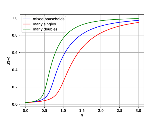
Figure 2: Prevalence in case of maximal household size $K=2$ vs. reproduction number. If double households dominate (green), the prevalence is larger than in the case of mostly single households (red), since households speed up the infection dynamics.

Figure 2 shows the numerical solution of the prevalence equation (6) in case of $K=2$ for reproduction numbers $\mathcal{R}^{\ast}\in[0,3]$ and initially $2\%$ of the entire population being infected. The three different graphs correspond to different initial values for the susceptible households: both single and double households contain $49\%$ of the population (blue), $89\%$ of susceptibles live in single households and only $9\%$ in double households (red) or just $9\%$ in single households and $89\%$ in double households (green).

In case of arbitrary in–household attack rates $a\in[0,1]$, we consider the situation for $K=3$. Setting $z=Z/N$, the relevant equations read as

$$S_{3}^{\prime} =-3\mathcal{R}^{\ast}z^{\prime}\,S_{3}$$

$$S_{2}^{\prime} =\mathcal{R}^{\ast}z^{\prime}\left(-2S_{2}+3b_{3,1}S_{3}\right)$$

$$S_{1}^{\prime} =\mathcal{R}^{\ast}z^{\prime}\left(-S_{1}+2b_{2,1}S_{2}+3b_{3,2}S_{3}\right)\;.$$

Solving the equations successively starting with $S_{3}(t)=S_{3}(0)e^{-3\mathcal{R}^{\ast}z(t)}$ and using variation of constants, we arrive at

$$S_{2}(t) =S_{2}(0)e^{-2\mathcal{R}^{\ast}z(t)}+3b_{3,1}S_{3}(0)\left(1-e^{-\mathcal{R}^{\ast}z(t)}\right)e^{-2\mathcal{R}^{\ast}z(t)}$$

$$S_{1}(t) =S_{1}(0)e^{-\mathcal{R}^{\ast}z(t)}+2b_{2,1}\left(S_{2}(0)+3b_{3,1}S_{3}(0)\right)\left(1-e^{-\mathcal{R}^{\ast}z(t)}\right)e^{-\mathcal{R}^{\ast}z(t)}$$

$$\qquad+\tfrac{3}{2}\left(b_{3,2}-2b_{2,1}b_{3,1}\right)S_{3}(0)\left(1-e^{-2\mathcal{R}^{\ast}z(t)}\right)e^{-\mathcal{R}^{\ast}z(t)}\;.$$

For the prevalence $z=\lim_{t\to\infty}z(t)$ we obtain the implicit equation

(7) $$1=z+\left[s_{1,0}+2b_{2,1}s_{2,0}+3(b_{2,1}b_{3,1}+\tfrac{1}{2}b_{3,2})s_{3,0}\right]e^{-\mathcal{R}^{\ast}z}\\ \qquad+2(1-b_{2,1})\left[s_{2,0}+3b_{3,1}s_{3,0}\right]e^{-2\mathcal{R}^{\ast}z}\\ +3\left[1+(b_{2,1}-2)b_{3,1}-\tfrac{1}{2}b_{3,2}\right]s_{3,0}e^{-3\mathcal{R}^{\ast}z}$$

or in short

$$1=z+c_{1}e^{-\mathcal{R}^{\ast}z}+c_{2}e^{-2\mathcal{R}^{\ast}z}+c_{3}e^{-3\mathcal{R}^{\ast}z}\;,$$

where the coefficients $c_{1},c_{2}$ and $c_{3}$ are the above, rather lengthy expressions involving the initial conditions and the in–household infection probabilities $b_{j,k}$. In case of $K=2$, i.e. setting $s_{3,0}=0$, we get

(8) $$1=z+\left(s_{1,0}+2b_{2,1}s_{2,0}\right)e^{-\mathcal{R}^{\ast}z}+2\left(1-b_{2,1}\right)s_{2,0}e^{-2\mathcal{R}^{\ast}z}\;.$$

In case of arbitrary household size $K>3$, the resulting equation for the prevalence will have the same structure.

For the binomial infection distribution with $a=1$ this reduces to

$$1 =z+s_{1,0}e^{-\mathcal{R}^{\ast}z}+2s_{2,0}e^{-2\mathcal{R}^{\ast}z}+3s_{3,0}e^{-3\mathcal{R}^{\ast}z}$$

and in case of $$a=0$$ we arrive at

$$1 =z+\left(s_{1,0}+2s_{2,0}+3s_{3,0}\right)e^{-\mathcal{R}^{\ast}z}\;.$$

In case of small initial infections, i.e. $s_{1,0}+2s_{2,0}+3s_{3,0}=c_{1}+c_{2}+c_{3}\approx 1$, Eqn. (7) allows for the trivial, disease free solution $z=0$. However, above the threshold $\mathcal{R}_{c}=\frac{1}{c_{1}+2c_{2}+3c_{3}}$ the non–trivial endemic solution shows up. Expanding the exponential for $\mathcal{R}^{\ast}z\ll 1$, we arrive at

$$1\approx z+\left(c_{1}+c_{2}+c_{3}\right)-\mathcal{R}^{\ast}z\left(c_{1}+2c_{2}+3c_{3}\right)+\frac{{\mathcal{R}^{\ast}}^{2}z^{2}}{2}\left(c_{1}+4c_{2}+9c_{3}\right)$$

and hence

$$z\left(\mathcal{R}^{\ast}(c_{1}+2c_{2}+3c_{3})-1\right)\approx\frac{{\mathcal{R}^{\ast}}^{2}z^{2}}{2}\left(c_{1}+4c_{2}+9c_{3}\right)\;.$$

Besides the trivial solution $z=0$, this approximation has the second solution

(9) $$z\simeq\frac{2\left(\mathcal{R}^{\ast}(c_{1}+2c_{2}+3c_{3})-1\right)}{{\mathcal{R}^{\ast}}^{2}\left(c_{1}+4c_{2}+9c_{3}\right)}\;.$$

If $\mathcal{R}^{\ast}>\mathcal{R}_{c}=(c_{1}+2c_{2}+3c_{3})^{-1}$, this second root is positive.

The following Figure 3(left) shows the numerical solution of the prevalence equation (8) in case of $K=2$ for reproduction numbers $\mathcal{R}^{\ast}\in[0,3]$ and initially $2\%$ of the entire population being infected while both single and double households contain $49\%$ of the susceptible population. The different curves show the results depending on the in–household attack rate $a$. The graph on the right depict the case $K=3$ and $s_{1,0}=s_{2,0}=s_{3,0}=\frac{1}{6}$ for three different in–household attack rates $a$. The approximation (9) is shown by the dashed curves. For $\mathcal{R}^{\ast}<\mathcal{R}_{c}$, the trivial disease free solution $z=0$ is the only solution.

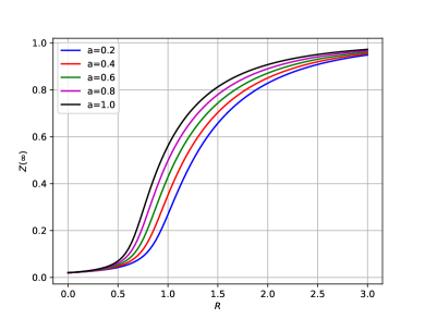
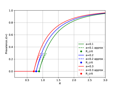
Figure 3: Visualization of the prevalence vs. out–household reproduction number $\mathcal{R}^{\ast}$ and for different in–household attack rate $a$. (Left:) Maximal household size $K=2$. (Right:) Maximal household size $K=3$. Also shown are the asymptotic approximation (9) and the critical value $\mathcal{R}_{c}$.

5 Computing the peak of the infection

Let $J=\sum_{k=1}^{K}kI_{k}$ denote the total number of infected. Then $J$ satisfies

$$J^{\prime} =\sum_{k=1}^{K}kI_{k}^{\prime}=Y\left[-\frac{N}{\mathcal{R}^{\ast}}+\sum_{k=1}^{K}k\sum_{j=k}^{K}jS_{j}b_{j,k}\right]=Y\left[-\frac{N}{\mathcal{R}^{\ast}}+\sum_{j=1}^{K}jS_{j}\sum_{k=1}^{j}kb_{j,k}\right]$$

$$=Y\left[-\frac{N}{\mathcal{R}^{\ast}}+\sum_{j=1}^{K}jS_{j}E_{j}\right]\;.$$

For $K=2$ we have to consider the problem

$$S_{1}^{\prime} =Y\left[-S_{1}+2S_{2}b_{2,1}\right]$$

$$S_{2}^{\prime} =Y\left[-2S_{2}\right]$$

$$J^{\prime} =Y\left[-\frac{N}{\mathcal{R}^{\ast}}+S_{1}+2E_{2}S_{2}\right]\;.$$

Note, that $E_{2}=b_{2,1}+2b_{2,2}$ and $b_{2,1}+b_{2,2}=1$, hence $b_{2,1}=2-E_{2}$. For sake of shorter notation and easier interpretation, we introduce the scaled compartments $s_{1}=S_{1}/N$, $s_{2}=S_{2}/N$ and $j=J/N$. Writing $s_{1}$ as a function of $s_{2}$, we get

$$\frac{ds_{1}}{ds_{2}} =E_{2}-2+\frac{s_{1}}{2s_{2}}$$

with the solution

$$s_{1} =c\sqrt{s_{2}}-2(2-E_{2})s_{2}\;,$$

where $c=2(2-E_{2})\sqrt{s_{2,0}}+s_{1,0}/\sqrt{s_{2,0}}$. For $j$ we have the equation

$$\frac{dj}{ds_{2}} =\frac{-1/\mathcal{R}^{\ast}+s_{1}+2E_{2}s_{2}}{-2s_{2}}=\frac{1}{2\mathcal{R}^{\ast}s_{2}}-\frac{ds_{1}}{ds_{2}}-E_{2}$$

with the solution given by

$$j =\frac{1}{2\mathcal{R}^{\ast}}\ln\frac{s_{2}}{s_{2,0}}-s_{1}(s_{2})-E_{2}(s_{2}-s_{2,0})\;.$$

The maximum of $j$ is either attained in case of an under–critical epidemic at initial time at the necessary condition $j^{\prime}=0$ has to hold. Inserting $s_{1}$ as a function of $s_{2}$ we arrive at the quadratic equation

$$4(E_{2}-1)x^{2}+cx-\frac{1}{\mathcal{R}^{\ast}}=0$$

for $$x=\sqrt{s_{2}}$$ with the positive root

$$x=\sqrt{s_{2}}=\frac{c}{8(E_{2}-1)}\left(\sqrt{1+\frac{16}{\mathcal{R}^{\ast}}\frac{E_{2}-1}{c^{2}}}-1\right)\;.$$

This solution is only meaningful, if $s_{1}+2s_{2}\leq 1$, i.e.

(10) $$\frac{1}{\mathcal{R}^{\ast}}\leq 1+2(E_{2}-1)x^{2}$$

which is an implicit equation for a threshold value of $\mathcal{R}^{\ast}$.

To obtain the value of $j$ at the maximum, we plug this root into the above solution for $j$ and arrive at

$$j_{max} =1-\frac{1}{2\mathcal{R}^{\ast}}\left(1+\ln\frac{s_{2,0}}{x^{2}}\right)-\frac{cx}{2}\;.$$

Hence, the peak of infection $j_{max}$ is a function of the out–household reproduction number $\mathcal{R}^{\ast}=\beta_{k}/\gamma_{k}$, the expected infections in double households $E_{2}$ and the initial conditions $s_{2,0}$, $s_{1,0}$. In particular, it is independent of the scaling of the recovery periods $\gamma_{k}$, as can be seen also in the more complex setting presented in Figure 1.

The following Figure 4 shows the peak of infection $j_{max}$ versus the out–household reproduction number $\mathcal{R}$. Solutions are only plotted, if the condition (10) is satisfied. The left figure shows the situation for $E_{2}=1.5$ and different initial conditions. The right figure shows the variation with respect to $E_{2}=1+a$ keeping the initial conditions fixed as $s_{1,0}=0.5$ and $s_{2,0}=0.25$.

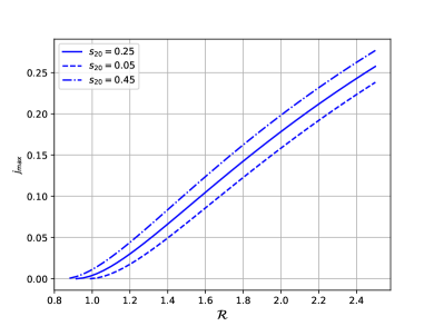
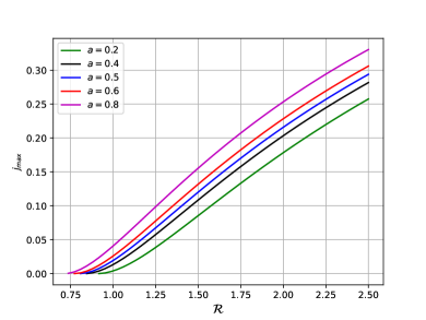
Figure 4: Peak height $j_{\max}$ of a single epidemic wave vs. out–household reproduction number $\mathcal{R}^{\ast}$. (Left:) Variation with respect to different initial household size distributions. (Right:) Variation with respect to different in–household attack rates.

6 Simulations and comparison with agent–based model

The analysis of our household model presented in the previous sections, shows that larger households have a strong effect on the spread of the epidemic. To illustrate this, we simulate a single epidemic wave in populations with close to realistic household distribution. For comparison we choose the household size distributions for Bangladesh (BGD), Germany (GER) and Poland (POL) as published by the UN statistics division in 2011, see [14]. Using a sample of almost $1\,000\,000$ individuals, we obtain the distribution shown in Table 1.

		Number $H_{k}$ of households of size
	Total	$k=1$	$k=2$	$k=3$	$k=4$	$k=5$	$k\geq 6$
Bangladesh	999 995	7 366	24 351	44 022	55 989	42 037	53 960 ($k=7$)
Germany	999 999	173 640	154 920	67 846	48 585	15 201	7 106 ($k=6$)
Poland	999 996	85 032	91 220	71 221	57 605	26 156	22 523 ($k=7$)

Table 1: Distribution of household sizes in Bangladesh, Germany and Poland for the year 2011, see [14]. The sample is based on a scaled population of $1\,000\,000$. Differences are due to round–off effects.

Remark 6.1.

Note, that in Table 1 we have redistributed for Poland and Bangladesh the fraction of population living in households of size $6$ or bigger to household of size equal $7$ to match the total population. How one treats the population represented by the tail in the household distribution can make a substantial difference in the simulation outcomes. To visualize that, we show in Figure 5 simulations for out–household reproduction number $\mathcal{R}^{\ast}=0.9$, in–household attack rate $a=0.2$ and three different versions of how to treat the tail in the Polish household size distribution. The blue curve represents the population distribution given in Table 1. The green curve uses the extended census data including households up to size $10+$. All households of size $10+$ are treated as households of size equal to $10$. The red curve show a simplified treatment of the tail, where all households of size $6+$ are treated as being of size equal to $6$.

The simulation redistributing the households of size $6+$ to size $7$ (blue) agrees within the simulation accuracy with the detailed distribution (green). The simplified treatment (red) shows already a significant difference. This difference will be even more pronounced for smaller reproduction numbers $\mathcal{R}^{\ast}$ since the smaller households first get subcritical with decreasing $\mathcal{R}^{\ast}$. This result clearly visualizes the need for careful treatment of the tail in the household size distribution, since big households have an overproportional impact on the dynamics. Unfortunately, most publicly available data truncates the household size distribution at size $6$. From a modeling and simulation point of view, there is a need for more detailed data on the household size distribution including information for households of size bigger than $6$.

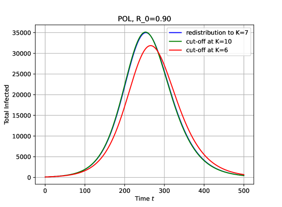
Figure 5: Simulation of one infection wave using different treatment of the tail in the household size distribution. (Blue:) Population distribution given in Table 1 where households of size $6+$ are redistributed to size $7$. (Green:) Polish census data including household sizes up to $10+$. (Red:) Households of size $6+$ treated as being of size equal to $6$.

As initial condition for our simulation we assume $100$ infected single households. The recovery rates inside the households are described using the model of parallel infections, i.e. $\gamma_{k}=\gamma_{1}/(1+1/2+\cdots+1/k)$. For the out–household reproduction number $\mathcal{R}^{\ast}$ we consider the range $0.6\leq\mathcal{R}^{\ast}\leq 2.3$ and the in–household attack is chosen as $a=0.25$. The ODE–system (2) is solved using a standard RK4(5)–method.

Figures 6 and 7 show a comparison of the three countries. The prevalance and the maximum number of infected shown in Fig. 6 clearly visualize that large households are drivers of the infection. For moderate out–household reproduction number $\mathcal{R}^{\ast}\simeq 1$, Bangladesh, with an average household size $\mu_{1}=4.4$, faces a relative prevalence being approx. $50\%$ higher than Germany with an average household size of $\mu_{1}=2.1$ persons. Also the peak number of infected is almost twice as high in Bangladesh compared to Germany for $\mathcal{R}^{\ast}\in[1,1.25]$. Fig. 7 shows the simulation of a single infection wave for moderate out–household reproduction number $\mathcal{R}^{\ast}=1.1$ and in-household attack rate $a=0.25$. The graph illustrates the faster and more severe progression of the epidemics in case of larger households. The peak of the wave occurs in Bangladesh $60$ days earlier and affects almost double the number of individuals compared to Germany.

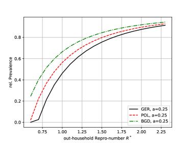
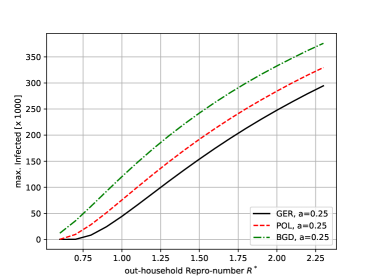
Figure 6: Simulation for countries with different household size distributions according to Table 1. The $x$–axis shows the out–household reproduction number $\mathcal{R}^{\ast}$. The in–household attack rate is fixed as $a=0.25$. Left: Relative Prevalence $z$ after $T=2\,000$ days. Right: Absolute height of peak number of infected $J_{\max}$ (in thousands).

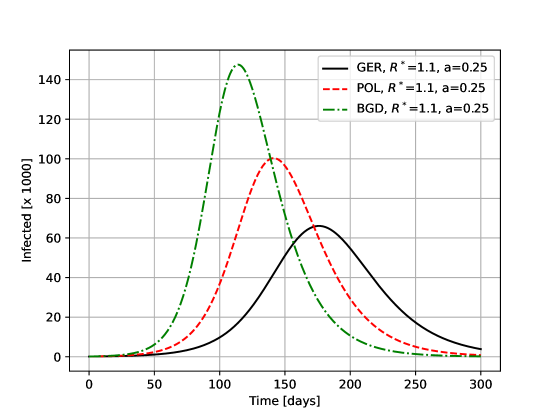
Figure 7: Simulation of one infection wave for countries with different household size distributions according to Table 1. Out–household reproduction number $\mathcal{R}^{\ast}=1.1$ and in–household attack rate $a=0.25$. Plotted is the total number of infected $J$ versus time.

To validate our model, we compared it to a stochastic, microscopic agent–based model developed at the Interdisciplinary Centre for Mathematical and Computational Modelling at the University of Warsaw. Complete details of this model are given in [13]. In this model agents have certain states (susceptible, infected, recovered, hospitalized, deceased, etc.) and infection events occur in certain context, i.e. in households, on the streets or workplaces and several more. Besides the household–context, the street–context is used to capture infection events outside households. Since the ODE–model (2) is a variant of an SIR–model, the agent–based model also just uses the SIR–states and ignores all other states. The agent–based model uses for each infected individual a recovery time that is sampled from an exponential distribution with mean $10$ days. Based on the household distribution for Poland, Figure 8 provides a comparison of the computed prevalence vs. the out–household reproduction number for our model 2 and the agent–based model (blue squares). The solid lines show the results of the ODE–model for different in–household attack rates. The relative prevalence plotted in the figure is defined as the total number of recovered individuals for time $t\to\infty$; here we use $T=2\,000$ days for practical reasons.

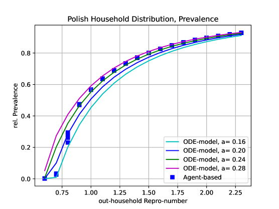
Figure 8: Simulation of one infection wave, plotted is the relative prevalence $z$ versus the out–household reproduction number $\mathcal{R}^{\ast}$. Initially $100$ infected single households in a population according to Table 1. The solid lines show the results of the ODE model for different in–household attack rates. The results of the agent–based model are shown by the blue squares (exponentially distributed recovery time).

Figure 9 shows the results for the peak of the infection wave. The graph on the left shows the peak of the incidences, i.e. the maximum number of daily new infections and the graph on the right shows the time, when this peak occurs.

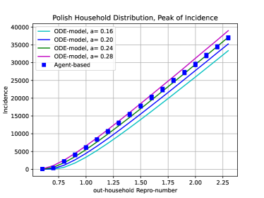
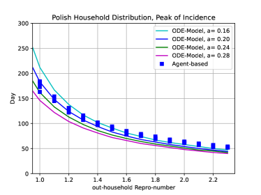
Figure 9: Simulation of one infection wave, initially $100$ infected single households in a population according to Table 1. Left: Peak number of daily new infections versus the out–household reproduction number $\mathcal{R}^{\ast}$. Right: Time, when the peak occurs vs. $\mathcal{R}^{\ast}$. The solid lines show the results of the ODE model for different in–household attack rates. The results of the agent–based model are shown by the blue squares.

For all three presented criteria: prevalence, peak height and peak time, our ODE–household model (2) matches quite well with the agent–based simulation. Best agreement can be seen for in–household attack rate $a$ in the range between $0.16$ and $0.20$.

7 Effect of household quarantine

In this section we will extend our basic model (2) to households put under quarantine after an infection is detected. Therefore, we introduce the additional compartments $Q_{k}$ of quarantined households of size $k$. The extended household model reads as

(11a) $$S_{k}^{\prime} =Y\left[-kS_{k}+\sum_{j=k+1}^{K}\!\!jS_{j}\cdot b_{j,j-k}\right]$$

(11b) $$I_{k}^{\prime} =-\gamma_{k}I_{k}-q_{k}I_{k}+Y\sum_{j=k}^{K}jS_{j}\cdot b_{j,k}$$

(11c) $$Q_{k}^{\prime} =q_{k}I_{k}$$

(11d) $$R_{k}^{\prime} =\gamma_{k}I_{k}$$

Here $q_{k}>0$ denotes the detection and quarantine rate for a household of size $k$.

Let $q>0$ be the probability of infected individual to get detected. The probability that a household consisting of $k$ infected gets detected equals $d_{k}(q)=1-(1-q)^{k}$. Given recovery and detection rates $\gamma_{k}$ and $q_{k}$ for a household of size $k$, the probability, that the household gets detected before recovery equals $q_{k}/(\gamma_{k}+q_{k})$, which equals $d_{k}(q)$. Therefore

$$\frac{q_{k}}{\gamma_{k}}=\frac{d_{k}(q)}{1-d_{k}(q)}\sim kq$$

for $q\ll 1$.

To compute the basic reproduction number, we repeat the computations for the next generation matrix. The vector $\xi$ of infected compartments remains unaltered and the new quarantine compartments $Q_{1},\dots,Q_{K}$ are included in the vector $\chi$. The gain term $\mathcal{F}_{k}$ for the infected compartments remains unaltered as well, but the loss term reads as $\mathcal{V}_{k}=(\gamma_{k}+q_{k})\xi_{k}$. Accordingly, its Jacobian modifies to $V_{kk}=\gamma_{k}+q_{k}$ and finally the next generation matrix $G$ reads as

$$G =\frac{\beta}{N}\left(\frac{j}{\gamma_{j}+q_{j}}\sum_{m=i}^{K}mH_{m}\,b_{m,i}\right)_{i,j}$$

$$=\mathcal{R}^{\ast}\begin{pmatrix}\sum_{m=1}^{K}\tfrac{mH_{m}}{N}\,b_{m,1}\\[2.15277pt] \sum_{m=2}^{K}\tfrac{mH_{m}}{N}\,b_{m,2}\\ \vdots\\ \tfrac{KH_{K}}{N}\,b_{KK}\end{pmatrix}\cdot\begin{pmatrix}\frac{1}{1+q_{k}/\gamma_{k}},\frac{2}{1+q_{2}/\gamma_{2}},\dots,\frac{K}{1+q_{K}/\gamma_{K}}\end{pmatrix}$$

Its non–zero eigenvalue equals

$$\mathcal{R}_{q}:=\mathcal{R}^{\ast}\sum_{k=1}^{K}\frac{k}{1+q_{k}/\gamma_{k}}\sum_{m=k}^{K}\frac{mH_{m}}{N}b_{m,k}=\mathcal{R}^{\ast}\sum_{m=1}^{K}\frac{mH_{m}}{N}\sum_{k=1}^{m}\frac{kb_{m,k}}{1+q_{k}/\gamma_{k}}\;.$$

Due to denominator $1+q_{k}/\gamma_{k}$ we cannot interpret the last sum as the expected infected cases in a household of size $m$. In the asymptotic case of small quarantine rates $q_{k}\ll 1$, we can use the series expansion $(1+q_{k}/\gamma_{k})^{-1}\sim 1-q_{k}/\gamma_{k}\sim 1-kq$ and get

$$\mathcal{R}_{q}\sim\mathcal{R}^{\ast}\sum_{m=1}^{K}\frac{mH_{m}}{N}\left(E_{m}-q\sum_{k=1}^{m}k^{2}b_{m,k}\right)\;.$$

So, the second moment of the in–household infection distribution comes into play.

Remark 7.1.

If the expectation $E_{m}$ and the the second moment $\sum_{k=1}^{m}k^{2}b_{m,k}$ of the in–household infections scale linear with the household size $m$, then the above reproduction number depends on also on the third moment of the household size distribution. This leads to a straight–forward extension of the result (5).

In case of a binomial distribution of the in–household infections, it holds that $E_{m}=a(m-1)+1$ and $\sum_{k=1}^{m}k^{2}b_{m,k}=a(m-1)\left(3+a(m-2)\right)+1$. For the reproduction number we arrive at the expression

$$\mathcal{R}_{q}\sim\mathcal{R}^{\ast}\left[1-\frac{q}{\gamma}+a\left(1-\frac{3q}{\gamma}(1-a)\right)\left(\frac{\mu_{2}}{\mu_{1}}-1\right)-\frac{q}{\gamma}a^{2}\left(\frac{\mu_{3}}{\mu_{1}}-1\right)\right]\;,$$

where $\mu_{3}:=\sum_{k=1}^{K}k^{3}h_{k}$ denotes the third moment of the household size distribution.

The effectiveness of quarantine measures can be assessed by relating the reduction in prevalence to the quarantined individuals. For a given detection probability $q>0$, let $Z(q)$ denote the prevalence observed under these quarantine measures and let $Q(q)$ denote the total number of individuals quarantined. We define the effectiveness of the quarantine measures as

$$\eta_{q}:=\frac{\left|Z(q)-Z(0)\right|}{Q(q)}\;.$$

The numerator equals to the reduction in prevalence and hence $\eta$ can be interpreted as infected cases saved per quarantined case.

In Figure 10 we compare the effectiveness in the setting of household distributions resembling Germany (predominantly small households) and Bangladesh (large households are dominant) for out–household reproduction numbers in the range between $0.9$ and $1.2$. The results indicate, that quarantine measures are less effective in societies with larger households since infection chains inside households are not affected by the quarantine. On the other hand, quarantine measures seem most effective in presence of small households and for low reproduction numbers.

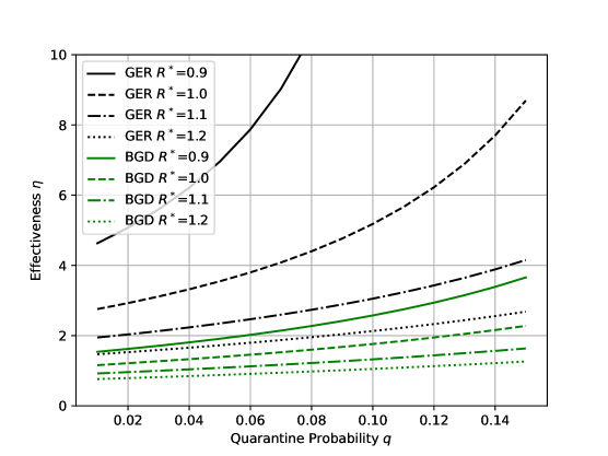
Figure 10: Effectiveness $\eta$ of quarantine measures for the different household distributions in Germany (GER) and Bangladesh (BGD), see Table 1.

8 Conclusion and Outlook

The findings of the compartmental household model (2) are in rather good agreement with microscopic agent–based simulations. Despite its several simplifying assumptions, the prevalence and the peak of the infection wave are reproduced quite well.

However, field data suggests that the in–household attack rate $a$ is significantly higher for $2$–person households than for larger households, see [7, 12]. Analyzing the data given in [7] the attack rate in two–person households is by a factor of $1.25$–$1.5$ larger than in households with three or more members. According to [12] this may be caused by spouse relationship to the index case reflecting intimacy, sleeping in the same room and hence longer or more direct exposure to the index case. An extension of the model (3) to attack rates $a_{k}$ depending on the household size $k$ is straightforward. Carrying over the analytical computation of the reproduction number (5) would lead to a variant of (5) including weighted moments of the household size distribution.

When considering quarantine for entire households, the model shows some interesting outcomes. Defining the ratio of reduction in prevalence and number of quarantined persons as the effectivity of a quarantine, the model suggests that quarantine is more effective in populations where small households dominate. Whether this finding is supported by field data is a topic for future literature research.

Vaccinations are not yet included in the model. From the point of view of public health, the question arises whether the limited resources of vaccines should be distributed with preference to larger households. Given the catalytic effect of large households on the disease dynamics, one could suggest to vaccinate large households first. However, a detailed analysis of this question will be subject of follow–up research.

When extending our ODE SIR–model to an SIRS–model including possible reinfection a recombination of the recovered sub–households is required. Again, this extension will be left for future work. A relaxation of the distribution of the recovered sub–household distribution to the overall household distribution seems a tractable approach to tackle this issue.

References

• [1] F. Ball, T. Britton, T. House, V. Isham, D. Mollison, L. Pellis, and G. S. Tomba, Seven challenges for metapopulation models of epidemics, including households models, Epidemics, 10 (2015), pp. 63–67.
• [2] N. G. Becker and K. Dietz, The effect of household distribution on transmission and control of highly infectious diseases, Mathematical biosciences, 127 (1995), pp. 207–219.
• [3] J. Del Águila-Mejía, R. Wallmann, J. Calvo-Montes, J. Rodríguez-Lozano, T. Valle-Madrazo, and A. Aginagalde-Llorente, Secondary attack rate, transmission and incubation periods, and serial interval of sars-cov-2 omicron variant, spain, Emerging Infectious Diseases, 28 (2022), p. 1224.
• [4] C. Fraser, D. A. Cummings, D. Klinkenberg, D. S. Burke, and N. M. Ferguson, Influenza transmission in households during the 1918 pandemic, American journal of epidemiology, 174 (2011), pp. 505–514.
• [5] K. Glass, J. McCaw, and J. McVernon, Incorporating population dynamics into household models of infectious disease transmission, Epidemics, 3 (2011), pp. 152–158.
• [6] T. House and M. J. Keeling, Deterministic epidemic models with explicit household structure, Mathematical biosciences, 213 (2008), pp. 29–39.
• [7] T. House, H. Riley, L. Pellis, K. B. Pouwels, S. Bacon, A. Eidukas, K. Jahanshahi, R. M. Eggo, and A. Sarah Walker, Inferring risks of coronavirus transmission from community household data, Statistical Methods in Medical Research, 31 (2022), pp. 1738–1756.
• [8] G. Huber, M. Kamb, K. Kawagoe, L. M. Li, B. Veytsman, D. Yllanes, and D. Zigmond, A minimal model for household effects in epidemics, Physical Biology, 17 (2020), p. 065010.
• [9] S. B. Jørgensen, K. Nygård, O. Kacelnik, and K. Telle, Secondary attack rates for omicron and delta variants of sars-cov-2 in norwegian households, JAMA, 327 (2022), pp. 1610–1611.
• [10] W. Li, B. Zhang, J. Lu, S. Liu, Z. Chang, C. Peng, X. Liu, P. Zhang, Y. Ling, K. Tao, et al., Characteristics of household transmission of covid-19, Clinical Infectious Diseases, 71 (2020), pp. 1943–1946.
• [11] F. P. Lyngse, L. H. Mortensen, M. J. Denwood, L. E. Christiansen, C. H. Møller, R. L. Skov, K. Spiess, A. Fomsgaard, R. Lassaunière, M. Rasmussen, et al., Household transmission of the sars-cov-2 omicron variant in denmark, Nature communications, 13 (2022), pp. 1–7.
• [12] Z. J. Madewell, Y. Yang, I. M. Longini, M. E. Halloran, and N. E. Dean, Household transmission of sars-cov-2: a systematic review and meta-analysis, JAMA network open, 3 (2020), pp. e2031756–e2031756.
• [13] K. Niedzielewski, J. M. Nowosielski, R. P. Bartczuk, F. Dreger, Ł. Górski, M. Gruziel-Słomka, A. Kaczorek, J. Kisielewski, B. Krupa, A. Moszyński, et al., The overview, design concepts and details protocol of icm epidemiological model (pdyn 1.5), (2022).
• [14] UN statistics division, Demographic and social statistics. https://unstats.un.org/unsd/demographic-social/products/dyb/documents/household/4.pdf, 2015. Accessed: 2023-01-09.
• [15] P. Van den Driessche and J. Watmough, Reproduction numbers and sub-threshold endemic equilibria for compartmental models of disease transmission, Mathematical biosciences, 180 (2002), pp. 29–48.