On the Influence of Clipping in Lossless Predictive and Wavelet Coding of Noisy Images

Abstract

Especially in lossless image coding the obtainable compression ratio strongly depends on the amount of noise included in the data as all noise has to be coded, too. Different approaches exist for lossless image coding. We analyze the compression performance of three kinds of approaches, namely direct entropy, predictive and wavelet-based coding. The results from our theoretical model are compared to simulated results from standard algorithms that base on the three approaches. As long as no clipping occurs with increasing noise more bits are needed for lossless compression. We will show that for very noisy signals it is more advantageous to directly use an entropy coder without advanced preprocessing steps.

I Introduction

Lossless compression is an important task in all areas where any modification of information is not allowed or at least not acceptable. Examples are among many others measurements for quality assurance, archiving, surveillance, conservation of evidence material or medical data. Noise that is contained in the data has also to be coded in this case. In the medical environment lossy compression is often not acceptable as the correct diagnosis cannot be guaranteed for the lossy coded images. But medical images contain a lot of noise because on the one hand radiation has to be kept low to reduce the risks for the patients and on the other hand the acquisition time is kept short to avoid motion artifacts.

Several different approaches exist for lossless coding. We observed that the performance of the different approaches varies significantly when the data contains different amounts of noise. Prediction-based methods like lossless JPEG [3, 4] and wavelet-based methods like JPEG 2000 [5, 6] are advantageous to code the structural information but become less effective when the images contain a lot of noise. We will provide a theoretical analysis on the behavior of the energy of the noise when a wavelet transform is applied. We will compare this to direct entropy coding and a predictive coding scheme.

Figure 1 shows a block diagram of our signal model. Noise $n\left[k\right]$ with a standard deviation $\sigma$ is added to the signal $s\left[k\right]$ that contains the structural information. The signal $f\left[k\right]$ results from quantizing the noisy signal. One of the methods, i.e., direct, predictive and wavelet, is then applied in the gray box and the output is analyzed. In our study we assume that clipping occurs mainly when the additive noise leads to values that exceed the limits of the quantizer $Q$.

\psfragscanon\psfrag{sigma}{$\sigma$}\psfrag{so}{$f[k]$}\psfrag{si}{}\psfrag{n}{$n[k]$}\psfrag{s}{$s[k]$}\psfrag{Q}{$Q$}\psfrag{H}{$H$}\psfrag{plus}{$+$}\psfrag{noise}{noise}\psfrag{dir}{\emph{direct}}\psfrag{wavelet}{\emph{wavelet}}\psfrag{pr}{\emph{predictive}}\includegraphics[width=216.81pt]{fig/signalmodell}

Figure 1: Signal model

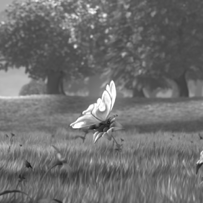
(a) $\uparrow$ / (b) $\downarrow$                          (c)

Figure 2: Two detail images from the Big Buck Bunny sequence (a), (b). (a) is shown with additive noise with $\sigma=30$, (b) is shown original. (c) shows histograms of the image (a) with additive noise (solid red) and original of image (a), i.e., without additive noise (dashed blue)

In Section 2 we present the analysis. The description of our simulation and results are given in Section 3. Section 4 will conclude this study.

II Theoretical Analysis of Noise Impact

We compare three different approaches for coding a signal without loss. The first method is called direct as the samples are directly entropy coded without any preprocessing. The second method is called predictive. Before entropy coding it is possible to subtract a prediction where the predictor for the current sample is computed from already decoded samples. The various predictors differ by the number and the weight of the incorporated samples. We analyze the prediction from one previous sample. The combination of more samples leads to a noise variance reduction due to averaging. But the overall noise variance of the predictor will stay greater than zero. The third class of methods in our analysis is based on the wavelet transform. Instead of subtracting a prediction, the samples are transformed and the coefficients from the sub-bands are then entropy coded. In our analysis we compare two different wavelets, the Haar wavelet and the LeGall 5/3 wavelet.

We assume that the input signal $f\left[k\right]$ consists of the structural information $s\left[k\right]$ with additive noise $n\left[k\right]$ after quantization as shown in Figure 1. For simplicity we show the analysis for the one dimensional case only. At first we neglect the structural part and quantization step. We analyze and compare the output of the different methods. We then show how to calculate the entropy and finally add the structural information of the signal and the quantization step to our modeling.

II-A Noise Variance for Different Coding Methods

For our analysis we are mainly interested in the noise part. We consider the structural signal $s\left[k\right]=0$ in this subsection and assume Gaussian noise $n\left[k\right]$ with zero mean and a variance $\sigma^{2}$. We analyze the influence of the different methods on the noise by comparing the noise variance at their output.

The direct method does not apply preprocessing and so the error distribution does not change and stays equal to

$$\mathcal{E}\left\{n_{\text{direct}}^{2}[k]\right\}=\sigma^{2}.$$ (1)

The second method based on prediction uses one previous sample for the calculation of the predictor $p[k]=f[k-1]$ and will be called predictive. The residuum of the predictor $r[k]=f[k]-p\left[k\right]$ is then coded and the variance of the noise in the resulting sample doubles to

$$\mathcal{E}\left\{n_{p}^{2}[k]\right\}=\mathcal{E}\left\{\left(n[k]-n[k-1]\right)^{2}\right\}=\sigma^{2}+\sigma^{2}=2\sigma^{2}.$$ (2)

Wavelet transforms consist of a filter pair for the computation of the high HP- and the low LP-band. For the Haar wavelet, the samples of the $\text{HP}_{\text{Haar}}$- and the $\text{LP}_{\text{Haar}}$-band are calculated to $\text{HP}_{\text{Haar}}\left[k\right]=f\left[2k\right]-f\left[2k-1\right]$ and $\text{LP}_{\text{Haar}}\left[k\right]=\left\lfloor\frac{1}{2}\left(f\left[2k\right]-f\left[2k-1\right]\right)\right\rfloor$. The rounding operation is due to the integer wavelet transform [1] for lossless coding. The error variance for the coefficients of the $\text{HP}_{\text{Haar}}$ band calculates to

$$\mathcal{E}\left\{n_{\text{HP}_{\text{Haar}}}^{2}[k]\right\}=\mathcal{E}\left\{\left(n[2k]-n[2k-1]\right)^{2}\right\}=2\sigma^{2}.$$ (3)

For the $\text{LP}_{\text{Haar}}$-band the error variance is equal to

$$\mathcal{E}\left\{n_{\text{LP}_{\text{Haar}}}^{2}[k]\right\}=\frac{1}{4}\sigma^{2}+\frac{1}{4}\sigma^{2}=\frac{1}{2}\sigma^{2}.$$ (4)

For the LeGall 5/3 wavelet the samples of the $\text{HP}_{\text{LeGall}}$- and the $\text{LP}_{\text{LeGall}}$- band are calculated to

$$\text{HP}_{\text{LeGall}}\left[k\right]=f\left[2k\right]-\left\lfloor\frac{1}{2}\left(f\left[2k-1\right]+f\left[2k+1\right]\right)\right\rfloor$$ (5)

and

$$\text{LP}_{\text{LeGall}}\left[k\right]=f\left[2k-1\right]+\left\lfloor\frac{1}{4}\left(\text{HP}_{\text{LeGall}}\left[k\right]+\text{HP}_{\text{LeGall}}\left[k-1\right]\right)\right\rfloor$$ (6)

as given in [1]. The error variance for the coefficients of the $\text{HP}_{\text{LeGall}}$-band calculates to

$$\mathcal{E}\left\{n_{\text{HP}_{\text{LeGall}}}^{2}[k]\right\}=\frac{1}{4}\sigma^{2}+\sigma^{2}+\frac{1}{4}\sigma^{2}=\frac{3}{2}\sigma^{2}.$$ (7)

For the $\text{LP}_{\text{LeGall}}$-band the error variance needs to be calculated from the filter representation of the wavelet to preserve the signal independence. The error variance is then equal to

$$\mathcal{E}\left\{n_{\text{LP}_{\text{LeGall}}}^{2}[k]\right\}=\frac{1^{2}+2^{2}+6^{2}+2^{2}+1^{2}}{64}\sigma^{2}=\frac{46}{64}\sigma^{2}.$$ (8)

The combined error variance cannot be computed by averaging the two values $\mathcal{E}\left\{n_{\text{LP}}^{2}\right\}$ and $\mathcal{E}\left\{n_{\text{HP}}^{2}\right\}$ from the subbands. The two subbands are calculated from the same signal values so the independence assumption does not hold anymore. In the next subsection we will show how the values can be combined.

II-B From Noise Variance to Bits

For the wavelet approach a combined variance cannot be computed by simply averaging the variances from the HP- and LP-bands. In order to get an estimation for the number of bits needed for coding the signal processed by the different methods with an optimum entropy coder we use the entropy

$$H=-\sum_{i}p_{i}\text{log}_{2}\left(p_{i}\right)\ \left[\text{bit per sample}\right].$$ (9)

The probabilities $p_{i}$ result from integrals over the probability density function with

$$p_{i}=\int_{i-\frac{1}{2}}^{i+\frac{1}{2}}\frac{1}{\sqrt{2\pi}\sigma^{2}}e^{-\frac{1}{2}\left(\frac{x}{\sigma}\right)^{2}}\,\text{d}x.$$ (10)

Without considering clipping on the upper and lower end of the co-domain $i\in\mathbb{Z}$ holds. For this case (9) can be solved analytically and be approximated by a formula that is dependent on the standard deviation $\sigma$ of the noise

$$H_{\text{direct}}\left(\sigma\right)\approx\log_{2}\left(\sigma\sqrt{2\pi e}\right).$$ (11)

Now we can calculate the entropy for the different methods by evaluating (11) for the variances derived in the previous subsection.

For the predictive scheme the resulting entropy is given by

$$H_{\text{predictive}}\left(\sigma\right)\approx H(\sqrt{2}\sigma)=\frac{1}{2}\,\text{bit}+H_{\text{direct}}\left(\sigma\right).$$ (12)

After the wavelet transform, the signal is represented by coefficients in the high and the low band in a ratio of 1:1. So the overall entropy can be computed by summing up the entropy of the high and the low band containing half the samples each. For the Haar wavelet this results in

$$H_{\text{Haar}}\left(\sigma\right) \approx \frac{1}{2}\left(H\left(\sqrt{\frac{1}{2}}\sigma\right)+H\left(\sqrt{2}\sigma\right)\right)$$

$$= \log_{2}\left(\sigma\sqrt{2\pi e}\right)=H_{\text{direct}}\left(\sigma\right)$$

and for the LeGall 5/3 wavelet in

$$H_{\text{LeGall}}\left(\sigma\right) \approx \frac{1}{2}\left(H\left(\sqrt{\frac{3}{2}}\sigma\right)+H\left(\sqrt{\frac{46}{64}}\sigma\right)\right)$$ (14)

$$= 0.027\,\text{bit}+H_{\text{direct}}\left(\sigma\right).$$

Even though the value range doubles for the $H_{\text{Haar}}$-band that contains half of all coefficients, the entropy of the whole signal stays the same for the Haar wavelet. Comparing the two wavelets, the entropy increases slightly for the LeGall 5/3 wavelet by an offset of $0.027$ bit per sample.

Comparing the entropy of the different methods we can conclude that without clipping all the methods need the same rate for coding the noise up to an offset that does not depend on $\sigma$. While this offset is very small for the wavelet-based methods for the predictive scheme that uses one previous sample the coding of the noise is more expensive by 0.5 bit per sample.

II-C The Influence of Clipping

We now extend the modeling by the structural information and the quantization. As we are interested in lossless coding we are limited to integer values in order to avoid rounding errors. To analyze the impact of clipping to zero mean noise we use a structural signal $s\left[k\right]$ with a constant value in the center of the co-domain $\mu=\left\lceil\frac{2^{8}-1}{2}\right\rceil$. For this we extend (9) by a limitation of $i$. The probabilities $p_{i}$, $i\in 0..255$ for a co-domain of 8 bit, of the signal result from integrating of the probability density function $f_{N}\left(n\right)$ of the noise over the bin size. The calculation of the probabilities $p_{i}$ is given by

$$p_{i}=\begin{cases}\int_{-\infty}^{-127.5}\ f_{N}\left(\nu\right)\,\text{d}\nu&\text{for }i=0\\ \int_{126.5}^{\infty}\ f_{N}\left(\nu\right)\,\text{d}\nu&\text{for }i=255\\ \int_{i-0.5}^{i+0.5}\ f_{N}\left(\nu\right)\,\text{d}\nu&\text{for }0<i<254\end{cases}.$$ (15)

Values outside the co-domain are clipped to the minimum 0 and maximum 255 code value respectively. This leads to peaks in the probability distribution of the signal at the borders of the co-domain as in Figure 2 (c).

In our analysis we assume statistically independent Gaussian noise, so the probability density function of the noise equals $f_{N}\left(n\right)=\frac{1}{\sqrt{2\pi}\sigma^{2}}e^{-\frac{1}{2}\left(\frac{x}{\sigma}\right)^{2}}$. As we assume a signal with a constant code value only, the probability distribution of the signal equals $p_{i}$. The probability distribution of the input signal can now be combined according to the presented methods.

Then the entropy can be calculated by inserting the values of the probabilities from 15 into the entropy formula (9). For the wavelet-based methods the entropy for the HP-band and for the LP-band have to be calculated separately. The resulting values are then summed up by taking into account that each band contains half of the samples.

II-D Theoretical Results

The resulting curves are plotted in Figure 3. The results strongly depend on the $\mu$ chosen for the structural part of the signal. The value of $\mu$ in the center of the co-domain is the ideal case because for a smaller or greater value of $\mu$ clipping is introduced at smaller values of $\sigma$. The plot can be divided into four areas along the abscissa denoted by (a)-(d). In area (a) the noise is quantized to zero and thus has no influence on the entropy. When $\sigma$ gets bigger and only a few samples are affected by noise, that is not quantized to zero, the curves have a different slope as area (b) shows. The reason for the steeper slope of the predictive and wavelet-based methods is the combination of several samples. As soon as the noise component in one sample is above quantization, several coefficients are affected and cause an increase of the entropy. For bigger values of $\sigma$ more samples are affected by noise. As long as the noise is small enough such that no clipping is occurring, the curves run in parallel, as shown in area (c). The offsets correspond to the derivation in the previous subsection. Clipping begins to occur for larger values of the standard deviation $\sigma$ as shown in area (d). Direct entropy coding can exploit the rising number of clipped values better resulting in a lower entropy. The entropy of the predictive scheme and the wavelet-based method drops slower due to the combination of clipped samples with unclipped ones. The LeGall 5/3 wavelet is even more sensitive to this than the Haar wavelet because of the greater filter length.

Figure 3: Theoretical results - entropy in bit per sample plotted over the standard deviation $\sigma$ of the noise on the abscissa in a lin-log plot

III Simulation Results

In our simulation we used different images and added Gaussian noise with increasing standard deviation $\sigma$ before coding them with different algorithms. To validate our model we first used an image of size 512x512 pixels with a constant code value of 128.

(a) (b) (c)

Figure 4: Simulation results show the file size in kbytes over the standard deviation $\sigma$ of the added noise in lin-log plots. (a) shows the results for a constant signal equal to 128. In (b) the results for the first test image (Figure 2 (a)) are shown. (c) shows the results for the second test image (Figure 2 (b))

In order to prove that our model also fits for images we used details from the Big Buck Bunny sequence. The reason for the choice of artificial images is the difficulty of perfectly denoising real images [7]. The chosen images are computer generated and thus do not contain noise in the beginning. We cut images of 512x512 pixels as shown in Figure 2 (a) and (b). For illustration we added Gaussian noise with a standard deviation of $\sigma=30$ to the first detail shown in Figure 2 (a). The second detail in Figure 2 (b) is shown in original, i.e., without additive noise. In our simulation we used the green color channel only.

For direct entropy coding we used bzip2 [2] in version 1.0.4. No additional parameters were given when calling the program. For predictive coding we used lossless JPEG [3, 4]. For wavelet-based coding we used JPEG 2000 [5, 6] with 4 decomposition steps. As long as the number of decomposition steps is larger than 3 this parameter has not much influence on the file size.

The results are shown in Figure 4 where the file size of the compressed images is plotted in kbyte over the standard deviation $\sigma$ of the noise in lin-log plots.

In Figure 4 (a) the results are shown for the image with a constant code value of 128 and additive noise. By comparing Figure 4 (a) with the theoretical results in Figure 3 it can be seen that our model matches with the results from the simulation up to the offset of the lossless JPEG method for small values of $\sigma$. The corresponding curves have the same shape and the plot in Figure 4 (a) can also be divided into the four areas indicated in Figure 3.

Quantitative statements cannot be given as the results strongly depend on the structural information in the input signal.

The offsets in Figure 4 (b) and (c) come from the structural information. The three methods need a different amount of bits to code the structural information. The two plots show clearly that as long as the noise part is small enough advanced methods as a predictive scheme and a wavelet decomposition are advantageous because they are more capable to reduce the redundancy in the structural information part of the signal.

Clipping in the structural information, e.g. due to wrong exposure, often affects bigger areas of an image and thus is beneficial for predictive and wavelet-based coding. The problem are isolated clipped values introduced by noise because their combination with other unclipped samples lead to a higher entropy.

The results in Figure 3 and Figure 4 (a) show that it is advantageous to use direct entropy coding for noise. In [7] several state of the art denoising algorithms are compared to a theoretical bound. The result is that there is still room for improvements. A separation of the noise from the structural information leads to an increase of the encoder complexity. The decoder has to decode both parts and add the noise to the structural part. Compared with wavelet-based coding gains can be achieved for small values of $\sigma$ as shown in area (b) of Figure 3.

Another result is that for very noisy images when clipping is introduced by noise it is more advantageous to directly use an entropy coder without any signal decomposition. These results show that our model also fits for images with structural information.

IV Conclusion

In this paper we analyzed the impact of clipping to lossless compression of noisy images. We derived an analytical description that models the behavior of different coding methods. So the effects shown are general properties of the methods and not of a special implementation. Simulation results support our model. The results show that in general for noisy data it is advantageous to code the noise and the signal separately. Furthermore, the results show that for the case that clipping is introduced by noise it is more advantageous to directly use an entropy coder without advanced preprocessing steps.

References

- [1] A. Calderbank, I. Daubechies, W. Sweldens, and B.-L. Yeo, “Lossless image compression using integer to integer wavelet transforms,” in Int. Conf. on Image Processing (ICIP), vol. 1, pp. 596–599, oct. 1997.
- [2] J. Seward, “bzip2 and libbzip2: A program and library for data compression,” http://www.bzip.org.
- [3] ISO/IEC JTC1/SC29/ WG1 and ITU-T (JPEG), “ISO/IEC IS 10918-1:1994 | ITU-T Rec. T.81 Information technology - Digital compression and coding of continuous-tone still images: Requirements and guidelines,” 1994.
- [4] G. Wallace, “The JPEG still picture compression standard,” IEEE Trans. on Consumer Electronics, vol. 38, no. 1, pp. 18–34, feb. 1992.
- [5] ISO/IEC JTC1/SC29/ WG1 and ITU-T SG-8 (JPEG), “ISO/IEC 15444-1:2004 | ITU-T Rec. T.800 JPEG 2000 Image Coding System, Part 1: Core Coding System,” 2000.
- [6] C. Christopoulos, A. Skodras, and T. Ebrahimi, “The JPEG2000 still image coding system: an overview,” IEEE Trans. on Consumer Electronics, vol. 46, no. 4, pp. 1103–1127, nov. 2002.
- [7] P. Chatterjee and P. Milanfar, “Fundamental limits of image denoising: Are we there yet?” in IEEE Int. Conf. on Acoustics Speech and Signal Processing (ICASSP), pp. 1358–1361, mar. 2010.