Dissipation Dynamics Driven Transitions of the Density Matrix Topology

Abstract

The dynamical evolution of an open quantum system can be governed by the Lindblad equation of the density matrix. In this letter, we propose that the density matrix topology can undergo a transition during the Lindbladian dynamical evolution. Here we characterize the density matrix topology by the topological invariant of its modular Hamiltonian. We focus on the fermionic Gaussian state, where the modular Hamiltonian is a quadratic operator of a set of fermionic operators. The topological classification of such Hamiltonians depends on their symmetry classes. Hence, a primary issue we deal with in this work is to determine the requirement for the Lindbladian operators, under which the modular Hamiltonian can maintain its symmetry class during the dynamical evolution. When these conditions are satisfied, along with a nontrivial topological classification of the symmetry class of the modular Hamiltonian, a topological transition can occur as time evolves. We present two examples of dissipation driven topological transitions where the modular Hamiltonian lies in the AIII class with $U(1)$ symmetry and in the DIII class without $U(1)$ symmetry, respectively. As a manifestation of the topological transition, we present the signature of the eigenvalues of the density matrix at the transition point.

In the past decades, topology has been extensively used to characterize the ground state wavefunction of a quantum Hamiltonian. In such situations, the topology of the wavefunction and the topology of the Hamiltonian are directly related. One of the most well-established situations is the insulators of free fermions Hasan10 ; TIreview ; TIbook . Another important lesson we have learned is the close relationship between the symmetry of a Hamiltonian and its topological classification Schnyder08 ; Kitaev09 ; Symmetry_RMP . In many cases, topologically nontrivial states exist only when certain symmetries are enforced. For free fermion insulators and superconductors, this leads to the celebrated Altland-Zirnbauer ten-fold way classification tenfold of topological states using time-reversal, particle-hole, and chiral symmetries Schnyder08 ; Kitaev09 ; Symmetry_RMP .

In recent years, there has been an increasing interest in studying topological properties for non-equilibrium dynamics. In some non-equilibrium situations, the quantum state remains a pure state, but is no longer an eigenstate of the system. A typical situation is quench dynamics Quench-1 ; Quench-2 ; Quench-3 ; Quench-4 ; Quench-5 ; Quench-6 ; Quench-7 ; Quench-8 , where an initial pure state undergoes unitary dynamical evolution governed by the system’s Hamiltonian. It has been shown that a properly defined topology of the wavefunction dynamics can still reveal the topology of the system’s Hamiltonian Quench-1 ; Quench-2 ; Quench-3 ; Quench-4 ; Quench-5 ; Quench-6 ; Quench-7 ; Quench-8 . Nevertheless, in more generic non-equilibrium situations, the quantum state is not even a pure state but a mixed state described by a density matrix. These situations include finite temperature and open systems with dissipation.

An open quantum system is described by a density matrix $\hat{\rho}$ whose evolution is governed by the Lindblad equation lindblad1 ; lindblad2 . Since the Lindbladian evolution can be viewed as evolution under non-hermitian Hamiltonian in doubled Hilbert space, there are works on open system topology by considering the topology of Lindbladian itself top_lind1 ; top_lind2 ; top_lind3 . At sufficiently long time, an open system can reach a non-equilibrium steady state that does not evolve. There are also extensive works focusing on the topological properties of the non-equilibrium steady states top_dis1 ; top_dis2 ; top_dis3 ; top_dis4 ; top_dis5 ; top_dis6 ; top_dis7 ; top_dis8 ; top_dis9 .

On the other hand, the topology of density matrix itself attracts attention top_dens1 ; top_dens2 ; top_dens3 ; top_dens4 ; top_dens5 ; top_dens6 ; top_dens7 ; top_dens8 . The basic idea is to consider the modular Hamiltonian $\hat{K}$ by writing $\hat{\rho}=e^{-\hat{K}}$. The modular Hamiltonian is always a Hermitian operator, and the topology of the modular Hamiltonian can characterize the topology of the density matrix top_dens3 ; top_dens5 ; top_dens8 . The modular Hamiltonian changes in time when the density matrix evolves under the Lindbladian dynamics. In this letter, we address the issue of whether the modular Hamiltonian can undergo a topological transition as time evolves in the Lindbladian dynamics of an open system. This question concerns the entire dissipation-driven dynamical process instead of the long-time steady state. The answer to this question should depend on both the Lindbladian operator and the choice of the initial state. This distinguishes our work from the previous studies of open-system topology top_lind1 ; top_lind2 ; top_lind3 ; top_dis1 ; top_dis2 ; top_dis3 ; top_dis4 ; top_dis5 ; top_dis6 ; top_dis7 ; top_dis8 ; top_dis9 .

Here we consider the Gaussian state of a set of fermion operators. A gaussian state can be viewed as a non-equilibrium generalization of free-fermion state, whose modular Hamiltonian is a quadratic operator of a set of fermion operators gauss1 ; gauss2 . Hence, we can utilize the existing knowledge of classifying such quadratic fermionic Hamiltonian. It is known that the topological classification of such quadratic Hamiltonians requires understanding its symmetry class Symmetry_RMP ; Schnyder08 ; Kitaev09 . In this work, we consider a generic non-equilibrium situation where the modular Hamiltonian of the initial state have no relation with the system’s Hamiltonian and can lie in a different symmetry class. Hence, primarily to address the dissipation-driven topological transition, we first need to consider another issue: under what conditions the Lindbladian evolution can preserve the symmetry of a modular Hamiltonian?

Symmetry Preserving Lindbladian. The time evolution of the density matrix of an open system is governed by the Lindblad equationlindblad1 ; lindblad2

$$\frac{d\hat{\rho}}{dt}=-i[\hat{H},\hat{\rho}]+\sum\limits_{\mu}(2\hat{L}_{\mu}\hat{\rho}\hat{L}^{\dagger}_{\mu}-\{\hat{L}^{\dagger}_{\mu}\hat{L}_{\mu},\hat{\rho}\}).$$ (1)

We consider Gaussian initial state $\hat{\rho}(t=0)$ of a set of fermion operators $\{\hat{c}^{\dagger}_{i}\}$. The Hamiltonian $\hat{H}$ is a quadratic operator of these fermion operators, and all $\hat{L}_{\mu}$ are linear in these fermion operators, under which a Gaussian state can remain a Gaussian one during the Lindblad time evolution gauss2 ; correlation1 ; correlation2 . In this work, we deal with the most generic situations that $\hat{K}$, $\hat{H}$ and $\hat{L}_{\mu}$ do not commute with each other.

We first study the cases that both the modular Hamiltonian and the Lindbladian possess a global $U(1)$ symmetry. This $U(1)$ symmetry can be either a spin $U(1)$ or a charge $U(1)$ symmetry. When interpreted as a charge (spin) $U(1)$ symmetry, the corresponding class describes insulators (superconductors). For superconductors with the spin $U(1)$ symmetry, one can always apply a particle-hole transformation to map the spin $U(1)$ symmetry into a charge $U(1)$ symmetry. Therefore, we present the following discussions in the context of the charge $U(1)$ symmetry.

With the presence of the charge $U(1)$ symmetry, we can write $\hat{K}=\sum_{ij}K_{ij}\hat{c}^{\dagger}_{i}\hat{c}_{j}$, and $\hat{H}=\sum_{ij}h_{ij}\hat{c}^{\dagger}_{i}\hat{c}_{j}$. Each dissipation operator should be either pure loss term as a superposition of annihilation operators, denoted by $\hat{L}^{l}_{\mu}=\sum_{\mu,i}D^{l}_{\mu i}\hat{c}_{i}$, or pure gain term as a superposition of creation operators $\hat{L}^{g}_{\mu}=\sum_{\mu,i}D^{g}_{\mu i}\hat{c}^{\dagger}_{i}$. In other words, each single dissipation operator cannot contain both creation and annihilation operators. $K_{ij}$, $h_{ij}$, $D^{l}_{\mu i}$ and $D^{g}_{\mu i}$ are matrices or vectors written in the single particle bases.

Below we should study how the modular Hamiltonian matrix $K$ evolves in time. Nevertheless, the matrix $K$ obeys a non-linear equation which complicates the analyzing process. On the other hand, another important property of a Gaussian state is that the two-point correlation contains all the information of this state, and all the higher-order correlations can be expressed in terms of two-point corrections. Thus, instead of considering the dynamics of the matrix $K_{ij}$, we can consider the correlation matrix $C$, defined as $C_{ij}=\mathrm{Tr}(\hat{c}^{\dagger}_{i}\hat{c}_{j}\hat{\rho})$. It is important to note that the correlation matrix $C$ obeys a linear equation. For cases with the $U(1)$ symmetry, the correlation matrix and the modular Hamiltonian matrix are related by correlation1 ; correlation2

$$C=\frac{1}{e^{K^{\text{T}}}+1},$$ (2)

where “T” stands for transpose. Following the Lindblad equation, it can be shown that the correlation matrix obeys the following linear equation correlation1 ; correlation2 ; correlation3

$$\frac{dC}{dt}=XC+CX^{\dagger}+2M^{g}$$ (3)

where the matrix $X$ is defined as $X=iH^{\text{T}}-(M^{l})^{\text{T}}-M^{g}$ and $H$ is the physical Hamiltonian matrix. Here the matrix $M^{l}$ is from the loss terms, defined as $M^{l}_{ij}=\sum_{\mu}D^{l*}_{\mu i}D^{l}_{\mu j}$, and the matrix $M^{g}$ is from the gain terms $M^{g}_{ij}=\sum_{\mu}D^{g*}_{\mu i}D^{g}_{\mu j}$.

Following the ten-fold way classification, we consider the time-reversal symmetry $\mathcal{T}$, the particle-hole symmetry $\mathcal{C}$ and the chiral symmetry $\mathcal{S}$ of the modular Hamiltonian matrix $K$. Here we should clarify that the time-reversal symmetry should not be understood as a physical time reversal of the system. Instead, it merely means an antiunitary transformation that changes $K$ by $U^{\dagger}_{\mathcal{T}}KU_{\mathcal{T}}=K^{*}$, where $U_{\mathcal{T}}$ is the unitary part of $\mathcal{T}$ symmetry.

First we derive the conditions to preserve $\mathcal{T}$ symmetry. Using Eq. 2, $\mathcal{T}$ symmetry leads to $C^{\text{T}}U_{\mathcal{T}}=U_{\mathcal{T}}C$. That is to say, initially, $C^{\text{T}}U_{\mathcal{T}}-U_{\mathcal{T}}C=0$. If the Lindblad evolution can keep the $\mathcal{T}$ symmetry of the modular Hamiltonian, it requires $d(C^{\text{T}}U_{\mathcal{T}}-U_{\mathcal{T}}C)/dt=0$. It is easy to show that

$$\frac{d}{dt}(C^{\text{T}}U_{\mathcal{T}}-U_{\mathcal{T}}C)=(X^{*}U_{\mathcal{T}}-U_{\mathcal{T}}X)C$$

$$+C^{\text{T}}(X^{\text{T}}U_{\mathcal{T}}-U_{\mathcal{T}}X^{\dagger})+2(M^{g}U_{\mathcal{T}}-U_{\mathcal{T}}M^{g}).$$ (4)

Since we consider generic initial states with $\mathcal{T}$ symmetry, the requirement $d(C^{\text{T}}U_{\mathcal{T}}-U_{\mathcal{T}}C^{\text{T}})/dt=0$ leads to $X^{*}U_{\mathcal{T}}-U_{\mathcal{T}}X=0$, $X^{\text{T}}U_{\mathcal{T}}-U_{\mathcal{T}}X^{\dagger}=0$ and $M^{g}U_{\mathcal{T}}-U_{\mathcal{T}}M^{g}=0$. These conditions can be further simplified as

$$U^{\dagger}_{\mathcal{T}}HU_{\mathcal{T}}=-H^{*},U^{\dagger}_{\mathcal{T}}M^{l}U_{\mathcal{T}}=(M^{l})^{*},U^{\dagger}_{\mathcal{T}}(M^{g})^{*}U_{\mathcal{T}}=M^{g}.$$ (5)

In other words, if the modular Hamiltonian of the initial state has $\mathcal{T}$ symmetry, and the Hamiltonian and the dissipation operators satisfy Eq. 5, the $\mathcal{T}$ symmetry will be preserved during the entire Lindbladian dynamics. Especially, we note that the required symmetry property for the physical Hamiltonian $H$ is different compared with the symmetry property of the modular Hamiltonian $K$.

Next, we consider the particle-hole symmetry $\mathcal{C}$. With this symmetry the modular Hamiltonian matrix transfers as $U^{\dagger}_{\mathcal{C}}KU_{\mathcal{C}}=-K^{*}$ under a unitary matrix $U_{\mathcal{C}}$. This is equivalent to $C^{\text{T}}U_{\mathcal{C}}+U_{\mathcal{C}}C-U_{\mathcal{C}}=0$. Hence, in order to preserve the particle-hole symmetry, we require $d(C^{\text{T}}U_{\mathcal{C}}+U_{\mathcal{C}}C-U_{\mathcal{C}})/dt=0$. Similar analysis as above leads to following conditions

$$U^{\dagger}_{\mathcal{C}}HU_{\mathcal{C}}=-H^{*},U^{\dagger}_{\mathcal{C}}M^{l}U_{\mathcal{C}}=M^{g},U^{\dagger}_{\mathcal{C}}(M^{g})^{*}U_{\mathcal{C}}=(M^{l})^{*}.$$ (6)

We note that preserving the particle-hole symmetry requires simultaneously presence both the loss and the gain terms.

Finally we consider the chiral symmetry $\mathcal{S}$ under which the modular Hamiltonian matrix transfers as $U^{\dagger}_{\mathcal{S}}KU_{\mathcal{S}}=-K$, equivalent to $C^{\text{T}}U_{\mathcal{S}}+U_{\mathcal{S}}C^{\text{T}}-U=0$. Hence, to preserve the chiral symmetry, we require $d(C^{\text{T}}U_{\mathcal{S}}+U_{\mathcal{S}}C^{\text{T}}-U_{\mathcal{S}})/dt=0$. Following the same spirit, we arrive at

$$U^{\dagger}_{\mathcal{S}}HU_{\mathcal{S}}=H,U^{\dagger}_{\mathcal{S}}M^{l}U_{\mathcal{S}}=(M^{g})^{*},U^{\dagger}_{\mathcal{S}}(M^{g})^{*}U_{\mathcal{S}}=M^{l}.$$ (7)

Time-reversal and the particle-hole symmetries automatically guarantees the chiral symmetry by taking $U_{\mathcal{S}}=U_{\mathcal{C}}U_{\mathcal{T}}^{*}$. As a self-consistent check, it is easy to prove that Eq. 5 and Eq. 6 automatically ensure Eq. 7.

Eq. 5, Eq. 6 and Eq. 7 respectively give the conditions for preserving $\mathcal{T}$, $\mathcal{C}$ and $\mathcal{S}$ symmetries of the modular Hamiltonian when the system and initial states are $U(1)$ symmetric. Next, we move to the situation without charge or spin $U(1)$ symmetry, such as the cases with fermion pairing between same spins. In this case, we use the Nambu spinor by introducing $\hat{\Psi}=(\hat{c}_{1},\dots,\hat{c}_{N},\hat{c}^{\dagger}_{1},\dots,\hat{c}^{\dagger}_{N})^{\text{T}}$, and we write the physical and the modular Hamiltonians into the Bogoliubov form as $\hat{H}=\hat{\Psi}^{\dagger}H\hat{\Psi}$ and $\hat{K}=\hat{\Psi}^{\dagger}K\hat{\Psi}$. Unlike the cases with $U(1)$ symmetry, the dissipation operators can be a superposition of both loss and gain as $\hat{L}_{\mu}=D^{l}_{\mu i}\hat{c}_{i}+D^{g}_{\mu i}\hat{c}^{\dagger}_{i}$. We introduce the correlation matrix as $C$ as $C_{ij}=\mathrm{Tr}(\hat{\Psi}^{\dagger}_{i}\hat{\Psi}_{j}\hat{\rho})$ that includes anomalous correlations. Now the correlation matrix and the modular Hamiltonian matrix are related by

$$C=\frac{1}{e^{2K^{\text{T}}}+1}.$$ (8)

Similarly, we can define the matrix $M^{l}$ and $M^{g}$ as introduced above and two extra matrices $M^{lg}_{ij}=\sum_{\mu}D^{l*}_{\mu i}D^{g}_{\mu j}$ and $M^{gl}_{ij}=\sum_{\mu}D^{g*}_{\mu i}D^{l}_{\mu j}$. Following the Lindblad equation, the correlation matrix $C$ now obeys the linear equation

$$\frac{dC}{dt}=XC+CX^{\dagger}+2W.$$ (9)

Here the matrix $X=2iH^{\text{T}}-M^{\text{T}}-W$, and the matrices $M$ and $W$ are respectively written

$$M=\left(\begin{array}[]{cc}M^{l}&M^{lg}\\ M^{gl}&M^{g}\end{array}\right),\ \ W=\left(\begin{array}[]{cc}M^{g}&M^{gl}\\ M^{lg}&M^{l}\end{array}\right).$$ (10)

Since the Bogoliubov Hamiltonian automatically possesses the particle-hole symmetry, we only need to investigate the time-reversal symmetry. The derivation of the symmetry preserving condition is very similar to the case with $U(1)$ symmetry above. The results are

$$U^{\dagger}_{\mathcal{T}}HU_{\mathcal{T}}=-H^{*},U^{\dagger}_{\mathcal{T}}MU_{\mathcal{T}}=M^{*},U^{\dagger}_{\mathcal{T}}W^{*}U_{\mathcal{T}}=W.$$ (11)

Hence we have succeeded in deriving the conditions for Lindbladian to preserve $\mathcal{T}$, $\mathcal{C}$ and $\mathcal{S}$ symmetries with and without $U(1)$ symmetry.

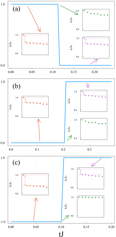
Figure 1: Topological transition of the density matrix during the Lindbladian evolution. The vertical axis is the topological invariant of the modular Hamiltonian and the horizontal axis is time $t$ in unit of hopping $J$. (a-b) Example I. The modular Hamiltonian is a one-dimension SSH model in the AIII class. $J=(J_{1}+J_{2})/2$. (a) $J_{1}=0.8J$ and $J_{2}=1.2J$, $\gamma_{1}=0.8J$ and $\gamma_{2}=0.4J$; (b) $J_{1}=1.2J$ and $J_{2}=0.8J$, $\gamma_{1}=0.4J$ and $\gamma_{2}=0.8J$. $\delta=0.1J$ for both (a) and (b). (c) Example II. The modular Hamiltonian belongs to two-dimensional square lattice pairing model in DIII class. We set $\mu=1.0J$, $\Delta_{0}=1.0J$, $w=0.5J$, $\gamma_{1}=0.4J$ and $\gamma_{2}=0.6J$. The insets show the ratio $\lambda_{i}/\lambda_{0}$ between a few of the largest eigenvalues of the density matrix, with $\lambda_{0}$ the largest eigenvalue.

Examples of Topological Transition. Now we give concrete examples of topological transition. It is easy to see that when the following three conditions are satisfied, the modular Hamiltonian must undergo a topological transition during the dissipation dynamics. First, the initial modular Hamiltonian must lie in a symmetry class and dimension which hosts nontrivial topological classification. Secondly, the Lindbladian must satisfy the abovementioned conditions to preserve this symmetry class. Thirdly, the modular Hamiltonians of the initial state and the long-time steady state are both gapped and have different topological numbers. Below we will discuss two examples.

Example I: Our first example is a one-dimensional model in the AIII class, which is the celebrated Su-Schrieffer-Heeger (SSH) model SSH with dissipations. This one-dimensional lattice contains two sites in each unit cell, denoted by site-$A$ and -$B$, and the modular Hamiltonian takes the form of the SSH model as

$$\hat{K}(t=0)=\sum\limits_{i}J_{1}\hat{c}^{\dagger}_{i,A}\hat{c}_{i,B}+J_{2}\hat{c}^{\dagger}_{i,B}\hat{c}_{i+1,A}+\text{h.c.}.$$ (12)

This class possesses the chiral symmetry and the SSH model has the charge $U(1)$ symmetry. Hence, the physical Hamiltonian and the dissipation operators have to satisfy Eq. 7. Here we choose the set of fermion operator basis as $\{\dots,\hat{c}_{i,A},\hat{c}_{iB},\hat{c}_{i+1,A},\hat{c}_{i+1,B},\dots\}$. Under this basis, the $K$ matrix and the corresponding $U_{\mathcal{S}}$ matrix are written as

$$K=\begin{pmatrix}&J_{1}&&&\\ J_{1}&&J_{2}&&\\ &J_{2}&&J_{1}&\\ &&J_{1}&&\\ &&&&\ddots\end{pmatrix};U_{\mathcal{S}}=\begin{pmatrix}1&&&&\\ &-1&&&\\ &&1&&\\ &&&-1&\\ &&&&\ddots\end{pmatrix}$$

It is easy to see that this modular Hamiltonian obeys the chiral symmetry condition $U^{\dagger}_{\mathcal{S}}KU_{\mathcal{S}}=-K$.

We consider a simple physical Hamiltonian $\hat{H}=\delta\sum_{i}(\hat{c}^{\dagger}_{i,A}\hat{c}_{i,A}-\hat{c}^{\dagger}_{i,B}\hat{c}_{i,B})$. The $H$-matrix is a diagonal matrix denoted by $H=\text{diag}(\delta,-\delta,\delta,-\delta,\dots)$ and it satisfies $U^{\dagger}_{\mathcal{S}}HU_{\mathcal{S}}=H$. We choose two types of loss operators $\hat{L}^{l}_{i}=\sqrt{\gamma_{1}}(\hat{c}_{i,A}+\hat{c}_{i,B})$ and $\hat{L}^{l}_{i}=\sqrt{\gamma_{2}}(\hat{c}_{i,B}+\hat{c}_{i+1,A})$, and two types of gain operators $\hat{L}^{g}_{i}=\sqrt{\gamma_{1}}(\hat{c}^{\dagger}_{i,A}-\hat{c}^{\dagger}_{i,B})$, $\hat{L}^{g}_{i}=\sqrt{\gamma_{2}}(\hat{c}^{\dagger}_{i,B}-\hat{c}^{\dagger}_{i+1,A})$. Hence, the two dissipation matrices $M^{l}$ and $M^{g}$ are respectively given by

$$M^{l}=\begin{pmatrix}\gamma_{1}+\gamma_{2}&\gamma_{1}&&&\\ \gamma_{1}&\gamma_{1}+\gamma_{2}&\gamma_{2}&&\\ &\gamma_{2}&\gamma_{1}+\gamma_{2}&\gamma_{1}&\\ &&&&\ddots\\ \end{pmatrix};$$

$$M^{g}=\begin{pmatrix}\gamma_{1}+\gamma_{2}&-\gamma_{1}&&&\\ -\gamma_{1}&\gamma_{1}+\gamma_{2}&-\gamma_{2}&&\\ &-\gamma_{2}&\gamma_{1}+\gamma_{2}&-\gamma_{1}&\\ &&&&\ddots\\ \end{pmatrix}.$$

It is easy to verify that these two matrices satisfy $U^{\dagger}_{\mathcal{S}}M^{l}U_{\mathcal{S}}=(M^{g})^{*}$ and $U^{\dagger}_{\mathcal{S}}(M^{g})^{*}U_{\mathcal{S}}=M^{l}$. Hence, we show that this physical Hamiltonian and the dissipation operators can keep the chiral symmetry of the modular Hamiltonian during the evolution.

Moreover, for the Lindbladian we considered, we find that, when $\gamma_{1}>\gamma_{2}$, the modular Hamiltonian of the steady state is topologically trivial, and when $\gamma_{2}>\gamma_{1}$, the modular Hamiltonian of the steady state is topologically nontrivial. Hence, if we choose the initial modular Hamiltonian as topologically nontrivial for the former case and topological trivial for the latter case, a dissipation dynamics driven topological transition should occur, as shown in Fig. 1(a) and (b). In these figures, we plot the topological winding number of the modular Hamiltonian as time evolves, where a jump of the winding number can be found in the intermediate time code . We note that in the case, the topological invariant of the modular Hamiltonian is directly measurable through the ensemble geometric phase top_dens3 .

Example II: This example considers a two-dimensional model in the DIII class. Here we consider spin-$1/2$ fermions in two-dimensional square lattice, with $i=(i_{x},i_{y})$ labeling each site. The initial modular Hamiltonian is chosen as follows:

$$\hat{K}= -J\sum\limits_{\langle ij\rangle\sigma}\hat{c}^{\dagger}_{i\sigma}\hat{c}_{j\sigma}-\mu\sum\limits_{i}\hat{c}^{\dagger}_{i\sigma}\hat{c}_{i\sigma}$$

$$+\sum\limits_{\langle ij\rangle\sigma}\Delta_{\langle ij\rangle\sigma}\hat{c}_{i\sigma}\hat{c}_{j\sigma}+\Delta^{*}_{\langle ij\rangle\sigma}\hat{c}^{\dagger}_{j\sigma}\hat{c}^{\dagger}_{i\sigma}.$$ (13)

Here $\langle ij\rangle$ denotes pairs of two nearest neighboring sites. For $\sigma=\uparrow$, we have $\Delta_{\langle ij\rangle\uparrow}=\pm\Delta_{0}$ if $j_{x}=i_{x}\pm 1$ and $j_{y}=i_{y}$ and $\Delta_{\langle ij\rangle\uparrow}=\pm i\Delta_{0}$ if $j_{y}=i_{y}\pm 1$ and $j_{x}=i_{x}$. This gives a $p_{x}+ip_{y}$ pairing for spin-$\uparrow$ between two neighboring sites. Similarly, we introduce a $p_{x}-ip_{y}$ pairing for spin-$\downarrow$ between neighboring sites. The topological invariant of this Hamiltonian is given by the Fu-Kane invariant f-k1 ; f-k2 ; f-k3 ; f-k4 ; f-k5 , protected by the time-reversal symmetry $\mathcal{T}$. Here the topological invariant is a $Z_{2}$ index, where $+1$ and $-1$ stand for topologically trivial and nontrivial cases, respectively. Moreover, it is easy to see that this model has neither the charge $U(1)$ nor the spin $U(1)$ symmetries.

Here we consider the physical Hamiltonian and the dissipation operator as follows

$$\hat{H}=w\sum\limits_{\langle ij\rangle}(-1)^{\sigma}\hat{c}^{\dagger}_{i\sigma}\hat{c}_{j\sigma},$$ (14)

$$\hat{L}_{i}=\sqrt{\gamma_{1}}\hat{c}_{i\sigma}+(-1)^{\sigma}\sqrt{\gamma_{2}}(\hat{c}^{\dagger}_{i\sigma}+\alpha_{ij}\hat{c}^{\dagger}_{j\sigma}),$$ (15)

where $(-1)^{\sigma}=1$ for $\sigma=\uparrow$ and $(-1)^{\sigma}=-1$ for $\sigma=\downarrow$. In the definition of $\hat{L}_{i}$, $\alpha_{ij}=1$ if $j_{x}=i_{x}+1$ and $j_{y}=i_{y}$, and $\alpha_{ij}=(-1)^{\sigma}\mathrm{i}$ if $j_{y}=i_{y}+1$ and $j_{x}=i_{x}$, and $\alpha_{ij}=0$ otherwise. It can be shown that this choice of the Lindblad operator satisfies the condition Eq. 11 for preserving the time-reversal symmetry in this model. The steady state of this Lindblad operator is topologically trivial. Hence, when the modular Hamiltonian of the initial state is topologically nontrivial, a transition must occur in the intermediate time, as shown in Fig. 1(c).

In both examples, the modular Hamiltonian has the chiral symmetry and its spectrum is symmetric between positive and negative energies. In the inset of Fig. 1, we plot the eigenvalues of the density matrix in descending order. The largest eigenvalue is denoted by $\lambda_{0}$. These plots show that when the modular Hamiltonian is gapped, all other eigenvalues are separated from $\lambda_{0}$ by a finite purity gap. Nevertheless, at the transition time, the modular Hamiltonian becomes gapless, and therefore, the purity gap vanishes in the thermodynamic limit.

Outlook. In summary, we have revealed a novel phenomenon of dissipation dynamics driven transition of the density matrix topology, characterized by the topological invariant of the modular Hamiltonian. So far, no general framework has been established to measure the density matrix topology. However, physical observables of density matrix topology have been proposed for specific cases, such as the ensemble geometric phase for AIII class in one dimension top_dens3 . How to experimentally observe such transitions in more general situations is still an open question. To this end, we show signatures in density matrix eigenvalues at the transition, which can inspire experimental protocol design. Moreover, our discussion so far is limited to Gaussian states. It will be interesting to study more general situations where the modular Hamiltonian hosts generic symmetry protected topological phases. We leave these exciting issues for future studies.

Acknowledgement. We thank Ying-Fei Gu, Zhong Wang and Tian-Shu Deng for helpful discussion. This work is supported by Innovation Program for Quantum Science and Technology 2021ZD0302005, the Beijing Outstanding Young Scholar Program and the XPLORER Prize. F.Y. is supported by Chinese International Postdoctoral Exchange Fellowship Program (Talent-introduction Program) and Shuimu Tsinghua Scholar Program at Tsinghua University.

References

- [1] M. Z. Hasan and C. L. Kane, Rev. Mod. Phys. 82, 3045 (2010).
- [2] X.-L. Qi and S.-C. Zhang, Rev. Mod. Phys. 83, 1057 (2011).
- [3] B. A. Bernevig and T. Hughes, Topological insulators and topological superconductors (Princeton University Press 2013).
- [4] A. P. Schnyder, S. Ryu, A. Furusaki, and A. W. W. Ludwig, Phys. Rev. B 78, 195125 (2008).
- [5] A. Kitaev, AIP Conference Proceedings 1134, 22 (2009).
- [6] C.-K. Chiu, J. C. Y. Teo, A. P. Schnyder, and S. Ryu, Rev. Mod. Phys. 88, 035005 (2016).
- [7] A. Altland and M. R. Zirnbauer, Phys. Rev. B 55, 1142 (1997).
- [8] C. Wang, P. Zhang, X. Chen, J.Yu, and H. Zhai, Phys. Rev. Lett. 118, 185701 (2017).
- [9] M. McGinley and N. R. Cooper, Phys. Rev. Lett. 121, 090401 (2018).
- [10] Z. Gong and M. Ueda Phys. Rev. Lett. 121, 250601 (2018).
- [11] L. Zhang, L. Zhang, S. Niu, and X.-J. Liu, Sci. Bull, 63, 1385 (2018).
- [12] M. McGinley and N. R. Cooper, Phys. Rev. B 99, 075148 (2019).
- [13] M. Tarnowski, F. N. Ünal, N. Fläschner, B. S. Rem, A. Eckardt, K. Sengstock, and C. Weitenberg, Nat. Commun 10, 1728 (2019).
- [14] W. Sun, C.-R. Yi, B.-Z. Wang, W.-W. Zhang, B. C. Sanders, X.-T. Xu, Z.-Y. Wang, J. Schmiedmayer, Y. Deng, X.-J. Liu, S. Chen, and J.-W. Pan, Phys. Rev. Lett. 121, 250403 (2018).
- [15] C.-R. Yi, L. Zhang, L. Zhang, R.-H. Jiao, X.-C. Cheng, Z.-Y. Wang, X.-T. Xu, W. Sun, X.-J. Liu, S. Chen, and J.-W. Pan, Phys. Rev. Lett. 123, 190603 (2019).
- [16] H.-P. Breuer and F. Petruccione, The Theory of Open Quantum Systems (Oxford University Press, Oxford, 2007).
- [17] A . Rivas and S. F. Huelga, Open Quantum Systems: An Introduction (Springer, Heidelberg, 2012).
- [18] S. Lieu, M. McGinley, and N. R. Cooper, Phys. Rev. Lett. 124, 040401 (2020).
- [19] L. Sá, P. Ribeiro, and T. Prosen, arxiv:2212.00474 (2022).
- [20] K. Kawabata, A. Kulkarni, J. Li, T. Numasawa, and S. Ryu, arxiv:2212.00605 (2022).
- [21] S. Diehl, E. Rico, M. A. Baranov, and P. Zoller, Nat. Phys. 7, 971 (2011).
- [22] C-E. Bardyn, M. A. Baranov, C. V. Kraus, E. Rico, A. İmamoğlu, P. Zoller, and S. Diehl, New J. Phys. 15, 085001 (2013).
- [23] J. C. Budich, P. Zoller, and S. Diehl, Phys. Rev. A 91, 042117 (2015).
- [24] F. Lemini, D. Rossini, R. Fazio, S. Diehl, and L. Mazza, Phys. Rev. B 93, 115113 (2016).
- [25] F. Dangel, M. Wagner, H. Cartarius, J. Main, and G. Wunner, Phys. Rev. A 98, 013628 (2018).
- [26] F. Tonielli, J. C. Budich, A. Altland, and S. Diehl, Phys. Rev. Lett. 124, 240404 (2020).
- [27] A. Altland, M. Fleischhauer, and S. Diehl, Phys. Rev. X 11, 021037 (2021).
- [28] V. P. Flynn, E. Cobanera, and L. Viola, Phys. Rev. Lett. 127, 245701 (2021).
- [29] Z. Liu, E. J. Bergholtz, and J. C. Budich, Phys. Rev. Research 3, 043119 (2021).
- [30] A. Rivas, O. Viyuela, and M. A. Martin-Delgado, Phys. Rev. B 88, 155141 (2013).
- [31] O. Viyuela, A. Rivas, and M. A. Martin-Delgado, Phys. Rev. Lett. 112, 130401 (2014).
- [32] O. Viyuela, A. Rivas, and M. A. Martin-Delgado, Phys. Rev. Lett. 113, 076408 (2014).
- [33] J. C. Budich and S. Diehl, Phys. Rev. B 91, 165140 (2015).
- [34] C E. Bardyn, L. Wawer, A. Altland, M. Fleischhauer, and S. Diehl, Phys. Rev. X 8, 011035 (2018).
- [35] D-J. Zhang and J. Gong, Phys. Rev. A 98, 052101 (2018).
- [36] R. Unanyan, M. K-Emmanouilidis, and M. Fleischhauer, Phys. Rev. Lett. 125, 215701 (2020).
- [37] L. Wawer and M. Fleischhauer, Phys. Rev. B 104, 094104 (2021).
- [38] C. Weedbrook, S. Pirandola, R. G.PatrAn, N. J. Cerf, T. C. Ralph, J. H. Shapiro, and S. Lloyd, Rev. Mod. Phys. 84, 621 (2012).
- [39] S. Bravyi, Quantum Inf. Comp. 5, 216 (2005).
- [40] T. Barthel and Y. Zhang, J. Stat. Mech. 113101 (2022).
- [41] B. Horstmann, J. I. Cirac, and G. Giedke, Phys. Rev. A 87, 012108 (2013).
- [42] F. Song, S. Yao, and Z. Wang, Phys. Rev. Lett. 123, 170401 (2019).
- [43] W. P. Su, J. R. Schrieffer, and A. J. Heeger, Phys. Rev. Lett. 42, 1698 (1979).
- [44] The codes for numerical calculation are available at https://github.com/maol17/Dissipation-Dynamics-Driven-Transitions-of-the-Density-Matrix-Topology
- [45] Liang Fu and C. L. Kane, Phys. Rev. B 74, 195312 (2006).
- [46] A. P. Schnyder and S. Ryu, Phys. Rev. B 84, 060504 (2011).
- [47] C. L. Kane and E. J. Mele, Phys. Rev. Lett. 95, 226801 (2005).
- [48] C. L. Kane and E. J. Mele, Phys. Rev. Lett. 95, 146802 (2005).
- [49] Z. Wang, X.-L. Qi, and S.-C. Zhang, New J. Phys. 12 065007 (2010).