Word-Graph2vec: An efficient word embedding approach on word co-occurrence graph using random walk technique

Abstract

Word embedding has become ubiquitous and is widely used in various natural language processing (NLP) tasks, such as web retrieval, web semantic analysis, and machine translation, and so on. Unfortunately, training the word embedding in a relatively large corpus is prohibitively expensive. We propose a graph-based word embedding algorithm, called Word-Graph2vec, which converts the large corpus into a word co-occurrence graph, then takes the word sequence samples from this graph by randomly traveling and trains the word embedding on this sampling corpus in the end. We posit that because of the limited vocabulary, huge idioms, and fixed expressions in English, the size and density of the word co-occurrence graph change slightly with the increase in the training corpus. So that Word-Graph2vec has stable runtime on the large-scale data set, and its performance advantage becomes more and more obvious with the growth of the training corpus. Extensive experiments conducted on real-world datasets show that the proposed algorithm outperforms traditional Word2vec four to five times in terms of efficiency and two to three times than FastText, while the error generated by the random walk technique is small.

1 Introduction

Word embedding is widely used in modern natural language processing (NLP) tasks, including sentiment analysis [2], web retrieval[7]and so on. Current word embedding methods, such as Word2vec[9] and Glove[12], rely on large corpora to learn the association between words and obtain the statistical correlation between different words so as to simulate the human cognitive process for a word. The time complexity of these two approaches is $O(|N|log(|V|))$, where $|N|$ is the total corpus size, and $|V|$ is the size of vocabulary, which clearly indicates that the runtime of these two training approaches increases linearly as the size of corpus increases. In the era of big data, how to speed up these existing word embedding approaches becomes increasingly essential.

In this paper, we address the problem of efficiently computing the word embedding on a large-scale corpus. Our solution is also established on a word co-occurrence graph, Then text sampling by random walk traveling on the graph. In detail, we intend to go one step further and propose a graph-based word embedding method called Word-Graph2vec. This approach contains three steps. First, Word-Graph2vec uses word co-occurrence information to construct a word graph whose each word as a node, whose edges represent co-occurrences between the word and its adjacency node, and whose edge direction represents word order. Second, Word-Graph2vec performs random walk traveling on this word graph and samples the word sequences. Third, skip-gram [9] has been applied to these sampling word sequences to gain the final word embedding.

The main advantage of Word-Graph2vec is the performance on the large-scale corpus. Because of the limited vocabulary , the number of nodes and density of the word co-occurrence graph change slightly with the increase of training corpus. So that Word-Graph2vec has stable runtime on the large-scale data set, and its performance advantage becomes more and more obvious with the growth of the training corpus. Parenthetically, noted that adding more training corpus only results in adjusting the edge weights. Therefore, the time consumed by training the model increases slowly as the corpus increases.

2 Related Works

We categorize existing work related to our study into two classes: word embedding approaches and graph embedding approaches.

Word Embedding Approaches: One of the most prominent methods for word-level representation is Word2vec [9]. So far, Word2vec has widely established its effectiveness for achieving state-of-the-art performances in various clinical NLP tasks. GloVe [12] is another unsupervised learning approach for obtaining a single word’s representation. Different from Word2vec and GloVe, FastText [15] considers individual words as character n-grams. Words actually have different meanings in different contexts, and the vector representation of the two model words in different contexts is the same. However, the structure of these pre-training models is limited by the unidirectional language model (from left to right or from right to left), which also limits the representation ability of the model so that it can only obtain unidirectional context information.

Word-Graph2vec model makes the training time in a stable interval with the increasing of the size of the corpus and also ensures the accuracy for various NLP tasks.

Graph Embedding Method: In graphical analysis, traditional machine learning methods usually rely on manual design and are limited by flexibility and high cost. Based on the idea of representational learning and the success of Word2vec, Deepwalk[13], as the first graph embedding method based on representational learning, applies the Skip-Gram model to the generated random walk. Similarly, inspired by Deepwalk, Node2vec[3] improves the random walking mode in Deepwalk. Node2vec introduces a heuristic method, second-order random walk. Considering the difference between the linear structure of the text and the complex structure of graphics, our model adopts the idea of Node2vec for node learning

3  Word-Graph2vec algorithm

3.1 Motivation

Word graphs, extracted from the text, have already been successfully used in the NLP tasks, such as information retrieval [1]and text classification [4]. The impact of the term order has been a popular issue, and relationships between the terms, in general, are claimed to play an important role in text processing. For example, the sentence “Lily is more beautiful than Lucy” is totally different from the sentence “Lucy is more beautiful than Lily”. This motivated us to use a word co-occurrence graph representation that would capture these word relationships.

Training the word embedding on a word co-occurrence graph is an efficient approach. First, the number of nodes in this word co-occurrence graph is not large. According to lexicographer and dictionary expert, Susie Dent, “the average active vocabulary of an adult English speaker is around 20,000 words, while his passive vocabulary is around 40,000 words." Meanwhile, even for the large En-Wikipedia data set, the total number of word graph nodes is around 100,723, and these word graphs are highly sparse(see Table 1). As the size of the training corpus increases, the weight on edges will change a lot, but the size of nodes and graph density do not have significant alterations. Thus, this pushes us to propose our approach, Word-Graph2vec, to address this word embedding issue.

3.2 Framework of Word-Graph2vec

Figure 1 shows the framework of Word-Graph2vec.

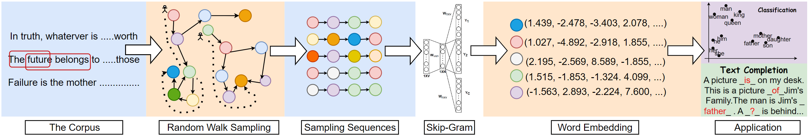
Figure 1: The overall framework for Word-Graph2vec algorithm.

3.2.1 Generate word co-occurrence graph

A textual document is presented as a word co-occurrence graph that corresponds to a weighted directed graph whose vertices represent unique words, whose edges represent co-occurrence between the words, and whose edge direction represents word order. An example of graph creation is given in Figure 2(a). The source text is an extract of a sentence from Philip Dormer Stanhope’s letter, “In truth, whatever is worth doing at all, is worth doing well; and nothing can be done well without attention." Figure 2(b) corresponds to the resulting weighted directed graph where each vertex represents a unique word, and each edge is a co-occurrence of the two words.

Weight on edges: The number of simultaneous occurrences of these two words in the text is used as the weight on edge. A weighted adjacency matrix $W$ is used to store the edge weights, and $W_{v,x}$ is the weight from node $v$ to node $x$.

$$W_{v,x}=\sum co\mbox{-}occurrence(v,x)$$ (1)

where $co\mbox{-}occurrence(v,x)$ is the number of times that the words $v$ and $x$ appear together from left to right in the same order.

Weight on nodes: The weight of the node is used to determine the sampling times in the random walk process. We take probability $PW_{v}$ as a representation of the importance of the word $v$ in the whole corpus, that is, the weight of nodes in the graph. This paper uses the terms frequency(TF) and inverse document probability(TF-IDF) to set the word weights $PW$.

(a) An example sentence. A solid arrow represents a new directed edge while a dashed arrow an already existing one in the graph. The edges are drawn from or to word “doing".

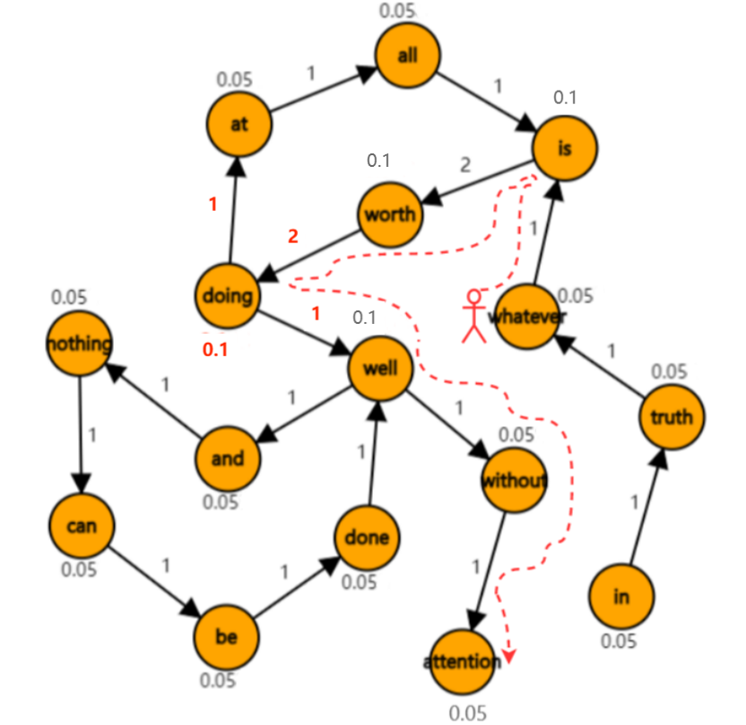
(b) The word co-occurrence graph. The red dotted line describes a random walk with “whatever" as the starting node and “attention” as the endding node.

Figure 2: An example of word co-occurrence graph creating from a sentence in Philip Dormer Stanhope’s letter.

3.2.2 Sampling word sequences by random walk

This random walk sampling process [16] iteratively explores the global structure network of the object to estimate the proximity between two nodes. Generate a random walk from the current node, and select the random neighbors of the current node as a candidate based on the transition probability on the word co-occurrence graph.

First, the different nodes, as distinct from the same selection probability for graph embedding, should have different probabilities to be selected as the starting point. We use the probability sampling method based on the word weight is applied to select the rooted node. For example, the sampling times of node $v$ as the starting node are shown in Equ 2:

$$number\_walks(v)=\left\lfloor total\_walks\times PW_{v}\right\rfloor$$ (2)

Where $total\_walks$ is the total number of random walk sampling, and $PW_{v}$ is the weight of word $v$.

Second, considering the shuttle between two kinds of graph similarities (homophily and structural equivalence), Node2vec [3] is selected as the graph sampling approach. Then, according to the the $2^{nd}$ order random walk transfer probability of the Node2vec model, the random neighbours of the current node is selected as the candidate node. The sampling sequence of a node is determined by simulating several biased random walks of fixed length $l$.

3.2.3 Learning embedding by Skip-Gram Model

After obtaining a much smaller set of walking sequences compared to the original corpus, we used the Skip-Gram model to learn the final word embedding.

3.3 Word-Graph2vec Algorithm

Word-Graph2vec algorithm is presented in Algorithm 1.

1

2Input: A processed corpus $C$, The number of sampling $n$, Walk length $l$, $p$, $q$ Context size $k$, Dimension $d$

3 Output: Word vector representations $\Phi$

41:  $W\leftarrow\emptyset$ // Adjacency Matrix ;

52:  $PW\leftarrow\emptyset$ // Weight on nodes ;

6

73:  for $i=1$ to $Size(C)$ do

8       for $word$ to $C_{i}$ do

9             $W_{word,word+1}\leftarrow W_{word,word+1}+1$  $PW_{word}\leftarrow PW_{word}+1$  

10      

11

124:  $\pi$ $\leftarrow$ PreprocessModifiedWeights$(W,p,q)$ ;

13

145:  $G^{\prime}=(V,E,\pi,PW)$;

15

166:  $SC\leftarrow\emptyset$ // SC is the result set of random walk sampling.

177:  for all nodes $u\in V$ do

18       for $iter=1$ to $n\frac{PW_{u}}{\sum_{k}PW_{k}}$ do

19             $word\_sequence\leftarrow\emptyset$ RandomWalkSampleProcess $(G^{\prime},u,l)$;

20             Append $word\_sequence$ to $SC$

21      

228:  $\Phi$ = Skip-Gram$(k,d,SC)$;

239:  return $\Phi$;

24

Algorithm 1 Word-Graph2vec Algorithm

The algorithm first initializes variables (Lines 1-2). We scan all the corpus once and build the word co-occurrence graph (Lines 1-3). The adjacency matrix $W$ and node’s weight $PW$ have been calculated in this scanning. Line 4 is to calculate the transitive matrix using the $2^{nd}$ transfer probability formula provided by Node2vec. Line 6-7 introduces how to generate the word sequences $SC$ by traveling on the word co-occurrence graph. The node on the graph is scanned one by one, and the number of times in which each node is traversed as the rooted node is equal to $n\frac{PW_{u}}{\sum_{k}PW_{k}}$.

3.4 Time and Space Complexity Analysis.

Denoting N as the total corpus size and $V$ as the unique word vocabulary count. In  Word-Graph2vec, the training corpus for Skip-Gram is our sampling corpus whose size is nl, where n is the number of random walks and l is the walk length. The time complexity is reduced to $O(nllog(V))$, since $n$l is smaller than $N$ ($nl\approx 1.9e^{8}$ for both 1GB and 4GB data set).

As for the space complexity, Word-Graph2vec needs to store the word graph, the generated word corpus, and the final word embedding. So, the space complexity of the word graph is $O(m|V|)$, $m$ is the average degree of the graph; the space complexity of generated word corpus is $O(nl)$; the word embedding is $O(d|V|)$. Therefore, the space complexity of Word-Graph2vec is $O(m|V|+nl+d|V|)$.

4 Experimental Analysis

4.1 Experimental Setting

We use various data sets to test our approaches. The processed dataset information can be found in Table 1.

Text8 : Text8 [10] contains 100M processed Wikipedia characters created by changing the case to lower of the text and removing any character other than the 26 letters $a$ through $z$. Meanwhile, PyDictonary, as in the English language dictionary, Wordnet lexical database, and Enchant Spell Dictionary, is applied to filter the correct English words.

One billion words benchmark (1b words banchmark)  : This is a new benchmark corpus with nearly 1 billion words of training data, which is used to measure the progress of statistical language modeling.

Enlish Wikipedia data set (En-Wikipedia) : This is a word corpus of English articles collected from Wikipedia web pages.

Concatenating data set: To test the scalability of our approach, we also process several En-Wikipedia data sets successively as a single sequential data set. We use Con-En-Wikipedia-i to denote the concatenating data set with $i\mbox{-}th$ data sets merged together. By the way, Con-En-Wikipedia-2 is 16.4G, and Con-En-Wikipedia-3 is 24.6 G.

Table 1: Statistics of Datasets

Data sets	Size	$|\mathrm{V}|$	$|\mathrm{E}|$	Density
Text8	95.3M	135,317	3,920,065	0.02$\%$
1b words benchmark	2.51G	82,473	54,125,475	0.80$\%$
En-Wikipedia	8.22G	100,723	64,633,532	0.64$\%$

Baseline method: Word2vec and Fasttext are two standard methods for training static word embedding, so we use them as our baseline to compare with  Word-Graph2vec. For these two baselines, all parameters are the default values provided by the original function

All our experiments are conducted on a PC with a 1.60GHz Intel Core 5 Duo Processor, 8GB memory, and running Win10, and all algorithms are implemented in Python and C++. Meanwhile, instead of using Node2vec, the Pecanpy model [6], which uses cache optimized compact graph data structure and pre-computing/parallelization to improve the shortcomings of Node2vec, is applied in our experiment.

4.2 Evaluation Criteria

We adopted the three evaluation tasks mentioned in [14]: Categorization, Similarity, and Analogy, and we tested them with the method proposed in [5].

Categorization: The goal here is to restore word clusters to different categories. Therefore, the corresponding word embedding of all words in the data set are clustered, and the purity of the cluster is calculated according to the marked data set.

Similarity: This task requires calculating the cosine similarity of paired words calculated using word vectors and comparing it with the relevant human judgment similarity.

Analogy:The goal is to find a term $x$ for a given term $y$ so that $x:y$ is most like the sample relationship $a:b$. It requires predicting the degree to which the semantic relations between $x$ and $y$ are similar to those between $a$ and $b$.

The word similarity prediction effectiveness is measured with the help of Spearman’s rank correlation coefficient $\rho$ [11]. For the analogy and the concept categorization tasks, we report the accuracy [8] in predicting the reference word and that of the class, respectively .

4.3 Parameters Study

Study of P, Q: We explored the best combination of parameters $p$ and $q$ on $[(0.001,1),(1,1),(1,0.001)]$. Table 2 shows the evaluation results of the three tasks. It can be seen from the results that the $(p,q)$combination of $(1,0.001)$ can obtain better accuracy.

Node’s weight study: Table 2 shows a comparison of the evaluation results of word embedding obtained by setting various word weight. Method 1 (Pecanpy+TF) uses $TF$ value as the weight of the node; Method 2 (Pecanpy+TF-IDF) uses $TF\mbox{-}IDF$ value; Method 3 (Pecanpy) do not set the node’s weight. The results show that using TF-IDF to set weights is the best, so we will use this method in the following experiments.

Table 2: Evaluation results of different $p$ , $q$ combinations and word weight setting

Tasks	Data set	Different $(p,q)$ Combimations			Different Word Weight Setting Method
		$(0.001,1)$	$(1,1)$	$(1,0.001)$	Pecanpy+TF	Pecanpy+TF-IDF	Pecanpy
Categorization Tasks (Accuracy*100)	BLESS	48.0	59.5	66.0	60.5	61.0	60.0
	Battig	25.1	30.0	32.2	32.1	34.3	30.1
Word Similarity (Spearman’s $\rho$ *100)	MEN	37.7	52.4	56.0	54.5	54.4	54.1
	SimLex999	20.6	18.1	21.5	21.3	21.7	20.4
Word Anology (Accuracy(P@1)*100)	MSR	4.0	15.7	11.9	12.9	12.3	12.1
	SemEval2012_2	8.4	13.5	10.4	11.0	11.5	10.3

Due to space limitations, we have only reported test results for some important parameters. Our final experiment used the best performing values for each parameter in the test.

4.4 Accuracy Experiments

We compared the performance of Word-Graph2vec, Word2vec, and FastText on three tasks. Table 3 show the experimental results of the categorization task, word similarity task and word analogy task. The experimental results show that: (i) On the three tasks, the quality of word embedding trained by Word-Graph2vec, Word2vec, and FastText will improve with the increased data set. We can see that the performance of Word-Graph2vec is gradually close to Word2vec and FastText, or even better. This shows that a random walk has a certain probability to capture marginal words that appear relatively few times. Thus, this makes the sampled corpus closer to the real text and even can follow the similar word’s distribution in advance. Moreover, this may be the reason to explain that the word embedding obtained by Word-Graph2vec performs better in some test tasks.

Table 3: Precision Experiments Results

Tasks		Categorization Tasks		Word Similarity		Word Anology
Datasets	Method	Accuracy*100		Spearman’s $\rho$ *100		Accuracy(P@1)*100
		BLESS	Battig	MEN	SimLex999	MSR	SemEval2012_2
Text8	Word2vec	58.0	35.2	63.0	26.3	27.6	13.2
	FastText	50.5	36.2	61.1	27.5	41.4	10.1
	Word-Graph2vec	66.0	32.2	56.0	21.5	11.9	10.4
1b Words Benchmark	Word2vec	77.0	30.8	68.6	33.0	34.8	13.9
	FastText	72.5	32.3	70.0	30.3	37.5	12.2
	Word-Graph2vec	83.5	31.6	70.1	31.6	24.8	15.7
En-Wikipedia	Word2vec	70.5	35.4	67.7	28.6	30.8	13.8
	FastText	77.0	37.3	69.0	28.4	42.8	15.6
	Word-Graph2vec	83.5	36.5	66.5	29.7	28.8	15.9

4.5 Efficiency of proposed algorithm

In order to observe the time trend more intuitively, we generated two more extensive data sets (Con-En-Wikipedia-1, 16.4G; Con-En-Wikipedia-2, 24.6G) for testing using the En-Wikipedia. As shown in Figure 3, we have plotted the experimental results on four data sets of different sizes (2.51G, 8.22G, 16.4G, 24.6G) into time curves (including 1b Words Benchmark and En-Wikipedia). Figure 3 indicates that the runtime of Word2vec and FastText increase almost linearly. But Word-Graph2vec ’s runtime increases slowly (the slight increase of runtime is due to loading the word corpus).

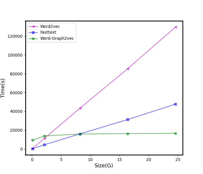
Figure 3: Times (h) vs. Size (G)

5 Conclusion

We propose the Word-Graph2vec algorithm to improve the performance of word embedding, which converts the large corpus into a word co-occurrence graph, then takes the word sequence samples from this graph by randomly walking and trains the word embedding on these sampling corpora in the end. We argue that due to the stable vocabulary, relative idioms, and fixed expressions in English, the size and density of the word co-occurrence graph change slightly with the increase of the training corpus. Thus, Word-Graph2vec has a stable runtime on the large-scale data set, and its performance advantage becomes more and more obvious with the growth of the training corpus. Experimental results show that the proposed algorithm outperforms traditional Word2vec in terms of efficiency and two-three times than FastText.

6 Acknowledgment

The authors acknowledge funding from 2023 Special Fund for Science and Technology Innovation Strategy of Guangdong Province (Science and Technology Innovation Cultivation of College Students), the Shenzhen High-Level Hospital Construction Fund (4001020), and the Shenzhen Science and Technology Innovation Committee Funds (JSGG20220919091404008, JCYJ20190812171807146).

References

- [1] Blanco, R., Lioma, C.: Graph-based term weighting for information retrieval. Information retrieval 15(1), 54–92 (2012)
- [2] Faruqui, M., Dodge, J., Jauhar, S.K., Dyer, C., Hovy, E., Smith, N.A.: Retrofitting word vectors to semantic lexicons. arXiv preprint arXiv:1411.4166 (2014)
- [3] Grover, A., Leskovec, J.: node2vec: Scalable feature learning for networks. In: Proceedings of the 22nd ACM SIGKDD international conference on Knowledge discovery and data mining. pp. 855–864 (2016)
- [4] Hassan, S., Mihalcea, R., Banea, C.: Random walk term weighting for improved text classification. International Journal of Semantic Computing 1(04), 421–439 (2007)
- [5] Jastrzebski, S., Leśniak, D., Czarnecki, W.M.: How to evaluate word embeddings? on importance of data efficiency and simple supervised tasks. arXiv preprint arXiv:1702.02170 (2017)
- [6] Liu, R., Krishnan, A.: Pecanpy: a fast, efficient and parallelized python implementation of node2vec. Bioinformatics 37(19), 3377–3379 (2021)
- [7] Manning, C., Raghavan, P., Schütze, H.: Introduction to information retrieval. Natural Language Engineering 16(1), 100–103 (2010)
- [8] Metz, C.E.: Basic principles of roc analysis. In: Seminars in nuclear medicine. vol. 8, pp. 283–298. Elsevier (1978)
- [9] Mikolov, T., Chen, K., Corrado, G., Dean, J.: Efficient estimation of word representations in vector space. arXiv preprint arXiv:1301.3781 (2013)
- [10] MultiMedia, L.: Large text compression benchmark (2009)
- [11] Myers, J.L., Well, A.D., Lorch Jr, R.F.: Research design and statistical analysis. Routledge (2013)
- [12] Pennington, J., Socher, R., Manning, C.D.: Glove: Global vectors for word representation. In: Proceedings of the 2014 conference on empirical methods in natural language processing (EMNLP). pp. 1532–1543 (2014)
- [13] Perozzi, B., Al-Rfou, R., Skiena, S.: Deepwalk: Online learning of social representations. In: Proceedings of the 20th ACM SIGKDD international conference on Knowledge discovery and data mining. pp. 701–710 (2014)
- [14] Schnabel, T., Labutov, I., Mimno, D., Joachims, T.: Evaluation methods for unsupervised word embeddings. In: Proceedings of the 2015 conference on empirical methods in natural language processing. pp. 298–307 (2015)
- [15] Si, Y., Wang, J., Xu, H., Roberts, K.: Enhancing clinical concept extraction with contextual embeddings. Journal of the American Medical Informatics Association 26(11), 1297–1304 (2019)
- [16] Wang, Z.W., Wang, S.K., Wan, B.T., Song, W.W.: A novel multi-label classification algorithm based on k-nearest neighbor and random walk. International Journal of Distributed Sensor Networks 16(3), 1550147720911892 (2020)