One-Shot Distributed Source Simulation: As Quantum as it Can Get

Abstract

Distributed source simulation is the task where two (or more) parties share some correlated randomness and use local operations and no communication to convert this into some target correlation. Wyner’s seminal result showed that asymptotically the rate of uniform shared randomness needed for this task is given by a mutual information induced measure, now referred to as Wyner’s common information. This asymptotic result was extended by Hayashi in the quantum setting to separable states, the largest class of states for which this task can be performed. In this work we characterize this task in the one-shot setting using the smooth entropy framework. We do this by introducing one-shot operational quantities and correlation measures that characterize them. We establish asymptotic equipartition properties for our correlation measures thereby recovering, and in fact strengthening, the aforementioned asymptotic results. In doing so, we consider technical points in one-shot network information theory and generalize the support lemma to the classical-quantum setting. We also introduce entanglement versions of the distributed source simulation task and determine bounds in this setting via quantum embezzling.

I Introduction

At the core of information theory is the notion of correlation. This is present even in Shannon’s initial work, as one can view both source and channel coding as the limits of establishing perfect correlation between inputs and outputs [1]. Another task where correlation plays a central role is that of distributed source simulation, which asks how much correlation must be provided to two spatially-separated and non-interacting parties so that they can generate a target joint distribution $p_{XY}$ up to some tolerated error $\varepsilon$ (see Fig. 1). It was established by Wyner that when the tolerated error is expressed in terms of regularized relative entropy, the rate of generating i.i.d. copies of $p_{XZ}$ is given by

$$R= \min_{q_{XYZ}:q_{XZ}=p_{XZ}\,\&\,X-Y-Z}I(XZ{\,:\,}Y)_{q}$$ (1)

$$:= \,C(X{\,:\,}Z)_{p}\ ,$$

where $X-Y-Z$ denotes a short Markov chain [2]. The correlation measure on the right hand side is often referred to as ‘Wyner’s common information.’ The achievability of this result was established by Wyner’s introduction of what is now referred to as a soft-covering lemma.

Figure 1: The general structure of distributed classical source simulation. The seed is copied and distributed, forming a source of shared randomness between Alice and Bob. Then Alice and Bob apply local maps to construct an output distribution $\widehat{q}_{XZ}$, which should approximate the target distribution $p_{XZ}$.

Since Wyner’s initial work, which was inspired by prior work by Gács-Körner [3] and Witsenhausen [4], many variations of common information and refinements of distributed source simulation have been considered. Liu et al. extended distributed source simulation to multipartite joint distributions [5]. Yu and Tan considered Rényi divergences and total variation as measures of error, which in particular led to them establishing a strong converse under the total variation measure [6, 7]. Winter extended to the case where there is an eavesdropper, the adversarial setting, so that it relates to key distillation [8]. Chitambar et al. compared this adversarial setting to the collaborative alternative [9]. Moreover, Chitambar et al. related the adversarial setting to quantum entanglement manipulations [10, 11] at one point using the Gács-Körner common information [3], which also is relevant in round complexity of state transformations [12]. Cuff established a general tradeoff region between Wyner common information and the classical reverse Shannon theorem when simulating a classical channel [13]. There is also the related problem of exact common information introduced by Kumar et al. which considers that the target state $p_{XY}^{\otimes n}$ is exactly constructed but allows for variable-length codes [14]. It was established by Yu and Tan that the exact common information corresponds to the common information with the error measured in terms of the max-divergence [15]. Furthermore, the soft-covering lemma used for achievability was established for error measured in total variation by Hayashi [16] and Cuff [17] and in the one-shot setting for Rényi divergence error by Yu and Tan [18]. We refer the reader to Yu and Tan’s recent monograph for further details on the history of common information in the classical setting [19].

However, the bulk of this previous research has been restricted to the classical common information. In the quantum setting, there are fundamental differences. Indeed, one of the key features of quantum mechanics, and consequently resources of quantum information theory, is quantum entanglement, which is a form of correlation that classical systems do not admit [20]. One way entanglement has been presented is as a quantum analogue of perfect correlation, the latter being the underlying resource in distributed classical source simulation. However, it has been shown that one cannot freely transform entanglement by local processing like one can with classical shared randomness without communication between the distributed parties [21]. That is to say, the fully entangled equivalent of distributed source simulation is not possible. Moreover, distributed parties who can only communicate classically cannot generate entanglement from shared randomness [22], and so the task cannot be extended to using the shared randomness to generate an entangled state.

Nonetheless, there is still space for a quantum extension. Specifically, the set of quantum distributions which are not entangled are the separable states, which is a strict superset of classical distributions. Separable states can be decomposed into a convex combination of product (quantum) distributions and consequently should be able to be simulated in a distributed manner. Indeed, Hayashi extended Wyner’s result to all separable states in terms of trace norm error [23]. In doing so, he introduced a novel covering lemma for quantum states that does not presume i.i.d. structure, i.e. is a one-shot characterization, although a quantum covering lemma with i.i.d. structure had been previously introduced by Ahlswede and Winter for considering different tasks [24].

This has remained the state of the quantum extension of Wyner’s common information for more than a decade. However, very recently there has been improvements upon the quantum one-shot soft-covering lemma. In particular, its error exponents have been characterized in terms of Rényi mutual information measures [25] and its second-order asymptotics were established via a characterization in terms of hypothesis testing mutual information [26]. This would suggest the possibility of establishing a one-shot version of Wyner’s common information for separable states which recovers Hayashi’s asymptotic extension.

Summary of Results

In this work, we extend distributed source simulation and Wyner’s common information to the one-shot quantum setting for separable states using the smooth entropy framework. In doing so, we introduce new measures of operational tasks $C^{\varepsilon}_{F},C^{\varepsilon}_{U,F},\widetilde{C}^{\varepsilon}_{F}$, where $C^{\varepsilon}_{U,F}$ is the one-shot version of Wyner’s quantity restricted to uniform shared randomness, $C^{\varepsilon}_{F}$ relaxes the requirement that the randomness be uniform, and $\widetilde{C}^{\varepsilon}_{F}$ allows one to distribute entangled states that are indistinguishable from a Markov chain. We introduce new one-shot correlation measures to extend Wyner’s common information. Specifically, we introduce measures based on the max mutual information [27, 28] $C^{\varepsilon}_{\max}$,$\widetilde{C}^{\varepsilon}_{\max}$ as well as one induced by the hypothesis testing divergence, $C^{\varepsilon}_{h}$. We establish achievability and converse bounds on the one-shot distributed-source simulation and related tasks in terms of these measures which hold in general if the state is separable.

Theorem.

(One-Shot Distributed Source Simulation Bounds) Let $\varepsilon\in(0,1)$. Let $\rho_{AC}\in\mathrm{D}(A\otimes C)$ such that $\|\rho-\widetilde{\rho}\|_{1}\leq\varepsilon$ for some separable state $\widetilde{\rho}_{AC}$. Let $\varepsilon_{1},\varepsilon_{2}\in(0,1)$ satisfy $2\varepsilon_{1}+\varepsilon_{2}<\varepsilon$. Then,

$$C^{\sqrt{\varepsilon}}_{\max}(A{\,:\,}C)_{\rho} \leq C^{\varepsilon}_{F}$$

$$\leq C^{\varepsilon}_{U,F}\leq C^{\varepsilon_{1}}_{\max}(A{\,:\,}C)_{\rho}+\kappa(\varepsilon_{2})\ ,$$

where $\kappa(\varepsilon_{2})$ is a constant that scales as $o(n)$ for $\rho_{AC}^{\otimes n}$.

Theorem.

(Variations of Distributed Source Simulation Bounds) Let $\rho_{AC}$ be a separable state. If $\delta\in(0,\varepsilon)$ and $\eta\in(\frac{7}{8}\varepsilon,\varepsilon)$, then

$$\widetilde{C}^{\sqrt{\varepsilon}}_{\max}(A{\,:\,}C)_{\rho}\leq \widetilde{C}^{\varepsilon}_{F}(A{\,:\,}C)_{\rho}\leq\widetilde{C}^{\sqrt{\varepsilon-\eta}}_{\max}(A{\,:\,}C)_{\rho}+o(n)\ ,$$

or if $\delta^{\prime}\in(0,1-\varepsilon)$,

$$\widetilde{C}_{h}^{1-\varepsilon-\delta^{\prime}}(A{\,:\,}C)_{\rho}+o(n)\leq \widetilde{C}^{\varepsilon}_{F}(A{\,:\,}C)_{\rho}$$

$$\leq \widetilde{C}^{1-\varepsilon/8}_{h}(A{\,:\,}C)_{\rho}+o(n)\ ,$$

where $o(n)$ always represents a term that scales as $o(n)$ for $\rho_{AC}^{\otimes n}$.

We also establish a (weak) asymptotic equipartition property (AEP) for the correlation measures induced by max divergence for separable states, which do not follow from pre-existing asymptotic equipartition properties.

Theorem.

(AEP for One-Shot Wyner Common Information) Let $\rho_{AC}$ be separable. Then,

$$\lim_{\varepsilon\to 0}\lim_{n\to\infty}\left[\frac{1}{n}C^{\varepsilon}_{\max}(A^{n}{\,:\,}C^{n})_{\rho^{\otimes n}}\right]=C(A{\,:\,}C)_{\rho},$$

$$\lim_{\varepsilon\to 0}\lim_{n\to\infty}\left[\frac{1}{n}\widetilde{C}^{\varepsilon}_{\max}(A^{n}{\,:\,}C^{n})_{\rho^{\otimes n}}\right]=C(A{\,:\,}C)_{\rho}.$$

These AEPs allow us to not only recover Hayashi’s asymptotic extension of the Wyner common information, but establish something stronger which says that even if the source were not uniform or we allowed entanglement assistance but restricted to be approximately indistinguishable from a Markov chain, asymptotically these all achieve the same rate if the error is required to go to zero.

Theorem.

(All Variations Have Same Vanishing Error Rate)

$$C(A{\,:\,}C)_{\rho}= \lim_{\varepsilon\to 0}\lim_{n\to\infty}\left[\frac{1}{n}C^{\varepsilon}_{F}(A^{n}{\,:\,}C^{n})_{\rho^{\otimes n}}\right]$$

$$= \lim_{\varepsilon\to 0}\lim_{n\to\infty}\left[\frac{1}{n}C^{\varepsilon}_{U,F}(A^{n}{\,:\,}C^{n})_{\rho^{\otimes n}}\right]$$

$$= \lim_{\varepsilon\to 0}\lim_{n\to\infty}\left[\frac{1}{n}\widetilde{C}^{\varepsilon}_{F}(A^{n}{\,:\,}C^{n})_{\rho^{\otimes n}}\right]\ .$$

We also show how all the stated results extend beyond bipartite setting.

Finally, as these results cannot be extended to an entangled setting, we present entangled equivalents: ‘embezzling source simulation’ and a variation that allows for shared randomness. Both versions use embezzlement [29] to simulate the target state (See Fig. 2). In particular, we establish nearly tight upper and lower bounds in the case shared randomness is included.

Theorem.

Let $\rho\in\mathrm{D}(A\otimes C)$ and $\varepsilon\in[0,1)$. Then

$$\log(\mathrm{Ent}^{\varepsilon}_{A:C}(\rho))\leq C^{\varepsilon}_{SREE,S}(A{\,:\,}C)_{\rho}$$

$$\leq \frac{1}{\varepsilon}\log(\mathrm{Ent}_{A:C}(\rho))\ .$$

Moreover, both the lower bound and upper bound can be shown to be nearly tight while.

(a) Embezzling Source Simulation

(b) Entangled Source Simulation

Figure 2: Entangled state versions of distributed source simulation. Grey lines represent allowed correlations of either classical or quantum mechanical nature. (b) Embezzling source simulation where the auxiliary state is required to be output approximately decoupled from the simulated state. (c) Entangled Source Simulation where the auxiliary system may be arbitrarily correlated with the target distribution. This in particular allows for the use of classical correlation.

In establishing these listed results, we establish technical tools which may be of independent interest or use. We establish a generalization of the support lemma (Lemma 5) so as to establish cardinality bounds, which could be of use in other quantum settings with an auxiliary classical random variable. We discuss the difficulty of using one-shot measures induced by hypothesis testing when an auxiliary random variable is used, which we expect is relevant in other quantum network settings in the smooth entropy framework as well. We also prove various properties of one-shot mutual informations which exemplify the importance in choosing which one-shot mutual information one uses. In particular, we establish a property of max mutual information as originally defined in [27] that allows for straightforward cardinality bounds of an auxiliary classical random variable, but the alternatives discussed in [28] do not satisfy the same property.

Organization of the Paper

The rest of the paper is organized as follows. In Section II we establish basic notation used throughout this work. In Section III we present the necessary background on one-shot information measures. In Section LABEL:sec:one-shot-dss we introduce one-shot distributed source simulation, its variants, and its impossibility for entangled states. In Section IV, we introduce the one-shot correlation measures to capture distributed source simulation, the smooth max common information, and its variants. We also establish basic properties of these measures. In particular, we straightforwardly generalize the support lemma so as to establish cardinality bounds on these measures and show that there are cases where these measures are NP-hard to compute. In Section V we establish achievability for distributed source simulation and its variants in terms of their respective measures by modifying the one-shot soft-covering results of [26] to be in terms of max mutual information. In Section VI we establish converses for distributed source simulation and its variants in terms of their one-shot correlation measures. This along with the previous section establishes tight (to first order) characterization of these tasks in terms of smooth mutual information quantities. In Section VII, we establish weak asymptotic equipartition properties (AEPs) for our correlation measures, which do not simply follow from previous results. By establishing this weak AEP, we are able to both recover Hayashi’s asymptotic extension of Wyner common information as well as generalize it. In Section VIII, we explain how these results are straightforward to generalize to source simulation of more than 2 parties and clarify certain properties in this setting noted in [5]. In Section IX we present the entangled state versions of distributed source simulation and establish bounds on the resources for this task. Finally, in Section X, we re-summarize what we have presented and discuss avenues for future work.

II Notation

Our notation largely follows standard texts to which we refer the reader for further details [22, 30]. We will denote finite alphabets by calligraphic roman letters at the end of the alphabet, e.g. $\mathcal{X},\mathcal{Y},...$. The probability simplex over finite alphabet $\mathcal{X}$ is denoted $\mathcal{P}(\mathcal{X})$. We talk of complex Euclidean spaces (CESs), equivalently finite Hilbert spaces, denoted by capital roman letters, e.g. $A\equiv\mathbb{C}^{|\mathcal{X}|}$. Given a CES $A$, we define the following classes of operators. The space of endomorphisms is denoted $\mathrm{L}(A)$. The space of Hermitian operators is $\mathrm{Herm}(A)\equiv\{X\in\mathrm{L}(A):X=X^{\ast}\}$ where $\cdot^{\ast}$ is the conjugate transpose. The space of positive semidefinite operators is $\mathrm{Pos}(A)\equiv\{X^{\ast}X:X\in\mathrm{L}(A)\}$, where we remind the reader $X\in\mathrm{Pos}(A)$ if and only if all of the eigenvalues are non-negative. We will often use $P,Q$ to denote generic positive semidefinite operators.

Quantum States

The space of quantum states, referred to as density matrices is $\mathrm{D}(A)\equiv\{\rho\in\mathrm{Pos}(A):\Tr(\rho)=1\}$, where $\Tr(\cdot)$ is the trace. Often times we will have density matrices defined on tensor product spaces, so we will add subscripts to the state to specify, e.g. $\rho_{AB}\in\mathrm{D}(A\otimes B)$. We say a state $\rho_{A}$ is pure if there exists a vector $\ket{\psi}\in A$ such that $\rho_{A}=\outerproduct{\psi}{\psi}$. A quantum state is classical if it is diagonal in the standard basis, e.g. $\rho=\sum_{x\in\Sigma}p(x)E_{x,x}$ where $p\in\mathcal{P}(\Sigma)$ and $\{E_{x,y}\}_{x,y\in\Sigma}$ form the standard basis for $\mathrm{L}(X)$. We denote classical registers with capital roman letters at the end of the alphabet, e.g. $X,Y,...$ to help distinguish from quantum states. A classical-quantum (CQ) state has the following convenient decomposition: $\rho_{XB}=\sum_{x\in\mathcal{X}}p(x)\outerproduct{x}{x}\otimes\rho_{B}^{x}$, where $p\in\mathcal{P}(\mathcal{X})$ and $\{\rho_{B}^{x}\}_{x\in\mathcal{X}}$ are referred to as the conditional states. The space of sub-normalized states is given by $\mathrm{D}_{\leq}(A)\equiv\{\rho\in\mathrm{Pos}(A):\Tr(\rho)\leq 1\}$.

As alluded to in the introduction, quantum states can be partitioned into states that are and aren’t entangled, which are known as separable. A ‘bipartite’ quantum state $\rho\in\mathrm{D}(A\otimes B)$ is separable if and only if there exists a finite alphabet $\mathcal{X}$, probability distribution $p\in\mathcal{P}(\mathcal{X})$, and sets of density matrices $\{\sigma_{A}^{x}\}_{x\in\mathcal{X}}\subset\mathrm{D}(A),\{\tau_{B}^{x}\}_{x\in\mathcal{X}}\subset\mathrm{D}(B)$ such that

$$\rho=\sum_{x\in\mathcal{X}}p(x)\sigma_{A}^{x}\otimes\tau_{B}^{x}\ .$$ (2)

Any state that is not separable is entangled. We denote the space of separable states in $\mathrm{D}(A\otimes C)$ as $\mathrm{Sep}\mathrm{D}(A{\,:\,}C)$.

Quantum Channels

A map $\mathcal{E}:\mathrm{L}(A)\to\mathrm{L}(B)$ is a quantum channel, $\mathcal{E}\in\mathrm{C}(A,B)$, if it is a completely positive (CP) and trace preserving (TP) map. A particularly important class of channels for this work are the classical-to-quantum or preparation channels. Given CESs $A\equiv\mathbb{C}^{|\mathcal{X}|},B\equiv\mathbb{C}^{|\mathcal{Y}|}$, a preparation channel $\mathcal{E}_{\mathrm{prep}}$ may be defined by its action

$$\mathcal{E}_{\mathrm{prep}}(W):=\sum_{x\in\mathcal{X}}\bra{x}W\ket{x}\rho_{B}^{x}\ ,$$

where $W\in\mathrm{L}(A)$ and $\{\rho_{B}^{x}\}_{x\in\mathcal{X}}\subset\mathrm{D}(B)$. This means the channel projects the input into the standard basis and then prepares a state dependent on the outcome, i.e. if given $\outerproduct{x}{x}$, it prepares $\rho_{B}^{x}$, hence its name.

Metrics on States

Lastly, we consider two metrics on states. The first is the trace distance, which is the quantum generalization of the total variation in the sense that it captures the distinguishability between the two quantum states.

Definition 1.

Given $\rho,\sigma\in\mathrm{D}(A)$, the trace distance is

$$\mathrm{TD}(\rho,\sigma):=\frac{1}{2}\|X-Y\|_{1}\ ,$$

where $\|\cdot\|_{1}$ is the Schatten one-norm.

We will also consider the purified distance $P(\cdot,\cdot)$ which we refer the reader to [31] for detailed information. For our purposes it will be sufficient to note that for $\rho,\sigma\in\mathrm{D}(A)$,

$$\mathrm{TD}(\rho,\sigma)\leq P(\rho,\sigma)\leq\sqrt{2\mathrm{TD}(\rho,\sigma)}\ .$$ (3)

For the reader’s intuition we note that the purified distance is greater than the trace distance because it operationally measures the maximal distinguishability between purifications of $\rho,\sigma$ rather than the distinguishability of the states themselves. We also define the following equivalences for notational convenience:

$$P(\rho,\sigma)\leq\varepsilon\Leftrightarrow\rho\approx_{\varepsilon}\sigma$$ (4)

$$2\mathrm{TD}(\rho,\sigma)\leq\varepsilon\Leftrightarrow\rho\approx_{\varepsilon}^{\mathrm{TD}}\sigma$$ (5)

Lastly, we note, as they are metrics, they act as good distance measures on quantum states. As such, we can use them to measure the distance between a state and the set of separable states, which will be useful later.

Definition 2.

For $\rho_{AB}\in\mathrm{D}(A\otimes B)$, the trace distance of entanglement is defined as

$$E_{T}(A{\,:\,}B)_{\rho}:=\inf_{\sigma_{AB}\in\mathrm{Sep}\mathrm{D}(A{\,:\,}B)}\mathrm{TD}(\rho,\sigma)\ ,$$

and the purified distance of entanglement, $E_{P}(A{\,:\,}C)_{\rho}$, is defined identically with $\mathrm{TD}(\cdot,\cdot)$ replaced with the purified distance $P(\cdot,\cdot)$.

III One-Shot Entropies and Information Measures

We now summarize the background on one-shot entropies and their relation to asymptotic entropies as necessary for this work. We note that a secondary aspect of this work is to highlight what it means to determine the ‘correct’ one-shot mutual information in our setting as there are a myriad of them and because the previous work [26] initiates such a discussion. For this reason, this section is longer as it motivates why there are so many to begin with.

For $P,Q\in\mathrm{Pos}(A)$, the relative entropy is defined as

$$D(P||Q)=\Tr[P\log P]-\Tr[P\log Q]$$

when $\mathrm{Supp}(P)\subseteq\mathrm{Supp}(Q)$ and is otherwise infinite. This recovers the KL divergence if $P,Q$ are classical. From this definition one can extend the standard classical information quantities from the KL divergence to the quantum setting [30]. In particular, one can recover the many equivalent definitions of mutual information:

$$I(A{\,:\,}B)_{\rho}:= D(\rho_{AB}||\rho_{A}\otimes\rho_{B})$$ (6)

$$= \min_{\sigma_{B}\in\mathrm{D}(B)}D(\rho_{AB}||\rho_{A}\otimes\sigma_{B})$$

$$= \min_{\begin{subarray}{c}\tau_{A}\in\mathrm{D}(A)\\ \sigma_{B}\in\mathrm{D}(B)\end{subarray}}D(\rho_{AB}||\tau_{A}\otimes\sigma_{B})\ .$$

However, in the one-shot setting there are more entropic measures to use. In the classical setting, this is predominantly handled by the information spectrum divergence [32]. In the quantum setting there are multiple options. While there is the extension of the information spectrum divergence [33],

$$D^{\varepsilon}_{s}(\rho||Q):=\sup_{\gamma\in\mathbb{R}}\{\Tr[\rho\{\rho\leq\exp(\gamma)Q\}]\leq\varepsilon\}\ ,$$ (7)

there is also the smooth entropy calculus which ‘smooths’ entropic quantities defined in terms of the quantum max-relative divergence and duality (See [31]). The max-relative divergence is defined as

$$D_{\max}(P||Q):=\inf\{\lambda\in\mathbb{R}:P\leq\exp(\gamma)Q\}\ .$$ (8)

One appealing property of the max-relative divergence is that it benefits from a particularly general data processing inequality (DPI).

Proposition 1.

For any CP map $\mathcal{E}$, $D_{\max}(\mathcal{E}(P)||\mathcal{E}(Q))\leq D_{\max}(P||Q)$.

Proof.

Let $\gamma^{\star}$ be the optimizer for $D_{\max}(P||Q)$. As $\mathcal{E}$ is CP, $P\leq\exp(\gamma^{\star})Q$ implies $\mathcal{E}(P)\leq\exp(\gamma^{\star})\mathcal{E}(Q)$. As $D_{\max}$ is defined as an infimum and we have just shown $\gamma^{\star}$ is feasible for $D_{\max}(\mathcal{E}(P)||\mathcal{E}(Q))$, this completes the proof. ∎

Just as mutual information is defined from relative entropy, the max mutual information is defined from the max divergence. However, in general the three equivalent definitions given in (6) are inequivalent for $D_{\max}$ and thus there are three possible max mutual informations.

Definition 3.

For $\rho_{AB}\in\mathrm{D}_{\leq}(A\otimes B)$,

$$I^{\uparrow\uparrow}_{\max}(A{\,:\,}B)_{\rho} :=D_{\max}(\rho_{AB}||\rho_{A}\otimes\rho_{B})$$ (9)

$$I^{\uparrow}_{\max}(A{\,:\,}B)_{\rho} :=\min_{\sigma_{B}\in\mathrm{D}(B)}D_{\max}(\rho_{AB}||\rho_{A}\otimes\sigma_{B})$$ (10)

$$I^{\downarrow}_{\max}(A{\,:\,}B)_{\rho} :=\min_{\begin{subarray}{c}\tau_{A}\in\mathrm{D}(A)\\ \sigma_{B}\in\mathrm{D}(B)\end{subarray}}D_{\max}(\rho_{AB}||\tau_{A}\otimes\sigma_{B})\ .$$ (11)

We note (10) was introduced in [35] while (9) and (11) were introduced in [28]. Our notation differs from both of these to make the relation

$$I^{\uparrow\uparrow}_{\max}\geq I^{\uparrow}_{\max}(A{\,:\,}B)\geq I^{\downarrow}_{\max}(A{\,:\,}B)\ ,$$

explicit and also to align with the notation of more recent work, namely [36]. Moreover, we note that we could have defined the one-shot mutual informations for any Rényi mutual information $\mathbb{I}(A{\,:\,}B)$ (any mutual information defined using a Rényi divergence [31]). Certain results in this work are presented in such a manner for generality.

It is presumably clear that in general $I^{\uparrow\uparrow}_{\max},I^{\uparrow}_{\max}$, and $I^{\downarrow}_{\max}$ could behave quite differently. Indeed, as we will see, there are certain properties that make $I^{\uparrow}_{\max}$ preferable for our purposes. Nonetheless, Ciganovic et al. [28] showed that when smoothed, over a large parameter range of smoothing, these measures become asymptotically equivalent. We summarize this in sufficient detail to introduce the notion of smoothed measures and introduce the result we will need later.

Definition 4.

Let $\rho_{AB}\in\mathrm{D}_{\leq}(A\otimes B)$ and $\varepsilon\in(0,1)$. Then

$$\mathcal{B}^{\varepsilon}(\rho):=\{\widetilde{\rho}\in\mathrm{D}_{\leq}(A\otimes B):P(\rho,\widetilde{\rho})\leq\varepsilon\}\ ,$$

where $P(\cdot,\cdot)$ is the purified distance metric.

Definition 5.

For $x\in\{\uparrow\uparrow,\uparrow,\downarrow\}$, the smoothed max-mutual information is

$$I_{\max}^{x,\varepsilon}(A{\,:\,}B)_{\rho}:=\min_{\widetilde{\rho}\in\mathcal{B}^{\varepsilon}(\rho)}I_{\max}^{x,\varepsilon}(A{\,:\,}B)_{\widetilde{\rho}}\ .$$

Lemma 1.

([28, Theorem 3]) Let $\rho_{AB}\in\mathrm{D}(A\otimes B)$, $\overline{\varepsilon}>0$, $\overline{\varepsilon}^{\prime}\geq 0$, then

$$I^{\uparrow\uparrow,\overline{\varepsilon}+2\sqrt{\overline{\varepsilon}}+\overline{\varepsilon}^{\prime}}_{\max}(A{\,:\,}B)_{\rho}\leq I^{\uparrow,\overline{\varepsilon}^{\prime}}_{\max}(A{\,:\,}B)_{\rho}+g(\overline{\varepsilon})\ ,$$

where

$$g(x):=\log(\frac{2(1-x)+3}{(1-x)(1-\sqrt{1-x^{2}}})\ .$$\end{lemma}),\begin{aligned} \{C^{\varepsilon}_{F},\widetilde{C}^{\varepsilon}_{F}\}\leq\widehat{C}_{F}\quad\&\quad C^{\varepsilon}_{F}\leq C^{\varepsilon}_{U,F}\ .\end{aligned}$$

Proof.

That $C^{\varepsilon}_{F}\leq C^{\varepsilon}_{U,F}$ follows from it being a more restricted optimization. That $\widetilde{C}^{\varepsilon}_{F}\leq\widehat{C}^{\varepsilon}_{F}$ is also because it is a more restricted optimization. That $C^{\varepsilon}_{F}\leq\widehat{C}^{\varepsilon}_{F}$ is because if $\widetilde{\rho}\approx_{\varepsilon}^{\mathrm{TD}}\rho$, then as trace norm monotonically decreases under partial trace,

$$\varepsilon\geq \|\Tr_{X}(\widetilde{\rho}-\rho_{A-X-C})\|_{1}$$

$$\geq \|\sum_{x}p(x)\widetilde{\rho}_{A}^{x}\otimes\widetilde{\rho}_{C}^{x}-\rho_{AC}\|_{1}\,\Rightarrow\widetilde{\rho}\sim_{\varepsilon}\rho\$$

where the implication is by definition of $\varepsilon$-simulation. This completes the proof. ∎

(a) Correlation of Formation, $C^{\varepsilon}_{F}$

(b) Secret EA Correlation of Formation, $\widetilde{C}^{\varepsilon}_{F}$

(c) Private Correlation of Formation, $\widehat{C}^{\varepsilon}_{F}$

Figure 3: The three correlation of formations and their corresponding tasks: (a) Correlation of formation captures the amount of randomness for distributed source simulation. (b) Secret entanglement-assisted correlation of formation captures the amount of broadcasted randomness needed such that there exists a set of (possibly entangled) states $\{\widetilde{\rho}_{AC}^{x}\}_{x\in\mathcal{X}}$ to distribute so that the entire output is approximately indistinguishable from a distributed source simulation implementation of the target state. (c) Private correlation of formation measures the amount of randomness needed for a distributed source simulation protocol so that if the randomness were to be leaked it would be approximately indistinguishable from an exact distributed source simulation of the target state with leaked classical information.

We stress in particular the following two points implicit in the above proposition. First, one would expect there are cases where the inequality $C^{\varepsilon}_{F}\leq\widehat{C}^{\varepsilon}_{F}$ is large because in $\widehat{C}^{\varepsilon}_{F}$ the distinguisher has access to the $X$ register. That is to say, in general one expects there to be a non-trivial difference between

$$\min_{\widetilde{\rho}_{A-X-C}}\left\|\Tr_{X}(\widetilde{\rho}_{A-X-C})-\rho_{AC}\right\|_{1}$$

and

$$\min_{\begin{subarray}{c}\widetilde{\rho}_{A-X-C}\\ \rho_{A-X-C}\end{subarray}}\sum_{x}\left\|\widetilde{p}(x)\widetilde{\rho}^{x}_{A}\otimes\widetilde{\rho}^{x}_{C}-p(x)\rho_{A}^{x}\otimes\rho_{C}^{x}\right\|_{1}\ .$$

Second, intuitively $C^{\varepsilon}_{F}$ and $\widetilde{C}^{\varepsilon}_{F}$ do not seem comparable as the resources allowed are fundamentally different. We now show this to be formally true by establishing the quantities are finite under different conditions. We begin with the following lemma that will be used extensively in this work.

Lemma 2.

A quantum state $\rho_{AC}\in\mathrm{D}(A\otimes C)$ has a Markov chain extension $\rho_{A-B-C}:\Tr_{B}\rho_{A-B-C}=\rho_{AC}$ if and only if $\rho_{AC}\in\mathrm{Sep}\mathrm{D}(A{\,:\,}C)$.

Proof.

We prove both directions.
($\Rightarrow$) Let $\rho_{AC}\in\mathrm{Sep}\mathrm{D}(A{\,:\,}C)$. Then by definition, $\rho_{AC}=\sum_{x}p(x)\rho_{A}^{x}\otimes\rho_{C}^{x}$ for some finite alphabet $\mathcal{X}$, $p\in\mathcal{P}(\mathcal{X})$, and sets of quantum states $\{\rho_{A}^{x}\}_{x\in\mathcal{X}}$, $\{\rho_{C}^{x}\}_{x\in\mathcal{X}}$. It follows $\sum_{x}p(x)\rho^{x}_{A}\otimes\outerproduct{x}{x}\otimes\rho^{x}_{C}$ is a QMC extension as $\mathcal{R}(\cdot):=\sum_{x}\Tr[\outerproduct{x}{x}\cdot]\rho^{x}_{C}\otimes\outerproduct{x}{x}$ and same idea for $\overline{\mathcal{R}}$.
($\Leftarrow$) If one has a QMC $\rho_{A-B-C}$, then by Theorem LABEL:thm:QMC-equivalences, $\rho_{A-B-C}=\bigoplus_{j\in\mathcal{J}}p(j)\rho_{Ab^{L}_{j}}\otimes\rho_{b^{R}_{j}C}$ where the $\rho_{Ab^{L}_{j}}$, $\rho^{b^{R}_{j}C}$ are density matrices on the respective subspaces. It follows

$$\Tr_{B}(\rho_{A-B-C})= \bigoplus_{j\in\mathcal{J}}p(j)\Tr_{b^{L}_{j}}(\rho_{Ab^{L}_{j}})\otimes\Tr_{b^{R}_{j}}(\rho_{b^{R}_{j}C})$$

$$= \sum_{j\in\mathcal{J}}p(j)\rho_{A}^{j}\otimes\rho_{C}^{j}\ \in\mathrm{Sep}(A{\,:\,}C)\ ,$$

where we have used that for $B=\oplus_{j\in\mathcal{J}}b^{L}_{j}\otimes b^{R}_{j}$, we may decompose $\Tr_{B}=\oplus_{j\in\mathcal{J}}\Tr_{b^{L}_{j}\otimes b^{R}_{j}}$ and then $\Tr_{b^{L}_{j}}\otimes\Tr_{b^{R}_{j}}$ will distribute across the tensor product of the states decomposition as is normal. This completes the proof. ∎

We also will make use of the following straightforward proposition.

Proposition 2.

For all $\delta\in(0,1)$, if there exists a QMC $\rho_{A-X-C}$, there exists $\widehat{\rho}_{A-\pi-C}$ such that $\rho_{AC}\approx_{\delta}^{\mathrm{TD}}\widehat{\rho}_{AC}$.

Proof.

Let $\rho_{A-X-C}=\sum_{x\in\mathcal{X}}p(x)\rho_{A}^{x}\otimes\outerproduct{x}{x}\otimes\rho^{x}_{C}$. Then there exists finite alphabet $\mathcal{X}^{\prime}$ and $\{k_{x}\}\subset\{0,...,|\mathcal{X}^{\prime}|\}$ such that $\sum_{x}k_{x}=|\mathcal{X}^{\prime}|$ and $\sum_{x\in\mathcal{X}}|k_{x}/|\mathcal{X}^{\prime}|-p(x)|\leq\delta$ since the rationals are dense in $[0,1]$. Define $\widetilde{\rho}_{A-\pi-C}=\frac{1}{X^{\prime}}\sum_{x^{\prime}\in\mathcal{X}^{\prime}}\rho^{f(x^{\prime})}_{A}\otimes\outerproduct{x^{\prime}}{x^{\prime}}\rho^{f(x^{\prime})}_{C}$ where $f:\mathcal{X}^{\prime}\to\mathcal{X}$ is such that for each $x\in\mathcal{X}$, it maps $k_{x}$ of the elements of $\mathcal{X}^{\prime}$ to that $x$. Note this means $\widetilde{\rho}_{A}^{x^{\prime}}=\rho_{A}^{f(x^{\prime})}$ for all $x^{\prime}\in\mathcal{X}^{\prime}$ not that we are actually indexing by $f(x^{\prime})$ which would erase information we need to preserve the Markov chain condition. It follows by our construction

$$\left\|\Tr_{X^{\prime}}(\widetilde{\rho}_{A-\pi-C})-\Tr_{X}(\rho_{A-X-C})\right\|_{1}$$

$$= \left\|\sum_{x\in\mathcal{X}}\frac{k_{x}}{|\mathcal{X}^{\prime}|}\rho^{x}_{A}\otimes\rho^{x}_{C}-\sum_{x\in\mathcal{X}}p(x)\rho^{x}_{A}\otimes\rho^{x}_{C}\right\|_{1}$$

$$\leq \left\|\sum_{x\in\mathcal{X}}\frac{k_{x}}{|\mathcal{X}^{\prime}|}\outerproduct{x}{x}^{\otimes 2}-\sum_{x}p(x)\outerproduct{x}{x}^{\otimes 2}\right\|_{1}$$

$$= \sum_{x}\left|\frac{k_{x}}{|\mathcal{X}^{\prime}|}-p(x)\right|\leq\delta\ ,$$

the first inequality uses the data-processing inequality for the one-norm and the preparation channels $\Phi_{1}(\cdot)=\Tr[\outerproduct{x}{x}\cdot]\rho^{x}_{A}$ and $\Phi_{2}(\cdot)=\Tr[\outerproduct{x}{x}\cdot]\rho^{x}_{C}$. ∎

Theorem 3.

Let $\rho\in\mathrm{D}(A\otimes C)$.

1. For $\varepsilon\in[0,1]$, $\widetilde{C}^{\varepsilon}_{F}(A{\,:\,}C),\widehat{C}^{\varepsilon}_{F}(A{\,:\,}C)$ are finite if and only if $\rho_{AC}\in\mathrm{Sep}\mathrm{D}(A{\,:\,}C)$.

2. In contrast, $C^{\varepsilon}_{F}(A{\,:\,}C)_{\rho}$ is finite if and only if $E_{T}(A{\,:\,}C)_{\rho}\leq 2\varepsilon$. Likewise, $C^{\varepsilon}_{U,F}(A{\,:\,}C)_{\rho}$ if and only if there exists $\delta\in(0,\varepsilon)$ such that $E_{T}(A{\,:\,}C)_{\rho}\leq 2(\varepsilon-\delta)$.

Proof.

We begin with Item 1. The only if direction is immediate because if there exists an appropriate QMC extension, then the state is separable by Lemma 2. Likewise, by Lemma 2, if $\rho_{AC}\in\mathrm{Sep}\mathrm{D}(A{\,:\,}C)$, there exists a QMC extension of $\rho_{AC}$, $\rho_{A-X-C}=\sum_{x}p(x)\rho^{x}_{A}\otimes\outerproduct{x}{x}\otimes\rho^{x}_{C}$ for some finite alphabet $\mathcal{X}$. This state is then feasible for $\widetilde{C}^{\varepsilon}_{F},\widehat{C}^{\varepsilon}_{F}$. Note none of this has relied on the choice of $\varepsilon$.

For $C^{\varepsilon}_{F}$, note that if $E_{T}(A{\,:\,}C)_{\rho}\leq 2\varepsilon$, there exists $\widetilde{\rho}\in\mathrm{Sep}\mathrm{D}(A{\,:\,}C)$ such that $\widetilde{\rho}\approx_{\varepsilon}^{\mathrm{TD}}\rho$. Then there exists a QMC extension of $\widetilde{\rho}_{AC}$ by Lemma 2 and this QMC extension satisfies $\widetilde{\rho}_{A-X-C}\sim_{\varepsilon}\rho_{AC}$. If no such state exists, then there is no QMC extension by Lemma 2. For the uniformity claim, note that if such a $\delta>0$ exists then by Proposition 2 we may do the same argument again. This completes the proof. ∎

Therefore we see $C^{\varepsilon}_{F}$ is a fundamentally distinct measure from $\widetilde{C}^{\varepsilon}_{F},\widehat{C}^{\varepsilon}_{F}$ as when they are finite is not even in agreement. We will discuss this further after we have introduced the one-shot correlation measures.

IV One-Shot Correlation Measures

As is standard in information theory, the ultimate goal is to establish bounds in terms of entropic quantities. In our case we would particularly like to bound the correlations of formations with entropic quantities that recover Wyner’s common information in the asymptotic limit. That is, our hope is to construct bounds in terms of an entropic quantity $\mathbb{C}^{?}$ that on i.i.d. inputs satisfies

$$\lim_{n\to\infty}\left[\frac{1}{n}\mathbb{C}^{?}(A^{n}{\,:\,}C^{n})_{\rho^{\otimes n}}\right]=\min_{A-X-C}I(AC{\,:\,}X)_{\rho}\ ,$$

where we note the right hand side is Wyner’s common information as per (1). Motivated by this end goal, we introduce the max common information, its smoothed versions, and establish certain properties of it on single copies of a state. In doing so we will present the generalized support lemma. Moreover, we introduce the hypothesis testing common information and show it satisfies the same wanted properties. We end the section by establishing that these introduced correlation measures act as one-shot converses to the distributed source simulation tasks.

We claim the natural one-shot extension of Wyner’s common information is the following.

Definition 6.

Given $\rho_{AC}\in\mathrm{D}(A{\,:\,}C)$, the Max Common information is

$$C_{\max}(A{\,:\,}C)_{\rho}:=\min_{A-X-C}I^{\uparrow}_{\max}(AC{\,:\,}X)_{\rho}\ .$$ (12)

There are three choices we should justify: (i) the restriction to a classical register, (ii) the minimization, and (iii) the choice of $I^{\uparrow}_{\max}$ rather than another version.

First we justify why we restrict to $A-X-C$ Markov chains in the above definition. We could of course argue it is because we are interested in an operational interpretation that will require the classical register. However, this restriction can be made without loss of generality for any mutual information that satisfies DPI as we now show.

Lemma 4.

Let $\rho_{ABC}$ be a $A-B-C$ Markov chain. Then there always exists a $A-X-C$ Markov chain $\rho_{AXC}^{\prime}$ such that $\rho_{AC}^{\prime}=\rho_{AC}$ and $\mathbb{I}^{x}(AC{\,:\,}B)_{\rho}\geq\mathbb{I}^{x}(AC{\,:\,}X)_{\rho^{\prime}}$, where $\mathbb{I}$ is any mutual information measure that satisfies data-processing and $x\in\{\uparrow\uparrow,\uparrow,\downarrow\}$ following Definition 3.

Proof.

We prove it for $\mathbb{I}^{\downarrow}(AC:X)$ case as it is then straightforward to see the same proof method will hold for the other cases. Let $\rho_{ABC}$ be a $A-B-C$ Markov chain. Then $\rho_{B}=\oplus_{x}p(x)\rho_{b^{L}_{x}}\otimes\rho_{b^{R}_{x}}$. Define the map $\mathcal{E}:B\to BX$ as $\mathcal{E}(\cdot)=\sum_{j}\Pi_{x}^{B}\cdot\Pi_{x}^{B}\otimes\outerproduct{x}{x}_{X}$ where $\{\Pi_{x}\}$ are the mutually orthogonal projectors onto the subspaces $b^{L}_{x}\otimes b^{R}_{x}$. Define $\rho_{ABXC}^{\prime}:=\mathcal{E}(\rho_{ABC})$. Then it follows

$$\mathbb{I}^{\downarrow}(AC:B)_{\rho}= \mathbb{D}(\rho_{ABC}||\tau_{AC}\otimes\sigma_{B})$$

$$\geq \mathbb{D}(\rho_{ABXC}^{\prime}||\tau_{AC}\otimes\sigma_{BX})$$

$$\geq \mathbb{D}(\rho_{AXC}^{\prime}||\tau_{AC}\otimes\sigma_{X})$$

$$\geq \min_{\begin{subarray}{c}\tau^{\prime}\in\mathrm{D}(AC)\\ \sigma^{\prime}\in\mathrm{D}(X)\end{subarray}}\mathbb{D}(\rho_{AXC}^{\prime}||\tau_{AC}^{\prime}\otimes\sigma_{X}^{\prime})$$

$$= \mathbb{I}^{\downarrow}(AC:X)_{\rho^{\prime}}\ ,$$

where the first inequality is DPI using $\mathcal{E}$, the second inequality is DPI using the partial trace on the $B$ space, and in both cases the map only acts on one side of conditioned tensor product, and the final is just re-minimizing. We can also guarantee $\sigma_{X}^{\prime}$ is classical by DPI and pinching on the computational basis. Moreover $\rho_{AXC}^{\prime}$ is $A-X-C$ Markov chain extension of $\rho_{AC}$ trivially as $\mathcal{E}$ never acted on the $AC$ spaces and its recovery maps are just state preparations maps, e.g. $x\mapsto\Tr_{b^{L}_{x}}(\rho^{Ab^{L}_{x}})$. This completes the proof. ∎

Remark 1.

It is worth noting why the above isn’t proven to be an equality. When one converts the $B$ register to a classical $X$ register, they destroy any entanglement between $A$ (resp. $C$) and $b^{L}_{x}$ (resp. $b^{R}_{x}$). To recover this entanglement, one needs to apply the recovery map, e.g.

$$\rho_{X}\to\rho_{B}\xrightarrow[]{\mathcal{R}}\rho_{BC}\xrightarrow[]{\overline{\mathcal{R}}}\rho_{ABC}\ .$$

However, to preserve the form of mutual information, you can only act on the $B$ space, so it is not possible to evaluate this directly.

This justifies the restriction to a classical register. To address the second and third question, we will need to introduce the generalized support lemma.

IV-A The Generalized Support Lemma

The convex cover method using the support lemma is a standard method in classical information theory for bounding the cardinality of an auxiliary variable [41, Appendix C]. This bounding is useful as then the space being optimized over is finite-dimensional and thus closed. Effectively the support lemma implies that if all the relevant constraints may be written as the expectation of a function over conditional distributions according to the auxiliary variable, then the auxiliary variable can be made finite. Our extension states the same but replacing conditional distributions with conditional states from an appropriate state space. This generalization is necessary for our purposes as we will need to consider a function of conditional states, appearing in Lemma 6, that does not reduce to functions of their spectra.

We begin by stating Carathéodory’s theorem of which the support lemma may be viewed as a corollary.

Proposition 3.

(Fenchel-Eggleston-Carathéodory) Any point in a convex closure of a connected compact set $\mathscr{R}\in\mathbb{R}^{d}$ can be represented as a convex combination of at most $d$ points in $\mathscr{R}$.

Now we present the general lemma.

Lemma 5.

(Generalized Support Lemma) Let $\mathcal{W}$ be an arbitrary set. Let the generalized state space $\mathscr{S}(A)$ be a connected, compact subset of $\mathrm{Pos}(A)$ and $\{\rho_{w}\}_{w\in\mathcal{W}}\subseteq\mathscr{S}(A)$ be a set of generalized conditional states. Let $\{f_{j}\}_{j\in[k]}\subset\mathscr{S}(A)\to\mathbb{R}$ be continuous. Then for any Borel measure $\mu$ of $\mathcal{W}$, there exists $q\in\mathcal{P}(\mathcal{W}^{\prime})$ where $|\mathcal{W}^{\prime}|\leq k$ and $\{\sigma_{w^{\prime}}\}_{w^{\prime}\in\mathcal{W}^{\prime}}\subset\mathscr{S}(A)$ such that

$$\int_{\mathcal{W}}f_{j}(\rho_{w})\mu(dW)=\sum_{w^{\prime}\in\mathcal{W}^{\prime}}f_{j}(\sigma_{w^{\prime}})q(w^{\prime})\ .$$

Proof.

Our proof is a direct extension of the proof given for the traditional support lemma by Csiszar and Körner [42, Lemma 15.4]. By assumption, $\mathscr{S}(A)$ is a compact, connected subset. By assumption each $f_{j}$ is continuous, so the image of $f_{j}(\rho)$ is both connected and compact. Define $F(\rho):=(f_{1}(\rho),...,f_{k}(\rho))$ and the set $\mathcal{R}:=\{F(\rho),\rho\in\mathscr{S}(A)\}$, which is connected and compact as product preserves these properties. Moreover, defining

$$r_{j}\equiv\int_{W}f_{j}(\rho_{w})\mu(dW)\quad\forall j\in[k]\ ,$$

we have $(r_{1},...,r_{k})$ is an element of the convex closure of $\mathcal{R}$. Therefore, applying Proposition 3, there exist $k$ points of $\mathcal{R}$, which we denote $\{F(\sigma_{j})\}_{j\in\mathcal{K}}$, along with a distribution $q\in\mathcal{P}([k])$ such that

$$(r_{1},...,r_{k})=\sum_{j\in[k]}q(j)F(\sigma_{j})\ .$$

By definition of $F(\rho)$, we can conclude $r_{j}=\sum_{j}q(i)f(\sigma_{i})$ for all $i\in[k]$. Letting $\mathcal{W}^{\prime}=[k]$ completes the proof. ∎

First, we note the reason we talk in terms of generalized state spaces that are subsets of the positive density matrices is that, for example, this would allow for cardinality bounds on subnormalized states which may be of use given smoothed measures. In fact, any closed convex subset of the (possibly subnormalized) density matrices would work, since it would be compact and all convex sets are (path-)connected. Moreover, the generalized state space may be the product space of closed convex subsets of the (possibly subnormalized) density matrices, since the product of connected, compact sets are also connected and compact, which is useful for network settings. Note you can also restrict to the support of some state space as needed.

We now can use this to bound the cardinality of the the max common information which will also explain why we chose $I^{\uparrow}_{\max}$. This relies on various technical lemmas about mutual informations which we relegate to an appendix and summarize here.

Lemma 6.

Let $\rho_{ABX}$ be classical on $X$. Then,

$$\exp(I^{\uparrow}_{\max}(AC{\,:\,}X)_{\rho})=\sum_{x}p_{x}\exp(D_{\max}(\rho_{AC}^{x}||\rho_{AC}))\ ,$$

where the right hand side is a continuous function over the state space restricted to $\rho_{AC}$’s support. Moreover, $I^{\uparrow\uparrow},I^{\downarrow}$ do not seem to satisfy such an averaging statement.

Proof.

One uses Corollary 2 in the appendix with the replacements $A\to AC$, $B\to\mathbb{C}$. To simplify the RHS term, note, as defined in the appendix, $I_{\max}(\rho_{AC\mathbb{C}}^{x}||\rho_{AC})=D_{\max}(\rho_{AC}^{x}||\rho_{AC})$ for each $x$. Finally taking an exponential gets the form in the lemma. That $I^{\uparrow\uparrow}_{\max}(AC{\,:\,}X)$ and $I^{\downarrow}_{\max}(AC{\,:\,}X)$ do not seem to satisfy such an averaging statement may be seen from Propositions 17 and 18 respectively. ∎

It is this previous lemma that justifies our choice of $I_{\max}^{\uparrow}$ in defining $C_{\max}(A{\,:\,}C)$ as it is this property of $I_{\max}^{\uparrow}$ we now use to establish cardinality bounds for $\min_{A-X-C}I^{\varepsilon}_{\max}$ which in turn establishes cardinality bounds for $C_{\max}(A{\,:\,}C)$ in the case $\varepsilon=0$.

Lemma 7.

Let $\rho_{AC}\in\mathrm{D}(A\otimes C)$ and $\varepsilon\geq 0$. Then without loss of generality $\min_{A-X-C}I^{\varepsilon}_{\max}(AC{\,:\,}X)_{\rho}$ may be restricted such that $|X|\leq|A|^{2}|C|^{2}+3$. Moreover, in the case $\rho_{XZ}$ is fully classical, then $|Y|\leq|X||Z|+3$.

Proof.

We begin with the non-smooth case. Let $\{\rho_{A|C}^{x}:=\rho_{A}^{x}\otimes\rho_{C}^{x}\}_{x\in\mathcal{X}}\subset D_{\leq}(A)\otimes D_{\leq}(C)$ with distribution $p_{X}$ be a solution. Let $\{M_{k}\}_{k\in\mathcal{K}}$ be the elements of a minimal informationally complete POVM on the space, i.e. $|\mathcal{K}|=|A|^{2}|C|^{2}$. Consider the following functions: $\{f_{k}(\cdot):=\Tr(M_{k}\cdot M_{k}^{\ast})$ for $k\in[|\mathcal{K}|-1]$, $f_{AC}(\cdot):=H(\cdot)$, $f_{A}(\cdot):=H(\Tr_{C}(\cdot))$, $f_{C}(\cdot):=H(\Tr_{A}(\cdot))$, $f_{obj}(\cdot):=\exp(D_{\max}(\cdot||\rho_{AC}))$. Then,

$$\Tr(M_{k}\rho_{AC}M_{k}^{\ast})=\sum_{x}p(x)f_{k}(\rho_{A|C}^{x})=\Pr[\text{Outcome k}]$$

$$\sum_{x}p(x)f_{AC}(\rho_{A|C}^{x})=H(AC|X)$$

$$\sum_{x}p(x)f_{A}(\rho_{A|C}^{x})=H(A|X)$$

$$\sum_{x}p(x)f_{C}(\rho_{A|C}^{x})=H(C|X)$$

$$\sum_{x}p(x)f_{obj}(\rho_{A|C}^{x})=\exp(I^{\uparrow}_{\max}(AB{\,:\,}X)_{\rho})\ ,$$

where we have used Lemma 6. Then by applying Lemma 5 for the state space $D_{\leq}(A)\otimes D_{\leq}(C)$ restricted to the support of $\rho_{AB}$ so that $f_{obj}$ is continuous, there exists a distribution $q\in\mathcal{P}(X^{\prime})$ where $|X^{\prime}|\leq|A|^{2}|C|^{2}+3$ and states $\{\sigma_{A|C}^{x}:=\sigma_{A}^{x}\otimes\sigma_{C}^{x}\}_{x\in\mathcal{X}}\subset D_{\leq}(A)\otimes D_{\leq}(C)$ that equals the left hand side of each equation above and thus the right hand side. As $\{f_{k}\}_{k}$ are all but one POVM element of an IC POVM, these constraints guarantee that the output state is indeed $\rho_{AC}$. As $I(A{\,:\,}C|X)=H(A|X)+H(C|X)-H(AC|X)$, the next three guarantee the Markov chain condition is satisfied. The last constraint guarantees the max mutual information is satisfied. This completes the proof for the non-smoothed case. In the smoothed case, we know the optimizer will be classical on the classical register (Proposition 15), so we apply the non-smoothed proof to its optimizer. For the classical case, we can replace the informationally complete POVM with a measurement that only checks $|X||Z|-1$ elements of the joint distribution. This completes the proof. ∎

Thus we have completed our formal justification for our choice of definition of $C_{\max}(A{\,:\,}C)$.

IV-B Smoothed Max Common Information

Having established the definition of max common information, we will want to define its smoothed version. Note however we now reach a complication: there seems to be two ways of smoothing $C_{\max}$. We could smooth the state we start with, $\rho_{AC}$, or we could replace the max mutual information with the smooth max mutual information, which in effect is like smoothing the QMC extension. We will define both. However, before doing so, we recall that smoothing includes subnormalized states and so in principle we need to generalize the notion of QMC extensions, though ultimately we won’t need to.

Definition 7.

Let $\rho_{AC}\in\mathrm{D}_{\leq}(A\otimes C)$. The set of its quantum Markov chain extensions (QMC extensions) is

$$\mathrm{QMC}(\rho_{AC})$$ (13)

$$:= \{(\mathcal{R}\circ\overline{\mathcal{R}})(\rho_{B}):(\Tr_{B}\circ\mathcal{R}\circ\overline{\mathcal{R}})(\rho_{B})=\rho_{AC}\}\ ,$$

where $\mathcal{R}\in\mathrm{C}(B,BC)$, $\overline{\mathcal{R}}\in\mathrm{C}(B,AB)$.

With this established, we define our two versions of smoothed max common information.

Definition 8.

Let $\rho^{AC}\in\mathrm{D}(A\otimes C)$. Let $\varepsilon\in[0,1]$. We define the $\varepsilon$-max common information as

$$C^{\varepsilon}_{\max}(A{\,:\,}C)_{\rho}:=\min_{\widetilde{\rho}\in\mathscr{B}^{\varepsilon}(\rho)}C_{\max}(A{\,:\,}C)_{\widetilde{\rho}}\ ,$$ (14)

where this may be expanded as

$$\min_{\widetilde{\rho}\in\mathscr{B}^{\varepsilon}(\rho)}\,\underset{\sigma\in\mathrm{QMC}(\widetilde{\rho})}{\min}I^{\uparrow}_{\max}(AC{\,:\,}X)_{\widetilde{\rho}}\ ,$$

where the register being $X$ follows from Lemma 4.

Definition 9.

For $\rho_{AC}\in\mathrm{D}(A\otimes C)$, we define the alternative smoothed max common information as

$$\widetilde{C}^{\varepsilon}_{\max}(A{\,:\,}C)_{\rho}=\min_{A-X-C}I^{\varepsilon}_{\max}(AC{\,:\,}X)_{\widehat{\rho}_{A-X-C}}\ ,$$

where the restriction to a classical register is without loss of generality as proven in Proposition 20 in the appendix.

We first need to justify the minimizations in these definitions. For the alternative smoothed max common information it immediately follows from our cardinality bounds, Lemma 7. For the smoothed max common information we need two steps: first, our cardinality bounds relied on the entropic characterization of a QMC but it is not clear the best way to generalize this to subnormalized states, therefore we need the optimizer of $\min_{\widetilde{\rho}_{A-X-C}}I_{\max}(AC{\,:\,}X)_{\widetilde{\rho}}$ to be a normalized state. This can be shown to always be the case. We establish this in the appendix (Proposition 21) as this property is known for $I^{\uparrow,\varepsilon}_{\max}$ and so the proof is effectively the same. The second point is then just noting the smoothing ball is compact. Therefore these two points combined justify the minimizations in the definition of $C^{\varepsilon}_{\max}$.

Beyond these points, the reader may have noticed that our notation for the two smoothed max common informations are suggestive of the notation for the correlation of formation notations. Indeed, we will ultimately have the correlation measures characterize the formation task with the same notation. We can see this alignment very easily by showing that $C^{\varepsilon}_{\max}$ and $\widetilde{C}^{\varepsilon}_{\max}$ are incomparable in general in the same fashion as in Theorem 3 except in terms of purified distance of entanglement due to our definition of smoothing ball.

Proposition 4.

Given $\rho_{AC}\in\mathrm{D}(A\otimes C)$, $C^{\varepsilon}_{\max}(A{\,:\,}C)$ is finite if and only if $E_{P}(A{\,:\,}C)_{\rho}\leq\varepsilon$. In contrast, $\widetilde{C}^{\varepsilon}_{\max}$ is finite if and only if $\rho_{AC}\in\mathrm{Sep}\mathrm{D}(A{\,:\,}C)$.

Proof.

For the first claim, note that if $E_{P}(A{\,:\,}C)_{\rho}\leq\varepsilon$, then there exists a separable state $\widetilde{\rho}$ such that $\widetilde{\rho}\in\mathscr{B}^{\varepsilon}(\rho)$ and by Lemma 2 it admits a QMC extension and thus $C^{\varepsilon}_{AC}$ is finite. If $E_{P}(A{\,:\,}C)_{\rho}>\varepsilon$ this argument doesn’t go through so by Lemma 2, the value is infinite. For the second claim, note $\widetilde{C}^{\varepsilon}_{\max}$ is finite if and only if $\rho_{AC}$ has a QMC extension and by Lemma 2, this is only the case if $\rho_{AC}\in\mathrm{Sep}(A{\,:\,}C)$. This completes the proof. ∎

We also provide a visualization of the distinction of the two measures in Fig. 4.

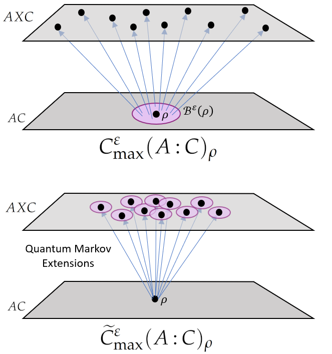
Figure 4: The difference between SMCI and alternative SMCI’s feasible sets visually. For SMCI, $C^{\varepsilon}_{\max}$, the Markov chain extensions of the smoothed state are considered. In contrast, the alternative SMCI, $\widetilde{C}^{\varepsilon}_{\max}$ considers the smoothed state of each Markov chain extension. Note these are effectively the same feasible sets as depicted for two of the formation quantities, $C^{\varepsilon}_{F}$ and $\widetilde{C}^{\varepsilon}_{F}$, in Fig. LABEL:fig:formation-sets.

Hypothesis Testing Common Information

As noted in the introduction, generally an alternative to results in terms of max divergence are results from hypothesis testing divergence. Motivated by this point, we define the hypothesis testing common information.

Definition 10.

Let $\rho_{AC}\in\mathrm{D}(A\otimes C)$. The hypothesis testing common information is given by

$$\widetilde{C}^{\varepsilon}_{h}(A{\,:\,}C)_{\rho}:=\min_{A-X-C}I^{\varepsilon}_{h}(AC{\,:\,}X)_{\rho}\ .$$

The primary point to stress is that unlike with $D_{\max}$, there is no freedom in how we smooth as the smoothing comes from the definition of the measure. As the notation would suggest, this means we can’t, at least directly, use hypothesis testing mutual information to characterize distributed source simulation.

Using that the zero order Petz-Rényi divergence is a limiting case of hypothesis testing divergence (LABEL:eq:hyp-test-div-to-petz), we could view $I^{\varepsilon}_{h}$ as the smoothed version of zero order common information:

$$\widetilde{C}_{0}(A{\,:\,}C)_{\rho}$$

$$:= \min_{A-X-C}D_{0}(\rho_{A-X-C}||\rho_{AC}\otimes\rho_{X})$$

$$= \min_{A-X-C}-\log(\sum_{x:p(x)>0}p(x)\Tr[\Pi_{\rho^{x}_{AC}}\rho_{AC}])\ ,$$

where in the equality we have used (LABEL:eq:hyp-test-div-to-petz). This can be argued to be an intuitive correlation measure in the sense that it intuitively measures how mutually orthogonal the conditional states are, which will be a function of how correlated the $A$ and $C$ spaces are.

Finally, we do note that in contrast to defining correlation measures with $I^{\uparrow\uparrow}_{\max},I^{\downarrow}_{\max}$, we may get cardinality bounds for $\widetilde{C}^{\varepsilon}_{h}$, because it can be written as an expectation over the auxiliary random variable $X$:

$$\exp(-I^{\varepsilon}_{h}(AC{\,:\,}X)_{\rho_{ACX}})=\sum_{x}p(x)D^{\varepsilon}_{h}(\rho^{x}_{AC}||\rho_{AC})\ ,$$

which is an immediate corollary of Proposition 19 in the appendix.

Data-Processing of Common Information Measures

While we won’t need to apply it directly at any point in this work, it is worth noting that (smoothed) common information degrades under local processing, which a correlation measure should. Furthermore, thinking ahead, it tells us that if it takes $\alpha$ amount of randomness to distributed source simulate a target state $\rho_{AC}$ and there are local maps $\Phi,\Psi$ such that $\rho^{\prime}_{A^{\prime}C^{\prime}}=(\Phi\otimes\Psi)(\rho_{AC})$, then it can only require less randomness, i.e.  $\leq\alpha$, to simulate $\rho^{\prime}_{A^{\prime}C^{\prime}}$.

Proposition 5.

For $\varepsilon\in[0,1)$, $C^{\varepsilon}_{\max},\widetilde{C}^{\varepsilon}_{\max},\widetilde{C}^{\varepsilon}_{h}$ are all monotonic under local CPTP maps on both spaces.

Proof.

We begin with $C^{\varepsilon}_{\max}$. We focus on a map being applied on the $A$ space, by symmetry of the argument this will also establish the other case. Let $\widetilde{\rho}_{A-X-C}$ be the minimizer of $C^{\varepsilon}_{\max}(A{\,:\,}C)_{\rho}$. Consider $\Phi(\widetilde{\rho})$ where $\Phi_{A\to A^{\prime}}\in\mathrm{C}(A,A^{\prime})$. Note the resulting state is still a QMC with recovery map $\Phi\circ\mathcal{R}_{X\to AX}$ and $(\Tr_{X}\circ\Phi)(\widetilde{\rho})\in\mathscr{B}^{\varepsilon}(\Phi(\rho))$ by the DPI for purified distance. Then we have,

$$C_{\max}^{\varepsilon}(A^{\prime}{\,:\,}C)_{\Phi(\rho)} \leq I_{\max}(A^{\prime}C{\,:\,}X)_{\Phi(\widetilde{\rho})}$$

$$\leq I_{\max}(AC{\,:\,}B)_{\widetilde{\rho}}=C_{\max}^{\varepsilon}(A{\,:\,}C)_{\rho}\ ,$$

where the first inequality is our choice of element in the smoothed ball and QMC extension and the second is the DPI. Note we needed local maps because we need to preserve the QMC structure.

Similarly, let $(\widehat{\rho}_{A-X-C},\sigma_{AXC})\in\mathrm{QMC}(\rho)\times\mathscr{B}^{\varepsilon}(\widehat{\rho})$ be the optimizers for $\widetilde{C}^{\varepsilon}_{\max}(A{\,:\,}C)_{\rho}$. Then $\Phi(\widehat{\rho})$ is a QMC for the same reason as earlier and $\Phi(\sigma)\in\mathscr{B}^{\varepsilon}(\Phi(\widehat{\rho}))$ by DPI of purified distance. Thus,

$$\widetilde{C}_{\max}^{\varepsilon}(A^{\prime}{\,:\,}C)_{\Phi(\rho)} \leq I_{\max}(A^{\prime}C{\,:\,}X)_{\Phi(\sigma)}$$

$$\leq I_{\max}(AC{\,:\,}B)_{\sigma}=\widetilde{C}_{\max}^{\varepsilon}(A{\,:\,}C)_{\rho}\ ,$$

for the same reasons as before. The same argument holds for $\widetilde{C}^{\varepsilon}_{h}$ as it also satisfies a DPI. ∎

A Remark on Computability

One convenient property of one-shot entropic quantities is that for small dimensions they can be solved easily as they form semidefinite programs [31]. However, here we also have the constraint that we are optimizing over Markov chains. This not only makes it hard to solve in general, but actually means that there must be instances where it is NP-hard to solve, because we can use whether or not the solution is finite as a solution to the separability problem.

Proposition 6.

There exist $\rho_{AC}\in\mathrm{D}(A\otimes C)$ such that computing $C^{\varepsilon}_{\max}(A{\,:\,}C)_{\rho},\widetilde{C}^{\varepsilon}_{\max}(A{\,:\,}C)_{\rho}$ is NP-hard.

Proof.

As established in Proposition 4, $\widetilde{C}^{\varepsilon}_{\max}$ is finite if and only if $\rho_{AC}$ is sufficiently close to the separable state. Likewise for $C^{\varepsilon}_{\max}$ but if it is within some distance from the separable states. Therefore, if it is efficient to compute always, then we have a method for the ability to determine if the state is separable (or within some distance from it). It is known determining membership is strongly NP-hard [43], which means even with some tolerated distance from the set of separable states $\beta$ determining whether it is in or out of the set is NP-hard. Therefore this would be in contradiction with being able to compute $C^{\varepsilon}_{\max},\widetilde{C}^{\varepsilon}_{\max}$ efficiently. ∎

We note the above argument doesn’t say anything about computational complexity when the target distribution is fully classical and thus separable a priori. We also note this is not a problem in terms of establishing our results beyond that it means we cannot in general compute the answer.

V Achievability for Correlation of Formations from One-Shot Soft-Covering Lemma

In effect, Theorem 3 told us when the operational task may be performed at all, i.e. when there is a finite amount of randomness that allows distributed parties to simulate the state (or the same idea for the related tasks). However, it did not tell us how much randomness we will need, which we will show the correlation measures we have introduced will. As mentioned in the introduction, the standard way of establishing the achievable rate for distributed source simulation is a “soft-covering lemma” and in this section we show how to relate a one-shot soft-covering lemma to our correlation measures to establish an achievable rate.

For intuition, we explain the name “soft-covering.” Given the $n-$fold CQ state $\rho_{XB}^{\otimes n}$, by typicality only a fraction of the conditional states $\rho_{B^{\otimes n}}^{x^{n}_{1}}$ are necessary to approximate $\rho_{B}^{\otimes n}$ well. Finding these $x^{n}_{1}$ is non-trivial however, and so a random coding approach is useful. One can draw $M_{n}$ strings $\overline{x}^{n}_{1}\in\mathcal{X}^{\times n}$ according to $p_{X}^{\otimes n}$ to consider an ensemble $\{\rho_{B^{\otimes n}}^{\overline{x^{n}_{1}}}\}$ where each state has probability $|M_{n}|^{-1}$. The soft-covering lemma says that asymptotically if $|M_{n}|\geq I(X{\,:\,}B)_{\rho}$, this ensemble will also approximate $\rho_{B}^{\otimes n}$ with vanishing error. A one-shot soft-covering lemma would then be the same conceptual idea except you draw codewords from $x\in\mathcal{X}$ rather than $x^{n}_{1}\in\mathcal{X}^{\times n}$, and so the correlation measure presumably would need to be larger than mutual information.

Recently, a one-shot soft-covering lemma for quantum states that is optimal to second-order was established [26]. The authors do this by establishing achievability in terms of a mutual-information-like information spectrum divergence quantity and then converting to the hypothesis testing mutual information as defined in (LABEL:eq:hyp-mut-inf-def). As remarked upon in the correlation measure section, we do not expect to capture distributed source simulation from the hypothesis testing divergence. However, as noted in Section III, it is equally valid to convert to smooth max divergence from the information spectrum divergence [33], and we suspect the authors of [26] omitted this as their converse proof is less natural to convert to smooth max mutual information. As our interest is in a task whose converse is ultimately characterized in terms of a max mutual information induced measure, we will explain how to obtain the smooth max mutual information version of the result from [26] as well as present the hypothesis testing result. To state this, we need three preliminaries: the definition of ‘minimal random codebook size for $\varepsilon-$covering’ from [26] except we will need to alter it up to a factor of a half. We will also need to establish a few mutual information measures that will allows us to express all bounds in a notationally similar fashion.

Definition 11.

([26] Altered) Let $\rho_{XB}=\sum_{x\in\mathcal{X}}p(x)\outerproduct{x}{x}\otimes\rho_{B}^{x}$. The minimal random codebook size for $\varepsilon-$covering, denoted by $M^{\varepsilon}(B{\,:\,}X)_{\rho}$ is given by

$$\inf_{M\in\mathbb{N}}\Bigg{\{}|\mathcal{C}|\leq M\,\&\,\mathbb{E}_{\mathcal{C}\sim p_{X}}\left\|\frac{1}{|\mathcal{C}|}\sum_{x\in\mathcal{C}}\rho^{x}_{B}-\rho_{B}\right\|_{1}\leq\varepsilon\Bigg{\}}\ .$$

Note that taking the logarithm of $M^{\varepsilon}(B{\,:\,}X)_{\rho}$ is the number of bits needed to describe an element of the random code.

Proposition 7.

For $\rho\in\mathrm{D}_{\leq}(A\otimes B)$, the following two properties hold:

1. $I^{\varepsilon}_{h}(A{\,:\,}B)_{\rho}=I^{\varepsilon}_{h}(B{\,:\,}A)_{\rho}$.

2. $D^{\varepsilon}_{s}(\rho_{AB}||\rho_{A}\otimes\rho_{B})=D^{\varepsilon}_{s}(\rho_{BA}||\rho_{B}\otimes\rho_{A})$.

Proof.

1) $Q$ is feasible for $D^{\varepsilon}_{h}(\rho_{AB}||\rho_{A}\otimes\rho_{B})$ if and only if $\mathrm{SWAP}_{A\leftrightarrow B}(Q)$ is feasible for $D^{\varepsilon}_{h}(\rho_{BA}||\rho_{B}\otimes\rho_{A})$, where $\mathrm{SWAP}_{A\leftrightarrow B}$ is the CPTP map that re-orders the spaces. This is because

$$\Tr[Q\rho_{A}\otimes\rho_{B}]$$ (15)

$$= \Tr[\mathrm{SWAP}_{A\leftrightarrow B}(Q)\mathrm{SWAP}_{A\leftrightarrow B}(\rho_{A}\otimes\rho_{B})]$$

$$= \Tr[\mathrm{SWAP}_{A\leftrightarrow B}(Q)\rho_{B}\otimes\rho_{A}]\ ,$$

and the same argument for $\rho_{AB}$. As swapping the ordering of the spaces preserves positivity, we have the feasible set for $I^{\varepsilon}_{h}(B{\,:\,}A)_{\rho}$ is the same as $I^{\varepsilon}_{h}(A{\,:\,}B)_{\rho}$ up to a swapping of spaces and moreover (LABEL:eq:flip-hyp-mut-inf) tells us the objective function values are the same. This completes the proof of the first claim.

2) Recall from (7) that $D^{\varepsilon}_{s}(\rho_{AB}||\rho_{A}\otimes\rho_{B})=\sup\{R\in\mathbb{R}|\Tr[\rho_{AB}\{\rho_{AB}\leq 2^{R}\rho_{A}\otimes\rho_{B}\}]\leq\varepsilon\}$. Note for any $R$, $\{\rho_{AB}\leq 2^{R}\rho_{A}\otimes\rho_{B}\}\equiv\Pi$ is the projector onto the non-negative eigenspace of $2^{R}\rho_{A}\otimes\rho_{B}-\rho_{AB}$. It follows $\mathrm{SWAP}_{A\leftrightarrow B}(\Pi)$ is the projector onto the non-negative eigenspace of $2^{R}\rho_{B}\otimes\rho_{A}-\rho_{BA}$. Thus, for all $R\in\mathbb{R}$,

$$\Tr[\rho_{AB}\{\rho_{AB}\leq 2^{R}\rho_{A}\otimes\rho_{B}\}]$$

$$= \Tr[\rho_{BA}\{\rho_{BA}\leq 2^{R}\rho_{B}\otimes\rho_{A}\}]\ .$$

This implies the claim as the feasible $R$ for fixed $\varepsilon$ is the same for both. ∎

With these addressed, we state the one-shot soft-covering lemma and provide the part not proven in the cited paper.

Lemma 8.

([26, Theorem 13 Achievability + A Little More]) Let $\rho_{XB}\in\mathrm{D}(X\otimes B)$ and $\varepsilon\in(0,1)$. If $\delta\in(0,\varepsilon)$ and $\eta\in(\frac{7}{8}\varepsilon,\varepsilon)$, then

$$\log(M^{\varepsilon}(B{\,:\,}X)_{\rho})$$ (16)

$$\hskip 8.5359pt\leq I^{\uparrow,\sqrt{\varepsilon-\eta}}_{\max}(B{\,:\,}X)_{\rho}+\log(\nu)+g(\overline{\varepsilon})+$$

$$\hskip 28.45274pt-\log(1/\varepsilon-1/8)+3\log 3+7\ ,$$

where $\nu\equiv|\mathrm{\mathrm{spec}}(\rho_{B})|$, the number of distinct eigenvalues of $\rho_{B}$, $\overline{\varepsilon}=2+\widetilde{\varepsilon}-2\sqrt{1-\widetilde{\varepsilon}}$, and $\widetilde{\varepsilon}=\sqrt{\varepsilon/8}-\sqrt{\varepsilon-\eta}>0$.
Similarly,

$$\log(M^{\varepsilon}(B{\,:\,}X)_{\rho})$$ (17)

$$\hskip 14.22636pt\leq I^{1-\varepsilon/8}_{h}(B{\,:\,}X)_{\rho}+\log(\nu\cdot\nu^{\prime})-2\ ,$$

where $\nu^{\prime}=|\mathrm{spec}(\rho_{X}\otimes\rho_{B})|$.

Remark 2.

We note our spectral terms for hypothesis testing mutual information differ from [26]. Our scaling is made explicit in the proof.

Proof.

The proof for $I^{\varepsilon}_{h}$ is effectively found in [26] except that we changed the factor of half of which one has to keep track. How to address that is shown equivalently in proving the bound in terms of $I^{\uparrow\uparrow,\varepsilon}_{\max}$, so we don’t show it explicitly. To establish the bound in terms of $I^{\uparrow\uparrow,\varepsilon}_{\max}$, the proof is still primarily found in [26], we just start from [26, Equation 4.2] where we multiply both sides by 2:

$$\mathbb{E}_{\mathcal{C}}\left\|\frac{1}{|\mathcal{C}|}\sum_{x\in\mathcal{C}}\rho^{x}_{B}-\rho_{B}\right\|_{1}$$ (18)

$$\hskip 14.22636pt\leq 2\Tr[\rho_{XB}\{\mathbb{P}_{\rho_{B}}(\rho_{XB})>c\rho_{X}\otimes\rho_{B}\}]$$

$$\hskip 85.35826pt+2\sqrt{\frac{|\mathrm{spec}(\rho_{B})|c}{|\mathcal{C}|}}\ ,$$

where $\mathbb{P}_{\rho_{B}}$ is the pinching map on $B$ according to $\rho_{B}$ and $c>0$. Then let $\delta\in(0,\varepsilon)$ and choose

$$c\equiv\exp{D_{s}^{1-(\varepsilon-\delta)/2}(\mathbb{P}_{\rho_{B}}(\rho_{XB})||\rho_{X}\otimes\rho_{B})+\zeta\}}$$

for some small $\zeta>0$. The reason to define $c$ in this manner is because, by definition of $\varepsilon-$information spectrum divergence (7) we obtain:

$$\Tr[\rho_{XB}\{\mathbb{P}_{\rho_{B}}(\rho_{XB})>c\rho_{X}\otimes\rho_{B}\}]$$

$$= \Tr[\mathbb{P}_{\rho_{B}}(\rho_{XB})\{\mathbb{P}_{\rho_{B}}(\rho_{XB})>c\rho_{X}\otimes\rho_{B}\}]$$

$$= 1-\Tr[\mathbb{P}_{\rho_{B}}(\rho_{XB})\{\mathbb{P}_{\rho_{B}}(\rho_{XB})\leq c\rho_{X}\otimes\rho_{B}\}]$$

$$< 1-(1-(\varepsilon-\delta)/2)$$

$$= (\varepsilon-\delta)/2$$

where the first equality is because the projected space doesn’t change, and the strict inequality is using our definition of $c$ with the definition of $\varepsilon-$information spectrum along with including small $\zeta$ and . Letting $|\mathcal{C}|=\lceil|\mathrm{spec}(\rho_{B})|c(2/\delta)^{-2}\rceil$ and plugging these bounds into (18) gets the target $\mathbb{E}_{\mathcal{C}}\left\|\frac{1}{|\mathcal{C}|}\sum_{x\in\mathcal{C}}\rho^{x}_{B}-\rho_{B}\right\|_{1}\leq\varepsilon$.

We remark so far the only change from the original proof is that we scaled $\varepsilon,\delta$ by two. To now establish bounds in terms of max mutual information, we will pick $\varepsilon\in(0,1/2)$ as explained at the start of the proof and we will let $\delta=\varepsilon/2$. We define $\varepsilon^{\prime}\equiv 1-\varepsilon/8$, $\delta^{\prime}\equiv\varepsilon/8$. By our choice of $|\mathcal{C}|$,

$$\log(M^{\varepsilon}(B{\,:\,}X)_{\rho})$$

$$\leq\log|\mathcal{C}|$$

$$\leq D_{s}^{1-(\varepsilon-\delta)/2}(\mathbb{P}_{\rho_{B}}(\rho_{XB})||\rho_{X}\otimes\rho_{B})+\zeta$$

$$\hskip 71.13188pt+\log|\mathrm{spec}(\rho_{B})|+2\log(\delta)$$

$$=D_{s}^{1-(\varepsilon-\delta)/2}(\mathbb{P}_{\rho_{B}}(\rho_{BX})||\rho_{B}\otimes\rho_{X})+\zeta$$

$$\hskip 71.13188pt+\log(\nu)+2\log(\delta)$$

$$=D_{s}^{\varepsilon^{\prime}-\delta^{\prime}}(\mathbb{P}_{\rho_{B}}(\rho_{BX})||\rho_{B}\otimes\rho_{X})+\zeta$$

$$\hskip 71.13188pt+\log(\nu)+2\log(\delta)$$

$$\leq D^{\sqrt{1-\varepsilon^{\prime}}}_{\max}(\rho_{BX}||\rho_{B}\otimes\rho_{X})+\log(\nu)$$

$$\hskip 71.13188pt+2\log(\delta)-3\log(\delta^{\prime})+\log(\varepsilon^{\prime})$$

$$\hskip 78.24507pt+3\log(3)+\zeta$$

$$=I^{\uparrow\uparrow,\sqrt{\varepsilon/8}}_{\max}(B{\,:\,}X)_{\rho}+\log(\nu)-\log(1/\varepsilon-1/8)$$

$$\hskip 64.01869pt+3\log 3+7+\zeta\ ,$$

where the first inequality is by definition, the second is our definition of $|\mathcal{C}|$, the first equality is by Item 2 of Proposition 7, the second equality is our definitions as $1-\varepsilon/2+\varepsilon/4=1-\varepsilon/4=\varepsilon^{\prime}-\delta^{\prime}$, the third inequality is [33, Eqn. 17] and where we have used $\mathbb{P}_{\rho_{B}}(\rho_{XB})=\mathbb{P}_{\rho_{X}\otimes\rho_{B}}(\rho_{XB})$ as $\rho_{XB}$ is classical on the $X$ register, the fifth is by definition and merging the logarithm terms. As $\zeta>0$ was arbitrary, we let $\zeta$ tend to zero so that it goes away.

Lastly, we wish to upper bound $I^{\uparrow\uparrow,\sqrt{\varepsilon/8}}_{\max}$ by $I^{\uparrow,\sqrt{\varepsilon-\eta}}_{\max}$ by applying Lemma 1. This means we need $\sqrt{\varepsilon-\eta}<\sqrt{\varepsilon/8}$, so $\eta\in(\frac{7}{8},1)\cdot\varepsilon$. Then we need to solve $0<\widetilde{\varepsilon}:=\sqrt{\varepsilon/8}-\sqrt{\varepsilon-\eta}=\overline{\varepsilon}+2\sqrt{\overline{\varepsilon}}$ for $\overline{\varepsilon}$. The equation $a=x+2\sqrt{x}$ holds for $x=2+a-\sqrt{1+a}$. Thus, $\overline{\varepsilon}=2+\widetilde{\varepsilon}-2\sqrt{1+\widetilde{\varepsilon}}$. Plugging this value into Lemma 1 gets the max mutual information bound.

To get the hypothesis testing bound, it is effectively the same as in [26]. One starts from the second equality in the chain of inequalities above except $\varepsilon^{\prime}\equiv 1-\frac{3\varepsilon}{16}$ and $\delta^{\prime}\equiv\varepsilon/16$. Now we will bound the spectrum divergence term where we again use $\mathbb{P}_{\rho_{B}}(\rho_{BX})=\mathbb{P}_{\rho_{B}\otimes\rho_{X}}(\rho_{BX})$,

$$D^{\varepsilon^{\prime}-\delta^{\prime}}_{s}(\mathbb{P}_{\rho_{B}\otimes\rho_{X}}(\rho_{BX})||\rho_{B}\otimes\rho_{X})$$

$$\leq D^{\varepsilon^{\prime}}_{s}(P||Q)-\log(\delta^{\prime})$$

$$= D^{\varepsilon^{\prime}+\delta^{\prime}-\delta^{\prime}}_{s}(P||Q)-\log(\delta^{\prime})$$

$$\leq D^{\varepsilon^{\prime}+\delta^{\prime}}_{h}(\rho_{XB}||\rho_{X}\otimes\rho_{B})+\log(\nu^{\prime})-2\log(\delta^{\prime})$$

$$= I_{h}^{1-\varepsilon/8}(B:X)_{\rho}+\log(\nu^{\prime}/\varepsilon^{2})+8\ ,$$

where the first inequality is [33, Eqn. 19] and $P,Q$ are the Nussbaum-Szkoła distributions as discussed in [33] and the second inequality is [33, Eqn. 28] as the inequality always holds for $\theta(\sigma)$ replaced with $\nu^{\prime}$. The equalities just use definitions of $\varepsilon^{\prime},\delta^{\prime}$. We combine this with the bound we started from and this completes the proof. ∎

We are now ready to prove achievability of distributed source simulation for quantum states from the above one-shot soft covering lemma. The idea is that if the state $\rho_{AC}$ can be sufficiently approximated by a separable state $\widetilde{\rho}_{AC}$, then there is a QMC extension $\widetilde{\rho}_{A-X-C}$ with recovery maps $\mathcal{R},\overline{\mathcal{R}}$ which will allow us to source simulate using the random codebook rate. Note in particular this means that for separable states, one can source simulate to arbitrary non-zero error, but for an entangled state, there is a fundamental limit.

Lemma 9.

Let $\varepsilon\in(0,1)$. Let $\rho_{AC}\in\mathrm{D}(A\otimes C)$ such that $2E_{T}(A:C)_{\rho}\neq\varepsilon$. Let $\varepsilon_{1},\varepsilon_{2}\in(0,1)$ such that $2\varepsilon_{1}+\varepsilon_{2}<\varepsilon$. Then,

$$C^{\varepsilon}_{U,F}(A{\,:\,}C)_{\rho} \leq C^{\varepsilon_{1}}_{\max}(A{\,:\,}C)_{\rho}+\kappa(\varepsilon_{2})\ ,$$

where the $\kappa(x):=\log(\nu)+g(\overline{x})-\log(1/x-1/8)+3\log 3+7$. Moreover, there exist choices of $\varepsilon_{1},\varepsilon_{2}$ such that this is finite whenever $2E_{T}(A{\,:\,}C)_{\rho}<\varepsilon$, so it holds for all separable states.

Furthermore, if $\rho_{AC}\in\mathrm{Sep}\mathrm{D}(A{\,:\,}C)$, and $\eta\in(7/8\varepsilon,\varepsilon)$,

$$\{\widetilde{C}^{\varepsilon}_{F}(A{\,:\,}C)_{\rho},\widehat{C}^{\varepsilon}_{F}(A{\,:\,}C)_{\rho}\}$$

$$\leq \min\{\widetilde{C}^{\sqrt{\varepsilon-\eta}}_{\max}(A{\,:\,}C)_{\rho}+\kappa(\varepsilon),$$

$$\hskip 28.45274pt\widetilde{C}^{1-\varepsilon/8}_{h}(A{\,:\,}C)_{\rho}+\log(\nu\cdot\nu^{\prime})-2\}\ .$$

Proof.

Define $2E_{T}(A{\,:\,}C)_{\rho}=\delta_{E}<\varepsilon$. Let $\varepsilon_{1}\in(\delta_{E}/2,\varepsilon/2)$. Let $\varepsilon_{2}\in(0,\varepsilon-2\varepsilon_{1})$. By our choice of $\varepsilon_{1}$, it follows that there is at least one separable state contained in $\mathscr{B}^{\varepsilon_{1}}(\rho)$. Denote an arbitrary choice $\widetilde{\rho}_{AC}$. By Lemma 2, we can think of $\widetilde{\rho}_{AC}$ as the marginal of the CQ state $\rho_{A-X-C}=\sum_{x\in\mathcal{X}}p(x)\outerproduct{x}{x}\otimes\rho_{x}^{A}\otimes\rho_{x}^{C}$. By definition, $M^{\varepsilon_{2}}(AC{\,:\,}X)_{\widetilde{\rho}_{A-X-C}}$ is the minimal size such that the expectation over random codebooks is a $\varepsilon-$covering. It follows for this size of codebook, there must exist a a codebook $\mathcal{C}^{\prime}$ with size $M^{\varepsilon_{2}}(AC{\,:\,}X)_{\rho}$ that is a $\varepsilon_{2}-$covering. Fix this codebook $\mathcal{C}^{\prime}$ and let $|\widehat{X}|:=M^{\varepsilon_{2}}(AC{\,:\,}X)_{\widetilde{\rho}}$. Note that using the Markov chain extension, we have that the ensemble is of the form $\{\widetilde{\rho}^{A}_{x}\otimes\widetilde{\rho}^{C}_{x}\}_{x\in\mathcal{C}^{\prime}}$ with each element equiprobable and by Lemma 8 it satisfies $\|\frac{1}{|\mathcal{C}^{\prime}|}\sum_{x\in\mathcal{C}^{\prime}}\widetilde{\rho}_{x}^{A}\otimes\widetilde{\rho}_{x}^{C}-\widetilde{\rho}_{AC}\|_{1}\leq\varepsilon_{2}\ .$ Using our definition of $\varepsilon_{1},\varepsilon_{2}$ along with the fact that (4) tells us purified distance upper bounds trace distance, we have

$$\left\|\frac{1}{|\mathcal{C}^{\prime}|}\sum_{x\in\mathcal{C}^{\prime}}\widetilde{\rho}_{x}^{A}\otimes\widetilde{\rho}_{x}^{C}-\rho_{AC}\right\|_{1}\leq 2\varepsilon_{1}+\varepsilon_{2}<\varepsilon\ .$$ (19)

We will now build the strategy using this. Let the distributed source produce $\chi^{|\pi}_{\widehat{X}\widehat{X}^{\prime}}$ and distribute the $\widehat{X}$ register to Alice and $\widehat{X}^{\prime}$ to Bob. Now note that the recovery maps’ actions are of the form $\mathcal{R}:\outerproduct{x}{x}\mapsto\widetilde{\rho}^{x}_{C}\otimes\outerproduct{x}{x}$, $\overline{\mathcal{R}}:\outerproduct{x}{x}\mapsto\widetilde{\rho}^{x}_{A}\otimes\outerproduct{x}{x}$. Therefore, upon receiving their copies of $\outerproduct{x}{x}$, they may apply their recovery maps. Ignoring their local copies of $\outerproduct{x}{x}$, the joint state is then

$$\frac{1}{|\mathcal{C}^{\prime}|}\sum_{x\in\mathcal{C}^{\prime}}\widetilde{\rho}^{A}_{x}\otimes\widetilde{\rho}^{C}_{x}\ .$$

It follows from (19) that this generated state is a distributed source simulation to error $\varepsilon$ and thus $\log(M^{\varepsilon_{2}}(AC{\,:\,}X)_{\widetilde{\rho}_{A-X-C}})=H_{0}(\widehat{X})_{\chi}$ is an upper bound on $C^{\varepsilon}_{U,F}(A{\,:\,}C)_{\rho}$. As the choice of Markov chain extension we picked was arbitrary, we can infimize over the choices. However, as we established in Lemma 7, the dimension of $X$ may be bounded, and so this becomes a minimization. Moreover, we could minimize over a $\mathscr{B}^{\varepsilon_{1}}(\rho)$ as every state $\sigma$ contained satisfies $\|\sigma-\rho\|_{1}\leq 2\varepsilon_{1}$. Therefore, we have

$$C^{\varepsilon}_{U,F}(A{\,:\,}C)_{\rho}\leq \min_{\widetilde{\rho}\in\mathscr{B}^{\varepsilon_{1}}(\rho)}\min_{A-X-C}I^{\sqrt{\varepsilon_{2}-\eta}}_{\max}(AC{\,:\,}X)_{\widetilde{\rho}}+\kappa$$

$$= \min_{\widetilde{\rho}\in\mathscr{B}^{\varepsilon_{1}}(\rho)}\widetilde{C}^{\varepsilon_{2}-\eta}_{\max}(A{\,:\,}C)_{\widetilde{\rho}}+\kappa(\varepsilon_{2})\ ,$$

where we used Lemma 8. To get the second upper bound in the lemma, we note the following. First, $C_{\max}(A{\,:\,}C)=\widetilde{C}^{0}_{\max}(A{\,:\,}C)$. Second, $\widetilde{C}^{\varepsilon}_{\max}$ monotonically decreases as smoothing parameter $\varepsilon$ increases. Therefore,

$$C^{\varepsilon_{1}}_{\max}(A{\,:\,}C)_{\rho}= \min_{\widetilde{\rho}\in\mathscr{B}^{\varepsilon_{1}}(\rho)}\widetilde{C}^{0}_{\max}(A{\,:\,}C)_{\widetilde{\rho}}$$

$$\geq \min_{\widetilde{\rho}\in\mathscr{B}^{\varepsilon_{1}}(\rho)}\widetilde{C}^{\sqrt{\varepsilon_{2}-\eta}}_{\max}(A{\,:\,}C)_{\widetilde{\rho}}\ ,$$

which establishes this second upper bound.

For the moreover statements, note we could do the same argument on Markov chain extensions of $\rho_{AC}$ so long as $\rho_{AC}$ is separable by Lemma 2, and then we only have a single smoothing parameter. ∎

VI Converses for Correlation of Formations

With the achievability established from the one-shot cover lemma, we stress why the one-shot converse for random coding is insufficient. The converse for the minimal random codebook size for $\varepsilon-$covering gets the minimal size to achieve an $\varepsilon-$covering with respect to expectation over random codebooks. What we are interested in is the minimal size for any codebook to achieve distributed source simulation. As these are distinct settings, we turn our attention to establishing a converse to the one relevant for our purposes. This will follow from the DPI of the measures that induce the common informations and the relationship between $C_{\max}$ and $H_{0}$ for perfectly correlated classical states $\chi$, which we now establish.

Proposition 8.

For any distribution $p\in\mathcal{P}(\mathcal{X})$, let $\chi^{|p}_{XX^{\prime}}=\sum_{x}p(x)\outerproduct{x}{x}\otimes\outerproduct{x}{x}$. Then $C_{\max}(X{\,:\,}X^{\prime})_{\chi}=H_{0}(X)_{\chi}$.

Proof.

First note that the optimal Markov chain is $p_{XX^{\prime}\widetilde{X}}=\sum_{x}p(x)\outerproduct{x}{x}^{\otimes 3}$ whose recovery maps are merely copying. While intuitive, one also may make this rigorous in the following manner. The seed will have to be $\sum_{y}p^{\prime}(y)$. By symmetry, the recovery maps for both parties will be conditional distributions $\{q(x|y)\}_{y\in\mathcal{Y}}$. These conditional distributions will in fact have to be deterministic as otherwise the $X$ and $X^{\prime}$ spaces won’t be perfectly correlated. Thus $\sum_{y}p^{\prime}(y)$ can be partitioned into sets $\mathcal{Y}_{x_{i}}:=\{y\in\mathcal{Y}:q(x_{i}|y)=1\}$ and then we can apply a coarse graining map that takes $\Phi$ that takes $\mathcal{Y}_{x_{i}}\to x_{i}$ for all $i$. Note $\Phi(p_{XX^{\prime}Y})=p_{XX^{\prime}\widetilde{X}}$ and as it is a coarse graining map, by data-processing, $I_{\max}(XX^{\prime}{\,:\,}\widetilde{X})_{p_{XX^{\prime}\widetilde{X}}}=I_{\max}(XX^{\prime}{\,:\,}\widetilde{X})_{\Phi(p_{XX^{\prime}Y})}\leq I_{\max}(XX^{\prime}{\,:\,}Y)_{p_{XX^{\prime}Y}}$. Thus, as we want to minimize $I_{\max}$, this establishes we have the optimal Markov chain.

With this established, by Corollary 2, we have

$$I_{\max}(XX^{\prime}{\,:\,}\widetilde{X})_{p_{XX^{\prime}\widetilde{X}}}$$ (20)

$$\hskip 14.22636pt=\log(\sum_{x}p(x)\exp(I_{\max}(p^{x}_{XX^{\prime}}||p_{X})))\ .$$

Noting $p^{x}_{XX^{\prime}}=\outerproduct{x}{x}^{\otimes 2}$,

$$I_{\max}(p^{x}_{XX^{\prime}}||p_{X})$$

$$= \min_{q\in\mathcal{P}(\mathcal{X}^{\prime})}\Bigg{\{}\lambda:\outerproduct{x}{x}^{\otimes 2}\leq 2^{\lambda}p_{X}\otimes\sum_{x^{\prime\prime}}q(x^{\prime\prime})\outerproduct{x^{\prime}}{x^{\prime}}\Bigg{\}}$$

$$= \min\left\{\lambda:\outerproduct{x}{x}^{\otimes 2}\leq 2^{\lambda}p(x^{\prime})\outerproduct{x^{\prime}}{x^{\prime}}\otimes\outerproduct{x}{x}\,\forall x^{\prime}\right\}$$

$$= \min\left\{\lambda:1\leq 2^{\lambda}p(x)\right\}\Rightarrow\lambda=p(x)^{-1}\ ,$$

where in the first line we have just used the definition and Proposition 15, in the second we have used it is clear that $q_{X}=\outerproduct{x}{x}$ will decrease $\lambda$ and then we are dealing with diagonal operators so the bound must hold entry-wise, the third is because the L.H.S. only has support on $\outerproduct{x}{x}^{\otimes 2}$ and this completes the argument. Therefore, plugging this into (20), we

$$I_{\max}(XX^{\prime}{\,:\,}\widetilde{X})_{p_{XX^{\prime}\widetilde{X}}}$$

$$= \log(\sum_{x}p(x)\exp(\log(1/p(x))))$$

$$= \log(\sum_{x}1)=\log(|\mathcal{X}|)=H_{\max}(X)_{\chi}\ .$$

This completes the proof. ∎

We now present the one-shot converses. We note the square root in the correlation measure is due to purified distance smoothing rather than something fundamental per se. We begin with establishing the converse for correlation of formation, i.e. distributed source simulation. We again stress that the results hold for the entire range of smoothing parameters so long as the state is separable.

Lemma 10.

Let $\varepsilon\in(0,1)$. Let $\rho_{AC}\in\mathrm{D}(A\otimes C)$ such that $2E_{T}(\rho)<\varepsilon$.

$$C^{\sqrt{\varepsilon}}_{\max}(A{\,:\,}C)_{\rho}\leq C^{\varepsilon}_{F}(A{\,:\,}C)_{\rho}\leq C^{\varepsilon}_{U,F}(A{\,:\,}C)_{\rho}\ .$$

In particular, the bound holds for any $\rho_{AC}\in\mathrm{Sep}\mathrm{D}(A{\,:\,}C)$.

Proof.

Let $C^{\varepsilon}_{F}(A{\,:\,}C)_{\rho}=n<\infty$ where $n$ is finite because $E_{T}(\rho)<\varepsilon$ so there is $\widehat{\rho}_{AC}\in\mathrm{Sep}(A{\,:\,}C)$ such that $\widehat{\rho}_{AC}\approx_{\varepsilon}^{\mathrm{TD}}\rho_{AC}$. This means, $P(\widehat{\rho}_{AC},\rho)\leq\sqrt{\varepsilon}$. Moreover, by Lemmas 2 and 2, this means there exists $\widehat{\rho}_{A-\widetilde{X}-C}$ such that $\|\widehat{\rho}_{AC}-\rho_{AC}\|_{1}\leq\varepsilon$ and $|\widetilde{X}|=n$ is finite. Define $\mathcal{X}^{|p}$ with respect to the distribution defining $\rho_{X}$. The recovery maps are preparation channels so that $\mathcal{R}_{\widetilde{X}\to\widetilde{X}A}$ Define $\mathcal{R}_{\widetilde{X}\to A}\equiv\Tr_{X}\circ\mathcal{R}$ and likewise for $\overline{\mathcal{R}}$. It follows $\widehat{\rho}_{A-\widetilde{X}-C}=(\overline{\mathcal{R}}_{\widetilde{X^{\prime}}\to C}\circ\mathcal{R}_{\widetilde{X}\to A})(\chi^{|p}_{X\widetilde{X}X^{\prime}})$. Then we have

$$C^{\sqrt{\varepsilon}}_{\max}(A{\,:\,}C)_{\rho}$$

$$= \min_{\widetilde{\rho}\in\mathscr{B}^{\sqrt{\varepsilon}}(\rho)}\min_{\widetilde{\rho}_{A-\widetilde{X}-C}}I_{\max}(AC{\,:\,}\widetilde{X})_{\widetilde{\rho}}$$

$$\leq I_{\max}(AC{\,:\,}\widetilde{X})_{\widehat{\rho}}$$

$$= I_{\max}(AC{\,:\,}\widetilde{X})_{(\overline{\mathcal{R}}\circ\mathcal{R})(\chi)}$$

$$\leq I_{\max}(XX^{\prime}{\,:\,}\widetilde{X})_{\chi}=H_{0}(X)_{\chi}=n=C^{\varepsilon}_{F}(A{\,:\,}C)_{\rho}\ ,$$

where the first equality is by definition, the first inequality is by our choice of $\widehat{\rho}$ being feasible, the second equality is by the equivalence established previously, the second inequality is by data processing, and the last steps are by Proposition 8 and our assumption respectively. This completes the proof. ∎

We now present the converse for the entanglement-assisted correlation of formation and the private correlation of formation.

Lemma 11.

Let $\rho_{AC}\in\mathrm{Sep}\mathrm{D}(A{\,:\,}C)$. Then

$$\widetilde{C}^{\sqrt{\varepsilon}}_{\max}(A{\,:\,}C)\leq\widetilde{C}^{\varepsilon}_{F}(A{\,:\,}C)\leq\widehat{C}^{\varepsilon}_{F}(A{\,:\,}C)\ .$$

Moreover, for $\delta\in(0,1-\varepsilon)$,

$$\widetilde{C}_{h}^{1-\varepsilon-\delta}(A{\,:\,}C)+3\log(\delta)-3\log 3-\log(1-\varepsilon)$$

$$\hskip 85.35826pt\leq\widetilde{C}^{\varepsilon}_{F}(A{\,:\,}C)\leq\widehat{C}^{\varepsilon}_{F}(A{\,:\,}C)\ .$$

Proof.

As $\widetilde{C}^{\varepsilon}_{F}\leq\widehat{C}^{\varepsilon}_{F}$, one can focus on $\widetilde{C}^{\varepsilon}_{F}$. The proof for $\widetilde{C}^{\varepsilon}_{F}$ is effectively the same as the previous except we need $\rho_{A-X-C}\in\mathrm{Sep}\mathrm{D}(A{\,:\,}C)$ for the value to be finite and then we consider a preparation channels of the form $\Phi:x\mapsto\sigma_{AC}^{x}$ where $\|\sigma_{A\widetilde{X}C}-\rho_{A-\widetilde{X}-C}\|_{1}\leq\varepsilon$ and $|\widetilde{X}|=n$, but as we consider DPI for $I_{\max}$ this does not conflict with Proposition 5. Finally, to get the hypothesis testing bound, one defines $\sqrt{1-\overline{\varepsilon}}=\varepsilon$ and applies [33, Eqn. 22]. ∎

Finally, we may combine the results into our one-shot bound for distributed source simulation and its entanglement-assisted equivalent. These were reported in the summary of results, but for simplicity we re-state them here with proof.

Theorem 12.

Let $\varepsilon\in(0,1)$. Let $\rho_{AC}\in\mathrm{D}(A\otimes C)$ with $2E_{T}(A{\,:\,}C)_{\rho}<\varepsilon$. Let $\varepsilon_{1},\varepsilon_{2}\in(0,1)$ such that $2\varepsilon_{1}+\varepsilon_{2}<\varepsilon$. Then,

$$C^{\sqrt{\varepsilon}}_{\max}(A{\,:\,}C)_{\rho} \leq C^{\varepsilon}_{F}$$

$$\leq C^{\varepsilon}_{U,F}\leq C^{\varepsilon_{1}}_{\max}(A{\,:\,}C)_{\rho}+\kappa\ ,$$

where $\kappa$ is defined in Lemma 9.

Proof.

As $2E_{T}(A:C)_{\rho}<\varepsilon$ was the constraint in both Lemmas 9 and 10, we’ve satisfied the conditions to apply them both. ∎

Theorem 13.

Let $\rho_{AC}\in\mathrm{Sep}\mathrm{D}(A{\,:\,}C)$. If $\delta\in(0,\varepsilon)$ and $\eta\in(\frac{7}{8}\varepsilon,\varepsilon)$, then

$$\widetilde{C}^{\sqrt{\varepsilon}}_{\max}(A{\,:\,}C)_{\rho}\leq \{\widetilde{C}^{\varepsilon}_{F}(A{\,:\,}C)_{\rho},\widehat{C}^{\varepsilon}_{F}(A{\,:\,}C)_{\rho}\}$$

$$\leq \widetilde{C}^{\sqrt{\varepsilon-\eta}}_{\max}(A{\,:\,}C)_{\rho}+\kappa\ ,$$

or if $\delta^{\prime}\in(0,1-\varepsilon)$,

$$\widetilde{C}_{h}^{1-\varepsilon-\delta^{\prime}}(A{\,:\,}C)_{\rho}+\gamma$$

$$\hskip 28.45274pt\leq\{\widetilde{C}^{\varepsilon}_{F}(A{\,:\,}C)_{\rho},\widehat{C}^{\varepsilon}_{F}(A{\,:\,}C)_{\rho}\}$$

$$\hskip 56.9055pt\leq\widetilde{C}^{1-\varepsilon/8}_{h}(A{\,:\,}C)_{\rho}+\log(\nu\cdot\nu^{\prime})-2\ ,$$

where $\gamma\equiv 3\log(\delta^{\prime})-3\log 3-\log(1-\varepsilon)$.

Proof.

The conditions stated mean we satisfy the conditions of Lemmas 9 and Lemma 11 at the same time. ∎

VII Recovering Asymptotic Results via a Weak AEP

Theorems 12 and 13 provide one-shot rates of distributed source simulation and its entanglement-assisted counterpart. A natural, and perhaps necessary, question would be whether we can in fact recover Wyner’s asymptotic result, and Hayashi’s extension, from our one-shot bounds. There are a few reasons for this question being so important. First, while we have established one-shot achievable and converse bounds, it is not a priori obvious these bounds will asymptotically converge properly, though it would be surprising if they did not given previous work on the smooth entropy framework. Second, we have actually established bounds for an operational task more general than Wyner’s setting. That is, we have established upper and lower bounds for distributed source simulation where the randomness is not uniform, i.e. $C^{\varepsilon}_{F}$, as well as when it is uniform, $C^{\varepsilon}_{U,F}$. It would therefore be interesting to determine whether this setting has the same asymptotic rate. Finally, as was discussed in determining the correlation measures themselves, there seem to be further nuances in how these correlation measures work. Indeed, as noted in the introduction, $I^{\uparrow,\varepsilon}_{\max}$ inherits a strong AEP from its chain rule decomposition into smooth min- and max-entropies and their AEPs. However, for this to hold, every register must be $n-$fold, but as we optimize over an extension, we lose this structure. Therefore, any asymptotic behaviour we can prove is new. In this section we establish weak AEPs for our max mutual information induced correlation measures, as we summarize in the following theorem.

Definition 12.

For $\rho_{AC}\in\mathrm{D}(A\otimes C)$, the Wyner Common information is defined as

$$C(A{\,:\,}C)_{\rho}:=\min_{A-X-C}I(AC{\,:\,}X)\ ,$$

where the minimization is over QMC extensions of $\rho_{AC}$.

Theorem 14.

Let $\rho_{AC}\in\mathrm{Sep}\mathrm{D}(A{\,:\,}C)$. Then,

$$\lim_{\varepsilon\to 0}\lim_{n\to\infty}\left[\frac{1}{n}C^{\varepsilon}_{\max}(A^{n}{\,:\,}C^{n})_{\rho^{\otimes n}}\right]=C(A{\,:\,}C)_{\rho}$$

$$\lim_{\varepsilon\to 0}\lim_{n\to\infty}\left[\frac{1}{n}\widetilde{C}^{\varepsilon}_{\max}(A^{n}{\,:\,}C^{n})_{\rho^{\otimes n}}\right]=C(A{\,:\,}C)_{\rho}$$

Proof.

These follow from Lemmas 16,17, 19, and 20. ∎

An immediate corollary of these is that, assuming the error is required to go to zero and the state is separable, the rate of distributed source simulation with or without uniform randomness, and the entanglement-assisted and private distributed source simulation all are given by the common information.

Theorem 15.

Let $\rho\in\mathrm{Sep}\mathrm{D}(A{\,:\,}C)$. The rates of distributed source simulation with or without uniform randomness, and the entanglement-assisted and private distributed source simulation all are given by the common information:

$$C(A{\,:\,}C)_{\rho}$$

$$= \lim_{\varepsilon\to 0}\lim_{n\to\infty}\left[\frac{1}{n}C^{\varepsilon}_{F}(A^{n}{\,:\,}C^{n})_{\rho^{\otimes n}}\right]$$

$$= \lim_{\varepsilon\to 0}\lim_{n\to\infty}\left[\frac{1}{n}C^{\varepsilon}_{U,F}(A^{n}{\,:\,}C^{n})_{\rho^{\otimes n}}\right]$$

$$= \lim_{\varepsilon\to 0}\lim_{n\to\infty}\left[\frac{1}{n}\widetilde{C}^{\varepsilon}_{F}(A^{n}{\,:\,}C^{n})_{\rho^{\otimes n}}\right]$$

$$= \lim_{\varepsilon\to 0}\lim_{n\to\infty}\left[\frac{1}{n}\widehat{C}^{\varepsilon}_{F}(A^{n}{\,:\,}C^{n})_{\rho^{\otimes n}}\right]$$

Proof.

This follows from applying Theorem 14 to Theorems 12 and 13 by considering $\rho^{\otimes n}_{AB}$, taking the limit as $n\to\infty$ and then the limit as $\varepsilon\to 0$. Note this is because the smoothing parameters in the one-shot bounds will go to zero as well as $\varepsilon\to 0$, and because the spectra of an i.i.d. state scales polynomially in $n$ and $\log(O(\mathrm{poly}(n)))/n\to 0$. ∎

We note two points in particular about this result. First, this generalizes Wyner’s result and Hayashi’s extension as it shows it does not matter if the seeded randomness was restricted to being uniform. This is in some sense intuitive as one would expect that asymptotically one would only need the conditional states $\rho_{A}^{x^{n}_{1}}\otimes\rho_{C}^{x^{n}_{1}}$ where $x^{n}_{1}$ is typical, and the typical set is approximately equiprobable. Indeed, this is the intuition that allows us to establish achievability for the AEP for $C^{\varepsilon}_{\max}$. Second, the above result shows, at least in the vanishing error scenario, there is no advantage to using entanglement nor disadvantage to leaking, or rather broadcasting, the $X$ register to everyone.

The rest of this section proves the AEPs given in Theorem 14. Specifically, we first establish achievability for each AEP, though for conciseness the actual proof of achievability for $C^{\varepsilon}_{\max}$ is provided in the Appendix. In both cases the achievability holds for all $\varepsilon\in(0,1)$. We then prove a weak converse for each measure’s AEP. That is, our proof methods for the converse require the limit $\varepsilon\to 0$. We end the section with a discussion on what it would take to establish a strong converse.

VII-A Achievability for Weak AEPs

We begin with the achievability for the alternative smooth max hypothesis testing common informations $\widetilde{C}^{\varepsilon}_{\max},\widetilde{C}^{\varepsilon}_{h}$ as the nuance with the smooth max common information is more easily seen in contrast to this proof. The proof for the alternative common informations in effect follows directly from well-known second-order expansions on i.i.d. states [33].

Lemma 16.

Let $\varepsilon\in(0,1)$. Let $\rho_{AC}\in\mathrm{D}(A{\,:\,}C)$. Then,

$$\lim_{n\to\infty}\left[\frac{1}{n}\widetilde{C}^{\varepsilon}_{\max}(A{\,:\,}C)_{\rho_{AC}^{\otimes n}}\right] \leq C(A{\,:\,}C)_{\rho_{AC}}$$

Proof.

We prove the $\widetilde{C}^{\varepsilon}_{\max}$ version and then state why the other quantity is effectively the same proof. If $\rho_{AC}$ is entangled the bound is trivial so we assume it is separable and has a Markov chain extension. Let $\tau_{A-X-C}$ be the minimizer of $C(A{\,:\,}C)$

$$\widetilde{C}^{\varepsilon}_{\max}(A^{n}{\,:\,}C^{n})_{\rho^{\otimes n}}$$

$$= \min_{\hat{\rho}\in\mathrm{QMC}(\rho^{\otimes n})}\min_{\widetilde{\rho}\in\mathscr{B}^{\varepsilon}(\hat{\rho})}I_{\max}^{\uparrow}(A^{n}C^{n}{\,:\,}\widetilde{X})_{\widetilde{\rho}}$$

$$\leq \min_{\widetilde{\tau}\in\mathscr{B}^{\varepsilon}(\tau^{\otimes n})}I_{\max}^{\uparrow}(A^{n}C^{n}{\,:\,}X^{n})_{\widetilde{\tau}}$$

$$\leq \min_{\widetilde{\tau}\in\mathscr{B}^{\varepsilon}(\tau^{\otimes n})}D_{\max}(\widetilde{\tau}^{\otimes n}||\tau_{AC}^{\otimes n}\otimes\tau_{X}^{\otimes n})$$

$$= D^{\varepsilon}_{\max}(\tau^{\otimes n}||\tau_{AC}^{\otimes n}\otimes\tau_{B}^{\otimes n})$$

$$= D(\tau_{ABC}||\tau_{AC}\otimes\tau_{B})-O(\sqrt{n})+O(\log(n))$$

where the first inequality is choosing $\tau^{\otimes n}$, the second is because $I_{\max}$ minimizes over $\sigma_{B^{n}}$ and we have set it to $\tau_{B}^{\otimes n}$, the next equality is by definition, and then we have taken the second order expansion [33, Eqn. 35]. Now dividing by $n$ and taking the limit,

$$\lim_{n\to\infty}\left[\frac{1}{n}\widetilde{C}^{\varepsilon}_{\max}(A^{n}{\,:\,}C^{n})_{\rho^{\otimes n}}\right]$$

$$\leq \lim_{n\to\infty}\left[\frac{1}{n}D^{\varepsilon}_{\max}(\tau_{ABC}^{\otimes n}||\tau_{AC}^{\otimes n}\otimes\tau_{B}^{\otimes n})\right]$$

$$= D(\tau_{ABC}||\tau_{AC}\otimes\tau_{B})=I(AC{\,:\,}B)_{\tau}\ .$$

This completes the proof for $\widetilde{C}^{\varepsilon}_{\max}$. The proof for $\widetilde{C}^{\varepsilon}_{h}$ is effectively the same by choosing the $n-$fold copy of $\tau_{A-X-C}$ for the minimization over quantum Markov chain extensions and then using the second order expansion for i.i.d. states for $D^{\varepsilon}_{h}$ given in [33, Eqn. 34]. ∎

We now note why the proof strategy given above won’t work for $C^{\varepsilon}_{\max}$. Recall

$$C^{\varepsilon}_{\max}(A{\,:\,}C)_{\rho}:=\min_{\widetilde{\rho}\in\mathscr{B}^{\varepsilon}(\rho)}\min_{A-X-C}I^{\uparrow}_{\max}(AC{\,:\,}X)_{\widetilde{\rho}_{A-X-C}}\ .$$

What was crucial in the above proof was that $I_{\max}$ itself was smoothed. However, as $I_{\max}^{\varepsilon}$ monotonically decreases as $\varepsilon$ increases, we cannot smooth the $I_{\max}$ in the above equation as we want an upper bound. Therefore, if we let $\widetilde{\rho}$ be the optimizer, then we lose smoothing. As such, it seems we actually need to appeal to (strong conditional) typicality. The proof is tedious with little intuition so we present the result here and sketch the proof for the intuition. The actual proof is presented in the appendix.

Lemma 17.

Let $\varepsilon\in(0,1)$. Let $\rho_{AC}\in\mathrm{D}(A\otimes C)$. Then,

$$\lim_{n\to\infty}\left[\frac{1}{n}C^{\varepsilon}_{\max}(A{\,:\,}C)_{\rho_{AC}^{\otimes n}}\right] \leq C(A{\,:\,}C)_{\rho_{AC}}\ .$$

Proof Sketch, See Appendix for Full Proof.

If $\rho_{AC}\not\in\mathrm{Sep}\mathrm{D}(A{\,:\,}C)$, $C(A{\,:\,}C)_{\rho}=+\infty$ and it is trivial. Therefore we can focus on $\rho_{AC}\in\mathrm{Sep}\mathrm{D}(A{\,:\,}C)$. Consider $\rho_{A-X-C}^{\otimes n}$ where $\rho_{A-X-C}$ is the minimizer of $C(A{\,:\,}C)_{\rho}$. We now want to use typicality to achieve $I(AC{\,:\,}X)_{\rho_{A-X-C}}$ up to some error which we can take the limit of to make vanish. To do this, we construct a state $\tau^{n}_{A^{n}X^{n}C^{n}}$ which is the strongly typical sequences of $\rho_{X^{n}}^{\otimes n}$ on the $X^{n}$ space and the strong conditionally typical $\rho_{A^{n}}^{|x^{n}_{1}},\rho_{C^{n}}^{|x^{n}_{1}}$ states on the other spaces. One may use the chain rule [27]

$$I_{\max}(AC{\,:\,}X)_{\rho}=H_{R}(AC)_{\rho}-H_{\min}(AC|X)_{\rho}\ ,$$

where $H_{R}$ is defined in the appendix. By using properties of strong typicality, this decomposition allows one to establish

$$C^{\varepsilon}_{\max}(A^{n}{\,:\,}C^{n})_{\rho^{\otimes n}}$$

$$\hskip 28.45274pt\leq nI(AC{\,:\,}X)_{\rho}+nO(\delta)+\log(1-\varepsilon)\ ,$$

where $\delta\in(0,1)$ is a parameter of strong typicality. By dividing by $n$ and taking the limits $\delta\to 0$, $n\to\infty$, we establish the result. ∎

VII-B Weak Converse for AEPs

Having established achievability, all that is left is to establish is the (weak) converse. Before doing so, we explain why it does not trivially follow from known properties of $I_{\max}$. In effect a weak converse for $I^{\varepsilon}_{\max}(A{\,:\,}B)$ would intuitively follow from the fact $I_{\max}(A{\,:\,}B)_{\rho}\geq I(A{\,:\,}B)_{\rho}$. Moreover, as noted in the background, one may use chain rules to decompose $I^{\varepsilon}_{\max}(A{\,:\,}B)$ into smooth conditional min- and max-entropies (LABEL:eq:Imax-chain-rule) at which point it inherits a strong AEP from the strong AEP for these measures. However, all of these results do not apply because the max common information involves a non-i.i.d. auxiliary random variable. Instead, we will need to find a way to get bounds which are independent of the random variable. To do so, we in part follow the original converse of Wyner’s result [2]. To present these proofs, we will need the following definition and a well-known lemma that is a direct corollary of (a form of) strong subadditivity.

Definition 13.

Let $\varepsilon\in(0,1)$. Let $\rho\in\mathrm{D}(A\otimes C)$ The smoothed common information is

$$C^{\varepsilon}(A{\,:\,}C)_{\rho}:=\min_{\widetilde{\rho}\in\mathscr{B}^{\varepsilon}(\rho)}\min_{A-X-C}I(AC{\,:\,}X)_{\widetilde{\rho}}\ .$$

Lemma 18.

$H(A^{n}_{1}|B)\leq\sum_{i=1}H(A_{i}|B)$, with saturation if and only if there exists a labeling of $[n]$ such that $\rho_{A_{i}^{n}B}$ is a $A_{i}-B-A_{i+1}^{n}$ Markov chain for all $i\in[n-1]$. In other words, with saturation only if $A_{i}$ can be generated from $B$ for all $i\in[n]$.

Lemma 19.

Let $\varepsilon\in(0,1)$. For $\rho\in\mathrm{D}(A\otimes C)$,

$$\lim_{\varepsilon\to 0}\lim_{n\to\infty}\left[\frac{1}{n}C^{\varepsilon}_{\max}(A^{n}{\,:\,}C^{n})_{\rho^{\otimes n}_{AC}}\right]\geq C(A{\,:\,}C)_{\rho_{AC}}\ .$$

Proof.

Let $\sigma_{A^{n}C^{n}}\in\mathscr{B}^{\varepsilon}(\rho_{AC}^{\otimes n})$ be the minimizer of $C^{\varepsilon}_{\max}(A^{n}{\,:\,}C^{n})_{\rho_{AC}^{\otimes n}}$. Then

$$C^{\varepsilon}_{\max}(A^{n}{\,:\,}C^{n})_{\rho^{\otimes n}_{AC}}$$

$$= C_{\max}(A^{n}{\,:\,}C^{n})_{\sigma}\geq C(A^{n}{\,:\,}C^{n})_{\sigma}=I(A^{n}C^{n}{\,:\,}X)_{\sigma}\ ,$$

where we used that $I_{\max}(A{\,:\,}B)\geq I(A{\,:\,}B)$ and that $\sigma_{A^{n}XC^{n}}$ is a $A^{n}-X-C^{n}$ Markov chain by definition of common information. Now we decompose the final right hand side of this chain of inequalities.

$$I(A^{n}C^{n}{\,:\,}X)_{\sigma}$$

$$= \left[H(A^{n}C^{n})-H(A^{n}C^{n}|X)\right]$$

$$= \left[H(A^{n}C^{n})_{\sigma}-\sum_{i=1}^{n}H(A_{i}C_{i}|X)_{\sigma}\right]$$

$$= \Bigg{[}H(A^{n}C^{n})_{\sigma}-\sum_{i=1}^{n}H(A_{i}C_{i})_{\sigma}$$

$$\hskip 28.45274pt+\sum_{i=1}^{n}H(A_{i}C_{i})_{\sigma}-\sum_{i=1}^{n}H(A_{i}C_{i}|X)_{\sigma}\Bigg{]}$$

$$= H(A^{n}C^{n})_{\sigma}-\sum_{i=1}^{n}H(A_{i}C_{i})_{\sigma}+\sum_{i=1}^{n}I(A_{i}C_{i}:X)_{\sigma}\ ,$$

where the first equality is a well-known chain rule, the second equality is by Lemma 18 because we saturate as a $A^{n}-X-C^{n}$ Markov chain is also a $A_{i}-X-C_{i}$ Markov chain for all $i\in[n]$ as you could trace off the marginals, and the final identity is again using the same chain rule as the first equality. Therefore, dividing this by $n$ we have

$$\frac{1}{n}C^{\varepsilon}_{\max}(A^{n}{\,:\,}C^{n})_{\rho^{\otimes n}_{AC}}$$ (21)

$$= \frac{1}{n}H(A^{n}C^{n})_{\sigma}-\frac{1}{n}\sum_{i=1}^{n}H(A_{i}C_{i})_{\sigma}$$

$$\hskip 99.58464pt+\frac{1}{n}\sum_{i=1}^{n}I(A_{i}C_{i}:X)_{\sigma}$$

We now aim to introduce $C^{\varepsilon}(A{\,:\,}C)_{\rho}$ into the above bound. Consider $\tau_{A-X-C}\equiv\sigma_{A_{k}-X-C_{k}}$ where $k:=\mathrm{argmin}_{k\in[n]}I(A_{i}C_{i}:X)_{\sigma}$. This is a Markov chain for the reason explained above and $\sigma_{A_{k}C_{k}}\in\mathscr{B}^{\varepsilon}(\rho_{AC})$ as purified distance only decreases under partial trace. It follows that $\tau$ is a feasible point for $C^{\varepsilon}(A:C)$, so we have

$$C^{\varepsilon}(A:C)\leq I(A_{k}C_{k}:X)_{\sigma}\leq\frac{1}{n}\sum_{i=1}^{n}I(A_{i}C_{i}:X)_{\sigma}\ ,$$

where the second inequality is the minimizer lower bounds the average. Combining this with (21),

$$\frac{1}{n}C^{\varepsilon}_{\max}(A^{n}{\,:\,}C^{n})_{\rho^{\otimes n}_{AC}}$$

$$\geq C^{\varepsilon}(A:C)_{\rho}+\frac{1}{n}H(A^{n}C^{n})_{\sigma}-\frac{1}{n}\sum_{i=1}^{n}H(A_{i}C_{i})_{\sigma}\ .$$

Note by assumption $\sigma_{A^{n}C^{n}}\in\mathscr{B}^{\varepsilon}(\rho^{\otimes n}_{AC})$, and $\sigma_{A_{i}C_{i}}\in\mathscr{B}^{\varepsilon}(\rho_{AC})$ for all $i\in[n]$ as explained earlier. As purified distance upper bounds trace distance, we may use the Fannes-Audenaert inequality to conclude

$$H(A^{n}C^{n})_{\sigma} \geq nH(AC)_{\rho}+\varepsilon n\log(|AC|)+h_{2}(\varepsilon)$$

$$H(A_{i}C_{i})_{\sigma} \geq H(AC)_{\rho}-\varepsilon\log(|AC|)-h_{2}(\varepsilon)\ ,$$

where we have used that the von Neumann entropy is additive over tensor products in the first inequality. Plugging these in and cancelling the von Neumann entropy terms, we obtain

$$\frac{1}{n}C^{\varepsilon}_{\max}(A^{n}{\,:\,}C^{n})_{\rho^{\otimes n}_{AC}}$$

$$\hskip 14.22636pt\geq C^{\varepsilon}(A{\,:\,}C)_{\rho}+\left[1+\frac{1}{n}\right]h_{2}(\varepsilon)+2\varepsilon\log(|AC|)\ .$$

Then if one lets $n\to\infty$ and then $\varepsilon\to 0$ on both sides, one obtains the result. Note that this held for all density matrices because if $\mathscr{B}^{\varepsilon}(\rho)$ contains a separable state, a Markov chain exists and so both $C^{\varepsilon}_{\max},C^{\varepsilon}$ are finite and otherwise, both are infinite. ∎

As mentioned, effectively the same proof establishes a weak converse for $\widetilde{C}^{\varepsilon}_{\max}$.

Lemma 20.

Let $\varepsilon\in(0,1)$. For $\rho\in\mathrm{D}(A\otimes C)$,

$$\lim_{\varepsilon\to 0}\lim_{n\to\infty}\left[\frac{1}{n}\widetilde{C}^{\varepsilon}_{\max}(A^{n}{\,:\,}C^{n})_{\rho^{\otimes n}_{AC}}\right]\geq C(A{\,:\,}C)_{\rho_{AC}}\ .$$

Proof.

The proof is similar so we only note the major differences. First, $\sigma_{A^{n}XC^{n}}$ that optimizes $\widetilde{C}^{\varepsilon}_{\max}(A^{n}{\,:\,}C^{n})$ is not necessarily a Markov chain, though it is classical on the auxiliary register. This follows as the smoothing is done on the choice of Markov chain along with Proposition 20. Nonetheless, using Lemma 18, we establish

$$\frac{1}{n}I(A^{n}C^{n}{\,:\,}B)$$ (22)

$$\hskip 7.11317pt\geq\frac{1}{n}H(A^{n}C^{n})_{\sigma}-\frac{1}{n}\sum_{i=1}^{n}H(A_{i}C_{i})_{\sigma}$$

$$\hskip 85.35826pt+\frac{1}{n}\sum_{i=1}^{n}I(A_{i}C_{i}:X)_{\sigma}\ ,$$

where the inequality is because we no longer have that $\sigma$ is a Markov chain.

For the second step, there is more to change as now we don’t know if $\sigma_{A_{i}XC_{i}}$ is ever a Markov chain. Let $\widehat{\rho}_{A^{n}-B-C^{n}}$ be a (in case it is not unique) Markov chain that corresponds to the optimizer $\sigma$. First, this means $\widehat{\rho}_{A^{n}C^{n}}=\rho_{AC}^{\otimes n}$, so $\widehat{\rho}_{A_{i}C_{i}}=\rho_{AC}$ for all $i\in[n]$. It also means $\widehat{\rho}_{A_{i}BC_{i}}$ is a $A_{i}-B-C_{i}$ Markov chain for all $i\in[n]$. It follows $\tau_{ABIC}=\frac{1}{n}\sum_{i\in[n]}\outerproduct{i}{i}_{I}\otimes\widehat{\rho}_{A_{i}BC_{i}}$ is a $A-IB-C$ Markov chain as conditioned on $I$, the remaining state is a Markov chain conditioned on $X$. Moreover, $\tau_{AC}=\frac{1}{n}\sum_{i\in[n]}\Tr_{B}\widehat{\rho}_{A_{i}BC_{i}}=\frac{1}{n}\sum_{i\in[n]}\rho_{AC}=\rho_{AC}$. Thus, $\tau$ is a Markov chain extension of $\rho_{AC}$. Therefore, we have

$$C(A:C)_{\rho}$$

$$\leq I(AC:XI)_{\tau}$$

$$= I(AC:I)_{\tau}+I(AC:X|I)_{\tau}$$

$$= I(AC:I)_{\tau}+\frac{1}{n}\sum_{i=1}^{n}I(A_{i}C_{i}:X)_{\widehat{\rho}}$$

$$= H(AC)_{\tau}-H(AC|I)_{\tau}+\frac{1}{n}\sum_{i=1}^{n}I(A_{i}C_{i}:X)_{\widehat{\rho}}$$

$$= H(AC)_{\rho}-\frac{1}{n}\sum_{i=1}^{n}H(A_{i}C_{i})_{\widehat{\rho}}+\frac{1}{n}\sum_{i=1}^{n}I(A_{i}C_{i}{\,:\,}X)_{\widehat{\rho}}\ ,$$

which implies

$$-\frac{1}{n}\sum_{i=1}^{n}H(A_{i}C_{i})_{\widehat{\rho}}\geq C(A:C)_{\rho}-H(AC)_{\rho}$$

$$\hskip 28.45274pt-\frac{1}{n}\sum_{i=1}^{n}I(A_{i}C_{i}{\,:\,}X)_{\widehat{\rho}}\ .$$

where the issue is everything is in terms of $\sigma$ and $\widehat{\rho}$. However, we can use the Alicki-Fannes-Winter (AFW) inequalities in the following manner. As $\widehat{\rho}\approx_{\varepsilon}\sigma$, we have $\widehat{\rho}_{A_{i}BC_{i}}\approx_{\varepsilon}\sigma_{A_{i}BC_{i}}$ for all $i\in[n]$ and likewise if we trace off $B$. Therefore using the AFW inequalities (for both unconditional entropy and mutual information [30]),

$$-\frac{1}{n}\sum_{i=1}^{n}H(A_{i}C_{i})_{\sigma}\geq C(A{\,:\,}C)_{\rho}-H(AC)_{\rho}$$

$$\hskip 14.22636pt-\frac{1}{n}\sum_{i=1}^{n}I(A_{i}C_{i}{\,:\,}X)_{\sigma}-4\varepsilon\log|AC|-h_{2}(\varepsilon)$$

$$\hskip 28.45274pt-2(\varepsilon+1)\log(\varepsilon+1)+\varepsilon\log(\varepsilon)\ .$$

Then we can plug this into (22) and use Fannes-Audenaert inequality on $H(A^{n}C^{n})_{\sigma}$ in the same fashion as the previous proof to obtain

$$\frac{1}{n}\widetilde{C}^{\varepsilon}_{\max}(A^{n}:C^{n})_{\rho^{\otimes n}_{AC}}$$

$$\geq C(A:C)_{\rho}-3\varepsilon\log(|AC|)$$

$$\hskip 14.22636pt-2(\varepsilon+1)\log(\varepsilon+1)+\varepsilon\log(\varepsilon)\ .$$

Taking the limit $n\to\infty$ followed by letting $\varepsilon\to 0$ completes the proof where we use $0\log(0)=0$. ∎

Remark 3.

In principle one could establish bounds in terms of $\widetilde{C}^{1-\varepsilon-\delta}_{h}$, however this would either require proving a new chain rule or simply use converting $I^{1-\varepsilon-\delta}_{h}$ to $I^{\varepsilon}_{\max}$, neither of which would provide particular insight for our purposes, so we do not do this.

VII-C In Regards to a Strong Converse for the AEP

We end this section with some remarks on what it would take to establish a strong converse for the AEP which would not depend on the smoothing parameter $\varepsilon\in(0,1)$, which we believe to be an interesting general problem. First note that how the converse is proven currently, one would have to guarantee the optimizer $C^{\varepsilon}_{\max}(A^{n}{\,:\,}C^{n})_{\rho^{\otimes n}_{AC}}$ was the optimizer of $C(A{\,:\,}C)_{\rho_{AC}}$, which seems difficult. Any relaxation of either $C^{\varepsilon}_{\max}$ or $C$, such as to $C\to C^{\varepsilon}$ will then require a continuity result. However, this certainly does not imply there is no strong AEP. Note at the start of the proof we immediately relax from $I_{\max}(A{\,:\,}C)$ to $I(A{\,:\,}C)$ to make it upper bound $C^{\varepsilon}$, which presumably is adding looseness. Moreover, [6] established a strong converse in the classical setting for distributed source simulation, which would at least suggest there should be a strong converse for the AEP when restricted to classical states. For this reason it is worthwhile to discuss what it would take to establish a strong converse for the AEP.

First, for the smooth min- and max-entropy, the strong AEP is proven via duality [31]. However the duality of mutual informations requires the inverse of a quantum state and therefore isn’t physical in the same fashion [44]. As such, it seems we cannot establish an AEP in this manner. To the best of the authors’ knowledge this is the only known way to prove a strong AEP for smooth min- and max-entropy, so we cannot borrow a strategy from there.

Before discussing other strategies, we reduce the problem to one pertaining to min-entropy rather than max-mutual information for conceptual clarity. As mentioned in the introduction, using a straightforward generalization of known chain rules for $I^{\uparrow,\varepsilon}_{\max}$, one can establish a strong AEP for $I^{\uparrow,\varepsilon}_{\max}$ from the strong AEPs for conditional min- and max-entropies (see the appendix and Proposition 25). One can modify these chain rules to establish chain rules for SMCI that show the issue could be converted to a question regarding conditional min-entropy. That is, one can show the following (see appendix for proof).

Proposition 9.

Let $\rho_{AC}\in\mathrm{D}(A\otimes C)$. A strong AEP for smooth max common information holds if for all $\varepsilon\in(0,1)$, there exists $\overline{\varepsilon}\in(\varepsilon,1)$ such that $0<\varepsilon+\delta(\overline{\varepsilon})<1$ where $\delta(\overline{\varepsilon}):=2\sqrt{\overline{\varepsilon}(1-\overline{\varepsilon})}$ so that

$$\lim_{n\to\infty}\left[\frac{1}{n}\max_{\widetilde{\rho}\in\mathscr{B}^{\varepsilon+\delta{(\overline{\varepsilon})}}(\rho^{\otimes n})}\,\max_{A^{n}-X-C^{n}}H_{\min}(A^{n}C^{n}|X)\right]$$

$$\leq\max_{A-X-C}H(AC|X)_{\rho}\ .$$

Immediately we can see this sufficient condition is a converse in the sense that we are looking for the regularized smoothed quantity to be upper bounded by the conditional von Neumman entropy term. However, it is distinct from the smooth min-entropy strong converse as we take the extension on the purified state and have a non-i.i.d. random auxiliary variable to deal with still. Moreover, it is unclear how to switch the smoothing from before taking the extension to after, even if we restrict to separable states where both resulting sets are non-empty.

However, it does not seem moving the smoothing through is sufficient to obtain a strong converse AEP. We propose this is fundamentally because it is in some sense fundamentally a parallel reduction, though even in the fully classical case where it can be forced to be sequential, it won’t trivially follow from current results that include quantum side-information. To show this, we present these problems in terms of what would be sufficient for a strong converse for the alternative SCMI, $\widetilde{C}^{\varepsilon}_{\max}$. By the same chain rule argument as before, its strong converse would be implied by the inequality

$$\lim_{n\to\infty}\left[\frac{1}{n}\max_{A^{n}-X-C^{n}}H^{\varepsilon}_{\min}(A^{n}C^{n}|X)\right]$$

$$\hskip 85.35826pt\leq^{?}\max_{A-X-C}H(AC|X)$$

being true, which makes the smoothing simple. Next, one can convert the smooth min-entropy to a smooth max-entropy in exchange for a correction term that goes away in the regularization, as is done in establishing the strong converse for the min-entropy AEP [31]. Thus one is interested in establishing something of the form

$$\lim_{n\to\infty}\left[\frac{1}{n}\max_{A^{n}-X-C^{n}}H^{\varepsilon}_{\max}(A^{n}C^{n}|X)\right]\leq^{?}\max_{A-X-C}H(AC|X)\ .$$

This looks rather similar to the max-entropy version of the entropy accumulation theorem (EAT) or its generalization [46, 47], which says that a sufficiently well-behaved (as-if-sequential) process that outputs entropy-generating registers per round converges to the i.i.d. behaviour. We now show why this does not work in our case.

Note we consider $A^{n}-X-C^{n}$, which technically is a parallel process where maps only act on $X$ once to generate $A^{n}$,$C^{n}$. However, this structure implies $A_{i}-A^{i-1}_{1}XC^{i-1}_{1}-C_{i}$ for all $i\in[n]$ [16]. This means our process can be forced to look sequential in such a way that it satisfies the constraints of both versions of the EAT [46, 47]. However, in altering the problem in this manner, the issue is that the effective maps will need access to $A^{i-1}_{1}C^{i-1}_{1}$ as side-information for generating the next round as well as being the previous entropy generating registers. This means one needs to have copies of these registers. It is not obvious that this can be done in the separable state case. This may be viewed as the general difficulty of applying the EAT to this parallel setup.

We do note that we could restrict to a classical Markov chain problem, $X^{n}-Y-Z^{n}$, where registers can always be copied so we can properly define EAT maps $\mathcal{G}_{i}$ per round. However, in this setting and by modifying the notation of some of the side-information registers for clarity, the generalised EAT [47, Appendix A] will be of the form

$$H^{\varepsilon}_{\max}(X^{n}Z^{n}|YE)_{\rho}$$

$$\hskip 14.22636pt\leq\sum_{i}\max_{\ket{\omega}}H(X_{i}Z_{i}|X^{i-1}_{1}Z^{i-1}_{i}YE_{i})_{(\mathcal{G}_{i}\otimes\textrm{id}_{E_{i}})(\omega)}\ ,$$

where $\omega$ is any purification of an input to $\mathcal{G}_{i}$. The problem then is the LHS conditions on quantum side-information we don’t want to consider and by strong subadditivity of smooth max-entropy, $H^{\varepsilon}_{\max}(X^{n}Z^{n}|Y\widetilde{E})\leq H^{\varepsilon}_{\max}(X^{n}Z^{n}|Y)$, so this would require modifying the max-entropy version of the EAT to not include the quantum side-information.

To summarize, even for the alternative common information, it appears that a strong converse for the fully separable case would require an i.i.d. reduction that takes into account the Markov chain structure. This does not align with the EAT nor a traditional deFinetti theorem where a purification is involved. To the best of our knowledge, none of the problems for establishing a strong converse that we have noted are addressed in the smooth entropy framework. We do however note there are certainly other ways of establishing strong converses in the face of auxiliary variables even in the quantum setting, e.g. [49].

VIII Extending to Many Receivers

We have now established the general framework of one-shot distributed source simulation and its relation smooth max common information. We now explain that it is straightforward to generalize beyond simulating a bipartite distribution. In the classical case this was addressed by Liu et al. [5]. In that work if one goes to the appendix where they prove it, they just point out it is in effect the same as proof as before. Indeed, this observation lifts to our setting with one nuance: it is not clear how to argue the minimizer for multipartite systems should be classical. This is because the proof of Proposition 15 uses the decomposition of a quantum Markov chain and it is not clear how to generalize this to more systems. Regardless, this is in effect irrelevant with regards to the operational task at hand, so we focus on the classical seed.

We begin with notation. $A-X-C$ is very natural as it shows the two registers splaying out from $X$. We can’t do this for more than two registers. As such, if we imagine we want $\rho_{A_{1}},...,\rho_{A_{m}}$ each generated from seed $X$ independently, then we will write this as $X\leavevmode\hbox to6.43pt{\vbox to7.29pt{\text{[drawing]}}}A^{m}_{1}$. With this notation established we can define the following operational tasks.

Definition 14.

Let $\rho_{A^{m}_{1}}\in\mathrm{D}(A^{m}_{1})$. Let $\varepsilon\in(0,1)$. The one-shot correlation formation is defined as

$$C^{\varepsilon}_{F}({\,:\,}A^{m}_{1}{\,:\,})$$ (23)

$$= \min\Big{\{}H_{0}(X)_{\widetilde{\rho}}:\widetilde{\rho}_{X\leavevmode\hbox to4.62pt{\vbox to5.22pt{\text{[drawing]}}}A^{m}_{1}}:\widetilde{\rho}\sim_{\varepsilon}\rho_{A^{m}_{1}}\Big{\}}\ .$$

Moreover, the one-shot uniform correlation of formation, which is the one-shot common information, is defined as

$$C^{\varepsilon}_{U,F}(A{\,:\,}B)$$ (24)

$$= \min\Big{\{}H_{0}(X)_{\widetilde{\rho}}:\widetilde{\rho}_{\pi}\leavevmode\hbox to6.43pt{\vbox to7.29pt{\text{[drawing]}}}A^{m}_{1}:\widetilde{\rho}\sim_{\varepsilon}\rho_{A^{m}_{1}}\Big{\}}\ ,$$

where we remind the reader $\pi$ means the register is uniform.

We can define the entanglement-assisted cases in a similar fashion, so we omit them. Then we can define the extended smoothed correlation measures.

$$C_{\max}({\,:\,}A^{m}_{1}{\,:\,})_{\rho_{A^{m}_{1}}}$$

$$:= \min_{\widetilde{\rho}\in\mathscr{B}^{\varepsilon}(\rho_{A^{m}_{1}})}\min_{\widetilde{\rho}_{X\leavevmode\hbox to1.91pt{\vbox to2.12pt{\text{[drawing]}}}A^{m}_{1}}}I_{\max}(A^{m}_{1}:X)_{\widetilde{\rho}_{A^{m}X}}$$

$$\widetilde{C}_{\max}({\,:\,}A^{m}_{1}{\,:\,})_{\rho_{A^{m}_{1}}}$$

$$:= \min_{\rho_{X\leavevmode\hbox to1.91pt{\vbox to2.12pt{\text{[drawing]}}}A^{m}_{1}}}\min_{\widetilde{\rho}\in\mathscr{B}^{\varepsilon}(\rho_{A^{m}_{1}X})}I_{\max}(A^{m}_{1}:X)_{\widetilde{\rho}_{A^{m}X}}$$

We can establish the one-shot converse the same way as before using data-processing by extending the $\chi^{|p}$ to more parties. We can establish achievability using the one-shot random covering as before.

Similarly, the weak AEPs for these will follow the same way. The achievability of $\widetilde{C}^{\varepsilon}_{\max}({\,:\,}A^{m}_{1}{\,:\,})$ can still be proven using the AEP for $I^{\varepsilon}_{\max}$. The achievability of $C_{\max}({\,:\,}A^{m}_{1}{\,:\,})$ can be proven using strong typicality in the same fashion as before since we can still decompose the optimizer of $C({\,:\,}A^{m}_{1}{\,:\,})$ as $\sum_{x\in\mathcal{X}}p(x)\outerproduct{x}{x}\bigotimes_{i\in[n]}\rho_{x}^{A_{i}}$ and construct a state using strong conditional typicality from that. The converses are established the same as before with the replacement $A^{n}_{1}C^{n}_{1}\mapsto A^{n}_{1,1}A_{2,1}^{n}...A^{n}_{m,1}$ where the first subscript here denotes the party label. Thus we have extended all our results to multiple parties.

Monotonicity in Number of Parties

In [5] the authors note, albeit in the classical setting, that given $\rho_{A^{m}_{1}}$ and $\rho_{A^{k}_{1}}\equiv\Tr_{A^{m}_{k}}(\rho_{A^{m}_{1}})$, $C({\,:\,}A^{m}_{1}{\,:\,})\geq C({\,:\,}A^{k}_{1}{\,:\,})$, i.e. that common information can only decrease as you decrease the number of parties. They suggest (1) this is surprising and (2) no such property is known to hold for mutual information. We wish to briefly address these points in case they provide conceptual clarity for the reader.

First, the authors suggest this monotonicity is surprising because “if the information is common it ought to be non-increasing when more random variables are included.” This suggests the authors view common information as measuring the intersection of the randomness of the states (random variables). However, the common information is measuring the randomness needed to produce each random variable independently, i.e. to generate a common variable, and this is like measuring the union of the randomness of the states in some sense. Whether or not one agrees this is what “common” should denote, if one views it in this fashion, it is clear that it must increase when you add more random variables.

Second, that the common information has such a monotonic property is an immediate corollary of the mutual information having the same property, which in the quantum information community is called the data-processing inequality (not to be confused with the data-processing inequality for a Markov chain as is common in classical information theory). We show this in the following generic manner.

Proposition 10.

Given $\rho_{A^{m}_{1}}$ and $\rho_{A^{k}_{1}}\equiv\Tr_{A^{m}_{k}}(\rho_{A^{m}_{1}})$, $\mathbb{C}({\,:\,}A^{m}_{1}{\,:\,})\geq\mathbb{C}({\,:\,}A^{k}_{1}{\,:\,})$ where $\mathbb{C}$ is the Wyner common information defined using any mutual information $\mathbb{I}$ satisfying data-processing.

Proof.

Let $\rho^{\star}_{A^{m}_{1}X}$ be the minimizer of $\mathbb{C}({\,:\,}A^{m}_{1}{\,:\,})$. Then,

$$\mathbb{C}({\,:\,}A^{m}_{1}{\,:\,})= \mathbb{I}(A^{m}_{1}:X)_{\rho^{\star}}$$

$$\geq \mathbb{I}(A^{k}_{1}:X)_{\Tr_{A^{m}_{k}}(\rho^{\star})}$$

$$\geq \min_{\rho_{X\leavevmode\hbox to1.91pt{\vbox to2.12pt{\text{[drawing]}}}A^{k}_{1}}}\mathbb{I}(A^{k}_{1}{\,:\,}X)_{\rho}$$

$$= \mathbb{C}({\,:\,}A^{k}_{1}{\,:\,})_{\rho}\ ,$$

where the first inequality is the data-processing inequality and the second is using minimizing $\Tr_{A^{m}_{k}}(\rho^{\star})$ is one seeding option for $\rho_{A^{k}_{1}}$ and so we can further minimize. ∎

IX Entangled State Source Simulation

We have now established the limits of distributed source simulation in the one-shot and asymptotic setting in terms of smooth entropic quantities. These results however have only applied to separable states, and so it is worthwhile to ask what can be said about entangled states. It is known that one cannot convert entangled states with zero communication and no auxilliary resource [21]. However, it is also known that there exists a sufficiently large (pure) entangled state that can be used to generate any (pure) entangled state up to small error with zero communication [29]. Specifically, what the authors show is the following.

Theorem 21.

([29]) For any $\varepsilon>0$ and target bipartite pure state $\ket{\varphi}_{AB}$ with Schmidt rank $m$, the catalyst state $\ket{\mu(n)}_{A^{\prime}B^{\prime}}=\frac{1}{\sqrt{H_{n}}}\sum_{j=1}^{n}\frac{1}{\sqrt{j}}\ket{j}_{A^{\prime}}\ket{j}_{B^{\prime}}$ is such that for $n>m^{1/\varepsilon}$ there exist unitaries $U_{AA^{\prime}},W_{BB^{\prime}}$ so that

$$F(U\otimes W(\ket{\mu(n)}_{A^{\prime}B^{\prime}}\ket{0}_{A}\ket{0}_{B}),\ket{\mu(n)}_{A^{\prime}B^{\prime}}\otimes\ket{\varphi}_{AB})$$

$$\hskip 142.26378pt\geq 1-\varepsilon\ ,$$

where $F(\cdot,\cdot)$ is the fidelity and $H_{n}$ is the Harmonic number.

This means that Alice and Bob, when given the proper seed state $\ket{\mu(n)}$, can prepare the target state $\ket{\varphi}_{AB}$ using local operations and zero communication. In this sense it seems the natural extension of distributed source simulation to the quantum setting. However, there are technical distinctions. Specifically, while in both cases the seed state is (at least approximately) preserved, in embezzling, the remaining seed state is (approximately) decoupled from the target state. This has the further advantage of allowing the seed state to be used in further protocols in exchange for further degrading the total approximation, which we note none of the correlation of formations could guarantee. These similarities and distinctions are summarized in Fig 5.

(a) Distributed Source Simulation

(b) Embezzling Source Simulation

(c) Entangled Source Simulation

Figure 5: Comparison between distributed source simulation and the entangled state versions. Grey lines represent allowed correlations of either classical or quantum mechanical nature. (a) Distributed source simulation where the $X$ register is possibly strongly correlated to $A$ and $C$. (b) Embezzling source simulation where the auxiliary state is required to be output approximately decoupled from the simulated state. (c) Entangled source simulation where the input is an arbitrary quantum state and an appropriate marginal of the output must achieve the target state to tolerable error $\varepsilon$.

With this established, we define the embezzleable entanglement of simulation, which measures the amount of entanglement (with respect to a specific choice of measure) necessary to source simulate a state in a distributed manner and is named in such so as to avoid any confusion with entanglement of formation. To define this, we will need the definition of entanglement rank [22].

Definition 15.

For all $r\geq 1$, the set of all operators $R\in\mathrm{Pos}(A\otimes B)$ for which there exists a finite alphabet $\mathcal{X}$ and collection of linear operators $\{M_{x}\}_{x\in\mathcal{X}}\subset\mathrm{L}(A,B)$ such that $\mathrm{rank}(M_{x})\leq r$ for all $x\in\mathcal{X}$ and

$$R=\sum_{x\in\mathcal{X}}\operatorname{vec}(M_{x})\operatorname{vec}(M_{x})^{\ast}\ ,$$

where $\operatorname{vec}:\mathrm{L}(A,B)\to A\otimes B$ defined via $\operatorname{vec}(\ket{i}\bra{j})=\ket{j}\ket{i}$. We say a density matrix $\rho_{AB}\in\mathrm{D}(A\otimes B)$ has entanglement rank $r^{\prime}$ if it is contained $\mathrm{Ent}_{r^{\prime}}(A{\,:\,}B)$ but not $\mathrm{Ent}_{r^{\prime}-1}(A{\,:\,}B)$. For notational simplicity, we define $\mathrm{Ent}_{A{\,:\,}B}:\mathrm{D}(A\otimes B)\to\mathbb{N}_{\geq 1}$ as the function that takes a density matrix and returns its entanglement rank. The subscript is because the partitioning is relevant as will be shown in a following proposition.

Note that the set of separable operators is equivalent to the set $\mathrm{Ent}_{1}(A{\,:\,}B)$ and if $A\cong B\cong\mathbb{C}^{d}$, then all positive semidefinite operators are contained within $\mathrm{Ent}_{d}(A{\,:\,}B)$. That is to say, the entanglement rank measures ‘how entangled’ an operator is and may be viewed as a mixed state extension of Schmidt rank.

Definition 16.

Let $\rho_{AC}\in\mathrm{D}(A\otimes C)$ and $\varepsilon\in(0,1)$. The $\varepsilon-$embezzleable entanglement of simulation is the logarithm of the minimal entanglement rank of a bipartite state such that under local operations it may be converted to $\rho$ up to $\varepsilon-$ error in purified distance. Formally,

$$C^{\varepsilon}_{\mathrm{EE,S}}(A{\,:\,}C)_{\rho}:=\log\min\{r\geq 1:\exists\sigma\in\mathrm{Ent}_{r}(A^{\prime}{\,:\,}C^{\prime}):$$

$$\hskip 136.5733pt(\Phi\otimes\Psi)(\sigma)\approx_{\varepsilon}^{F}\sigma\otimes\rho\}\ ,$$

where $\Phi\in\mathrm{C}(A^{\prime},A^{\prime}\otimes A)$ and $\Psi\in\mathrm{C}(C^{\prime},C^{\prime}\otimes C)$ and $\sigma\approx_{\varepsilon}^{F}\rho$ means $F(\sigma,\rho)\geq 1-\varepsilon$.

It is worthwhile to relate this back to the correlation of formation measure. Much like $C^{\varepsilon}_{F}$, it measures the logarithm of the ‘dimension’ of the resource, in this case entanglement rank, but does not care about the uniformity of the resource. Second, one way of viewing distributed source simulation is that the channels are the recovery maps $\mathcal{R}:X\to X\otimes C,\overline{\mathcal{R}}:X\to A\otimes X$, and the definitions of $\Phi,\Psi$ and the error condition mirror this as the channels (approximately) preserve the input resource.

Note that while it only measures the entanglement rank, its demand on the ancillary state being (approximately) unchanged and uncorrelated means that it is not clear how one would make use of a classical ancillary state, at least when $\varepsilon$ is sufficiently small. This is because if $\rho$ is built conditionally on $\sigma$, it will not be uncorrelated. For this reason it seems to properly capture the notion of embezzling as being the strategy.

With this definition introduced, we establish achievability bounds and then argue that these bounds should be approximately tight.

Lemma 22.

Let $\rho^{AB}\in\mathrm{D}(AB)$. Then $\mathrm{SR}(AR:B),\mathrm{SR}(A:BR)$ is the same for all purifications $\ket{\psi}^{ABR}$.

Proof.

By isometric equivalence of purifications, $\ket{\psi}^{R^{\prime}AB}=(V_{R\to R^{\prime}}\otimes\mathbb{1})\ket{\psi}^{RAB}$. Let $\ket{\psi}^{RAB}=\sum_{i\in[m]}\sqrt{p_{i}}\ket{\phi_{i}}^{RA}\otimes\ket{\varphi_{i}}^{B}$ be its Schmidt decomposition. Then $\ket{\psi}^{R^{\prime}AB}=\sum_{i\in[m]}\sqrt{p_{i}}V_{R\to R^{\prime}}\ket{\phi_{i}}^{RA}\otimes\ket{\varphi_{i}}^{B}$ is its Schmidt decomposition as an isometry maps pure states to pure states. An identical argument holds for the other partitioning. ∎

The following lemma shows it is necessary to take the minimization in the previous lemma.

Proposition 11.

For pure state $\ket{\psi}^{RAB}$, in general $\mathrm{SR}(AR:B)\neq\mathrm{SR}(A:BR)$. Moreover, the exists $\ket{\psi}^{ABR}$ such that $\mathrm{SR}(A:BR)-\mathrm{SR}(AR:B)=d_{B}-1$, the maximum possible difference.

Proof.

We present an example. Let $\rho^{AB}=\outerproduct{\phi}{\phi}^{A}\otimes\pi^{B}$. Then $\ket{\psi}^{ABR}=\ket{\phi}^{A}\otimes\ket{\Phi^{+}}^{BB^{\prime}}\otimes\ket{\phi}^{A^{\prime}}$ where $R\equiv A^{\prime}B^{\prime}$. It follows $\mathrm{SR}(A:BR)=1$ as it is product across this partitioning. On the other hand,

$$\ket{\psi}^{ABR}= \ket{\phi}^{A}\otimes\left(d_{B}^{-1/2}\sum_{i\in[d_{B}]}\ket{i}^{B}\ket{i}^{B^{\prime}}\right)\otimes\ket{\phi}^{A^{\prime}}$$

$$= d_{B}^{-1/2}\sum_{i\in[d_{B}]}\ket{i}^{B}\otimes\ket{\phi}^{A}\otimes\left(\ket{\phi}\otimes\ket{i}\right)^{R}\ .$$

as $\{\ket{\phi}^{\otimes 2}\otimes\ket{i}\}_{i}$ form the Schmidt vectors for the $AR$ space, $\mathrm{SR}(A:BR)=d_{B}$. This completes the proof. ∎

Proposition 12.

For $\varepsilon\in(0,1)$, one can construct $\rho^{AB}$ to accuracy $\varepsilon$ via embezzling using $\ket{\mu(n)}$ for $n>m^{1/\varepsilon}$ where

$$m=\min\{\mathrm{SR}(AR:B),\mathrm{SR}(A:BR)\}\ ,$$

Proof.

Embezzling is a function of the Schmidt rank. By the previous lemma, we only need to consider purification $\ket{\psi}^{ABR}$. To have a notion of locality, either Alice or Bob must embezzle in the purifying space. By the previous proposition, in general there is a difference in Schmidt rank depending on who purifies the state, so we take the minimum. ∎

Corollary 1.

Let $\rho_{AC}\in\mathrm{D}(A{\,:\,}C)$ and $\varepsilon\in(0,1)$, then

$$C^{\varepsilon}_{\mathrm{EE,S}}(A{\,:\,}C)_{\rho}$$

$$\hskip 28.45274pt\leq\frac{1}{\varepsilon}\log(\min\{\mathrm{Ent}_{AR:C}(\psi),\mathrm{Ent}_{A:CR}(\psi)\})\ ,$$

where $\psi_{ACR}$ is an arbitrary purification of $\rho_{AC}$.

Proof.

This follows the definition of $C^{\varepsilon}_{EE,S}$ and the previous proposition where we have taken the logarithm. ∎

There are two questions: the first would be if this strategy, when no classical side-information is allowed, is optimal. Roughly speaking, it is in the sense that [29] showed that if one allowed LOCC and a state dependent catalyst that the error is bounded below by $\Omega(1/\log(n))$, but the universal embezzling strategy scales as $O(1/\log(n))$ where $n$ is the Schmidt rank of the seed state. Of course this scaling requires the error demanded be small, i.e. if the error is sufficiently large, it may be feasible to use less entanglement; this is developed further by authors of this work in a separate paper [50]. We also stress that $C^{\varepsilon}_{EE,S}$ seems to be captured effectively by embezzling as we already argued why, in general, a classical auxiliary state could not be useful.

The second question would be if this strategy has any notion of compressibility in the sense that it requires less resources for many copies of an i.i.d. state. This is not so: we show this strategy scales in the number of copies.

Proposition 13.

For $\varepsilon\in(0,1)$, one can construct $\rho_{AB}^{\otimes k}$ to accuracy $\varepsilon$ via embezzling using $\ket{\mu(n)}$ for $n>m^{1/\varepsilon}$ where

$$m=k\cdot\min\{\mathrm{SR}(AR:B),\mathrm{SR}(A:BR)\}\ .$$

Proof.

Consider a purification of $\rho_{AB}^{\otimes k}$, $\ket{\psi}_{A^{k}B^{k}R^{\prime}}$. Consider a purification of $\rho_{AB}$, $\ket{\phi}_{ABR}$. It follows $\ket{\phi}^{\otimes k}$ is a purification of $\rho_{AB}^{\otimes k}$. By the isometric equivalence of purifications, there is an isometry or reversed isometry taking $R^{\prime}$ to $R^{k}$. As this is a local map, it can’t change the Schmidt rank. Thus, $\mathrm{SR}(A^{k}R^{\prime}:B^{k})=\mathrm{SR}(A^{k}R^{k}:B^{k})$ and likewise for the other partitioning. Finally, $\mathrm{SR}(A^{k}R^{k}:B^{k})=k\cdot\mathrm{SR}(AR:B)$, and likewise for the other partitioning. This completes the proof. ∎

Entanglement of Simulation without Decoupling

In the previous strategy, as already noted, the inclusion of a classical register is effectively not feasible because we require the catalyst to be decoupled from the output state. However, distributed source simulation does not require this decoupling condition as the $X$ seed register will be correlated with the $A$ and $C$ registers (See Fig. 5). It follows one may argue the setting of $C^{\varepsilon}_{EE,S}$ is too restrictive. The question then becomes what is the natural setup to correspond with distributed source simulation. The most general setting would be local operations and shared entanglement (LOSE) with no constraints, that is, the input can be any state and a marginal of the output is the target state up to some tolerated error. This aligns with the notation of Fig. 5.

However, this unconstrained LOSE setting, if we measure the needed entanglement in terms of entanglement rank, has a simple characterization as we briefly prove following a few definitions.

Definition 17.

Let $\varepsilon\in(0,1)$ and $\rho_{AC}\in\mathrm{D}(A\otimes C)$. The entanglement of simulation is given by

$$C^{\varepsilon}_{\mathrm{E,S}}:=\log\min\{\mathrm{Ent}_{A:C}(\sigma){\,:\,}\Tr_{A^{\prime}C^{\prime}}(\Phi\otimes\Psi)(\sigma)\approx_{\varepsilon}^{F}\rho\}\ .$$

where $\Phi\in\mathrm{C}(\widetilde{A},A^{\prime}\otimes A)$, $\Psi\in\mathrm{C}(\widetilde{C},C^{\prime}\otimes C)$ and $\rho\approx_{\varepsilon}^{F}$ means $F(\rho,\sigma)\geq 1-\varepsilon$.

Definition 18.

Let $\rho_{AB}\in\mathrm{D}(A\otimes B)$. For $r\geq 1$, the fidelity of entanglement rank is defined as

$$E_{F,r}(A:B)_{\rho}:=\sup_{\sigma_{AB}\in\mathrm{Ent}_{r}\mathrm{D}(A:B)}F(\rho,\sigma)\ .$$

From this, we define the $\varepsilon-$approximate entanglement rank as

$$\mathrm{Ent}^{\varepsilon}_{A:B}(\rho):=\min\{r\geq 1:\mathrm{Ent}_{F,r^{\prime}}(A:B)_{\rho}\geq 1-\varepsilon\}\ ,$$

which measures the smallest entanglement rank for a state $\sigma$ to be $\varepsilon$-close to $\rho$ under fidelity.

Proposition 14.

For $\varepsilon\in[0,1]$, $\rho_{AC}\in\mathrm{D}(A\otimes C)$,

$$C^{\varepsilon}_{\mathrm{E,S}}=\log(\mathrm{Ent}^{\varepsilon}_{A:C}(\rho))\ .$$

Proof.

We prove this is a lower bound and then note it can be achieved. It is known that local operations can only decrease entanglement rank [22]. Note that the throwing out of the $A^{\prime},C^{\prime}$ spaces are also local operations. Therefore, the input state $\sigma$ must have an entanglement rank that is lower bounded by $\mathrm{Ent}^{\varepsilon}_{A:C}(\rho)$ or else it will violate the error restriction. Moreover, the state $\tau_{AC}$ that minimizes $\mathrm{Ent}^{\varepsilon}_{A:C}(\rho)$ can be forwarded and the local operations be trivial, so this is also achievable. Taking the logarithm completes the proof. ∎

We note part of the simplicity of this setting is our choice of measure. [51] analyzed the quantum correlation complexity, which is the same setting but measuring the logarithm of the rank of the seed state rather than its entanglement rank and the analysis in this case is more arduous. However, given the triviality of the unconstrained case under our choice of measure, we choose to restrict the input state to aribtrary classical correlation and embezzling states.

Definition 19.

Let $\varepsilon\in(0,1)$ and $\rho_{AC}\in\mathrm{D}(A\otimes C)$. The entanglement of simulation restricted to embezzling states is

$$C^{\varepsilon}_{\mathrm{E|Emb,S}}(A{\,:\,}C)_{\rho}$$

$$:= \log\min\{r\geq 1:\Tr_{A^{\prime}C^{\prime}}\circ(\Phi\otimes\Psi)(\sigma(r))\approx_{\varepsilon}^{F}\rho\}\ ,$$

where $\sigma(r)_{\widetilde{A}\widetilde{C}}:=\ket{\mu(r)}\otimes\sigma_{X_{A}X_{C}}$, $\widetilde{A}\cong A^{\prime}\otimes X_{A}$, $\widetilde{C}\cong C^{\prime}\otimes X_{C}$, $\Phi\in\mathrm{C}(\widetilde{A},A^{\prime}\otimes A)$, $\Psi\in\mathrm{C}(\widetilde{C},C^{\prime}\otimes C)$, and $\sigma\approx_{\varepsilon}^{F}\rho$ means $F(\rho,\sigma)\geq 1-\varepsilon$.

We remark that one advantage of choosing the embezzling state is that we have a notion of a consistent resource, which mirrors that the uniform correlation of formation has a consistent resource.

The difference between embezzleable entanglement of simulation, $C^{\varepsilon}_{\mathrm{EE,S}}$, and the entanglement of simulation restricted to embezzling states, $C^{\varepsilon}_{\mathrm{E|E,S}}$ is of course that we allow for arbitrary classical assistance in the latter which as addressed we cannot in general do with the former. This in particular allows us to distribute a flag state in the latter setting, which results in the following theorem.

Theorem 23.

Let $\rho\in\mathrm{D}(A\otimes C)$ and $\varepsilon\in[0,1)$. Then

$$\log(\mathrm{Ent}^{\varepsilon}_{A:C}(\rho))\leq C^{\varepsilon}_{SREE,S}(A{\,:\,}C)_{\rho}\leq\frac{1}{\varepsilon}\log(\mathrm{Ent}_{A:C}(\rho))\ .$$

Moreover, for sufficiently small $\varepsilon\in(0,1)$ the upper bound is nearly optimal for pure state $\ket{\psi}$ that is not local unitarily equivalent to $\ket{\mu(r^{\prime})}$ for any $r^{\prime}$, and the lower bound is tight when $\varepsilon=0$ and $\ket{\psi}$ is local unitarily equivalent to some $\ket{\mu(r^{\prime})}$. These two points imply these bounds are approximately tight although they don’t match.

Proof.

We first prove the achievability and converse. Then we provide examples where these are (nearly) tight bounds.
(Achievability) The upper bound is trivial when $\varepsilon=0$, so we assume $\varepsilon\in(0,1)$. Consider the decomposition of $\rho_{AC}=\sum_{x\in\mathcal{X}}p(x)\outerproduct{\psi_{x}}{\psi_{x}}$ such that the max Schmidt rank of $\{\ket{\psi_{x}}\}_{x\in\mathcal{X}}$ is minimized over all possible decompositions of $\rho_{AC}$. Let $m$ be this max Schmidt rank. Let $\ket{\mu(r)}$ such that $r>m^{1/\varepsilon}$. Then let $\sigma(r)=\outerproduct{\mu(r)}{\mu(r)}_{A^{\prime}C^{\prime}}\otimes\sum_{x}p(x)\outerproduct{x}{x}_{X_{A}}\otimes\outerproduct{x}{x}_{X_{C}}$. Let Alice receive $A^{\prime}X_{A}$ and Charlie receive $C^{\prime}X_{C}$. Conditioned on $x$, Alice and Charlie embezzle in $\ket{\psi_{x}}$ using $\mu(r)$. For notational simplicity, we describe this in terms of conditional isometries. Call the set of local isometries conditioned on $x\in\mathcal{X}$ that do this $\{\mathcal{U}_{x\in\mathcal{X}}\}$ and $\{\mathcal{V}_{x}\}_{x\in\mathcal{X}}$. These isometries include the local unitaries $U_{x}^{\ast}$,$W_{x}^{\ast}$ from Theorem 21 which we have pushed into the isometries using the isometric invariance of fidelity. Call the total maps that implement this $\Phi$ and $\Psi$. Already tracing out the classical registers and the purification registers,

$$F(\outerproduct{\mu(r)}{\mu(r)}\otimes\rho_{AC},\Tr_{A^{\prime}C^{\prime}}(\Phi\otimes\Psi)(\sigma))$$

$$\geq \sum_{x\in\mathcal{X}}p(x)F(\ket{\mu(n)}\otimes\ket{\psi_{x}},$$

$$\hskip 56.9055pt(\mathcal{U}_{x}\otimes\mathcal{V}_{x})\ket{\mu(n)}\ket{0}\ket{0})$$

$$\geq \sum_{x\in\mathcal{X}}p(x)(1-\varepsilon)$$

$$= 1-\varepsilon\ ,$$

where the first inequality is going to the isometric picture and using the joint concavity of fidelity and we’ve used the fidelity guarantee of Theorem 21 in the second inequality. Taking a logarithm of $r$ due to Definition 19 completes the achievability.
(Converse) Let $r^{\prime}:=\mathrm{Ent}^{\varepsilon}_{A:C}(\rho)$. By definition, the strategy must be a product map $\Phi\otimes\Psi$. It follows it is a separable map [22, Definition 6.17], and thus it cannot increase the entanglement rank [22, Theorem 6.23]. Thus, the entanglement rank of the seed state is at least this $m^{\prime}$ value.
(Near Tightness of Upper Bound) Consider the target state $\rho_{AB}$ is a pure $\phi_{AB}$ such that it is not local unitarily equivalent to any member of $\{\ket{\mu(r)}\}$. There is no advantage to the shared randomness setting as there is an optimal pair of local maps from $\ket{\mu(r^{\prime})}$ to $\phi$ for any $r^{\prime}$. Thus, we have reduced the problem to embezzling, which is near optimal as shown in [29].
(Tightness of Lower Bound) Consider the target state $\rho_{AB}$ is local unitarily equivalent to $\ket{\mu(r^{\prime})}$. Then as $F(\rho,\sigma)=1$ if and only if $\rho=\sigma$. Thus if $\varepsilon=0$, one must forward $\ket{\mu(r^{\prime})}$ instead of any smaller embezzling state. ∎

While the above result is approximately tight in certain settings, we remark the lower bound is clearly loose in general as the inability to convert one pure state to another with no communication is not only a function of the Schmidt rank, but the Schmidt coefficients [21, 50]. For example, in [21], the authors show that the amount of communication necessary for pure state transmission depends on the ‘entanglement spread,’ which is effectively a function of the maximum Schmidt coefficient and the number of Schmidt coefficients.

X Conclusion and Open Problems

In this paper we have considered the task of distributed source simulation in the one-shot setting for fully quantum systems. We introduced various one-shot operational quantities related to distributed source simulation and similar tasks. We then introduced one-shot correlation measures and established that these correlation measures bound these operational quantities and thus characterize one-shot distributed source simulation and its related tasks. In particular, this established a one-shot version of Wyner’s common information result [2] in the smooth entropy framework. In doing so, we generalized the support lemma to preparation channels and showed nuances about smoothing measures when an auxiliary random variable is involved— ideas which likely will have further use in one-shot quantum network theory. One particular technical point of interest is that we found it is important to not be smoothing the auxiliary variable and this led to inducing the measure via $D_{\max}$ but one could not do the same using $D_{h}^{\varepsilon}$ as it automatically smooths all argmuents.

We then proceeded to recover asymptotic results from the one-shot results by establishing asymptotic equipartition properties for our one-shot correlation measures. In doing so, we perhaps intuitively extended Wyner’s original result [2], and Hayashi’s extension to separable states [16], by showing that asymptotically there is no advantage in non-uniform shared randomness in the task. We also showed that asymptotically the variations on the one-shot distributed source simulation we had considered, private entanglement-assisted and private distributed source simulation, converge are given by the same rate, at least in the case where we demand asymptotically vanishing error. This is to say many variations of the tasks that are clearly in general different in the one shot setting become equivalent asymptotically in the vanishing error setting. An open question would be whether these results generalize to not requiring vanishing error. Motivated by Yu and Tan’s recent result strong converse in the classical setting [6, 7], it would be our expectation they would. To remain in the smooth entropy framework, this would require establishing a strong converse for our asymptotic equipartition property. We showed one option would be to establish a new property for conditional min entropy (Proposition 9) that likely would require new tools as we explained in that section why current methods do not seem satisfactory. Alternatively, one could establish the strong converse in some other fashion outside of the smooth entropy calculus.

An open problem related to the establishment of a strong converse would be the establishment of second-order asymptotics, though this may be difficult with the rate being a function of the auxiliary random variable. Relatedly, we note that our one-shot upper and lower bounds (Theorem 12) are not both linear in the smoothing parameter $\varepsilon$. If one were to establish second-order asymptotics in a similar fashion as is standard in the smooth entropy framework [33], this would need to be resolved. We note that the Renes-Renner one-shot bounds for compression with quantum side-information [52] have similar smoothing problems as our Theorem 12 and this was resolved by Tomamichel and Hayashi using they hypothesis testing entropy [33]. One hope would be to do the same by establishing a converse for one-shot distributed source simulation for only separable states in terms of $\widetilde{C}^{\varepsilon}_{h}$ and then finding a method for a second-order expansion of that quantity, though it’s not clear why that would be easier.

After establishing the general framework of one-shot distributed source simulation for bipartite states we considered two variations: more parties and an entangled state variation. In the multipartite setting we explained while all the proofs extend in a straightforward manner and made some clarifications with regards to comments in previous work [5]. In the quantum setting, we discussed the ability to use embezzling as a strategy for the equivalent of distributed source simulation as conversion of entangled states to arbitrary error with zero communication is impossible. We considered both the setting where the seed state cannot use any classical correlation and when it can and gave tight upper and lower bounds that in general do not match.

XI Acknowledgments

I.G. would like to thank Vincent Y. F. Tan for providing a draft of Yu’s and his monograph on common information [19] prior to its publication. This work was supported in part by the National Science Foundation under Grant 2112890. I.G. acknowledges the support of an Illinois Distinguished Fellowship.

Mutual Information Lemmas

In this section of the appendix, we establish various properties of mutual information measures. Remember there are three versions of (smoothed) max mutual information (Definition 6). In each result we specify which mutual information we mean. Many of these results are relatively straightforward variations of proofs from [53] and/or [31, Chapter 6].

The first establishes that when smoothing a quantum state with classical registers, you can restrict to optimizers that are classical.

Proposition 15.

Let $\rho_{AXBY}\in\mathrm{Pos}(AXBY)$ be classical on $X$ and $Y$. For $\varepsilon\in[0,\sqrt{\Tr(\rho)})$, the smoothing ball $\mathscr{B}^{\varepsilon}(\rho)$ may be restricted to QCQC states and the optimal $\overline{\tau},\tau$ will be classical on the same registers when optimizing over $\mathbb{I}^{\varepsilon,x}(AX{\,:\,}BY)_{\rho}$ for all $x\in\{\downarrow,\uparrow,\uparrow\uparrow\}$ where $\mathbb{I}$ is any mutual information defined on any Rényi divergence $\mathbb{D}$.

Proof.

By definition,

$$\mathbb{I}^{\varepsilon,x}(AX{\,:\,}BY)_{\rho}=\min_{\widetilde{\rho}\in\mathscr{B}^{\varepsilon}(\rho)}\min_{\overline{\tau}\in S_{|\widetilde{\rho}}^{AX},\tau\in S_{|\widetilde{\rho}}^{BY}}\mathbb{D}(\widetilde{\rho}||\tau\otimes\overline{\tau})\ ,$$

where the sets $S$ will also depend which $x\in\{\downarrow,\uparrow,\uparrow\uparrow\}$ we are using. Next, by data-processing, $\mathbb{D}((P_{X}\otimes P_{Y})(\widetilde{\rho})||P_{X}(\tau)\otimes P_{Y}(\overline{\tau}))\leq\mathbb{D}(\widetilde{\rho}||\tau\otimes\overline{\tau})$, where $P_{X},P_{Y}$ are the pinching maps onto the computational bases for the registers $X$ and $Y$. As $\rho_{AXBY}$ is classical on $X$ and $Y$, by data-processing of purified distance, we may restrict minimizing $\mathscr{B}^{\varepsilon}(\rho)$ to states that are classical on $X$ as $\rho$ is invariant under pinching on $X$ and $Y$. Furthermore then $S_{|\widetilde{\rho}}^{AX}$ may be restricted to being classical on $X$ and same idea for the other set with respect to $Y$ as the optimizing choice of $\widetilde{\rho},\overline{\tau},\tau$ will be classical on those spaces as we showed via DPI. This completes the proof. ∎

Next, we will need to establish that we can write terms proportional to max mutual information in terms of an expectation on the classical register. This will be broken up into multiple steps. Each step has a conditional entropic equivalent which can be found in [31].

Proposition 16.

Let $\rho_{ABX}\in\mathrm{D}_{\leq}(ABX)$ such that it is classical on $X$. That is, $\rho_{ABX}=\sum_{x}p(x)\outerproduct{x}{x}\otimes\rho_{AB}^{x}$. Let $\alpha^{\prime}:=\alpha-1$. Then for $\alpha\in(0,1)\cup(1,\infty)$ we have the following

$$\mathbb{I}^{\uparrow\uparrow}_{\alpha}(A{\,:\,}BX)$$

$$=\frac{1}{\alpha^{\prime}}\log\left(\sum_{x}p_{x}\exp((\alpha^{\prime})D_{\alpha}(\rho_{AB}^{x}||\rho_{A}\otimes\rho_{B}^{x}))\right)$$

$$\mathbb{I}^{\uparrow}_{\alpha}(A{\,:\,}BX)_{\rho}$$

$$=\frac{\alpha}{-\alpha^{\prime}}\log\left(\sum_{x}p_{x}\exp(\frac{\alpha^{\prime}}{\alpha}\mathbb{I}_{\alpha}^{\uparrow}(\rho_{AB}^{x}||\rho_{A}))\right)$$

$$\mathbb{I}^{\downarrow}_{\alpha}(A{\,:\,}BX)$$

$$=\min_{\begin{subarray}{c}q\in\mathcal{P}(\mathcal{X})\\ \overline{\tau}_{A},\{\tau_{B}^{x}\}_{x}\end{subarray}}\frac{1}{-\alpha^{\prime}}$$  ,

where $\mathbb{I}_{\alpha}$ is any Petz or Sandwiched Rényi mutual information over the specified ranges and for the middle quantity we define

$$\mathbb{I}_{\alpha}^{\uparrow}(\rho_{AB}||\sigma_{A}):=\min_{\tau_{B}}\mathbb{D}_{\alpha}(\rho_{AB}||\sigma_{A}\otimes\tau_{B})\ .$$

Proof.

The proof is largely identical to that of [31, Proposition 5.1], but we provide it for completeness. We begin from the fact that for any CQ states $\rho_{XA},\sigma_{XA}$, it holds

$$\mathbb{D}_{\alpha}(\rho_{XA}||\sigma_{XA})$$

$$= \frac{1}{\alpha-1}\log\left(\sum_{x}p_{x}^{\alpha}q_{y}^{1-\alpha}\exp((\alpha-1)\mathbb{D}_{\alpha}(\rho_{A}^{x}||\sigma_{A}^{x}))\right)\ .$$

As $I^{\uparrow\uparrow}_{\alpha}(A{\,:\,}BX)=D_{\max}(\rho_{ABX}||\rho_{A}\otimes\rho_{BX})$, we have its simplification by direct calculation. For $I^{\downarrow}_{\alpha}(A{\,:\,}BX)$ we have established the minimizers $\tau_{BX}$ can be restricted to being classical in Proposition 15, thus $\mathbb{I}_{\alpha}(A{\,:\,}BX)_{\rho}=\min_{\overline{\tau}_{A},\tau_{BX}}D_{\max}(\rho||\overline{\tau}\otimes\tau_{BX})$ so again a direct calculation can be established.

Lastly we establish the remaining case. First recall $\mathbb{I}^{\uparrow}_{\alpha}(A{\,:\,}BX)=\min_{\tau_{BX}}\mathbb{D}_{\alpha}(\rho||\rho_{A}\otimes\tau_{BX})$. It follows from above then that we have

$$\mathbb{I}^{\uparrow}_{\alpha}(A{\,:\,}BX)_{\rho}$$

$$= \frac{1}{\alpha^{\prime}}\min_{\tau_{BX}}\log(\sum_{x}p_{x}^{\alpha}q_{x}^{-\alpha^{\prime}}\exp((\alpha^{\prime})\mathbb{D}_{\alpha}(\rho_{AB}^{x}||\rho_{A}\otimes\tau_{B}^{x})))$$

$$= \frac{1}{-\alpha^{\prime}}\min_{q\in\mathcal{P}(\mathcal{X})}\log(\sum_{x}p_{x}^{\alpha}q_{x}^{-\alpha^{\prime}}\exp((\alpha-1)\mathbb{I}_{\alpha}(\rho_{AB}^{x}||\rho_{A})))\ ,$$

where the first is by definition and the second is by defining $\mathbb{I}_{\alpha}^{\uparrow}(\rho_{AB}||\sigma_{A}):=\min_{\tau_{B}}\mathbb{D}_{\alpha}(\rho_{AB}||\sigma_{A}\otimes\tau_{B})$. The reason this definition suffices in the second step is because minimizing over $\tau_{BX}=\sum_{x}q_{x}\outerproduct{x}{x}\otimes\tau_{B}^{x}$ is equivalent to minimizing the set $\{\tau_{B}^{x}\}_{x}$ and distribution $q_{x}$ independently, so for each $x$ we can move the choice of minimizing $\tau_{B}^{x}$ in front of the relative entropy. Next, we define $r_{x}:=p_{x}\exp(\frac{\alpha-1}{\alpha}\mathbb{I}_{\alpha}^{\uparrow}(\rho_{AB}^{x}||\rho_{A}))$ for every $x\in\mathcal{X}$. This means $r_{x}^{\alpha}p_{x}^{-\alpha}=\exp((\alpha-1)\mathbb{I}^{\uparrow}_{\alpha}(A{\,:\,}B)_{\rho_{AB}^{x}})$ for each $x\in\mathcal{X}$. Thus we can plug this substitution back in to obtain:

$$\mathbb{I}^{\uparrow}_{\alpha}(A{\,:\,}BX)_{\rho}$$

$$= \frac{1}{\alpha-1}\min_{q\in\mathcal{P}(X)}\log(\sum_{x}p_{x}^{\alpha}q_{x}^{1-\alpha}r_{x}^{\alpha}p_{x}^{-\alpha})$$

$$= \frac{1}{\alpha-1}\min_{q\in\mathcal{P}(X)}\log(\sum_{x}q_{x}^{1-\alpha}r_{x}^{\alpha})\ .$$

The last optimization problem is a straightforward minimization over a simplex and thus can be solved using KKT conditions. One could skip over this, but just to be complete, it is provided at the end of the proof. It finds the optimizer is $\overline{q}_{x}=r_{x}/(\sum_{x}r_{x})$ for all $x$, so we will plug this in to get the answer:

$$\mathbb{I}^{\uparrow}_{\alpha}(A{\,:\,}BX)_{\rho}$$

$$= \frac{1}{\alpha-1}\log\left(\sum_{x}\overline{q}_{x}^{1-\alpha}r_{x}^{\alpha}\right)$$

$$= \frac{1}{\alpha-1}\log\left(\sum_{x}r_{x}^{\alpha}\left[\sum_{x^{\prime}}r_{x^{\prime}}/r_{x}\right]^{\alpha-1}\right)$$

$$= \frac{1}{\alpha-1}\log\left(\sum_{x}r_{x}\left[\sum_{x^{\prime}}r_{x^{\prime}}\right]^{\alpha-1}\right)\ ,$$

where the second equality is by definition of $\overline{q}_{x}$ and the third is because $r_{x}^{\alpha}r_{x}^{1-\alpha}=r_{x}$. Continuing onwards,

$$= \frac{\alpha}{\alpha-1}\log\left(\left(\sum_{x}r_{x}\right)^{1/\alpha}\left[(\sum_{x^{\prime}}r_{x^{\prime}})\right]^{1-1/\alpha}\right)$$

$$= \frac{\alpha}{\alpha-1}\log\left(\sum_{x}r_{x}\right)\ ,$$

where the first line we have multiplied and divided by $\alpha$ and then pulled the $1/\alpha$ factor into the logarithm and distributed. Plugging in the definition of $r_{x}$ completes the proof.

(Solving the KKT Criteria) We can move the $\log$ out so we are optimizing

$$\min\left\{\sum_{x}q_{x}^{1-\alpha}r^{\alpha}_{x}:\sum_{x}q_{x}-1=0\,,\,-q_{x}\leq 0\,\forall x\in\mathcal{X}\right\}\ .$$

Denote the objective function $f(q)$, the equality constraint $h(q)$, and the inequality constraints $g_{i}(q)$. Note $\partialderivative{q_{x}}f(q)=(1-\alpha)(r_{x}/q_{x})^{\alpha}$, $\partialderivative{q_{x}}h(q)=1$, and $\partialderivative{q_{x}}g_{i}(q)=-\delta_{x,i}$. Thus the Lagrangian constraint is $(1-\alpha)\sum_{x}(r_{x}/q_{x})^{\alpha}e_{x}+\lambda\sum_{x}e_{x}-\sum_{x}\mu_{x}e_{x}=0$. Since this is effectively entry-wise, this means $(\alpha-1)(r_{x}/q_{x})^{\alpha}+\mu_{x}=\lambda$ for all $x$. Note if there is any $x$ such that $q_{x}=0$, then this would make $\lambda=\infty$, but to be primal feasible there must exists $q_{x}\in(0,1]$ which would make $\lambda$ also finite. This is a contradiction, therefore we can conclude $q_{x}>0$ for all $x$. If $q_{x}>0$ for all $x$, then complementary slackness requires $\mu_{x}=0$ for all $x$. This simplifies the Lagrange constraint so that by moving things around we conclude

$$\lambda=(\alpha-1)(r_{x}/q_{x})^{\alpha}\Rightarrow q_{x}=r_{x}(\alpha-1)^{1/\alpha}/\lambda\ .$$

Then by primal feasibility condition

$$\sum_{x}q_{x}=1\Rightarrow\lambda=(\alpha-1)^{1/\alpha}\sum_{x}r_{x}\ .$$

Finally, plugging this value of $\lambda$ into $q_{x}$, we have $q_{x}=r_{x}/(\sum_{x}r_{x})$. Note that the objective function is linear as $\alpha$ is fixed as are the constraints so we have linear constraint qualifications which tells us this is indeed a minimizer. ∎

Note what the above shows us is that only $\mathbb{I}^{\uparrow}_{\alpha}$ can be expressed as a mixture of the same information measure over the conditional states. This gives us the following nice corollary.

Corollary 2.

Let $\rho_{ABX}\in\mathrm{D}_{\leq}(ABX)$ such that it is classical on $X$. Then

$$I^{\uparrow}_{\max}(A{\,:\,}BX)_{\rho}=\log(\sum_{x}p_{x}\exp(I^{\uparrow}_{\max}(\rho_{AB}^{x}||\rho_{A})))\ ,$$

where

$$I^{\uparrow}_{\max}(\rho^{x}_{AB}||\rho_{A}):=\min_{\tau_{B}\in\mathrm{D}(B)}\mathbb{D}_{\max}(\rho^{x}_{AB}||\rho_{A}\otimes\tau_{B})\ .$$

Proof.

By the previous proposition, we know this to hold for $\alpha\in(1,\infty)$. Since $I^{\uparrow}_{\max}:=\lim_{\alpha\to\infty}I^{\uparrow}_{\alpha}$, we just need to take the limit on the right hand side. This just means we need to use the product law of limits. By L’Hopital’s rule, $\alpha/(\alpha-1)$ and $(\alpha-1)/\alpha$ both go to one and as $\lim_{\alpha\to\infty}D_{\alpha}=D_{\max}$, $I^{\uparrow}_{\alpha}$ is $I_{\max}$. This completes the proof. ∎

We also show explicitly that $I^{\uparrow\uparrow}_{\max}$ and $I^{\downarrow}_{\max}$ won’t satisfy the property we need for applying the generalized support lemma.

Proposition 17.

Let $\rho_{AX}\in\mathrm{Pos}(AX)$ be classical on $X$. Then we have

$$I^{\uparrow\uparrow}_{\max}(A{\,:\,}X)=\max_{x}D_{\max}(\rho^{x}_{A}||\rho_{A})\ .$$

Proof.

We can just focus on $\rho_{AX}\in\mathrm{D}(AX)$ by normalization property of $D_{max}$. So we can write $\rho_{AX}=\sum_{x}p(x)\outerproduct{x}{x}\otimes\rho^{x}_{A}$. Then we have

$$I^{\uparrow\uparrow}_{\max}(A{\,:\,}X)_{\rho}$$

$$= D_{\max}(\rho_{AX}||\rho_{A}\otimes\rho_{X})$$

$$= \min\{\lambda:\sum_{x}p(x)\outerproduct{x}{x}\otimes\rho_{A}^{x}$$

$$\hskip 71.13188pt\leq\exp(\lambda)\sum_{x}(\outerproduct{x}{x}\otimes\rho_{A})\}$$

$$= \min\{\lambda:\rho_{A}^{x}\leq\exp(\lambda)\rho_{A}\}$$

$$= \max_{x}D_{\max}(\rho^{x}_{A}||\rho_{A})\ ,$$

where the second equality is the definition of $D_{\max}$ and expanding the states, ∎

Proposition 18.

Let $\rho_{AX}\in\mathrm{Pos}(AX)$ be classical on $X$. Then

$$I^{\downarrow}_{\max}(A{\,:\,}X)_{\rho_{AX}}=\min_{\begin{subarray}{c}q\in\mathcal{P}(\mathcal{X})\\ \tau_{A}\in\mathrm{D}(A)\end{subarray}}\log\left(\frac{p(x)}{q(x)}\|\tau_{A}^{-1/2}\rho^{x}_{A}\tau_{A}^{-1/2}\|_{\infty}\right)\ .$$

Proof.

By definition,

$$I^{\downarrow}_{\max}(A{\,:\,}X)_{\rho_{AX}}$$

$$= \min_{\begin{subarray}{c}\tau_{A}\in\mathrm{D}(A)\\ \sigma_{X}\in\mathrm{D}(X)\end{subarray}}D_{\max}(\rho_{AX}||\tau_{A}\otimes\sigma_{X})$$

$$= \log\min_{\begin{subarray}{c}q\in\mathcal{P}(\mathcal{X})\\ \tau_{A}\in\mathrm{D}(A)\end{subarray}}\max_{x}\frac{p(x)}{q(x)}\|\tau_{A}^{-1/2}\rho_{A}^{x}\tau_{A}^{-1/2}\|_{\infty}\ ,$$

where we have used that we can restrict $\sigma_{X}$ to classical states by Proposition 15 and that $D_{\max}(\rho||\sigma)=\log\|\sigma^{-1/2}\rho\sigma^{-1/2}\|$ to simplify in the second line. ∎

We also show that $I_{h}^{\varepsilon}(A{\,:\,}BX)$ may be written as an expectation like $D^{\uparrow}_{\max}$. We will use the following well-known lemma [37].

Lemma 24.

For $D^{\varepsilon}_{h}(\rho||\sigma)$, without loss of generality the optimizer $0\leq\Lambda^{\star}\leq\mathbb{1}$ satisfies the constraint with equality. That is, $\Tr[\Lambda^{\star}\rho]=1-\varepsilon$.

Proposition 19.

Let $\rho_{ABX}\in\mathrm{D}(A\otimes B\otimes X)$ be classical on the $X$ register. Then

$$I^{\varepsilon}_{h}(A{\,:\,}BX)_{\rho}=-\log(\sum_{x}p(x)D^{\varepsilon}_{h}(\rho_{AB}^{x}||\rho_{A}\otimes\rho^{x}_{B}))\ .$$

Proof.

By definition and using the preceding lemma,

$$\exp(-I_{h}^{\varepsilon}(A{\,:\,}BX)_{\rho})$$

$$:= \inf_{0\leq\Lambda\leq\mathbb{1}}\{\Tr[\Lambda(\rho_{A}\otimes\rho_{BX})]:\Tr[\Lambda\rho_{ABX}]=1-\varepsilon\}\ .$$

Next, since $\rho_{A}\otimes\rho_{BX}$ and $\rho_{ABX}$ are both invariant under dephasing onto the $X$ register, without loss of generality the optimizer must be of the form $\Lambda=\sum_{x}\outerproduct{x}{x}\otimes\Lambda^{x}$ where $0\leq\Lambda^{x}\leq\mathbb{1}_{AB}$ for all $x\in\mathcal{X}$. Also note that we can decompose $\rho_{ABX}=\sum_{x}p(x)\outerproduct{x}{x}\otimes\rho_{AB}^{x}$. Therefore,

$$\exp(-I_{h}^{\varepsilon}(A{\,:\,}BX)_{\rho})$$

$$= \inf_{\{\Lambda^{x}\}_{x}}\Bigg{\{}\sum_{x}p(x)\Tr[\Lambda_{AB}^{x}\rho_{A}\otimes\rho_{B}^{x}]:$$

$$\hskip 64.01869pt\sum_{x}p(x)\Tr[\Lambda^{x}_{AB}\rho^{x}_{AB}]=1-\varepsilon\}\ .$$

Now if $\Tr[\Lambda^{x}_{AB}\rho^{x}_{AB}]\neq 1-\varepsilon$ for any $x\in\mathcal{X}$, the constraint will not be satisfied, so every $\Tr[\Lambda^{x}\rho^{x}_{AB}]=1-\varepsilon$ for each $x\in\mathcal{X}$. Denote $\Lambda^{x,\star}:=\text{argmin}(D^{\varepsilon}_{h}(\rho_{AB}^{x}||\rho_{A}\otimes\rho_{B}^{x}))$. If the constraint is satisfied but there is an $x$ such that $\Lambda^{x}\neq\Lambda^{x,\star}$, then, as $I^{\varepsilon}_{h}$ is a minimization, we could improve the objective function by replacing $\Lambda^{x}$ with $\Lambda^{x,\star}$. Therefore, the optimal is choosing $\Lambda^{x}=\Lambda^{x,\star}$ for all $x\in\mathcal{X}$. By definition of the $\Lambda^{x,\star}$’s, this completes the proof. ∎

Smoothed Max Common Information Lemmas

We first establish the alternative smoothed max common information is always optimized by a classical auxiliary random variable.

Proposition 20.

$$\min_{\widehat{\rho}\in\mathrm{QMC}(\rho)}I^{\varepsilon}_{\max}(AC{\,:\,}B)_{\widehat{\rho}}=\min_{A-X-C}I^{\varepsilon}_{\max}(AC{\,:\,}X)_{\widehat{\rho}}$$

Proof.

This follows by the same argument as Lemma 4, which we briefly explain. Let $(\rho_{A-B-C},\widetilde{\rho}_{ABC},\sigma_{B})$ be the optimizers, i.e.

$$\widetilde{C}^{\varepsilon}_{\max}(A:C)_{\rho}=D_{\max}(\widetilde{\rho}_{ABC}||\widetilde{\rho}_{AC}\otimes\sigma_{B})\ .$$

Let $\mathcal{E}:B\to BX$ be as defined in Lemma 4 with respect to $\rho_{A-B-C}$. Then by data-processing of $D_{\max}$,

$$\widetilde{C}^{\varepsilon}_{\max}(A:C)_{\rho}\geq I^{\uparrow}_{\max}(AC:X)_{(\Tr_{B}\circ\mathcal{E})(\widetilde{\rho})}\ .$$

However, as explained in Lemma 4, $(\Tr_{B}\circ\mathcal{E})(\rho_{A-B-C})$ is a Markov Chain extension of $\rho_{AC}$, $\rho_{A-X-C}$. As purified distance decreases under quantum channels, $(\Tr_{B}\circ\mathcal{E})(\widetilde{\rho})\in\mathscr{B}^{\varepsilon}(\rho_{A-X-C})$. Thus this was a minimizer to begin with, which shows we can restrict to a classical Markov chain extension. ∎

Here we establish that $C^{\varepsilon}_{\max}$ is always optimized by a normalized state. The proof is effectively identical to that of [28, Lemma 22]. We make use of the following lemma.

Lemma 25.

([28, Lemma 21]) Let $\rho_{AB}\in\mathrm{D}(A\otimes B)$ and $\varepsilon\geq 0$. If $\widetilde{\rho}\in\mathscr{B}^{\varepsilon}(\rho)$, then $\widetilde{\rho}/\Tr(\widetilde{\rho})\in\mathscr{B}^{\varepsilon}(\rho)$.

Proposition 21.

Let $\rho_{AC}\in\mathrm{D}(A\otimes C)$ and $\varepsilon\geq 0$. Then there exists normalized quantum Markov chain state $\widetilde{\rho}_{A-X-C}$ such that $\widetilde{\rho}_{AC}\in\mathscr{B}^{\varepsilon}(\rho)$ such that $C^{\varepsilon}_{\max}(A{\,:\,}C)_{\rho}=I^{\uparrow}_{\max}(AC{\,:\,}X)_{\widetilde{\rho}_{A-X-C}}$.

Proof.

Let $\widetilde{\rho}_{AC}\in\mathscr{B}^{\varepsilon}(\rho)$ with QMC extension $\widetilde{\rho}_{A-X-C}$ be the optimizer of $C^{\varepsilon}_{\max}$. Then there exists $\sigma_{X}\in\mathrm{D}(X)$ such that

$$\exp(C^{\varepsilon}_{\max}(A{\,:\,}C)_{\rho})\widetilde{\rho}_{AC}\otimes\sigma_{X}\geq\widetilde{\rho}_{A-X-C}$$

$$\Rightarrow \exp(C^{\varepsilon}_{\max}(A{\,:\,}C)_{\rho})\frac{\widetilde{\rho}_{AC}}{\Tr(\widetilde{\rho}_{AC})}\otimes\sigma_{X}\geq\frac{\widetilde{\rho}_{A-X-C}}{\Tr(\widetilde{\rho}_{AC})}\ .$$

It follows

$$C^{\varepsilon}_{\max}(A{\,:\,}C)_{\rho}\geq D_{\max}\left(\frac{\widetilde{\rho}_{AC}}{\Tr(\widetilde{\rho}_{AC})}\otimes\sigma_{X}||\frac{\widetilde{\rho}_{A-X-C}}{\Tr(\widetilde{\rho}_{AC})}\right)\ ,$$

but as this state is contained in the optimization by Lemma 25 and $C^{\varepsilon}_{\max}$ minimizes over states, this renormalized state would be the optimizer so long as it were a QMC extension of $\widetilde{\rho}_{AC}/\Tr(\widetilde{\rho}_{AC})$, which we will now show it is. By definition of QMC extensions on subnormalized states we know $\Tr(\widetilde{\rho}_{AC})=\Tr(\widetilde{\rho}_{X})$ so $\widetilde{\rho}_{A-X-C}/\Tr(\widetilde{\rho}_{AC})=(\mathcal{R}\circ\overline{\mathcal{R}})(\widetilde{\rho}_{X})/\Tr(\widetilde{\rho}_{X})\in\mathrm{D}(A\otimes X\otimes C)$ and is a QMC extension of $\widetilde{\rho}_{AC}$ by the recoverability characterization of QMCs in Theorem LABEL:thm:QMC-equivalences. This completes the proof. ∎

Achievability Proof for Smooth Max Common Information AEP

In the section we establish the achievability for the SMCI AEP. To avoid restating many standard results about strong conditional typicality, we will refer to the relevant results in [30] when needed.

Proof.

If $\rho_{AC}\not\in\mathrm{Sep}(A{\,:\,}C)$, this is trivial as $C(A{\,:\,}C)=+\infty$. We therefore assume $\rho_{AC}\in\mathrm{Sep}(A{\,:\,}C)$ for the rest of the proof. At a high level, the proof is as follows: we bound $C^{\varepsilon}_{\max}$ in terms of one shot entropies evaluated on any MC extension of the smoothed initial state. We then construct a MC extension for the $n-$fold case that for sufficiently large $n$ guarantees its marginal can be arbitrarily close to $\rho_{AC}^{\otimes n}$. Lastly, we bound the one-shot entropies of this specific MC extension using strong conditional typicality. Taking the appropriate limits then completes the proof.

We begin by bounding $C^{\varepsilon}_{\max}(A{\,:\,}C)$.

$$C^{\varepsilon}_{\max}(A{\,:\,}C)_{\rho}$$

$$= \min_{\widetilde{\rho}\in\mathscr{B}^{\varepsilon}(\rho)}\min_{A-X-C}I_{\max}(AC{\,:\,}X)_{\widetilde{\rho}_{A-X-C}}$$

$$\leq \min_{\widetilde{\rho}\in\mathscr{B}^{\varepsilon}(\rho)}\min_{A-X-C}\left[H_{R}(AC)_{\widetilde{\rho}}-H_{\min}(AC|X)_{\widetilde{\rho}}\right]$$ (25)

Where the inequality follows from [27, Lemma B.11] and

$$H_{R}(A)_{\rho}:=-\log\sup\{\gamma\in\mathbb{R}:\gamma\Pi_{\rho_{A}}\leq\rho_{A}\}\ ,$$ (26)

where $\Pi_{\rho_{A}}$ is the projector onto the support of $\rho_{A}$. In particular, this means $\exp(-H_{R}(A)_{\rho})=\lambda_{\min}(\rho_{A})$.

Next we construct a Markov chain distribution whose marginal is contained in $\mathscr{B}^{\varepsilon}(\rho_{AC}^{\otimes n})$ for sufficiently large $n$. Let $\rho_{A-X-C}$ be any Markov chain extension. It follows it is of the form $\sum_{x\in\mathcal{X}}p(x)\outerproduct{x}{x}\otimes\rho_{A}^{x}\otimes\rho_{C}^{x}$. Then we consider

$$\tau^{n}_{A^{n}X^{n}C^{n}}$$

$$:= \Pr[x^{n}\in T^{\delta}_{X^{n}}]^{-1}\sum_{x^{n}\in T^{\delta}_{x^{n}}}p(x^{n})\outerproduct{x^{n}}{x^{n}}$$

$$\hskip 128.0374pt\otimes\tau_{A^{n}}^{x^{n}}\otimes\tau_{C^{n}}^{x^{n}}\ ,$$

where $T^{\delta}_{X^{n}}$ is the strongly typical set for $\rho_{X}$, $\tau_{A^{n}}^{x^{n}}:=\Tr[\rho_{A^{n}}^{x^{n}}\Pi^{\delta}_{A^{n}|x^{n}}]^{-1}\Pi^{\delta}_{A^{n}|x^{n}}\rho_{A^{n}}^{x^{n}}\Pi^{\delta}_{A^{n}|x^{n}}$ where $\Pi^{\delta}_{A^{n}|x^{n}}$ is the projector onto the strong conditionally typical subspace, and similarly for $\tau_{C^{n}}^{x^{n}}$. This is a Markov chain by its algebraic structure, so we just need to verify its purified distance can be made arbitrarily small as $n$ grows. We will instead just use trace norm as purified distance goes to zero as trace norm does by (4).

$$\left\|\tau^{n}_{\widehat{A}\widehat{X}\widehat{C}}-\rho_{A-X-C}^{\otimes n}\right\|_{1}$$

$$= \Bigg{\|}\Pr[x^{n}\in T^{\delta}_{X^{n}}]^{-1}\sum_{x^{n}\in T^{\delta}_{X^{n}}}p(x^{n})\outerproduct{x^{n}}{x^{n}}\otimes\tau_{A^{n}}^{x^{n}}\otimes\tau_{C^{n}}^{x^{n}}$$

$$\hskip 42.67912pt-\sum_{x^{n}\in\mathcal{X}^{n}}p(x^{n})\outerproduct{x^{n}}{x^{n}}\otimes\rho_{A^{n}}^{x^{n}}\otimes\rho_{C^{n}}^{x^{n}}\Bigg{\|}_{1}$$

$$= \Bigg{\|}\sum_{x^{n}\in T^{\delta}_{X^{n}}}\left(\Pr[x^{n}\in T^{\delta}_{X^{n}}]^{-1}p(x^{n})-p(x^{n})\right)\outerproduct{x^{n}}{x^{n}}$$

$$\hskip 71.13188pt\otimes\left(\tau_{A^{n}}^{x^{n}}\otimes\tau_{C^{n}}^{x^{n}}-\rho_{A^{n}}^{x^{n}}\otimes\rho_{C^{n}}^{x^{n}}\right)\Bigg{\|}_{1}$$

$$\hskip 99.58464pt+\Pr[x^{n}\not\in T^{\delta}_{X^{n}}]$$

$$= \sum_{x^{n}\in T^{\delta}_{X^{n}}}\left(\Pr[x^{n}\in T^{\delta}_{X^{n}}]^{-1}p(x^{n})-p(x^{n})\right)$$

$$\cdot\left\|\tau_{A^{n}}^{x^{n}}\otimes\tau_{C^{n}}^{x^{n}}-\rho_{A^{n}}^{x^{n}}\otimes\rho_{C^{n}}^{x^{n}}\right\|_{1}+\Pr[x^{n}\not\in T^{\delta}_{X^{n}}]$$

where everything so far is just expanding definitions. We now bound the trace norm for a single $x^{n}$. To simplify notation, let $\Pi:=\Pi^{\delta}_{A^{n}|x^{n}}\otimes\Pi^{\delta}_{C^{n}|x^{n}}$ and $\Pi^{\perp}:=(\mathbb{I}^{A^{n}C^{n}}-\Pi)$.

$$\left\|\tau_{A^{n}}^{x^{n}}\otimes\tau_{C^{n}}^{x^{n}}-\rho_{A^{n}}^{x^{n}}\otimes\rho_{C^{n}}^{x^{n}}\right\|_{1}$$

$$= \Big{\|}\tau_{A^{n}}^{x^{n}}\otimes\tau_{C^{n}}^{x^{n}}-\Pi\rho_{A^{n}}^{x^{n}}\otimes\rho_{C^{n}}^{x^{n}}\Pi$$

$$\hskip 42.67912pt-\left(\rho_{A^{n}}^{x^{n}}\otimes\rho_{C^{n}}^{x^{n}}-\Pi\rho_{A^{n}}^{x^{n}}\otimes\rho_{C^{n}}^{x^{n}}\Pi\right)\Big{\|}_{1}$$

$$\leq \left\|\tau_{A^{n}}^{x^{n}}\otimes\tau_{C^{n}}^{x^{n}}-\Pi\rho_{A^{n}}^{x^{n}}\otimes\rho_{C^{n}}^{x^{n}}\Pi\right\|_{1}$$

$$\hskip 42.67912pt+\left\|\rho_{A^{n}}^{x^{n}}\otimes\rho_{C^{n}}^{x^{n}}-\Pi\rho_{A^{n}}^{x^{n}}\otimes\rho_{C^{n}}^{x^{n}}\Pi\right\|_{1}$$

$$= \left(\Tr[\rho_{A^{n}}^{x^{n}}\Pi^{\delta}_{A^{n}|x^{n}}]^{-1}\cdot\Tr[\rho_{C^{n}}^{x^{n}}\Pi^{\delta}_{C^{n}|x^{n}}]^{-1}-1\right)$$

$$\hskip 35.56593pt+\left(1-\Tr[\rho_{A^{n}}^{x^{n}}\Pi^{\delta}_{A^{n}|x^{n}}]\cdot\Tr[\rho_{C^{n}}^{x^{n}}\Pi^{\delta}_{C^{n}|x^{n}}]\right)$$

$$\leq \left(\frac{2\varepsilon^{\prime}-{\varepsilon^{\prime}}^{2}}{(1-\varepsilon^{\prime})^{2}}\right)+2\varepsilon^{\prime}-{\varepsilon^{\prime}}^{2}$$

$$\leq 2\frac{\varepsilon^{\prime}}{(1-\varepsilon^{\prime})^{2}}+2\varepsilon^{\prime}$$

$$\leq 4\varepsilon^{\prime}+2\varepsilon^{\prime}=6\varepsilon^{\prime}$$

where the first inequality is the triangle inequality, the following equality is using the definition of $\tau^{x^{n}}_{A^{n}}\otimes\tau^{x^{n}}_{C^{n}}$, the second inequality is for sufficiently large $n$ using the ‘unit probability’ property of conditionally typical state, and we have assumed that $\varepsilon^{\prime}\leq 1/2$ so that $\varepsilon^{\prime}/(1-\varepsilon^{\prime})^{2}\leq 2\varepsilon^{\prime}$. Now we plug this back into our equation to get

$$\left\|\tau^{n}_{\widehat{A}\widehat{X}\widehat{C}}-\rho_{A-X-C}^{\otimes n}\right\|_{1}$$

$$= 6\varepsilon^{\prime}\cdot\sum_{x^{n}\in T^{\delta}_{X^{n}}}(\Pr[x^{n}\in T^{\delta}_{X^{n}}]^{-1}p(x^{n})-p(x^{n}))$$

$$\hskip 56.9055pt+\Pr[x^{n}\not\in T^{\delta}_{X^{n}}]$$

$$\leq 6\varepsilon^{\prime}\cdot\left(\Pr[x^{n}\in T^{\delta}_{X^{n}}]^{-1}\Pr[x^{n}\in T^{\delta}_{X^{n}}]-\Pr[x^{n}\in T^{\delta}_{X^{n}}]\right)$$

$$\hskip 28.45274pt+\Pr[x^{n}\not\in T^{\delta}_{X^{n}}]$$

$$\leq 6\varepsilon^{\prime}\cdot(1-(1-\varepsilon^{\prime}))+\varepsilon^{\prime}=6{\varepsilon^{\prime}}^{2}+\varepsilon^{\prime}\leq 4\varepsilon^{\prime}\ ,$$

where we again use that $n$ must be sufficiently large and in the final inequality we have used that we already assumed $\varepsilon^{\prime}\leq 1/2$, so $6{\varepsilon^{\prime}}^{2}\leq 3\varepsilon^{\prime}$.

It follows for sufficiently large $n$, for any $\varepsilon\in(0,1)$, you can pick a $\varepsilon^{\prime}$ small enough that $\tau^{n}\in\mathscr{B}^{\varepsilon}(\rho_{A-X-C}^{\otimes n})$ as purified distance is upper bounded by $\sqrt{2\|\tau^{n}-\rho^{\otimes n}\|_{1}}$. Therefore, for sufficiently large $n$, using (25),

$$C^{\varepsilon}_{\max}(A^{n}{\,:\,}C^{n})_{\rho}$$ (27)

$$\hskip 34.14322pt\leq H_{R}(AC)_{\tau^{n}}-H_{\min}(AC|X)_{\tau^{n}}\ .$$

Now we just need to bound these terms. We start with the $H_{\min}$ term. First, by properties of strong typicality for a classical system [30, Section 14.7.2], the strongly typical sequences satisfy $p(x^{n})\leq 2^{-n(H(X)-c\delta)}$ and $|T^{\delta}_{X^{n}}|\leq 2^{n(H(X)+c\delta}$. Second, the min-entropy of a conditional state $\rho_{A^{n}}^{x^{n}}$ is given by $H_{\min}(A^{n})_{\rho_{A^{n}}^{x^{n}}}=-\log\|\rho_{A^{n}}^{x^{n}}\|_{\infty}$ and recall $\|\cdot\|_{\infty}=\lambda_{\max}(\cdot)$ for a positive semidefinite operator. So we want to bound this. Note, using properties of strong conditional quantum typicality [30, Section 15.2.4],

$$\tau_{A^{n}}^{x^{n}}= \Tr[\rho_{A^{n}}^{x^{n}}\Pi^{\delta}_{A^{n}|x^{n}}]^{-1}\Pi^{\delta}_{A^{n}|x^{n}}\rho_{A^{n}}^{x^{n}}\Pi^{\delta}_{A^{n}|x^{n}}$$

$$\leq (1-\varepsilon)^{-1}2^{-n(H(A|X)-\delta^{\prime\prime})}\Pi^{\delta}_{A^{n}|x^{n}}\ .$$

It follows

$$\|\tau_{A^{n}}^{x^{n}}\|_{\infty}\leq(1-\varepsilon)^{-1}2^{-n(H(A|X)-\delta^{\prime\prime})}\ ,$$

where we have used $\Pi^{\delta}_{A^{n}|x^{n}}$ is a projector. and by an identical argument one can bound $\|\tau^{C^{n}}_{|x^{n}}\|_{\infty}$.

Combining these points, we have

$$-H_{\min}(AC|X)$$

$$= \log(\sum_{x\in T^{\delta}_{X^{n}}}p(x^{n})\exp(-H_{\min}(\rho^{AC}_{|x^{n}})))$$

$$=$$

$$= \log(\sum_{x\in T^{\delta}_{X^{n}}}p(x^{n})\|\rho^{A}_{|x^{n}}\|_{\infty}\|\rho^{C}_{|x^{n}}\|_{\infty})$$

$$\leq \log(2^{-n(H(X)-c\delta)}2^{n(H(X)+c\delta)})$$

$$\hskip 14.22636pt+\log((1-\varepsilon)^{-1}2^{-n(H(A|X)-\delta^{\prime\prime})})$$

$$\hskip 28.45274pt+\log((1-\varepsilon)^{-1}2^{-n(H(C|X)-\delta^{\prime\prime})})$$

$$= -n\left[H(A|X)+H(C|X)\right]+2(c\delta+\delta^{\prime\prime})$$

$$\hskip 113.81102pt-2\log(1-\varepsilon)$$

$$= -nH(AC|X)+2n(c\delta+\delta^{\prime\prime})-2\log(1-\varepsilon)\ ,$$ (28)

where the first equality is from is the expansion of min-entropy conditioned a classical register [31] and the second equality is additivity of min-entropy over tensor products.

Next we bound $H_{R}(AC)_{\tau^{n}}$. First note that

$$\tau^{n}_{A^{n}C^{n}}$$

$$= \sum_{x^{n}}\widetilde{p}(x^{n})\tau^{A^{n}}_{|x^{n}}\otimes\tau^{C^{n}}_{|x^{n}}$$

$$\geq (1-\varepsilon)^{-3}\sum_{x^{n}}p(x^{n})2^{-n(H(A|X)+\delta^{\prime\prime})}2^{-n(H(C|X)+\delta^{\prime\prime})}$$

$$\hskip 142.26378pt\cdot\Pi^{\delta}_{A^{n}|x^{n}}\otimes\Pi^{\delta}_{C^{n}|x^{n}}$$

$$\geq (1-\varepsilon)^{-3}2^{-n(H(X)+\delta)}2^{-nH(AC|X)}2^{-2n\delta^{\prime\prime}}$$

$$\hskip 113.81102pt\cdot\sum_{x^{n}\in T^{\delta}_{X^{n}}}\Pi^{\delta}_{A^{n}|x^{n}}\otimes\Pi^{\delta}_{C^{n}|x^{n}}$$

$$= (1-\varepsilon)^{-3}2^{-nH(AC)}2^{-n(2\delta^{\prime\prime}-\delta)}\sum_{x^{n}\in T^{\delta}_{X^{n}}}\Pi^{\delta}_{A^{n}|x^{n}}\otimes\Pi^{\delta}_{C^{n}|x^{n}}$$

$$\geq (1-\varepsilon)^{-3}2^{-nH(AC)}2^{-n(2\delta^{\prime\prime}-\delta)}\Pi^{\delta}_{A^{n}|x^{n}}\otimes\Pi^{\delta}_{C^{n}|x^{n}}\ ,$$

where we have just used strong conditional typicality properties again and at the end we have just picked an arbitrary $x^{n}$ and its conditional state which is dominated by itself and thus the sum. It is an immediate consequence that

$$\lambda_{\min}(\tau^{n}_{A^{n}C^{n}})\geq(1-\varepsilon)^{-3}2^{-nH(AC)}2^{-n(2\delta^{\prime\prime}-\delta)}\ .$$ (29)

Note by definition, (26), $\exp(-H_{R}(AC))=\lambda_{\min}(\rho_{AC})$. Therefore, using (29)

$$H_{R}(AC)\leq -\log((1-\varepsilon)^{-3}2^{-nH(AC)}2^{-n(2\delta^{\prime\prime}-\delta)})$$

$$= nH(AC)_{\rho}+n(2\delta^{\prime\prime}-\delta)+3\log(1-\varepsilon)\ .$$

We can plug this bound into the RHS of (27) along with (28) to obtain

$$C^{\varepsilon}_{\max}(A^{n}{\,:\,}C^{n})_{\rho}$$

$$\leq n\left[H(AC)_{\rho}-H(AC|X)_{\rho}\right]+n\left[4\delta^{\prime\prime}+(2c-1)\delta)\right]$$

$$\hskip 113.81102pt+1\log(1-\varepsilon)$$

$$= nI(AC{\,:\,}X)_{\rho}+n\left[4\delta^{\prime\prime}+(2c-1)\delta)\right]+1\log(1-\varepsilon)\ .$$

Note this holds for any choice of Markov Chain extension. Therefore, picking $\rho^{\star}$ as the Markov Chain that optimizes $C(A{\,:\,}C)_{\rho}$ and dividing by $n$, we have

$$\frac{1}{n}C^{\varepsilon}_{\max}(A^{n}{\,:\,}C^{n})$$

$$\leq C(A{\,:\,}C)+\left[4\delta^{\prime\prime}+(2c-1)\delta)\right]+\frac{1}{n}\log(1-\varepsilon)\ ,$$

so letting $n\to\infty$ and $\delta\to 0$ completes the proof. ∎

Chain Rules for Smooth Max Common Information

In this section we establish lemmas for how to reduce the asymptotic behaviour of SMCI to properties of the conditional min-entropy. To do so, we first show how to generalize results of [27, 28] to get a strong AEP for $I^{\uparrow,\varepsilon}_{\max}$, and then just note how to modify these proofs to establish chain rules for SMCI. We begin by proving the lower bounds in detail as this requires the most alteration from the previous proof [28]. We first refine the basic trick for a lower bound.

Proposition 22.

Let $\varepsilon\in(0,1)$ and $\rho\in\mathrm{D}(A)$. Then there exists $0\leq\Pi\leq\mathbb{1}$ such that $[\Pi,\rho]=0$, $P(\rho,\Pi\rho\Pi)\leq 2\sqrt{\varepsilon(1-\varepsilon)}$ and

$$H^{\varepsilon}_{\min}(A)_{\rho}\leq H_{\min}(A)_{\Pi\rho\Pi}\ .$$

Proof.

By [35, Lemma 18], there exists a $\Pi$ as specified such that $\Tr((\mathbb{1}-\Pi^{2})\rho)\leq 2\varepsilon$ satisfying the min-entropy bound given. Note $2\varepsilon\geq\Tr((\mathbb{1}-\Pi^{2})\rho)=1-\Tr(\Pi^{2}\rho)$ which gives us $\Tr(\Pi^{2}\rho)\geq 1-2\varepsilon$, so $\Tr(\Pi^{2}\rho)^{2}\geq(1-2\varepsilon)^{2}$. Finally this means $\sqrt{1-\Tr(\Pi^{2}\rho)^{2}}\leq\sqrt{1-(1-2\varepsilon)^{2}}$. By [27, Lemma A.7], we have $P(\rho,\Pi\rho\Pi)\leq\Tr(\rho)^{-1/2}\sqrt{\Tr(\rho)^{2}-\Tr(\Pi^{2}\rho)^{2}}=\sqrt{1-\Tr(\Pi^{2}\rho)^{2}}\leq\sqrt{1-(1-2\varepsilon)^{2}}=2\sqrt{\varepsilon(1-\varepsilon)}$. ∎

Now we can use this refinement to extend the result of [28] to the full parameter range.

Proposition 23.

([28, Lemma 6, Extended to Full Parameter Range]) Let $\rho_{AB}\in\mathrm{D}(A\otimes B)$. Let $0<\varepsilon<\overline{\varepsilon}<1$ such that such that $\varepsilon+\delta(\overline{\varepsilon})\in(0,1)$ where $\delta(\overline{\varepsilon}):=2\sqrt{\overline{\varepsilon}(1-\overline{\varepsilon})}$. Then it holds

$$I^{\uparrow,\varepsilon}_{\max}(A{\,:\,}B)_{\rho}\geq H^{\overline{\varepsilon}-\varepsilon}_{\min}(A)_{\rho}-H^{\varepsilon+\delta(\overline{\varepsilon})}_{\min}(A|B)_{\rho}\ .$$

Proof.

The proof is largely identical to the original except that we have refined certain steps. By re-arranging [27, Lemma B.13] and maximizing over the smoothing ball, we have

$$H^{\varepsilon+\delta(\overline{(}\varepsilon)}_{\min}(A|B)_{\rho}$$

$$\geq \max_{\widetilde{\rho}\in\mathscr{B}^{\varepsilon+\delta(\overline{\varepsilon})}(\rho)}\left[H_{\min}(A)_{\widetilde{\rho}}-I_{\max}(A{\,:\,}B)_{\widetilde{\rho}}\right]\ .$$

Then,

$$H^{\varepsilon+\delta(\overline{(}\varepsilon)}_{\min}(A|B)_{\rho}$$

$$\geq \max_{\widetilde{\rho}\in\mathscr{B}^{\varepsilon+\delta(\overline{\varepsilon})}(\rho)}\left[H_{\min}(A)_{\widetilde{\rho}}-I_{\max}(A{\,:\,}B)_{\widetilde{\rho}}\right]$$

$$\geq \max_{\omega\in\mathscr{B}^{\varepsilon}(\rho)}\left[\max_{\Pi}\left[H_{\min}(A)_{\Pi\omega\Pi}-I_{\max}(A{\,:\,}B)_{\Pi\omega\Pi}\right]\right]\ ,$$

where the new maximization is over $0\leq\Pi_{A}\leq\mathbb{1}_{A}$ such that $\Pi\omega\Pi\approx_{\delta(\overline{\varepsilon})}\omega$. This is a lower bound because we restricted smoothing to $\mathscr{B}^{\varepsilon}$, so $\omega\approx_{\varepsilon}\rho$ which using purified distance is a metric implies $\Pi\omega\Pi\approx_{\varepsilon+\delta(\overline{\varepsilon})}\rho$. Let $\omega^{\star}\in\mathscr{B}^{\varepsilon}(\rho)\cap\mathrm{D}(A\otimes B)$ be the optimizer of $I^{\varepsilon}_{\max}(A{\,:\,}B)_{\rho}$ which is normalized without loss of generality [28, Lemma 22]. Then,

$$H^{\varepsilon+\delta(\overline{\varepsilon})}_{\min}(A|B)_{\rho}$$

$$\geq \max_{\Pi}\left[H_{\min}(A)_{\Pi\omega^{\star}\Pi}-I_{\max}(A{\,:\,}B)_{\Pi\omega^{\star}\Pi}\right]$$

$$\geq \max_{\Pi}\left[H_{\min}(A)_{\Pi\omega^{\star}\Pi}\right]-I_{\max}(A{\,:\,}B)_{\omega^{\star}}\ ,$$

where the first we have chosen $\omega^{\star}$ rather than maximizing and the second we have used that $D_{\max}$ actually satisfies data-processing for CPTNI maps. Then as $\omega^{\star}$ is normalized and we range over $\Pi$ such that $\Pi\omega^{\star}\Pi\approx_{\delta(\overline{\varepsilon})}\omega^{\star}$, we know by Proposition 22 we can bound the state

$$H^{\varepsilon+\delta(\overline{\varepsilon})}_{\min}(A|B)_{\rho} \geq H^{\overline{\varepsilon}}_{\min}(A)_{\omega^{\star}}-I_{\max}(A{\,:\,}B)_{\omega^{\star}}$$

$$\geq H^{\overline{\varepsilon}-\varepsilon}_{\min}(A)_{\rho}-I^{\uparrow,\varepsilon}_{\max}(A{\,:\,}B)_{\rho}\ ,$$

where the first line is using $\omega^{\star}$ was the optimizer for $I^{\uparrow,\varepsilon}_{\max}(A{\,:\,}B)_{\rho}$. The second line is because if $\widetilde{\rho}\in\mathscr{B}^{\overline{\varepsilon}-\varepsilon}(\rho)$, as $\omega\approx_{\varepsilon}\rho$, we can conclude $\widetilde{\rho}\approx_{\overline{\varepsilon}}\omega$ and thus is included in the previous line’s optimization. As smooth min-entropy is maximized, this suffices. Re-ordering the terms completes the proof. ∎

As a corollary, we have the following lower bound on SMCI.

Corollary 3.

Let $\rho_{AC}\in\mathrm{D}(A\otimes C)$. Let $0<\varepsilon<\overline{\varepsilon}<1$ such that $\varepsilon+\delta(\overline{\varepsilon})$ where $\delta(\overline{\varepsilon}):=2\sqrt{\overline{\varepsilon}(1-\overline{\varepsilon})}$. Then it holds,

$$C^{\varepsilon}_{\max}(A{\,:\,}C)_{\rho}$$

$$\geq H^{\overline{\varepsilon}-\varepsilon}_{\min}(AC)_{\rho}-\max_{\widetilde{\rho}\in\mathscr{B}^{\varepsilon+\delta(\varepsilon)}(\rho)}\max_{A-X-C}H_{\min}(AC|X)\ ,$$

Proof.

The proof is effectively the same as the previous proposition except one must keep track of the minimiziation over Markov chain extensions along with the projection. One will need to minimize over the Markov chain extension under the projection $\Pi$ and maintain the Markov chain property, i.e. consider a $\min_{(\Pi\omega\Pi)_{A-B-C}}\,I_{\max}(AC{\,:\,}B)_{\Pi\omega\Pi}$ term where we still demand $\Pi\omega\Pi\approx_{\delta(\overline{\varepsilon})}\omega$. Note if the feasible set is empty, then this term is infinite and so, as we subtract it, in this setting the lower bound trivially holds, so the proof will go in both when such a $\Pi$ exists or does not. ∎

The upper bound chain rule for $I^{\varepsilon}_{\max}$ is already sufficient, so we just state it.

Proposition 24.

([27, Lemma B.12]) Let $\varepsilon\in(0,1)$. Then,

$$I^{\uparrow,\varepsilon}_{\max}(A{\,:\,}B)_{\rho}$$

$$\hskip 14.22636pt\leq H^{\varepsilon^{2}/48}_{\max}(A)_{\rho}-H^{\varepsilon^{2}/48}_{\min}(A|B)_{\rho}-2\log(\varepsilon^{2}/24)\ .$$

Corollary 4.

Let $\varepsilon\in(0,1)$ and $\rho_{AC}\in\mathrm{D}(A\otimes C)$, then

$$C^{\varepsilon}_{\max}(A{\,:\,}C)_{\rho} \leq H^{\varepsilon^{2}/48}_{\max}(AC)_{\rho}-\max_{A-X-C}H^{\varepsilon^{2}/48}_{\min}(AC|X)_{\rho}$$

$$\hskip 56.9055pt-2\log(\varepsilon^{2}/24)\ .$$

Proof.

The proof is the same as the previous proposition except you push the minimization over Markov extensions through and note the minus sign flips the minimization into a maximization. ∎

It is clear that the chain rules for $I^{\uparrow,\varepsilon}_{\max}$ can then be used to establish a strong AEP for $I^{\uparrow,\varepsilon}_{\max}$ as we quickly show.

Proposition 25.

Let $\varepsilon\in(0,1)$ and $\rho\in\mathrm{D}(A\otimes B)$. Then,

$$\lim_{n\to\infty}\left[\frac{1}{n}I^{\varepsilon}_{\max}(A^{n}{\,:\,}B^{n})_{\rho^{\otimes n}}\right]=I(A{\,:\,}C)_{\rho}\ .$$

Proof.

Fix $\overline{\varepsilon},\delta(\overline{\varepsilon})$ that satisfy Proposition 23 to get

$$H^{\overline{\varepsilon}-\varepsilon}_{\min}(A^{\otimes n})_{\rho^{\otimes n}}-H^{\varepsilon+\delta(\overline{\varepsilon})}_{\min}(A^{n}|B^{n})_{\rho^{\otimes n}}$$

$$\hskip 28.45274pt\leq I^{\uparrow,\varepsilon}_{\max}(A^{n}{\,:\,}B^{n})_{\rho^{\otimes n}}$$

$$\hskip 49.79231pt\leq H^{\varepsilon^{2}/48}_{\max}(A^{n})_{\rho^{\otimes n}}-H^{\varepsilon^{2}/48}_{\min}(A^{n}|B^{n})_{\rho^{\otimes n}}$$

$$\hskip 85.35826pt-2\log(\varepsilon^{2}/24)\ .$$

Dividing by $n$ and taking the limit as $n\to\infty$, using the AEP for smooth min and max-entropies [31],

$$H(A)_{\rho}-H(A|B)_{\rho}\leq \lim_{n\to\infty}\left[I^{\uparrow,\varepsilon}_{\max}(A^{n}{\,:\,}B^{n})_{\rho^{\otimes n}}\right]$$

$$\leq H(A)_{\rho}-H(A|B)_{\rho}\ .$$

Noting that $H(A)-H(A|B)=I(A{\,:\,}B)$ by standard chain rules completes the proof. ∎

This general proof method then gets us the following.

Proposition 26.

Let $\rho_{AC}\in\mathrm{D}(A\otimes C)$. Let $\varepsilon\in(0,1)$, $\delta\in(0,\varepsilon)$, $\overline{\varepsilon}\in(\varepsilon,1)$ such that $0<\varepsilon+\delta(\overline{(}\varepsilon))<1$ where $\delta(\overline{\varepsilon}):=2\sqrt{\overline{\varepsilon}(1-\overline{\varepsilon})}$. Then

$$H(AC)-$$

$$\lim_{n\to\infty}\left[\frac{1}{n}\max_{\widetilde{\rho}\in\mathscr{B}^{\varepsilon+\delta(\overline{\varepsilon})}(\rho^{\otimes n})}\,\max_{A^{n}-X-C^{n}}H_{\min}(A^{n}C^{n}|X)\right]$$

$$\leq\lim_{n\to\infty}\left[\frac{1}{n}C^{\varepsilon}_{\max}(A^{n}{\,:\,}C^{n})_{\rho^{\otimes n}}\right]$$

$$\leq H(AC)-\lim_{n\to\infty}\left[\max_{A^{n}-X-C^{n}}\frac{1}{n}H^{\varepsilon-\delta}_{\min}(A^{n}C^{n}|X)_{\rho}\right]\ ,$$

Proof.

The proof method is the same as the previous proposition. ∎

Note that we don’t particularly care about the upper bound as our achievability result held for all $\varepsilon\in(0,1)$ (Lemma 17). Therefore, our interest is in if the lower bound in the previous proposition can upper bound the common information in the regularized limit. To get Proposition 9, note that by a standard chain rule,

$$C(A{\,:\,}C)_{\rho}= \min_{A-X-C}I(AC{\,:\,}X)_{\rho}$$

$$= H(AC)-\max_{A-X-C}H(AC|X)_{\rho}\ ,$$

so to acquire the asymptotic bound, it would suffice that

$$H(AC)-\max_{A-X-C}H(AC|X)_{\rho}$$

$$\leq H(AC)$$

$$-\lim_{n\to\infty}\left[\frac{1}{n}\max_{\widetilde{\rho}\in\mathscr{B}^{\varepsilon+\delta(\overline{\varepsilon})}(\rho^{\otimes n})}\,\max_{A^{n}-X-C^{n}}H_{\min}(A^{n}C^{n}|X)\right]\ ,$$

which by cancelling and multiplying by negative one gets us the term in Proposition 9.

References

- [1] C. E. Shannon, “A mathematical theory of communication,” Bell System Technical Journal, vol. 27, no. 3, pp. 379–423, 1948.
- [2] A. Wyner, “The common information of two dependent random variables,” IEEE Transactions on Information Theory, vol. 21, no. 2, pp. 163–179, 1975.
- [3] P. Gács and J. Körner, “Common information is far less than mutual information,” Problems of Control and Information Theory, vol. 2, no. 2, pp. 149–162, 1973.
- [4] H. S. Witsenhausen, “On sequences of pairs of dependent random variables,” SIAM Journal on Applied Mathematics, vol. 28, no. 1, pp. 100–113, 1975.
- [5] W. Liu, G. Xu, and B. Chen, “The common information of n dependent random variables,” in 2010 48th Annual Allerton Conference on Communication, Control, and Computing (Allerton), pp. 836–843, IEEE, 2010.
- [6] L. Yu and V. Y. Tan, “Wyner’s common information under renyi divergence measures,” in 2018 IEEE International Symposium on Information Theory (ISIT), pp. 156–160, 2018.
- [7] L. Yu and V. Y. F. Tan, “Corrections to “wyner’s common information under rényi divergence measures” [may 18 3616-3632],” IEEE Transactions on Information Theory, vol. 66, no. 4, pp. 2599–2608, 2020.
- [8] A. Winter, “Secret, public and quantum correlation cost of triples of random variables,” in Proceedings. International Symposium on Information Theory, 2005. ISIT 2005., pp. 2270–2274, IEEE, 2005.
- [9] E. Chitambar, M.-H. Hsieh, and A. Winter, “The private and public correlation cost of three random variables with collaboration,” IEEE Transactions on Information Theory, vol. 62, no. 4, pp. 2034–2043, 2016.
- [10] E. Chitambar, B. Fortescue, and M.-H. Hsieh, “Quantum versus classical advantages in secret key distillation (and their links to quantum entanglement),” arXiv preprint arXiv:1510.07344, 2015.
- [11] E. Chitambar, B. Fortescue, and M.-H. Hsieh, “Classical analog to entanglement reversibility,” Physical review letters, vol. 115, no. 9, p. 090501, 2015.
- [12] E. Chitambar and M.-H. Hsieh, “Round complexity in the local transformations of quantum and classical states,” Nature communications, vol. 8, no. 1, pp. 1–7, 2017.
- [13] P. Cuff, “Communication requirements for generating correlated random variables,” in 2008 IEEE International Symposium on Information Theory, pp. 1393–1397, 2008.
- [14] G. R. Kumar, C. T. Li, and A. El Gamal, “Exact common information,” in 2014 IEEE International Symposium on Information Theory, pp. 161–165, 2014.
- [15] L. Yu and V. Y. F. Tan, “On exact and -Rényi common informations,” IEEE Transactions on Information Theory, vol. 66, no. 6, pp. 3366–3406, 2020.
- [16] M. Hayashi, “General nonasymptotic and asymptotic formulas in channel resolvability and identification capacity and their application to the wiretap channel,” IEEE Transactions on Information Theory, vol. 52, no. 4, pp. 1562–1575, 2006.
- [17] P. Cuff, “Distributed channel synthesis,” IEEE Transactions on Information Theory, vol. 59, no. 11, pp. 7071–7096, 2013.
- [18] L. Yu and V. Y. F. Tan, “Rényi resolvability and its applications to the wiretap channel,” IEEE Transactions on Information Theory, vol. 65, no. 3, pp. 1862–1897, 2019.
- [19] L. Yu and V. Y. F. Tan, “Common information, noise stability, and their extensions,” Foundations and Trends® in Communications and Information Theory, vol. 19, no. 2, pp. 107–389, 2022.
- [20] J. S. Bell, “On the einstein podolsky rosen paradox,” Physics Physique Fizika, vol. 1, no. 3, p. 195, 1964.
- [21] P. Hayden and A. Winter, “Communication cost of entanglement transformations,” Physical Review A, vol. 67, no. 1, p. 012326, 2003.
- [22] J. Watrous, The Theory of Quantum Information. Cambridge University Press, 2018.
- [23] M. Hayashi, Quantum Information: An Introduction. Springer, 2006.
- [24] R. Ahlswede and A. Winter, “Strong converse for identification via quantum channels,” IEEE Transactions on Information Theory, vol. 48, no. 3, pp. 569–579, 2002.
- [25] H.-C. Cheng and L. Gao, “Error exponent and strong converse for quantum soft covering,” 2022.
- [26] Y.-C. Shen, L. Gao, and H.-C. Cheng, “Optimal second-order rates for quantum soft covering and privacy amplification,” arXiv preprint arXiv:2202.11590, 2022.
- [27] M. Berta, M. Christandl, and R. Renner, “The quantum reverse shannon theorem based on one-shot information theory,” Communications in Mathematical Physics, vol. 306, no. 3, pp. 579–615, 2011.
- [28] N. Ciganović, N. J. Beaudry, and R. Renner, “Smooth max-information as one-shot generalization for mutual information,” IEEE Transactions on Information Theory, vol. 60, no. 3, pp. 1573–1581, 2013.
- [29] W. van Dam and P. Hayden, “Universal entanglement transformations without communication,” Physical Review A, vol. 67, no. 6, p. 060302, 2003.
- [30] M. M. Wilde, “From classical to quantum shannon theory,” arXiv preprint arXiv:1106.1445, 2011.
- [31] M. Tomamichel, Quantum information processing with finite resources: mathematical foundations, vol. 5. Springer, 2015.
- [32] T. S. Han, Information-Spectrum Methods in Information Theory. Springer, 2003.
- [33] M. Tomamichel and M. Hayashi, “A hierarchy of information quantities for finite block length analysis of quantum tasks,” IEEE Transactions on Information Theory, vol. 59, no. 11, pp. 7693–7710, 2013.
- [34] R. Renner and S. Wolf, “Smooth rényi entropy and applications,” in International Symposium onInformation Theory, 2004. ISIT 2004. Proceedings., p. 233, IEEE, 2004.
- [35] M. Berta, M. Christandl, R. Colbeck, J. M. Renes, and R. Renner, “The uncertainty principle in the presence of quantum memory,” Nature Physics, vol. 6, no. 9, pp. 659–662, 2010.
- [36] A. McKinlay and M. Tomamichel, “Decomposition rules for quantum rényi mutual information with an application to information exclusion relations,” Journal of Mathematical Physics, vol. 61, no. 7, p. 072202, 2020.
- [37] S. Khatri and M. M. Wilde, “Principles of quantum communication theory: A modern approach,” 2020.
- [38] W. K. Wootters, “Entanglement of formation of an arbitrary state of two qubits,” Physical Review Letters, vol. 80, no. 10, p. 2245, 1998.
- [39] E. Chitambar and G. Gour, “Quantum resource theories,” Reviews of Modern Physics, vol. 91, no. 2, p. 025001, 2019.
- [40] P. Hayden, R. Jozsa, D. Petz, and A. Winter, “Structure of states which satisfy strong subadditivity of quantum entropy with equality,” Communications in mathematical physics, vol. 246, no. 2, pp. 359–374, 2004.
- [41] A. El Gamal and Y.-H. Kim, Network Information Theory. Cambridge University Press, 2011.
- [42] I. Csiszár and J. Körner, Information theory: coding theorems for discrete memoryless systems. Cambridge University Press, 2011.
- [43] S. Gharibian, “Strong np-hardness of the quantum separability problem,” 2008.
- [44] M. Hayashi and M. Tomamichel, “Correlation detection and an operational interpretation of the rényi mutual information,” Journal of Mathematical Physics, vol. 57, no. 10, p. 102201, 2016.
- [45] A. Anshu, M. Berta, R. Jain, and M. Tomamichel, “Partially smoothed information measures,” IEEE Transactions on Information Theory, vol. 66, no. 8, pp. 5022–5036, 2020.
- [46] F. Dupuis, O. Fawzi, and R. Renner, “Entropy accumulation,” Communications in Mathematical Physics, vol. 379, no. 3, pp. 867–913, 2020.
- [47] T. Metger, O. Fawzi, D. Sutter, and R. Renner, “Generalised entropy accumulation,” 2022.
- [48] D. Sutter, “Approximate quantum markov chains,” in Approximate Quantum Markov Chains, pp. 75–100, Springer, 2018.
- [49] H.-C. Cheng, N. Datta, and C. Rouzé, “Strong converse bounds in quantum network information theory,” IEEE Transactions on Information Theory, vol. 67, no. 4, pp. 2269–2292, 2021.
- [50] I. George and E. Chitambar, “Revisiting pure state transformations with zero communication.” In Preparation.
- [51] R. Jain, Y. Shi, Z. Wei, and S. Zhang, “Correlation/communication complexity of generating bipartite states,” 2012.
- [52] J. M. Renes and R. Renner, “One-shot classical data compression with quantum side information and the distillation of common randomness or secret keys,” IEEE Transactions on Information Theory, vol. 58, no. 3, pp. 1985–1991, 2012.
- [53] M. Müller-Lennert, F. Dupuis, O. Szehr, S. Fehr, and M. Tomamichel, “On quantum rényi entropies: A new generalization and some properties,” Journal of Mathematical Physics, vol. 54, no. 12, p. 122203, 2013.