Chiral uncertainties in ab initio nucleon-nucleus elastic scattering

Abstract

The effective interaction between a nucleon and a nucleus is one of the most important ingredients for reaction theories. Theoretical formulations were introduced early by Feshbach and Watson, and efforts of deriving and computing those ‘optical potentials’ in a microscopic fashion have a long tradition. However, only recently the leading order term in the Watson multiple scattering approach could be calculated fully ab initio, meaning that the same nucleon-nucleon (NN) interaction enters both the structure as well as the reaction pieces on equal footing. This allows the uncertainties from the underlying chiral effective NN interaction to be systematically explored in nucleon-nucleus elastic scattering observables.

In this contribution the main ingredients for arriving at the ab initio leading order of the effective nucleon-nucleus interaction in the Watson approach will be reviewed. Concentrating on one specific chiral NN interaction from the LENPIC collaboration and light nuclei with a 0⁺ ground state, the leading order nucleon-nucleus interaction is calculated using up to the third chiral order (N2LO) in the nucleon-nucleon potential, and elastic scattering observables are extracted. Then pointwise as well as correlated uncertainty quantification is used for the estimation of the chiral truncation error. Elastic scattering observables for ⁴He, ¹²C, and ¹⁶O for between 65 and 200 MeV projectile energy will be analyzed.

I Introduction

Simplifying the many-body problem posed by scattering of a proton or neutron from a nucleus to a two-body problem with an effective (optical) potential was introduced already by Bethe Bethe (1935) in the 1930s, and its justification summarized by Feshbach Feshbach (1958a). Since then differential cross sections as well as spin observables for elastic scattering played an important role in either determining the parameters in phenomenological optical models for proton or neutron scattering from nuclei or in testing validity and accuracy of microscopic models thereof. The theoretical approach to elastic scattering from a nuclear target presented in this article is based on the ansatz of a multiple scattering expansion that was pioneered by Watson Watson (1953); Francis and Watson (1953), made familiar by Kerman, McManus, and Thaler (KMT) Kerman et al. (1959). and refined further as spectator expansion Siciliano and Thaler (1977); Ernst et al. (1977); Tandy and Thaler (1980). Specifically, elastic scattering from stable nuclei has led in the 1990s to a large body of work on microscopic optical potentials in which the nucleon-nucleon interaction and the density of the nucleus were taken as input to rigorous calculations of first-order potentials, in either a Kerman-McManus-Thaler (KMT) or a Watson expansion of the multiple scattering series (see e.g. Crespo et al. (1992, 1990); Elster et al. (1997, 1990); Arellano et al. (1990a, b)). Here the primary goal was a deeper understanding of the reaction mechanism. However, a main disadvantage of that work was the lack of sophisticated nuclear structure input compared to what is available today.

Recent developments of the nucleon-nucleon (NN) and three-nucleon (3N) interactions, derived from chiral effective field theory, have yielded major progress Entem and Machleidt (2003); Epelbaum (2006); Epelbaum et al. (2009, 2015a, 2015b); Reinert et al. (2018); Machleidt and Entem (2011); Entem et al. (2017). These, together with the utilization of massively parallel computing resources (e.g., see Langr et al. (2019a, b); Shao et al. (2018); Aktulga et al. (2014); Jung et al. (2013)), have placed ab initio large-scale simulations at the frontier of nuclear structure and reaction explorations. Among other successful many-body theories, the ab initio no-core shell-model (NCSM) approach (see, e.g., Navratil et al. (2000); Roth and Navratil (2007); Barrett et al. (2013); Binder et al. (2018)), has over the last decade taken center stage in the development of microscopic tools for studying the structure of atomic nuclei. The NCSM concept combined with a symmetry-adapted (SA) basis in the ab initio SA-NCSM Launey et al. (2016) has further expanded the reach to the structure of intermediate-mass nuclei Dytrych et al. (2020).

Following the developments in nuclear structure theory, it is very natural to again consider rigorous calculations of effective folding nucleon-nucleus (NA) potentials, since now the nuclear densities required as input for the folding with the NN scattering amplitudes can be based on the same chiral NN interaction. This development also allows to investigate effects of truncation uncertainties in the chiral expansion on NA scattering observables in a similar fashion as already successfully performed in NN scattering (see e.g. Furnstahl et al. (2015); Melendez et al. (2017, 2019)), nucleon-deuteron scattering Epelbaum et al. (2020), or structure observables for light nuclei Binder et al. (2018); Maris et al. (2021).

The theoretical and computational developments leading to ab initio NA effective interactions (in leading order in the spectator expansion) are described in a serious of publications by the authors Burrows et al. (2018, 2019, 2020); Baker et al. (2021, 2022) and others (see e.g. Gennari et al. (2018); Vorabbi et al. (2022, 2021); Arellano and Blanchon (2022)). Thus the aim of this review is to shed light on truncation uncertainties in the chiral expansion, and within that context give a perspective on intricacies of the spectator expansion as well as the explicit content of its leading order term, which can now be calculated ab initio.

Deriving ab initio optical potentials within a multiple scattering approach focuses on projectile energies at energies about 80 MeV or higher, since the expectation is that at those energies the leading order term may already capture the most important physics. Another recent ab initio approach starts from a formulation introduced by Feshbach Feshbach (1958b) and constructs optical potentials and elastic scattering observables within a Green’s function approach Dickhoff and Barbieri (2004); Idini et al. (2019). For elastic scattering from medium-mass nuclei the coupled-cluster method Rotureau et al. (2017) and the SA-NCSM Launey et al. (2021) approach have been successfully implemented. These approaches are by design better suited for calculating scattering observables at energies below about 20-30 MeV due to restrictions on the size of the model spaces which increase with increasing projectile energy. In Ref. Hebborn et al. (2022) an extensive overview of the status of the field of optical potentials and their need in the rare-isotope era is given and the current status of ab initio approaches is discussed. We want to encourage the reader to refer to this work, for more details.

II Watson Optical Potential within the Spectator Expansion

The standard starting point for describing elastic scattering of a single projectile from a target of $A$ particles within a multiple scattering approach is the separation of the Lippmann-Schwinger (LS) equation for the transition operator $T$,

$$T=V+VG_{0}(E)T$$ (1)

into two parts, namely an integral equation for $T$,

$$T=U+UG_{0}(E)PT,$$ (2)

where U is the effective potential operator defined by a second integral equation,

$$U=V+VG_{0}(E)QU.$$ (3)

Here $P$ is a projection onto the ground state of the target, $P=\frac{\left|\Phi_{0}\right\rangle\left\langle\Phi_{0}\right|}{\left\langle\Phi_{0}|\Phi_{0}\right\rangle}$, with $P+Q=1$ and $[G_{0}(E),P]=1$. The free propagator for the projectile and target system is given by $G_{0}(E)=\left(E-h_{0}-H_{A}+i\epsilon\right)^{-1}$ where $h_{0}$ is the kinetic energy of the projectile and $H_{A}$ is the Hamiltonian of the target nucleus. The general solutions of the nuclear bound state problem $H_{A}|\Phi\rangle$ include the ground state, excited states and continuum states. For the scattering problem given by the transition amplitude $T$ the reference energy separating bound and continuum states is chosen such that the ground state energy is set to zero. Thus energies referring to the target Hamiltonian in $G_{0}$ are excitation energies of the target. With these definitions the transition operator for elastic scattering may be redefined as $T_{\rm el}=PTP$, in which case Eq. (2) can be written as

$$T_{\rm el}=PUP+PUPG_{0}(E)T_{\rm el}.$$ (4)

II.1 Spectator expansion of the operator $U$

The transition operator for elastic scattering is given by a straightforward one-body integral equation, which of course requires the knowledge of $PUP$, which is a many-body operator. For a brief review we follow the spectator expansion of $PUP$ as introduced in Ref. Chinn et al. (1995a) in contrast to Ref. Siciliano and Thaler (1977) where the expansion of $T$ is considered. Following those references, we assume the presence of two-body forces only for the present discussion. The extension to many-body forces is not precluded by the formulation. With this assumption the operator $U$ can be expanded as

$$U=\sum_{i=1}^{A}U_{i},$$ (5)

where $U_{i}$ is given by

$$U_{i}=v_{0i}+v_{0i}G_{0}(E)Q\sum_{j=1}^{A}U_{j},$$ (6)

provided that $V=\sum_{i=1}^{A}v_{0i}$, where the two-body potential $v_{0i}$ acts between the projectile and the $i$th target nucleon. Through the introduction of an operator $\tau_{i}$ which satisfies

$$\tau_{i}=v_{0i}+v_{0i}G_{0}(E)Q\tau_{i},$$ (7)

Eq. (6) can be rearranged as

$$U_{i}=\tau_{i}+\tau_{i}G_{0}(E)Q\sum_{j\neq i}U_{j}.$$ (8)

This rearrangement process can be continued for all $A$ target particles, so that the operator for the optical potential can be expanded in a series of $A$ terms of the form

$$U=\sum_{i=1}^{A}\tau_{i}+\sum_{i,j\neq i}^{A}\tau_{ij}+\sum_{i,j\neq i,k\neq i,j}^{A}\tau_{ijk}+\cdots.$$ (9)

This is the Spectator Expansion for $U$ , where each term is treated in turn. The separation of the interactions according to the number of interacting nucleons has a certain latitude, due to the many-body nature of $G_{0}(E)$, which needs to be considered separately. In the following we will concentrate on the leading-order term, which is still a many-body operator due the the presence of $G_{0}(E)$. The next-to-leading order term in this spectator expansion for $U$ has been formally derived and connected to standard three-body equations in Ref. Chinn et al. (1995a).

II.2 Propagator expansion in the leading-order term of $U$

When using the leading-order term of the spectator expansion as given in Eq. (7), for elastic scattering only $P\tau_{i}P$, or equivalently $\langle\Phi_{0}|\tau_{i}|\Phi_{0}\rangle$ needs be considered. With this in mind, Eq. (7) can be re-expressed as

$$\tau_{i}=v_{0i}+v_{0i}G_{0}(E)\tau_{i}-v_{0i}G_{0}(E)P\tau_{i}=\hat{\tau_{i}}-\hat{\tau_{i}}G_{0}(E)P\tau_{i},$$ (10)

or

$$\langle\Phi_{0}|\tau_{i}|\Phi_{0}\rangle=\langle\Phi_{0}|\hat{\tau_{i}}|\Phi_{0}\rangle-\langle\Phi_{0}|\hat{\tau_{i}}|\Phi_{0}\rangle\frac{1}{(E-E_{A})-h_{0}+i\varepsilon}\langle\Phi_{0}|\tau_{i}|\Phi_{0}\rangle,$$ (11)

where $\hat{\tau_{i}}$ is defined as the solution of

$$\hat{\tau_{i}}=v_{0i}+v_{0i}G_{0}(E)\hat{\tau_{i}}.$$ (12)

The combination of Eqs. (10) and (2) corresponds to the leading-order Watson optical potential Watson (1953); Francis and Watson (1953). In ab initio structure calculations the one-body densities or ground state wave functions for protons and neutrons are calculated separately, so that Eq. (11) allows to combine e.g. for proton scattering of a nucleus the proton-neutron interaction (${\hat{\tau}}_{i=pn}$) with the neutron one-body density and the proton-proton interaction with the proton one-body density. The sum over $i$ then adds both to obtain the driving term $\langle\Phi_{0}|\hat{\tau_{i}}|\Phi_{0}\rangle$ the integral equation, Eq. (11).

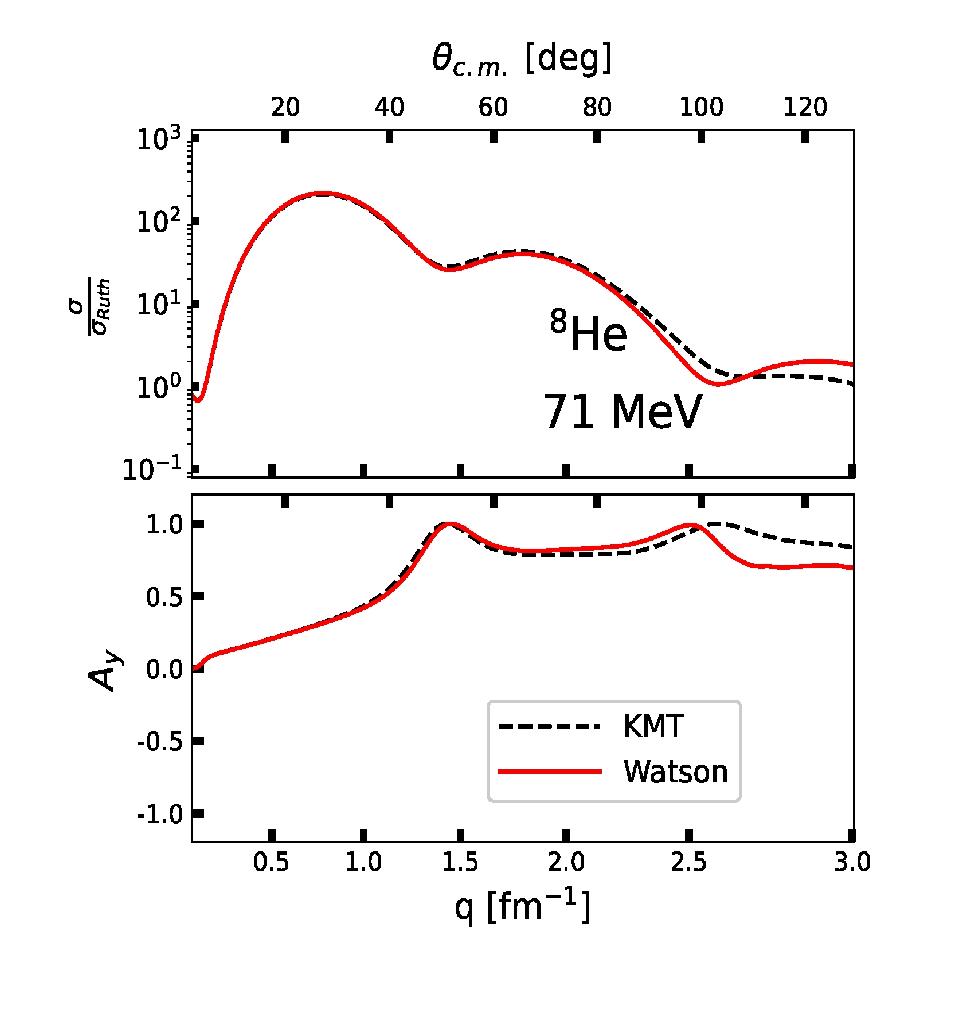
Figure 1: The angular distribution of the differential cross section divided by the Rutherford cross section (upper panel) and the analyzing power ($A_{y}$) for elastic proton scattering from ⁸He at 71 MeV laboratory kinetic energy as function of the momentum transfer $q$ and the c. m. angle calculated with the LENPIC SCS chiral interaction Epelbaum et al. (2015b) with a cutoff $R=1$ fm. The calculations are based on nonlocal densities using $\hbar\Omega=14$ MeV at $N_{\rm max}=14$. The solid (red) line stands for using the Watson optical potential while the black (dashed) line represents the KMT prescription.

If the projectile-target-nucleon interaction is assumed to be the same for all target nucleons and if iso-spin effects are neglected then the KMT approximation ($\frac{A-1}{A}\langle\Phi_{0}|\hat{\tau_{i}}|\Phi_{0}\rangle)$ can be derived from the leading-order Watson potential Kerman et al. (1959). When working with momentum space integral equations, the numerical implementation of Eq. (11) is straightforward Chinn et al. (1993a); Burrows et al. (2019, 2020); Vorabbi et al. (2022). Working in coordinate space with differential equations does not allow an equally straightforward implementation, and thus the KMT prescription is the most favorable alternative. A comparison between leading-order Watson potential and the KMT prescription is shown in Fig. 1 for elastic proton scattering from ⁸He at 71 MeV laboratory kinetic energy. Despite the relatively large difference between the proton and neutron densities for this nucleus the KMT prescription agrees with the exact Watson description very well up to momentum transfers of about 2 fm^-1.

Since Eq. (11) is a one-body integral equation, the principal problem is to find a solution of Eq. (12), which due to many-body character of $G_{0}(E)$ is still a many-body integral equation, and in fact no more easily solved than the starting point of Eq. (1).

For most practical calculations the so-called closure approximation to $G_{0}(E)$ is implemented Miller et al. (1978) turning Eq. (12) into a one-body integral equation. This approximation replaces $H_{A}$ by a constant that is interpreted as an average excitation energy, and is justified when the projectile energy is large compared to typical excitation energies of the nucleus. The closure approximation is very successfully applied for elastic scattering around 80 MeV and higher.

Going beyond the closure approximation in the spirit of the spectator expansion we want to single out one target nucleon $i$ and write $G_{0}(E)$ as

$$G_{0}(E) = (E-h_{0}-H_{A}+i\varepsilon)^{-1}$$ (13)

$$= (E-h_{0}-h_{i}-\sum_{j\neq i}v_{ij}-H^{i}+i\varepsilon)^{-1},$$

where the target Hamiltonian is expanded as $H_{A}=h_{i}+\sum_{j\neq i}v_{ij}+H^{i}$ with $v_{ij}$ being the interaction between target nucleons $i$ and $j$, and $H^{i}$ being an (A-1)-body operator containing all higher order effects. Realizing that $\sum_{j\neq i}v_{ij}\equiv W_{i}$ and thus $H^{i}=H_{A}-h_{i}-W_{i}$ does not have an explicit dependence on the $i$th particle, then $H^{i}$ may be replaced by an average energy $E^{i}$ which is akin to the effective binding energy between the $i$th nucleon and the $A-1$ spectator. This is not an approximation since $G_{0}(E)$ may be regarded as

$$G_{0}(E)=[(E-E^{i})-h_{0}-h_{i}-W_{i}-(H^{i}-E^{i})+i\varepsilon]^{-1}$$ (14)

and $(H^{i}-E^{i})$ should be set aside to be treated in the next order of the expansion of the propagator $G_{0}(E)$. In this order of the expansion $G_{0}(E)$ becomes

$$G_{i}(E)=[(E-E^{i})-h_{0}-h_{i}-W_{i}+i\varepsilon]^{-1},$$ (15)

and Eq. (12) reads

$$\hat{\tau_{i}}=v_{0i}+v_{0i}G_{i}(E)\hat{\tau_{i}}.$$ (16)

In order to connect the above expression with the free NN amplitude

$$t_{0i}=v_{0i}+v_{0i}g_{i}t_{0i}$$ (17)

with

$$g_{i}=[(E-E^{i})-h_{0}-h_{i}+i\varepsilon]^{-1}.$$ (18)

algebraic relations between the resolvents lead to

$$\hat{\tau_{i}}=t_{0i}+t_{0i}G_{i}W_{i}g_{i}(E)\hat{\tau_{i}}.$$ (19)

Defining $G_{i}W_{i}=g_{i}{\mathcal{T}}_{i}$ with ${\mathcal{T}}_{i}=W_{i}+W_{i}g_{i}{\mathcal{T}}_{i}$ leads to

$$\hat{\tau_{i}}=t_{0i}+t_{0i}g_{i}{\mathcal{T}}_{i}g_{i}\hat{\tau_{i}}.$$ (20)

The three-body character of the above expression becomes more evident if one defines it as a set of coupled equations as

$$\hat{\tau_{i}} = t_{0i}+t_{0i}g_{i}X_{i}$$

$$X_{i} = {\mathcal{T}}_{i}g_{i}\hat{\tau_{i}}.$$ (21)

Though the spectator expansion of the operator $U$ in terms of active particles is defined in Eq. (9), we see that this expansion is performed in terms of quantities which contain many-body propagators. Each of the ingredients $\tau_{i}$, $\tau_{ij}$, etc. may themselves be expanded in a spectator expansion, i.e. expanding the many-body propagator also according to the number of active participants. The corrections to the propagator in the leading-order term of $U$ contributions that arise from the $Q$ space, whereas the terms arising from the propagator remain in the $P$ space at first order level. Thus their contribution may be more relevant for elastic scattering.

In an explicit treatment of $G_{i}(E)$ it is necessary to consider the explicit form of $\sum_{j\neq i}v_{ij}=W_{i}$, which is a priori a two-body operator. In the framework of ab initio nuclear structure calculations this will involve two-body densities. In earlier work Chinn et al. (1995a, 1993b, b) the quantity $W_{i}$ was treated as one-body operator, specifically a mean-field potential. This was a physically reasonable choice, though being outside the strict demands of the spectator expansion. However, those studies revealed that the next order in the propagator expansion has little effect on elastic scattering observables at energies larger than 100 MeV, while the description of differential cross section and spin-observables for elastic scattering from ⁴⁰Ca at 48 MeV showed considerable improvement with respect to experiment Chinn et al. (1993b). Obviously this type of calculation will need to be explored within an ab initio approach. In Ref. Chinn et al. (1993b) the energy $E^{i}$ of Eq. (18) was set to zero.

As illustrated in this section, deriving a multiple scattering expansion for elastic NA scattering means projecting on the ground state of the target in order to obtain a Lippman-Schwinger type equation for the transition amplitude and obtaining an operator $U$ for the effective interaction, which is defined in the space $Q=1-P$. In this spirit, the spectator expansion contains therefore two pieces, namely the expansion of the operator $U$ in terms of active particles in the scattering process as well as the expansion of target Hamiltonian $H_{A}$ in the propagator $G_{0}(E)$ in a similar fashion. Thus it is very difficult to define a single expansion parameter which governs the convergence of the expansion.

III Leading order ab initio optical potential based on a chiral NN interaction

The leading order of the spectator expansion involves two active nucleons, the projectile and a target nucleon. Therefore, the leading order is driven by the NN amplitude $\overline{M}$ , which in its most general form can be parameterized in terms of Wolfenstein amplitudes Wolfenstein and Ashkin (1952); Fachruddin et al. (2000); Golak et al. (2010),

$$\overline{M}(\bm{q},\bm{\mathcal{K}}_{NN},\epsilon) = A(\bm{q},\bm{\mathcal{K}}_{NN},\epsilon)\textbf{1}\otimes\textbf{1}$$ (22)

$$+ iC(\bm{q},\bm{\mathcal{K}}_{NN},\epsilon)~{}\left(\bm{\sigma^{(0)}}\cdot\hat{\bm{n}}\right)\otimes\textbf{1}$$

$$+ iC(\bm{q},\bm{\mathcal{K}}_{NN},\epsilon)~{}\textbf{1}\otimes\left(\bm{\sigma^{(i)}}\cdot\hat{\bm{n}}\right)$$

$$+ M(\bm{q},\bm{\mathcal{K}}_{NN},\epsilon)(\bm{\sigma^{(0)}}\cdot\hat{\bm{n}})\otimes(\bm{\sigma^{(i)}}\cdot\hat{\bm{n}})$$

$$+ \left[G(\bm{q},\bm{\mathcal{K}}_{NN},\epsilon)-H(\bm{q},\bm{\mathcal{K}}_{NN},\epsilon)\right](\bm{\sigma^{(0)}}\cdot\hat{\bm{q}})\otimes(\bm{\sigma^{(i)}}\cdot\hat{\bm{q}})$$

$$+ \left[G(\bm{q},\bm{\mathcal{K}}_{NN},\epsilon)+H(\bm{q},\bm{\mathcal{K}}_{NN},\epsilon)\right](\bm{\sigma^{(0)}}\cdot\hat{\bm{\mathcal{K}}})\otimes(\bm{\sigma^{(i)}}\cdot\hat{\bm{\mathcal{K}}})$$ (23)

$$+ D(\bm{q},\bm{\mathcal{K}}_{NN},\epsilon)\left[(\bm{\sigma^{(0)}}\cdot\hat{\bm{q}})\otimes(\bm{\sigma^{(i)}}\cdot\hat{\bm{\mathcal{K}}})+(\bm{\sigma^{(0)}}\cdot\hat{\bm{\mathcal{K}}})\otimes(\bm{\sigma^{(i)}}\cdot\hat{\bm{q}})\right]~{},$$ (24)

where $\bm{\sigma^{(0)}}$ describes the spin of the projectile, and $\bm{\sigma^{(i)}}$ the spin of the struck nucleon. The average momentum in the NN frame is defined as $\bm{\mathcal{K}}_{NN}=\frac{1}{2}\left(\bm{k^{\prime}}_{NN}+\bm{k}_{NN}\right)$. The scalar functions $A$, $C$, $M$, $G$, $H$, and $D$ are referred to as Wolfenstein amplitudes and only depend on the scattering momenta and energy. Each term in Eq. (22) has two components, namely a scalar function of two vector momenta and an energy and the coupling between the operators of the projectile and the struck nucleon. The linear independent unit vectors $\hat{\bm{q}}$, $\hat{\bm{\mathcal{K}}}$, and $\hat{\bm{n}}$ are defined in terms of the momentum transfer and the average momentum as

$$\hat{\bm{q}}=\frac{\bm{q}}{\left|\bm{q}\right|}~{}~{},~{}~{}~{}\hat{\bm{\mathcal{K}}}=\frac{\bm{\mathcal{K}}}{\left|\bm{\mathcal{K}}\right|}~{}~{},~{}~{}~{}\hat{\bm{n}}=\frac{\bm{\mathcal{K}}\times\bm{q}}{\left|\bm{\mathcal{K}}\times\bm{q}\right|},$$ (25)

and span the momentum vector space. With the exception of the momentum transfer $\bm{q}$, which is invariant under frame transformation, the vectors in Eq. (25) need to be considered in their respective frame in explicit calculations Burrows et al. (2020); Burrows (2020). For the struck target nucleon the expectation values of the operator ${\bf 1}$ and the scalar products of $\bm{\sigma^{(i)}}$ with the linear independent unit vectors of Eq. (25) need to be evaluated with the ground state wave functions of the respective nucleus when calculating the leading-order NA effective interaction. Evaluating the expectation value of the operator ${\bf 1}$ in the ground state of the nucleus results in the scalar nonlocal, translationally invariant one-body density that has traditionally been used as input to microscopic or ab initio calculations of leading order effective interactions Elster et al. (1997, 1990); Burrows et al. (2019); Gennari et al. (2018). The other operators from Eq. (25), namely $(\bm{\sigma^{(i)}}\cdot\hat{\bm{n}})$, $(\bm{\sigma^{(i)}}\cdot\hat{\bm{q}})$, and $(\bm{\sigma^{(i)}}\cdot\hat{\bm{\mathcal{K}}})$ need to also be evaluated for a leading-order ab initio NA effective interaction, in which the NN interaction is treated on equal footing in the reaction and structure calculation.

Thus, the general expression for a nonlocal density needs to include the spin operator $\bm{\sigma^{(i)}}$ explicitly,

$$\rho^{K_{s}}_{q_{s}}\left(\bm{p},\bm{p}^{\prime}\right)=\left\langle\Phi_{0}^{\prime}\left|\sum_{i=1}^{A}\delta^{3}(\bm{p_{i}}-\bm{p})\delta^{3}(\bm{p_{i}}^{\prime}-\bm{p}^{\prime})\sigma_{q_{s}}^{(i)K_{s}}\right|\Phi_{0}\right\rangle~{},$$ (26)

where $\sigma^{(i)K_{s}}_{q_{s}}$ is the spherical representation of the spin operator and the wavefunction $\Phi_{0}$ $(\bm{p_{1}},...,\bm{p_{A}})=\left\langle\bm{p_{1}},...,\bm{p_{A}}|\Phi_{0}\right\rangle$ is defined in momentum space. Evaluating this expression for $K_{s}=0$ gives the nonlocal one-body scalar density and $K_{s}=1$ becomes a nonlocal one-body spin density.

The Wolfenstein parameterization of Eq. (22) requires the evaluation of scalar products of the one-body spin density with unit momentum vectors. Since those only depend on the momenta $\bm{p}$ and $\bm{p}^{\prime}$, those can be calculated as $\rho^{K_{s}}\left(\bm{p},\bm{p}^{\prime}\right)\cdot\hat{\bm{n}}$, $\rho^{K_{s}}\left(\bm{p},\bm{p}^{\prime}\right)\cdot\hat{\bm{q}}$, and $\rho^{K_{s}}\left(\bm{p},\bm{p}^{\prime}\right)\cdot\hat{\bm{\mathcal{K}}}$. For the explicit calculation of $\rho^{K_{s}}\left(\bm{p},\bm{p}^{\prime}\right)\cdot\hat{\bm{n}}$, we refer the reader to Burrows et al. (2020); Burrows (2020). The scalar products $(\bm{\sigma^{(i)}}\cdot\hat{\bm{q}})$ and $(\bm{\sigma^{(i)}}\cdot\hat{\bm{\mathcal{K}}})$ represent scalar products of a pseudo-vector and a vector, a construct that is not invariant under parity transformations, and thus vanish when sandwiched between ground state wave functions, which is explicitly shown in Burrows (2020). Thus the tensor contributions of the NN force only enter the leading order effective NA interaction through the Wolfenstein amplitude $M$ as long as elastic scattering is considered. When e.g. transition amplitudes between states of different parity would be considered, the other tensor amplitudes will contribute.

Currently contributions to elastic scattering observables due to the spin-projected one-body densities have only been calculated for light nuclei with $0^{+}$ ground states, and it was found that this contribution is very small for nuclei with equal proton and neutron numbers Burrows et al. (2020); Baker et al. (2021). This is likely different for nuclei with ground states of nonzero spin, which was explored for ¹⁰B polarization transfer observables in Ref. Cunningham et al. (2011, 2013), where the authors assume a nuclear structure which consists of a core and valence nucleons. The work of Ref. Vorabbi et al. (2022) extends the standard leading order calculation to nonzero spin nuclei, however does not consider the inherent tensor contributions from the NN force in their formulation. This leaves the importance of a consistent treatment of the NN force on elastic scattering from nonzero spin nuclei still an open question.

The complete calculation of the leading-order effective interaction describing the scattering of a proton from a nucleus in a $0^{+}$ ground state and which enters the integral Eq. (11) as driving term is given by

$$\widehat{U}_{\mathrm{p}}(\bm{q},\bm{\mathcal{K}}_{NA},\epsilon)=$$ (28)

$$\sum_{\alpha=\mathrm{n,p}}\int d^{3}{\mathcal{K}}\eta\left(\bm{q},\bm{\mathcal{K}},\bm{\mathcal{K}}_{NA}\right)A_{\mathrm{p}\alpha}\left(\bm{q},\frac{1}{2}\left(\frac{A+1}{A}\bm{\mathcal{K}}_{NA}-\bm{\mathcal{K}}\right);\epsilon\right)\rho_{\alpha}^{K_{s}=0}\left(\bm{\mathcal{P}^{\prime}},\bm{\mathcal{P}}\right)$$

$$+ i(\bm{\sigma^{(0)}}\cdot\hat{\bm{n}})\sum_{\alpha=\mathrm{n,p}}\int d^{3}{\mathcal{K}}\eta\left(\bm{q},\bm{\mathcal{K}},\bm{\mathcal{K}}_{NA}\right)C_{\mathrm{p}\alpha}\left(\bm{q},\frac{1}{2}\left(\frac{A+1}{A}\bm{\mathcal{K}}_{NA}-\bm{\mathcal{K}}\right);\epsilon\right)\rho_{\alpha}^{K_{s}=0}\left(\bm{\mathcal{P}^{\prime}},\bm{\mathcal{P}}\right)$$ (29)

$$+ i\sum_{\alpha=\mathrm{n,p}}\int d^{3}{\mathcal{K}}\eta\left(\bm{q},\bm{\mathcal{K}},\bm{\mathcal{K}}_{NA}\right)C_{\mathrm{p}\alpha}\left(\bm{q},\frac{1}{2}\left(\frac{A+1}{A}\bm{\mathcal{K}}_{NA}-\bm{\mathcal{K}}\right);\epsilon\right)S_{n,\alpha}\left(\bm{\mathcal{P}^{\prime}},\bm{\mathcal{P}}\right)\cos\beta$$

$$+ i(\bm{\sigma^{(0)}}\cdot\hat{\bm{n}})\sum_{\alpha=\mathrm{n,p}}\int d^{3}{\mathcal{K}}\eta\left(\bm{q},\bm{\mathcal{K}},\bm{\mathcal{K}}_{NA}\right)(-i)M_{\mathrm{p}\alpha}\left(\bm{q},\frac{1}{2}\left(\frac{A+1}{A}\bm{\mathcal{K}}_{NA}-\bm{\mathcal{K}}\right);\epsilon\right)S_{n,\alpha}\left(\bm{\mathcal{P}^{\prime}},\bm{\mathcal{P}}\right)\cos\beta.$$

The term $\eta\left(\bm{q},\bm{\mathcal{K}},\bm{\mathcal{K}_{NA}}\right)$ is the Møller factor Møller (1945) describing the transformation from the NN frame to the NA frame. The functions $A_{\mathrm{p}\alpha}$, $C_{\mathrm{p}\alpha}$, and $M_{\mathrm{p}\alpha}$ represent the NN interaction through Wolfenstein amplitudes Wolfenstein and Ashkin (1952). Since the incoming proton can interact with either a proton or a neutron in the nucleus, the index $\alpha$ indicates the neutron ($\mathrm{n}$) and proton ($\mathrm{p}$) contributions, which are calculated separately and then summed up. With respect to the nucleus, the operator $i(\bm{\sigma^{(0)}}\cdot\hat{\bm{n}})$ represents the spin-orbit operator in momentum space with respect to the projectile. As such, Eq. (28) exhibits the expected form of an interaction between a spin-$\frac{1}{2}$ projectile and a target nucleus in a $J=0$ state Rodberg and Thaler (1967). The momentum variables in the problem are given as

$$\bm{q} = \bm{p^{\prime}}-\bm{p}=\bm{k^{\prime}}-\bm{k},$$ (31)

$$\bm{\mathcal{K}} = \frac{1}{2}\left(\bm{p^{\prime}}+\bm{p}\right),$$ (32)

$$\bm{\mathcal{K}_{NA}} = \frac{A}{A+1}\left[\left(\bm{k^{\prime}}+\bm{k}\right)+\frac{1}{2}\left(\bm{p^{\prime}}+\bm{p}\right)\right],$$ (33)

$$\bm{\mathcal{P}} = \bm{\mathcal{K}}+\frac{A-1}{A}\frac{\bm{q}}{2},$$ (34)

$$\bm{\mathcal{P^{\prime}}} = \bm{\mathcal{K}}-\frac{A-1}{A}\frac{\bm{q}}{2}.$$

The two quantities representing the structure of the nucleus are the scalar one-body density $\rho_{\alpha}^{K_{s}=0}\left(\bm{\mathcal{P}^{\prime}},\bm{\mathcal{P}}\right)$ and the spin-projected momentum distribution $S_{n,\alpha}\left(\bm{\mathcal{P}^{\prime}},\bm{\mathcal{P}}\right)=\rho^{K_{s}=1}\left(\bm{\mathcal{P}^{\prime}},\bm{\mathcal{P}}\right)\cdot\bm{\hat{n}}$. Both distributions are nonlocal and translationally invariant. The reduced matrix elements entering the one-body densities are obtained within the NCSM (SA-NCSM) in the center-of-mass frame of the nucleus. In order to employ them in calculating the leading-order effective NA interaction, this center-of-mass variable must be removed. Within the framework of NCSM (SA-NCSM) the technique for obtaining nonlocal and translationally invariant one-body densities is well developed Navratil (2004); Cockrell et al. (2012); Mihaila and Heisenberg (1999); Gennari et al. (2018); Burrows et al. (2019); Navratil (2021). Lastly, the term $\cos\beta$ in Eq. (28) results from projecting $\bm{\hat{n}}$ from the NN frame to the NA frame. For further details, see Ref. Burrows et al. (2020).

IV Chiral Truncation uncertainties in the leading order optical potential

With the emergence of nuclear forces based on chiral effective field theory (EFT), we are presented with an opportunity to study the nucleon-nucleus effective interaction as it develops order-by-order in a chiral EFT framework. Given the hierarchical nature of chiral EFT, we can combine these order-by-order results to reliably estimate truncation uncertainties associated with the higher chiral orders not included in the calculations. To this end, Refs. Melendez et al. (2017, 2019); Epelbaum et al. (2020) first implemented uncertainty quantification for the cases of NN and Nd scattering by assuming a quantity $y(x)$ at a chiral order $k$ can be written as

$$y_{k}(x)=y_{\mathrm{ref}}(x)\sum_{n=0}^{k}c_{n}(x)Q^{n}(x)$$ (35)

where $y_{\mathrm{ref}}(x)$ is a reference value that sets the scale of the problem and also includes the dimensions of the quantity $y(x)$ of interest. By construction, the coefficients $c_{n}(x)$ are dimensionless and are expected to be of order unity. The remaining quantity $Q(x)$ is the expansion parameter associated with the chiral EFT. The expansion parameter is usually defined as

$$Q=\frac{1}{\Lambda_{b}}\max(M_{\pi},p)$$ (36)

where $\Lambda_{b}$ is the breakdown scale of the EFT, $M_{\pi}$ is the pion mass, and $p$ is the relevant momentum for the problem. Various works Melendez et al. (2017, 2019); Epelbaum et al. (2020) have identified the relevant momentum in different ways, but keeping with Ref. Baker et al. (2022) we choose the relevant momentum as the center-of-mass (c.m.) momentum in the nucleon-nucleus system

$$p^{2}_{NA}=\frac{E_{\mathrm{lab}}A^{2}m^{2}(E_{\mathrm{lab}}+2m)}{m^{2}(A+1)^{2}+2AmE_{\mathrm{lab}}}$$ (37)

where $E_{\mathrm{lab}}$ is the kinetic energy of the projectile in the laboratory frame, $A$ is the target nucleus’s mass number, and $m$ is the mass of the nucleon.

Previous scattering works Melendez et al. (2019); Baker et al. (2022) have noted that various results indicate, when identifying the relevant momentum, the momentum transfer $q$ should also be considered. That is, the expansion parameter would be more appropriately defined as

$$Q=\frac{1}{\Lambda_{b}}\max(M_{\pi},p_{NA},q)$$ (38)

The momentum transfer in elastic scattering is defined as

$$q=2p_{NA}\sin\left(\frac{\theta_{\mathrm{c.m.}}}{2}\right)$$ (39)

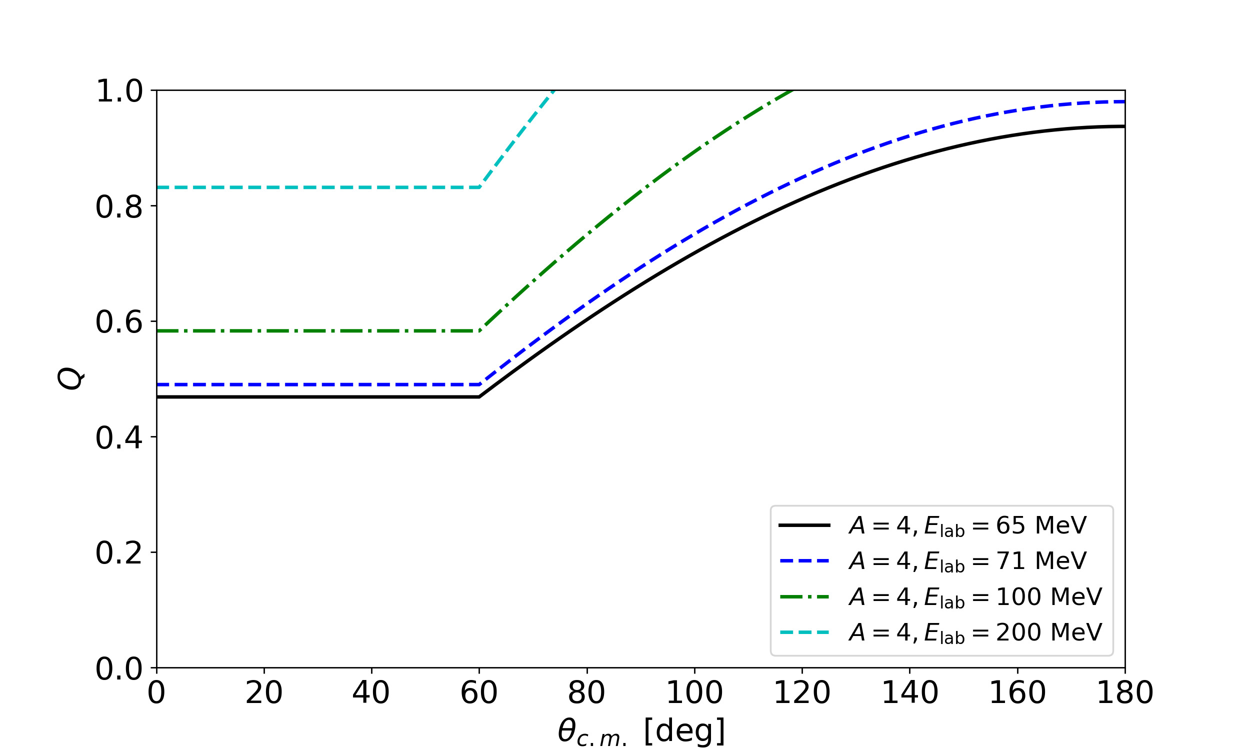
Figure 2: The expansion parameter $Q$, defined by Eq. (38) where $\Lambda_{b}=600$ MeV, as a function of the center-of-mass angle $\theta_{\mathrm{c.m.}}$ for a range of lab projectile energies $E_{\mathrm{lab}}$. In this case of nucleon-nucleus (NA) elastic scattering, the transition between when the expansion parameter is dominated by the center-of-mass momentum and the momentum transfer can easily be identified.

where $\theta_{\mathrm{c.m.}}$ is the scattering angle in the c.m. frame. Notably, including the momentum transfer in Eq. (38) makes the expansion parameter a function of $\theta_{\mathrm{c.m.}}$, even though the other momentum scales in Eq. (38) are independent of the scattering angle. When considering observables such as the differential cross section or analyzing power that are functions of $\theta_{\mathrm{c.m.}}$, this implies the expansion parameter will be larger at backward angles than at forward angles. Furthermore, since the leading order of the spectator expansion is not applicable at low energies, we only consider scattering at lab energies of 65 MeV or higher. As a result, the chiral expansion parameter becomes $Q=\max(p_{NA},q)/\Lambda_{b}$. This expansion parameter is shown in Fig. 2 for the case of $A=4$ and $\Lambda_{b}=600$ MeV. Because of the factorization of the c.m. momentum, there is a universal scattering angle at which the momentum transfer $q$ begins to dominate the expansion parameter, regardless of the chosen $E_{\mathrm{lab}}$ or nucleus. We will exploit this behavior in later sections.

IV.1 Nuclear structure calculations

Prior to our detailed study of truncation uncertainties of a chiral NN interaction in elastic NA scattering observables we need to choose a specific chiral NN interaction. Here we want to focus on the EKM chiral NN interaction Epelbaum et al. (2015a, b) with a semi-local coordinate space regulator of R = 1 fm, which has a breakdown scale of $\Lambda_{b}$ = 600 MeV. This interaction gives a slightly better description of the ground state energies in the upper $p$-shell than a similar, more recent interaction with a semi-local momentum space regulator. For consistency with the leading-order optical we only use the NN potentials, omitting three-nucleon forces, which appear at N2LO in the chiral expansion, both in the structure and the scattering part of the calculations. Including three-nucleon forces consistently in both, the structure and scattering calculations requires going beyond the leading-order optical potential, and is beyond the scope of this work. Though initial attempts of incorporating three-nucleon forces as an effective density-dependent NN force in the scattering part have been presented Vorabbi et al. (2021), they can not yet be considered as systematic consideration of three-nucleon forces in NA scattering. For similar reasons, we restrict most of our results to N2LO since three-nucleon force contributions at N3LO and N4LO are significant Binder et al. (2016).

Next, the translationally-invariant one-body density needed for the scattering calculation can be obtained using the NCSM approach, in which the nuclear wavefunction is expanded in Slater determinants of harmonic oscillator basis functions Barrett et al. (2013). Ideally, one uses a sufficiently large basis to ensure convergence of this expansion, but in practice observables depend on both the many-body basis truncation, $N_{\mathrm{max}}$ (defined as the total number of harmonic oscillator quanta in the many-body system above the minimal configuration), and on the harmonic oscillator scale $\hbar\Omega$. In Table 1 we give the ground state binding energies and point-proton radii of ⁴He, ¹²C, and ¹⁶O obtained with the EKM chiral NN potential Epelbaum et al. (2015a, b) with a semi-local coordinate space regulator of R = 1 fm (note that at N2LO we did not include any three-nucleon forces).

For ⁴He we can obtain nearly converged results for both the binding energy and the proton radius, and these results agree, to within their estimated numerical uncertainties (the first set of uncertainties in Table 1), with Yakubovsky calculations using the same NN potential Binder et al. (2016). However, for larger nuclei such as ¹²C and ¹⁶O we are more limited in the $N_{\mathrm{max}}$ values that can be reached on current computational resources. 

IV.2 Pointwise truncation uncertainties

To assess the relative size of chiral truncation uncertainties compared to other known uncertainties, e.g. the harmonic oscillator parameters $N_{\mathrm{max}}$ and $\hbar\Omega$, we employ a pointwise truncation procedure and study reaction observables that are not functional quantities, e.g. reaction cross sections at a specified laboratory energy. This pointwise approach was previously implemented in Refs. Melendez et al. (2019); Baker et al. (2022) and it starts by assuming the expansion parameter $Q$ and reference scale $y_{\mathrm{ref}}$ are known. From there, we can apply Eq. (35) to calculate the coefficients $c_{n}$, which are treated as independent draws from the same underlying distribution. The properties of this distribution can be learned from Bayesian techniques and the posterior distribution for the prediction can be readily calculated with its associated credible intervals. For more details, see Ref. Melendez et al. (2019).

In order to estimate the chiral truncation uncertainties of the obtained ground state binding energies and radii, we apply the pointwise approach with $Q\approx 0.3$ as the effective expansion parameter, following Ref. Binder et al. (2018). These uncertainties are listed as the second set of uncertainties in Table 1, starting from NLO. Here we see that for the energies, the chiral uncertainties are at least of the same order as the estimated numerical uncertainties; however, the uncertainties of the radii of ¹²C and ¹⁶O are clearly dominated by their systematic dependence on the basis parameter $\hbar\Omega$.

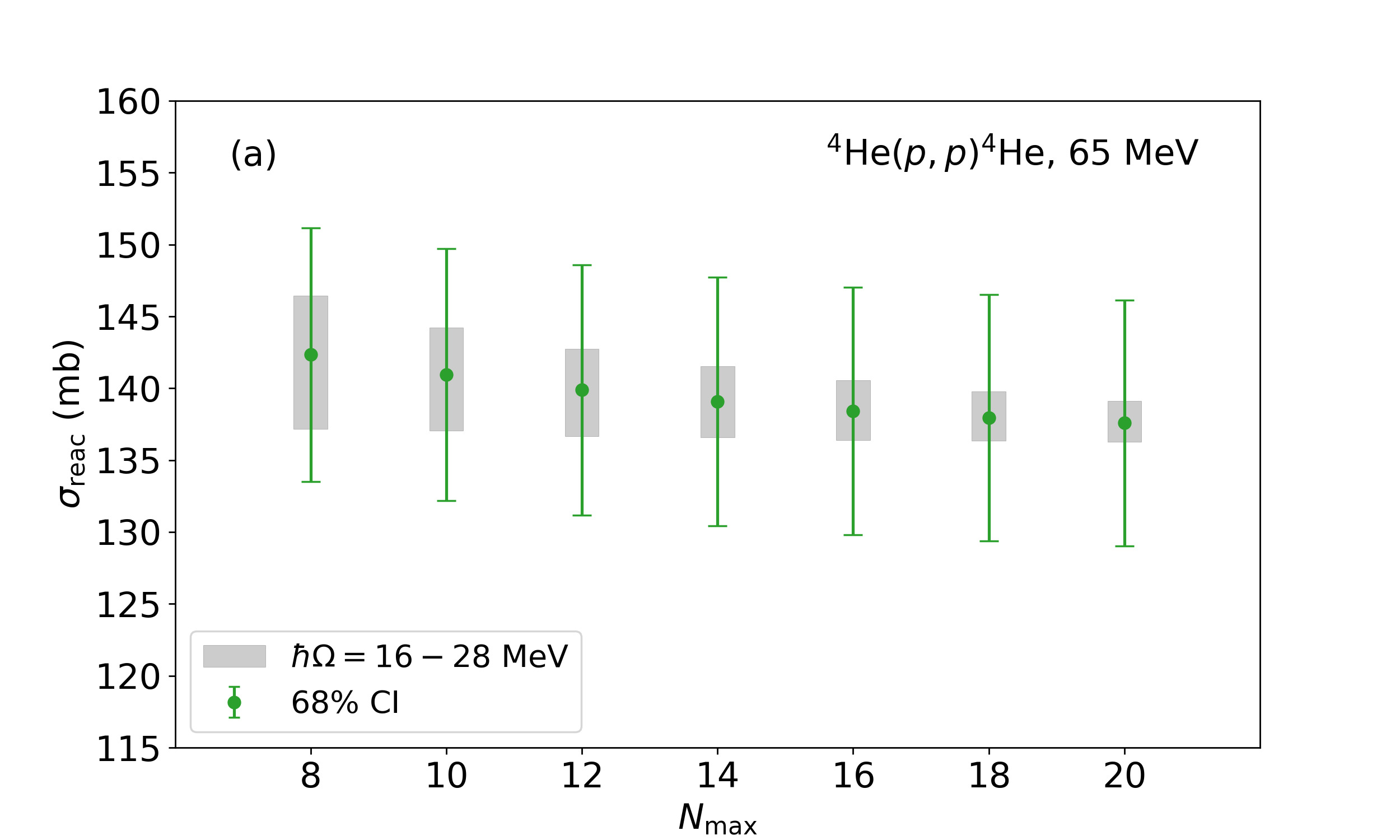
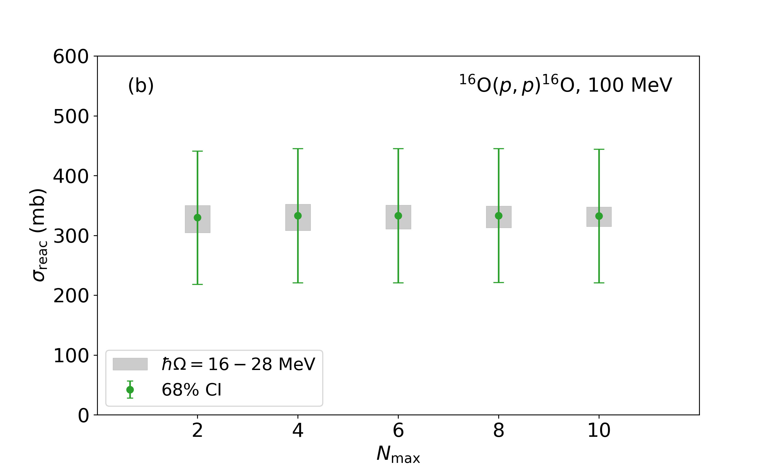
Figure 3: Reaction cross section for proton scattering on (a) ⁴He at 65 MeV and (b) ¹⁶O at 100 MeV, both at N2LO as a function of $N_{\mathrm{max}}$. The error bars show a 68% credible interval (CI) from using a pointwise error estimation with the LO, NLO, and N2LO results. The shaded regions show variations with respect to the harmonic oscillator parameter $\hbar\Omega$. The values of the expansion parameters used were $Q=0.47$ for⁴He at 65 MeV and $Q=0.69$ for ¹⁶O at 100 MeV. Note the different scales in (a) and (b).

To illustrate the pointwise approach for scattering observables, Fig. 3 shows the reaction cross sections for proton scattering from ⁴He at 65 MeV and ¹⁶O at 100 MeV. For each case, the result is shown as a function of $N_{\mathrm{max}}$, and variations with respect to $\hbar\Omega$ are indicated. While more obvious for the smaller nucleus where the NCSM can better converge, in both cases the uncertainty resulting from the chiral truncation remains larger than the uncertainty arising from the many-body method. To better illustrate this point, we present the reaction cross section for ⁴He with a scale starting from 115 mb and with a range of only 45 mb, while using the full range of 600 mb for ¹⁶O. While larger model spaces will better converge the NCSM results, smaller truncation uncertainties will only be achieved by higher chiral orders, despite the noticeable dependence of the radii on the harmonic oscillator parameter $\hbar\Omega$, in particular for the heavier nuclei, in the current calculations. Note however that even at N3LO we anticipate the chiral truncation uncertainties will be larger than the indicated variations with respect to the harmonic oscillator parameter $\hbar\Omega$ due to the rather large value of the expansion parameter $Q$ in the scattering calculation.

IV.3 Correlated truncation uncertainties

For functional quantities $y(x)$ we employ a correlated approach that includes information at nearby values of $x$. This approach is better for observables such as a differential cross section, which we know does not vary wildly from values at nearby angles. It also starts from Eq. (35) and treats the coefficients $c_{n}(x)$ as independent draws from an underlying Gaussian process. This Gaussian process encodes information about the correlation length $\ell$, and the qualities of the underlying distribution can be learned from the order-by-order results. This training is followed up by testing procedures which seek to confirm the Gaussian process has been appropriately fit to the available results, and if not, to diagnose potential issues. From a well-fit Gaussian process we can then extract truncation uncertainties for the functional quantities. For more details and applications, see Refs. Melendez et al. (2019); Baker et al. (2022).

In the following examples, we examine proton scattering for ⁴He, ¹²C, and ¹⁶O at various projectile energies and compare to the available experimental data. In each case, we show the convergence with respect to chiral order and the resulting decrease in the size of the chiral truncation uncertainties, as well as discuss any associated physics insights. To avoid concerns about the expansion parameter increasing at larger angles, we mostly restrict our analysis to forward angles where we expect the expansion parameter to be independent of the scattering angle.

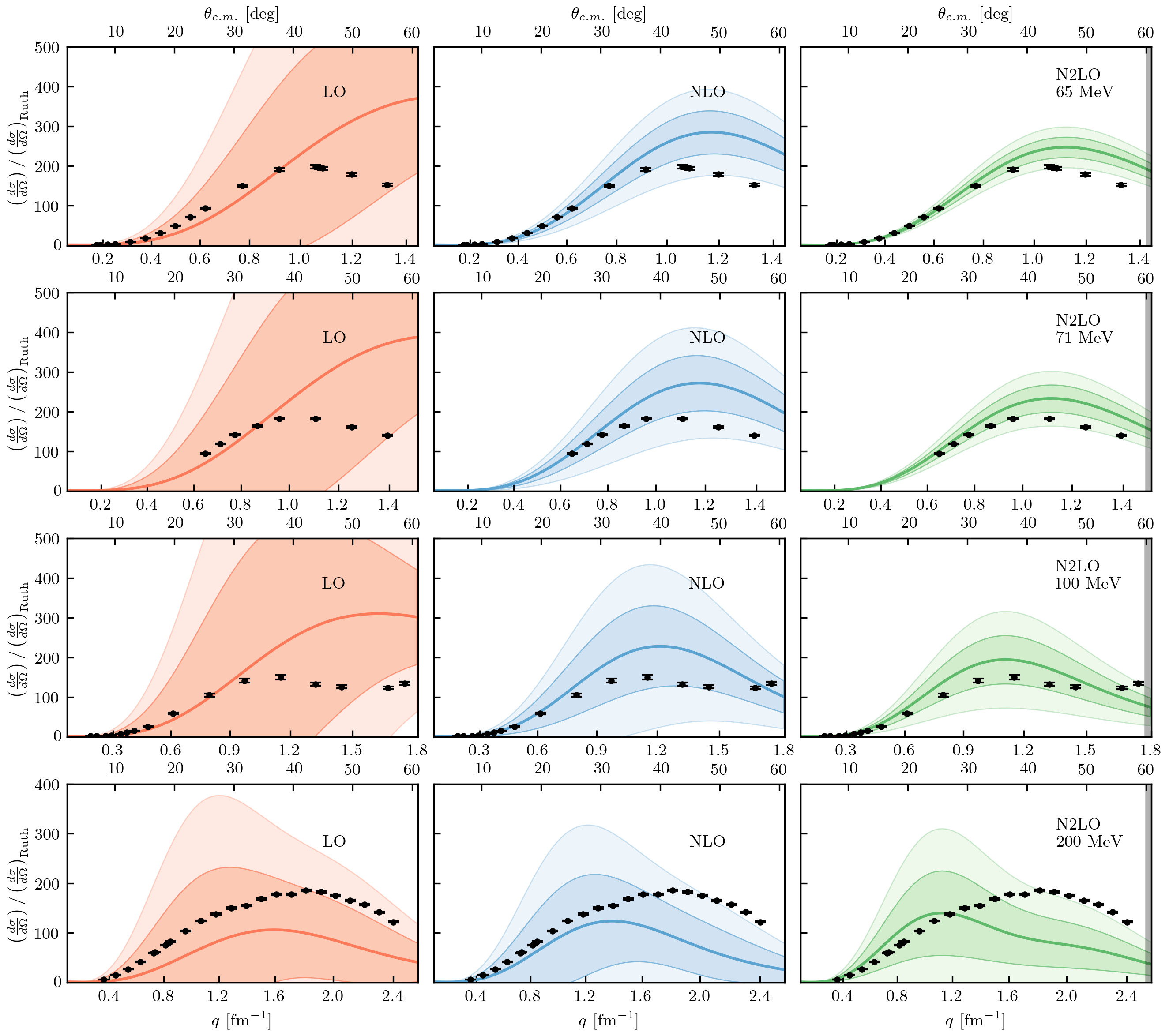
Figure 4: Differential cross section divided by Rutherford for proton scattering on ⁴He at (first row) 65 MeV, (second row) 71 MeV, (third row) 100 MeV, and (fourth row) 200 MeV for LO (left column), NLO (middle column), and N2LO (right column) with corresponding $1\sigma$ (darker bands) and $2\sigma$ (lighter bands) error bands. Black dots are experimental data from Refs. Imai et al. (1979) (65 MeV), Burzynski et al. (1989) (71 MeV), Goldstein et al. (1970) (100 MeV), and Moss et al. (1980) (200 MeV).

For proton scattering on ⁴He, we see good agreement with experiment for the differential cross sections (Fig. 4) at lower projectile energies. Below 100 MeV, most data points fall within the $2\sigma$ uncertainty band, and at 100 MeV a majority of the data points are within the $1\sigma$ band. At the highest energy of 200 MeV, the chosen interaction seems unable to reproduce the experimental data, though this is not uncommon for scattering from ⁴He.

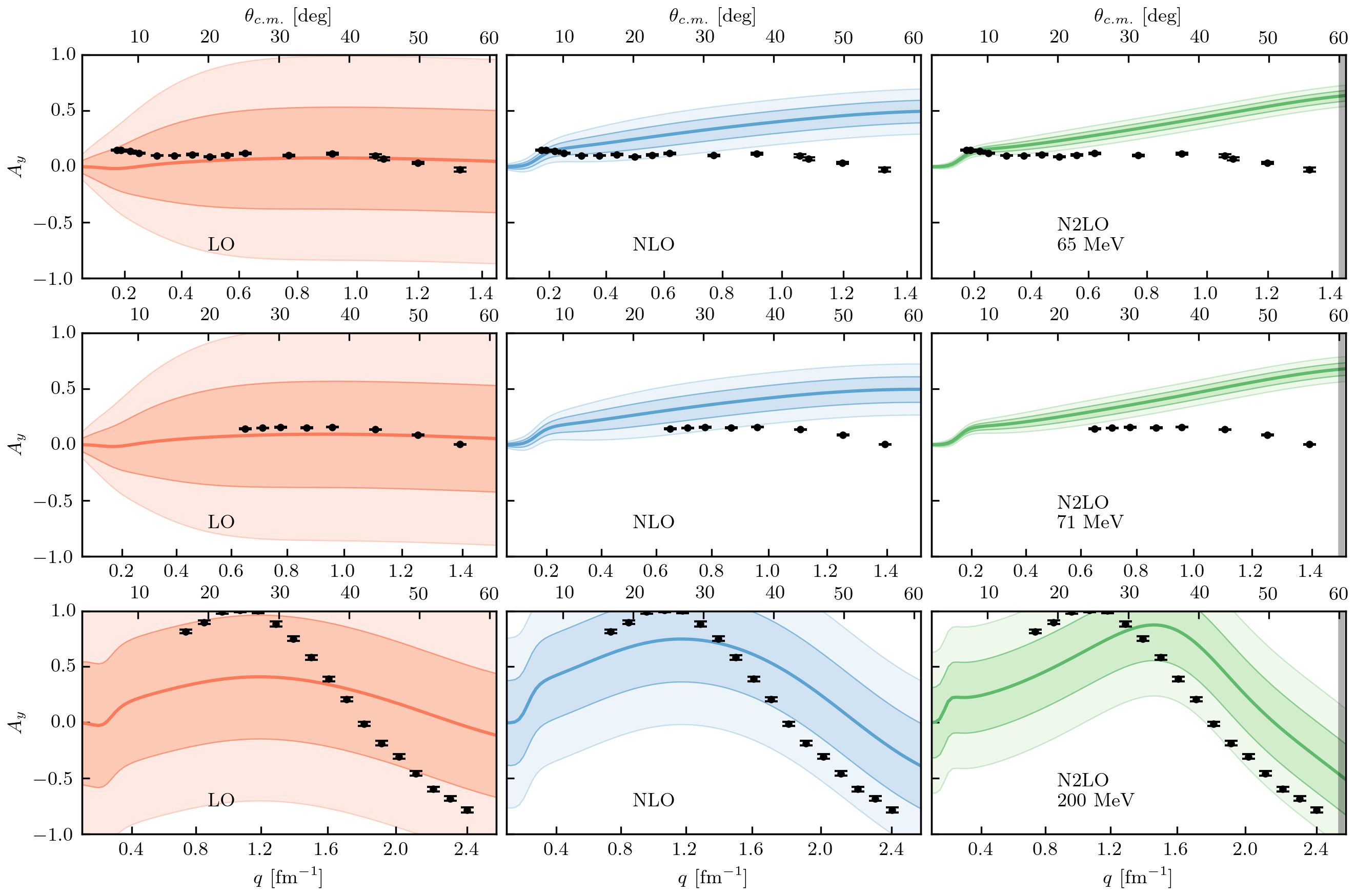
Figure 5: Analyzing power for proton scattering on ⁴He at (first row) 65 MeV, (second row) 71 MeV, and (third row) 200 MeV) for LO (left column), NLO (middle column), and N2LO (right column) with corresponding $1\sigma$ (darker bands) and $2\sigma$ (lighter bands) error bands. Black dots are experimental data from Refs. Imai et al. (1979) (65 MeV), Burzynski et al. (1989) (71 MeV), and Moss et al. (1980) (200 MeV).

The analyzing powers for proton scattering on ⁴He (Fig. 5) is more complicated. For the lower energies of 65 and 71 MeV, the experimental data shows a near zero value, regardless of scattering angle. In the scattering of a spin-1/2 particle from a spin-0 nucleus, this indicates that there is no spin-orbit force at play. This behavior is only reproduced by the LO result, for which the chiral NN interaction only contains the one-pion exchange and contact terms, which do not produce a spin-orbit force. At NLO the two-pion exchange diagrams are responsible for reproducing the NN $p$-waves and thus provide a spin-orbit force that leads to a non-zero value for the analyzing power in NA scattering. At N2LO there are no new terms in the two-nucleon sector, and thus $A_{y}$ does not change its shape at that chiral order. Therefore, one needs to conclude that in this case other physics which goes beyond the leading order NA effective interaction may be needed to describe the analyzing power.

For the higher energy of 200 MeV, all of the experimental data points are within the $2\sigma$ uncertainty band, though there is a slight offset in the shape. In all cases, the analyzing power is more difficult to reproduce using this interaction, though other interactions have done better Burrows et al. (2018, 2020)

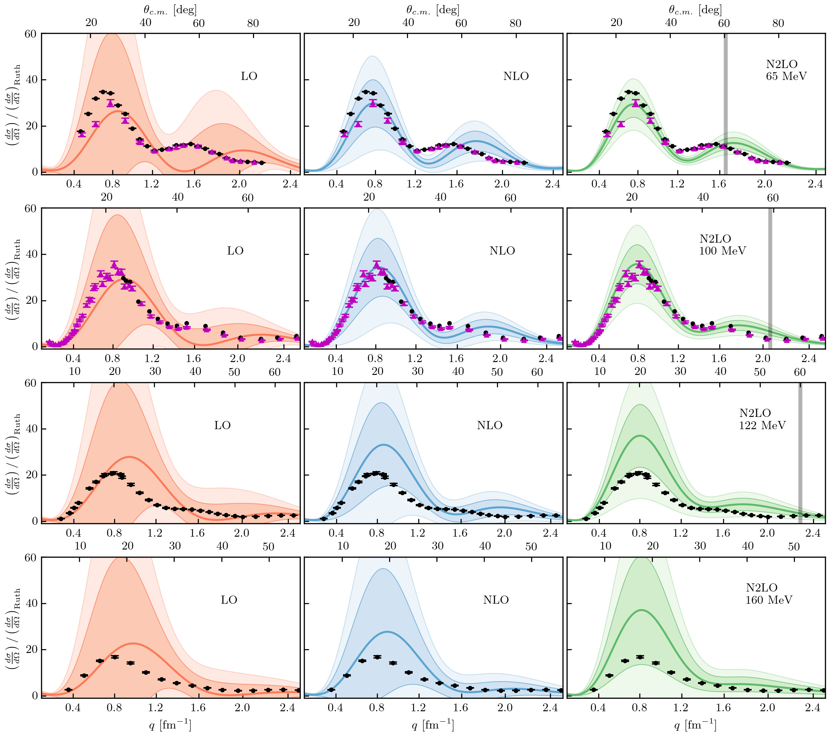
Figure 6: Differential cross section divided by Rutherford for proton scattering on ¹²C at (first row) 65 MeV, (second row) 100 MeV, (third row) 122 MeV, and (fourth row) 160 MeV for LO (left column), NLO (middle column), and N2LO (right column) with corresponding $1\sigma$ (darker bands) and $2\sigma$ (lighter bands) error bands. Black dots/purple triangles are experimental data from Refs. Ieiri et al. (1987a) (65 MeV, black dots), Kato et al. (1985) (65 MeV, purple triangles), Strauch and Titus (1956) (96 MeV, purple triangles), Gerstein et al. (1957) (99 MeV, black dots), and Meyer et al. (1983) (122 MeV and 160 MeV). Figure taken from Ref.Baker et al. (2022).

For proton scattering from ¹²C, the differential cross sections (Fig. 6) are reliably reproduced by the central value of the N2LO calculations up to 100 MeV laboratory kinetic energy, and systematically over-predict at higher energies. As the projectile energy increases, the expansion parameter increases and as a result uncertainty bands become larger. This is most noticeable at 160 MeV: the experimental data is within the $1\sigma$ band, but the size of that band, as well as the $2\sigma$ band, are so large that they are not practically useful. The gray bars in the cross section panels for N2LO indicate the momentum transfer up to where we expect the expansion parameter to be dominated by the c.m. momentum $p_{NA}$. Once the momentum transfer exceeds the value given by the bar, the uncertainty is dominated by the momentum transfer $q$, and is thus underrepresented by the method we use. Note that the vertical bar is at the same scattering angle $\theta_{\mathrm{c.m.}}$, but different momentum transfer $q$, as function of the projectile energy since $p_{NA}$ is a function of the projectile energy as given in Eq. (37). Looking at the lower energies, the increasing agreement with experiment in the first peak and minimum as higher orders in the chiral NN interaction are included gives the correct trend. Minima in the differential cross section correlate with the size of the target nucleus. It is well well known Binder et al. (2018), and also evident from Table 1, that the nuclear binding energy calculated with the LO of the chiral NN interaction is way too large and correspondingly the radius much too small. Only when going to NLO and N2LO the binding energy as well as the radius move into the vicinity of their experimental values. This finding from structure calculations is corroborated by the calculations in Fig. 6, where with increasing chiral order the calculated first diffraction minimum moves towards smaller momentum transfers indicating a larger nuclear size.

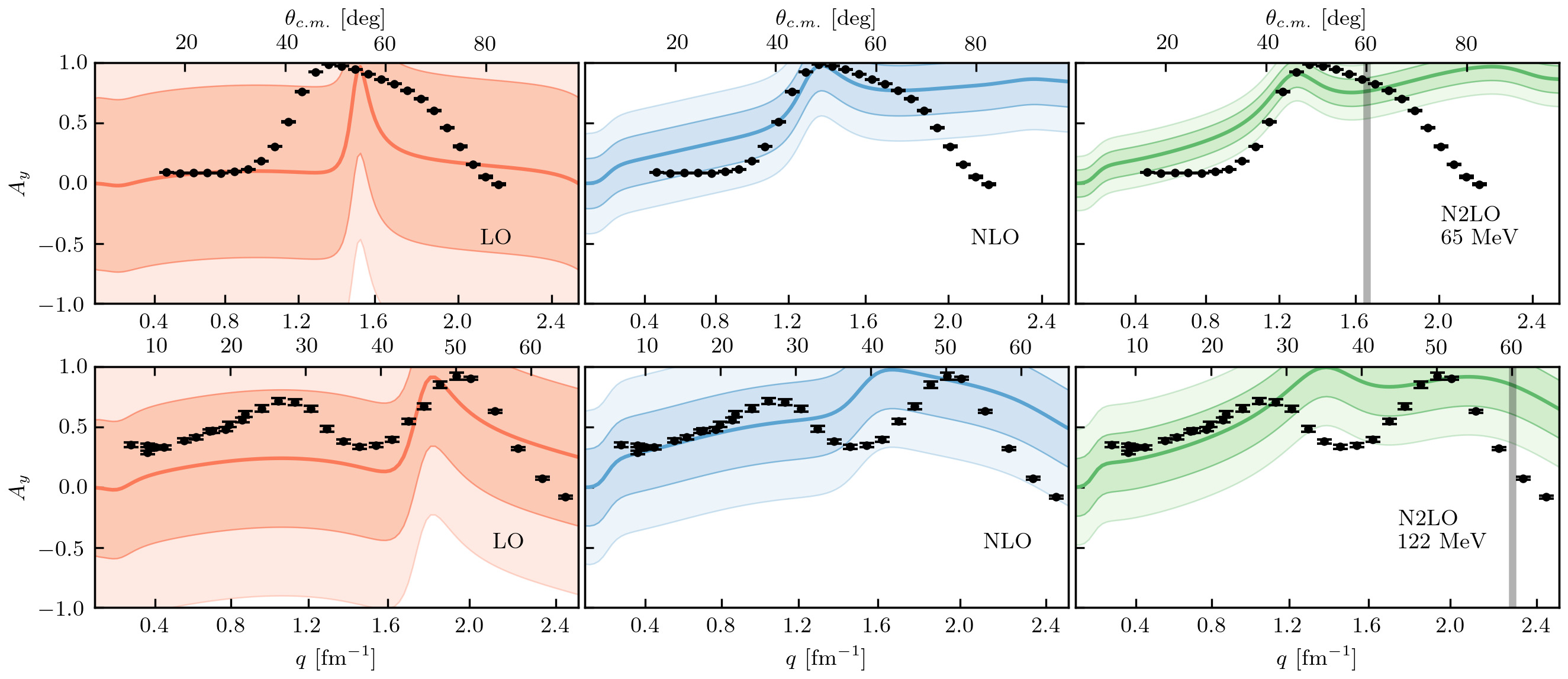
Figure 7: Analyzing power for proton scattering on ¹²C at (first row) 65 MeV and (second row) 122 MeV for LO (left column), NLO (middle column), and N2LO (right column) with corresponding $1\sigma$ (darker bands) and $2\sigma$ (lighter bands) error bands. Black dots are experimental data from Refs. Ieiri et al. (1987b) (65 MeV) and Meyer et al. (1983) (122 MeV). Figure taken from Ref. Baker et al. (2022).

The analyzing powers for proton scattering on ¹²C are at 65 MeV also almost zero for small momentum transfers and rise at $q$ = 1.2 fm^-1 to its maximum value of +1. This is captured by the NLO calculation where spin-contributions occur in the NN interaction (Fig. 7). For 65 MeV, the experimental data is mostly within the $2\sigma$ band until approximately $\theta_{\mathrm{c.m.}}=60^{\circ}$, where we expect the expansion parameter to being increasing and the uncertainty bands to thus be underestimates. For 122 MeV, the very forward direction is inside the $1\sigma$ band, but the overall shape of the experimental data is not well captured by this interaction.

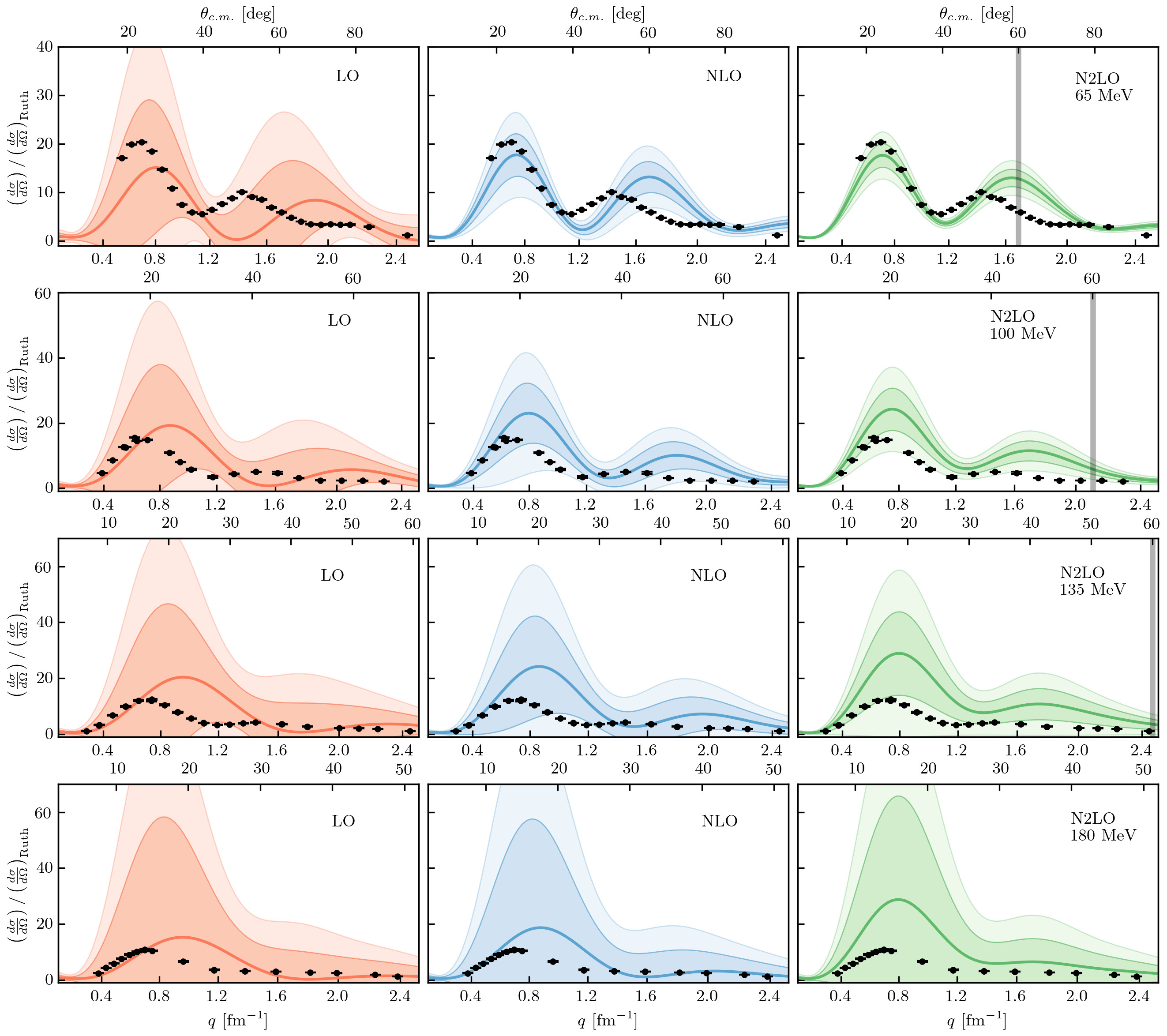
Figure 8: Differential cross section divided by Rutherford for proton scattering on ¹⁶O at (first row) 65 MeV, (second row) 100 MeV, (third row) 135 MeV, and (fourth row) 180 MeV for LO (left column), NLO (middle column), and N2LO (right column) with corresponding $1\sigma$ (darker bands) and $2\sigma$ (lighter bands) error bands. Black dots are experimental data from Refs. Sakaguchi et al. (1979) (65 MeV), Seifert (1990) (100 MeV), Kelly et al. (1989) (135 MeV), and Kelly et al. (1990) (180 MeV). Figure taken from Ref. Baker et al. (2022).

For proton scattering from ¹⁶O, the differential cross sections (Fig. 8) are similar to the ¹²C case. Namely, the lower energies do reasonably well at describing the data within the $2\sigma$ bands, but as the projectile energy increases the uncertainty bands increase to unhelpful sizes. At the lowest energy of 65 MeV, we see a better and better reproduction of the first minimum in the differential cross section as the chiral order increases. Again, this first minimum is known to be related to the size of the nucleus, so this is an important feature to reproduce from both a structure, see Table 1, and reaction perspective.

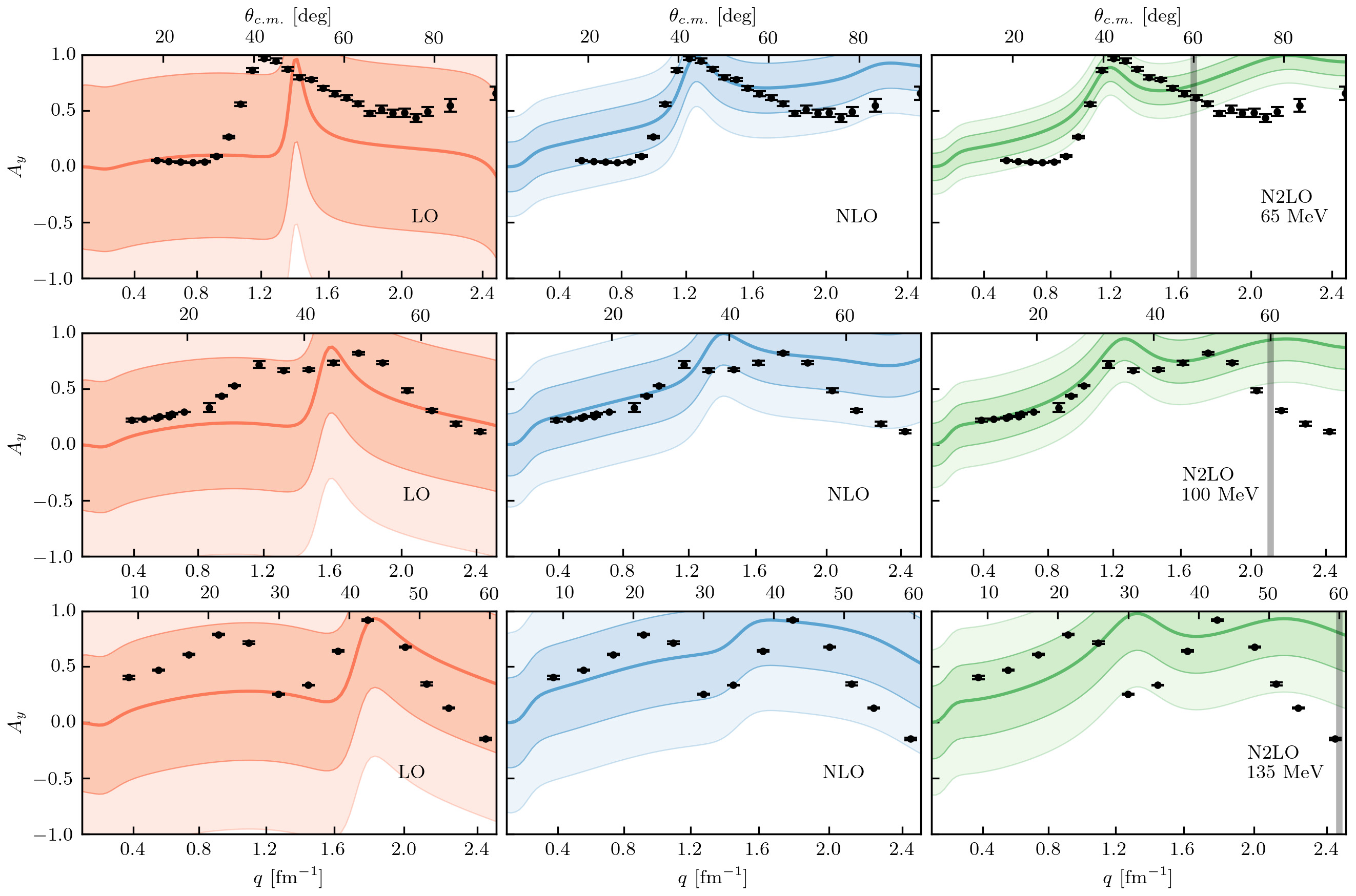
Figure 9: Analyzing power for proton scattering on ¹⁶O at (first row) 65 MeV, (second row) 100 MeV, and (third row) 135 MeV for LO (left column), NLO (middle column), and N2LO (right column) with corresponding $1\sigma$ (darker bands) and $2\sigma$ (lighter bands) error bands. Black dots are experimental data from Refs. Sakaguchi et al. (1979) (65 MeV), Seifert (1990) (100 MeV), and Kelly et al. (1989) (135 MeV). Figure taken from Ref. Baker et al. (2022).

The analyzing powers for proton scattering on ¹⁶O (Fig. 9) are again similar to the ¹²C case. At lower energies (65 and 100 MeV), we again see a good reproduction to within $1\sigma$ or $2\sigma$ of the forward direction data, but beyond $\theta_{\mathrm{c.m.}}=60^{\circ}$, the experimental data is outside the uncertainty bands. At the higher energy of 135 MeV, many of the experimental data are within the uncertainty bands but for a nucleus of this size, the expansion parameter has already increased such that the resulting uncertainty bands are unhelpfully large.

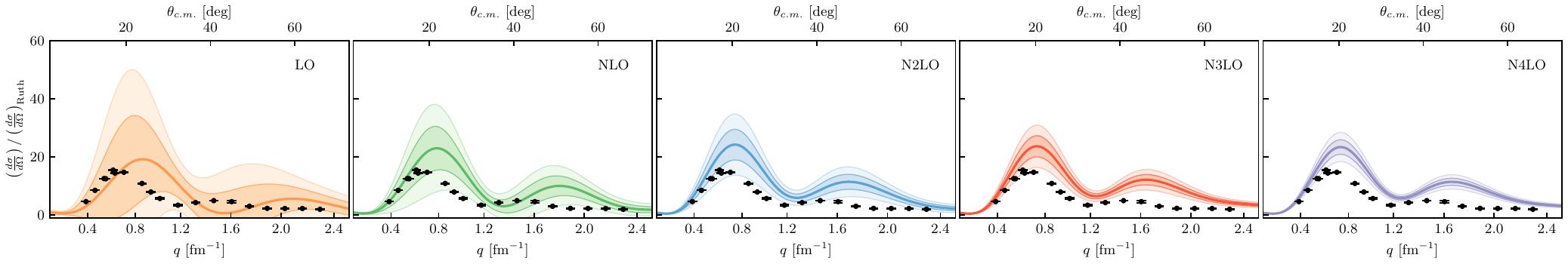
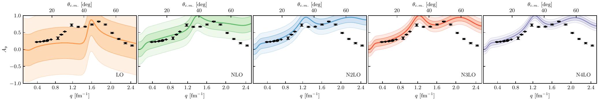
Figure 10: Differential cross section divided by the Rutherford cross section (top) and analyzing power (bottom) for proton scattering from ¹⁶O at 100 MeV. The first 3 columns are the same as the second rows of Figs. 8 and 9. The additional two rightmost panels are inconsistent calculations with use up to N2LO in the structure calculations and up to N3LO (fourth column) or N4LO (fifth column) in the reaction calculation. Due to the inconsistency of the calculation the uncertainty bands are not fully realistic. The data are the same as cited in Figs. 8 and 9.

As stated toward the beginning of the section we omit three-nucleon forces for consistency with the leading-order optical potential which only treats two active nucleons. Those three-nucleon forces already appear at N2LO in the chiral expansion, however, including them consistently in the structure as well as reaction calculation requires going beyond the leading-order optical potential and is beyond the scope of this work. For the sake of investigating truncation errors in the chiral NN force, one may carry out inconsistent calculation in the sense that the structure part of the calculation is kept fixed at N2LO, and in the reaction part higher orders in the NN force are used. Proceeding in this fashion is sensible, since the scattering calculation is more sensitive to the NN force compared to the structure calculation, provided this structure calculation gives a reasonable description of the ground state one-body density. To show how the chiral truncation error develops when higher chiral orders in the NN interaction are introduced, we show in Fig. 10 proton scattering from ¹⁶O at 100 MeV projectile energy, where the higher chiral orders are only employed in the scattering part through the corresponding Wolfenstein amplitudes. In both, the differential cross section as well as the analyzing power the two most right panels depicting the inconsistent calculation show that the uncertainty bands become smaller when higher chiral orders in the NN interaction are included. However, these uncertainty bands are not necessarily realistic due to missing higher-body effects, which include higher orders in the chiral force as well as higher orders in the multiple scattering expansion. Therefore, we can not draw firm conclusions from the fact that data are outside the uncertainty estimates. Nevertheless, it is obvious that the decrease in the uncertainties in the chiral truncation is rather slow due to the large expansion parameter. Furthermore, the medians of the calculations shown in Figs. 8 and 9 do not change when higher chiral orders are considered in Fig. 10, which further indicates that the smaller error bands of the higher order chiral truncations may be artificial.

IV.4 Analysis of Posteriors

Even while restricting our analysis to a region where we expect the expansion parameter to be constant, we can still observe effects on the uncertainty bands if the expansion parameter is large, as noted in many of the results at larger projectile energies. In fact, this behavior will place limits on the size of nucleus that can be considered with this approach, since $p_{NA}$ as defined by Eq. (37) will continue to increase as $A$ increases, yielding $Q>1$ eventually. While this situation is not ideal, we nonetheless find support for it in our analysis after examining the posteriors for $Q$, in accordance with Ref. Baker et al. (2022); Melendez et al. (2019).

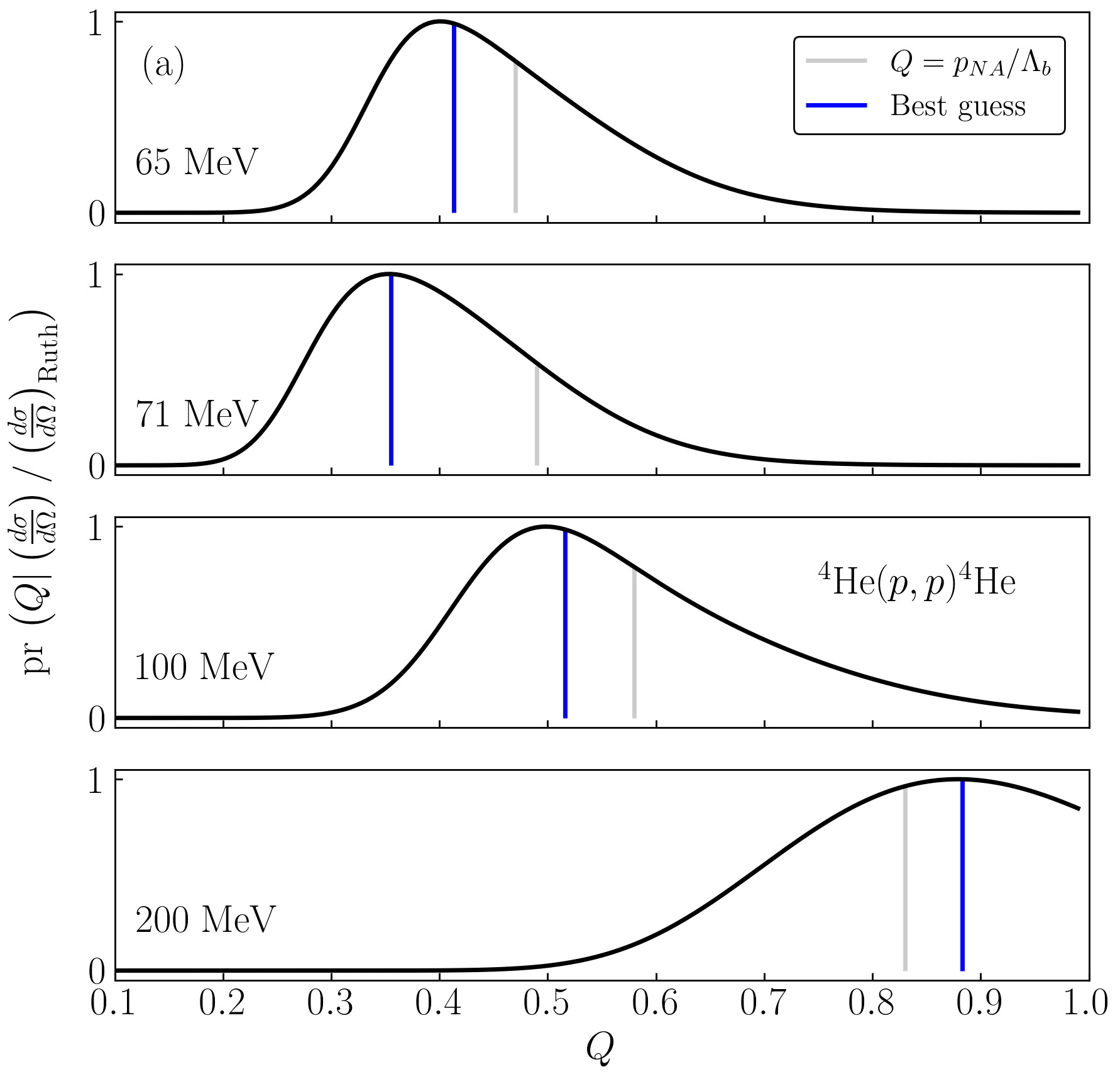
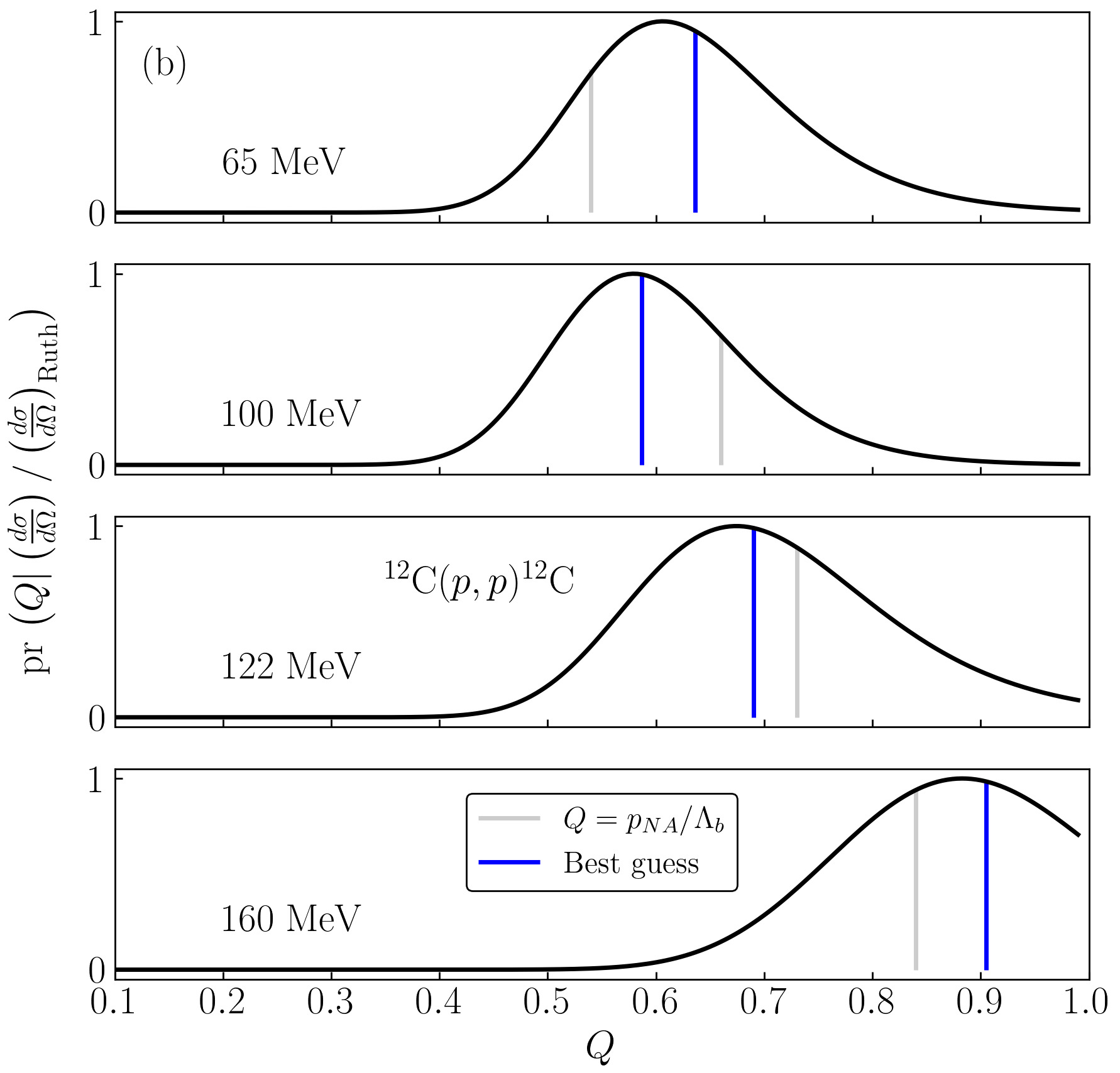
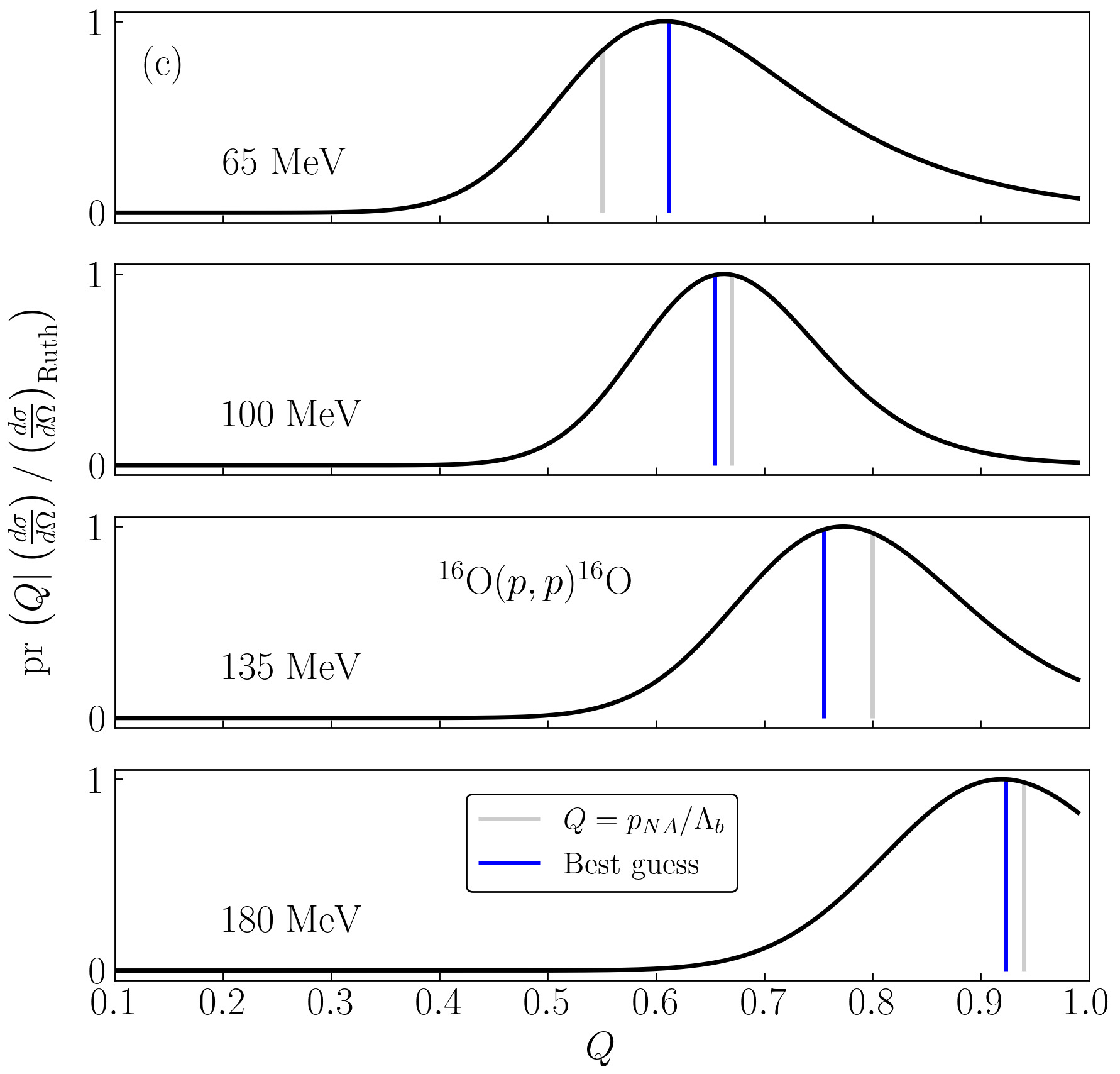
Figure 11: Posterior plots for the expansion parameter $Q$ given the differential cross sections for proton scattering on (a) ⁴He, (b) ¹²C, and (c) ¹⁶O.

In Fig. 11, we calculated posteriors for the differential cross sections in proton scattering from ⁴He, ¹²C, and ¹⁶O at the energies previously discussed. From these, we can extract a single best guess for the value of $Q$ based on the order-by-order calculations and compare that to the expectation for $Q$ based on Eq. (38). For ¹⁶O, the largest nucleus considered, we see generally good agreement between the expected value of $Q$ and the best guess value from the posteriors (Fig.11c). However, as the nucleus decreases in size and as the laboratory energy decreases, some differences begin to emerge between the two values. In Fig. 11b for ¹²C, the comparisons are roughly similar to the ¹⁶O case, but for the ⁴He analysis (Fig. 11a), the differences are more pronounced, especially for the lower laboratory energies. A similar analysis of neutron scattering on ¹²C did not show any significant differences between the two values Baker et al. (2022), which implies ⁴He may be the outlier in this approach. This analysis may imply scattering from ⁴He with projectiles at lower energies could be analyzed with a smaller expansion parameter $Q$, though the higher energy results still favor the larger expansion parameter. As the smallest nucleus considered here, it may also point to the few-body character of ⁴He, which has not historically been well captured in an optical potential approach.

V Outlook

Procedures that quantify the theoretical uncertainties associated with the underlying chiral EFT NN interaction are by now well established for the NN and nucleon-deuteron systems as well as nuclear structure calculations, while the systematic study of chiral truncation uncertainty is not as widely used in ab initio effective interaction employed to describe the scattering of protons or neutrons from nuclei. Contributing factors for this relatively slow development include that when considering a multiple scattering approach to deriving this effective NA interaction in an ab initio fashion only recent progress in calculating the leading-order term in the multiple scattering approach has allowed to treat the NN interaction on the same footing in the structure and reaction part Burrows et al. (2020) by considering the spin of the struck target nucleon. Though calculations showed that the latter does not contribute significantly to observables when considering scattering from nuclei with a $0^{+}$ ground state, one nevertheless needs a consistent ab initio implementation of the leading-order term of the effective NA interaction in order to study the theoretical uncertainties imprinted on NA observables by the chiral EFT NN interaction.

In this work we carry out a systematic study of chiral truncation uncertainties of the EKM chiral interaction on the ab initio effective NA interaction calculated in leading order of the spectator expansion for ⁴He, ¹²C, and ¹⁶O. We find that this interaction allows for a good description of experiment at energies around 100 MeV projectile kinetic energy and slightly lower, provided we focus on regions of momentum transfer where the analysis of the EFT truncation uncertainty is valid. When considering the lower energy of 65 MeV, the agreement with data starts to deteriorate. This is an indication that errors other than the truncation error in the chiral interaction should come into play, specifically errors that result from the spectator expansion itself. Theoretical consideration of the next-to-leading-order term in the spectator expansion are described in some detail in this work in order to lay out necessary theoretical and computational developments for this nontrivial endeavor. At at the next-to-leading order three-nucleon forces will naturally enter the effective interaction. At present this step has only been attempted in approximative fashions, namely by approximating the next-to-leading order in the propagator expansion via a nuclear mean field force Chinn et al. (1995a) or by introducing an effective, density dependent NN potential in the scattering part of the calculation Vorabbi et al. (2021). Since we are not considering next-to-leading order terms in the spectator expansion, we restrict our analysis to N2LO in the chiral interaction and only consider two-nucleon forces. In this case the choice of the EKM interaction with a semi-local coordinate space regulator of 1.0 fm is advantageous Maris et al. (2021), since this specific interaction gives a slightly better description of the ground state energies in the upper $p$-shell compared to other more recent chiral EFT interactions when using two-nucleon interactions only.

In our study the chiral truncation errors at energies larger than 100 MeV increase considerably and the agreement with experiment deteriorates. The increase in the chiral truncation error can simply be traced back to the expansion parameter in our approach is getting too large. The deterioration of the agreement with experiment when going to higher energies is more difficult to answer. One conclusion may be that the specific EKM chiral interaction employed here in using the leading-order in the spectator expansion is not well suited to describe proton-nucleus scattering observables for ⁴He, ¹²C, and ¹⁶O at higher energies. For the chiral NN interaction from Ref. Ekström et al. (2013) this is not the case as shown in Refs. Burrows et al. (2020, 2019). Therefore one will have to investigate what features of a chiral NN interaction are most relevant for a description of NA scattering observables for light nuclei.

To put this in perspective, let us reconsider the basic ideas of the spectator expansion. By design, the leading-order term should be dominant at energies 150 MeV projectile kinetic energy and higher, since the reaction time of the projectile with nucleons inside the nucleus is short, and thus an ‘impulse approximation’ is in general very good. However, we do not want to consider here projectile energies larger than 400 MeV, where a relativistic treatment e.g. via the Dirac equation may be preferred Cooper et al. (1993); Hynes et al. (1985). Thus at energies around 200 MeV the leading order term by design should give a reasonably good description of NA scattering data. This has been the case in the microscopic calculations of the 1990s (see e.g. Crespo et al. (1992, 1990); Elster et al. (1997, 1990); Arellano et al. (1990a, b)) and a set of recent calculations with specific chiral NN interactions Burrows et al. (2019, 2020); Vorabbi et al. (2021). Attempts to go beyond the leading order by incorporating 3NFs in a density dependent fashion into the many-body propagator Vorabbi et al. (2021) indicate that effects at 200 MeV are only visible at higher momentum transfer. In a similar fashion, investigations going beyond the leading order term in Ref. Chinn et al. (1995a) indicate that those effects become important at around 100 MeV and at higher momentum transfers. Thus, if the 3NFs inherent in the chiral expansion are needed to influence calculations with chiral NN forces in the leading order of the spectator expansion at higher energies, then a new look at the interplay between NN and 3NFs in the leading-order spectator expansion must be developed.

Tables

	4He	12C	16O
	Binding energy (MeV)
LO	$45.45(0.01)$	$137.(1.)$	$224.(2.)$
NLO	$28.53(0.01)(3.5)$	$97.(3.)(9.)$	$156.(5.)(14.)$
N2LO	$28.11(0.01)(0.9)$	$94.(4.)(3.)$	$149.(5.)(4.)$
expt	$28.30$	$92.16$	$127.62$
	Point-proton radius (fm)
LO	$1.08(0.02)$	$1.85(0.17)$	$1.8(0.2)$
NLO	$1.40(0.02)(0.08)$	$2.04(0.16)(0.09)$	$2.05(0.16)(0.10)$
N2LO	$1.42(0.02)(0.02)$	$2.12(0.15)(0.03)$	$2.11(0.15)(0.03)$
expt	$1.46$	$2.32$	$2.58$

Table 1: Ground state binding energies (top) and point-proton RMS radii (bottom) of ⁴He, ¹²C, and ¹⁶O with LO, NLO, and N²LO LENPIC SCS NN potentials. Both our estimated numerical uncertainties (first set of uncertainties) and chiral truncation uncertainty estimates (second set of uncertainties, not evaluated for LO) are given.

References

- Bethe (1935) H. A. Bethe, Phys. Rev. 47, 747 (1935).
- Feshbach (1958a) H. Feshbach, Ann. Rev. Nucl. Part. Sci. 8, 49 (1958a).
- Watson (1953) K. M. Watson, Phys. Rev. 89, 575 (1953).
- Francis and Watson (1953) N. C. Francis and K. M. Watson, Phys. Rev. 92, 291 (1953).
- Kerman et al. (1959) A. K. Kerman, H. McManus, and R. M. Thaler, Ann. Phys. 8, 551 (1959).
- Siciliano and Thaler (1977) E. R. Siciliano and R. M. Thaler, Phys. Rev. C16, 1322 (1977).
- Ernst et al. (1977) D. J. Ernst, J. T. Londergan, G. A. Miller, and R. M. Thaler, Phys. Rev. C16, 537 (1977).
- Tandy and Thaler (1980) P. C. Tandy and R. M. Thaler, Phys. Rev. C22, 2321 (1980).
- Crespo et al. (1992) R. Crespo, R. C. Johnson, and J. A. Tostevin, Phys. Rev. C 46, 279 (1992).
- Crespo et al. (1990) R. Crespo, R. C. Johnson, and J. A. Tostevin, Phys. Rev. C 41, 2257 (1990).
- Elster et al. (1997) Ch. Elster, S. P. Weppner, and C. R. Chinn, Phys. Rev. C 56, 2080 (1997).
- Elster et al. (1990) Ch. Elster, T. Cheon, E. F. Redish, and P. C. Tandy, Phys. Rev. C 41, 814 (1990).
- Arellano et al. (1990a) H. F. Arellano, F. A. Brieva, and W. G. Love, Phys. Rev. C 41, 2188 (1990a), [Erratum: Phys. Rev.C 42, 1782 (1990)].
- Arellano et al. (1990b) H. F. Arellano, F. A. Brieva, and W. G. Love, Phys. Rev. C 42, 652 (1990b).
- Entem and Machleidt (2003) D. R. Entem and R. Machleidt, Phys. Rev. C 68, 041001 (2003).
- Epelbaum (2006) E. Epelbaum, Prog. Part. Nucl. Phys. 57, 654 (2006).
- Epelbaum et al. (2009) E. Epelbaum, H.-W. Hammer, and U.-G. Meissner, Rev. Mod. Phys. 81, 1773 (2009), arXiv:0811.1338 [nucl-th] .
- Epelbaum et al. (2015a) E. Epelbaum, H. Krebs, and U. G. Meißner, Phys. Rev. Lett. 115, 122301 (2015a), arXiv:1412.4623 [nucl-th] .
- Epelbaum et al. (2015b) E. Epelbaum, H. Krebs, and U. G. Meißner, Eur. Phys. J. A 51, 53 (2015b), arXiv:1412.0142 [nucl-th] .
- Reinert et al. (2018) P. Reinert, H. Krebs, and E. Epelbaum, Eur. Phys. J. A 54, 86 (2018), arXiv:1711.08821 [nucl-th] .
- Machleidt and Entem (2011) R. Machleidt and D. R. Entem, Phys. Rept. 503, 1 (2011), arXiv:1105.2919 [nucl-th] .
- Entem et al. (2017) D. R. Entem, R. Machleidt, and Y. Nosyk, Phys. Rev. C 96, 024004 (2017), arXiv:1703.05454 [nucl-th] .
- Langr et al. (2019a) D. Langr, T. Dytrych, J. P. Draayer, K. D. Launey, and P. Tvrdik, Comp. Phys. Comm. 244, 442 (2019a).
- Langr et al. (2019b) D. Langr, T. Dytrych, K. D. Launey, and J. P. Draayer, The Int. J. of High Performance Computing Applications 33, 522 (2019b).
- Shao et al. (2018) M. Shao, H. M. Aktulga, C. Yang, E. G. Ng, P. Maris, and J. P. Vary, Comp. Phys. Comm. 222, 1 (2018), arXiv:1609.01689 [nucl-th] .
- Aktulga et al. (2014) H. M. Aktulga, C. Yang, E. G. Ng, P. Maris, and J. P. Vary, Concurrency and Computation: Practice and Experience 26, 2631 (2014).
- Jung et al. (2013) M. Jung, E. H. Wilson, III, W. Choi, J. Shalf, H. M. Aktulga, C. Yang, E. Saule, U. V. Catalyurek, and M. Kandemir, in Proceedings of the International Conference on High Performance Computing, Networking, Storage and Analysis, SC ’13 (ACM, New York, NY, USA, 2013) pp. 75:1–75:11.
- Navratil et al. (2000) P. Navratil, J. P. Vary, and B. R. Barrett, Phys. Rev. Lett. 84, 5728 (2000), arXiv:nucl-th/0004058 [nucl-th] .
- Roth and Navratil (2007) R. Roth and P. Navratil, Phys. Rev. Lett. 99, 092501 (2007), arXiv:0705.4069 [nucl-th] .
- Barrett et al. (2013) B. Barrett, P. Navrátil, and J. Vary, Prog. Part. Nucl. Phys. 69, 131 (2013).
- Binder et al. (2018) S. Binder, A. Calci, E. Epelbaum, R. J. Furnstahl, J. Golak, K. Hebeler, T. Hüther, H. Kamada, H. Krebs, P. Maris, Ulf-G. Meißner, A. Nogga, R. Roth, R. Skibiński, K. Topolnicki, J. P. Vary, K. Vobig, and H. Witała (LENPIC Collaboration), Phys. Rev. C 98, 014002 (2018), arXiv:1802.08584 [nucl-th] .
- Launey et al. (2016) K. D. Launey, T. Dytrych, and J. P. Draayer, Prog. Part. Nucl. Phys. 89, 101 (2016), arXiv:1612.04298 [nucl-th] .
- Dytrych et al. (2020) T. Dytrych, K. D. Launey, J. P. Draayer, D. J. Rowe, J. L. Wood, G. Rosensteel, C. Bahri, D. Langr, and R. B. Baker, Phys. Rev. Lett. 124, 042501 (2020), arXiv:1810.05757 [nucl-th] .
- Furnstahl et al. (2015) R. J. Furnstahl, N. Klco, D. R. Phillips, and S. Wesolowski, Phys. Rev. C 92, 024005 (2015), arXiv:1506.01343 [nucl-th] .
- Melendez et al. (2017) J. A. Melendez, S. Wesolowski, and R. J. Furnstahl, Phys. Rev. C 96, 024003 (2017), arXiv:1704.03308 [nucl-th] .
- Melendez et al. (2019) J. A. Melendez, R. J. Furnstahl, D. R. Phillips, M. T. Pratola, and S. Wesolowski, Phys. Rev. C 100, 044001 (2019), arXiv:1904.10581 [nucl-th] .
- Epelbaum et al. (2020) E. Epelbaum, J. Golak, K. Hebeler, H. Kamada, H. Krebs, Ulf-G. Meißner, A. Nogga, P. Reinert, R. Skibiński, K. Topolnicki, Y. Volkotrub, and H. Witała, Eur. Phys. J. A 56, 92 (2020), arXiv:1907.03608 [nucl-th] .
- Maris et al. (2021) P. Maris, E. Epelbaum, R. J. Furnstahl, J. Golak, K. Hebeler, T. Hüther, H. Kamada, H. Krebs, Ulf-G. Meißner, J. A. Melendez, A. Nogga, P. Reinert, R. Roth, R. Skibiński, V. Soloviov, K. Topolnicki, J. P. Vary, Yu. Volkotrub, H. Witała, and T. Wolfgruber, Phys. Rev. C 103, 054001 (2021), arXiv:2012.12396 [nucl-th] .
- Burrows et al. (2018) M. Burrows, Ch. Elster, G. Popa, K. D. Launey, A. Nogga, and P. Maris, Phys. Rev. C 97, 024325 (2018), arXiv:1711.07080 [nucl-th] .
- Burrows et al. (2019) M. Burrows, Ch. Elster, S. P. Weppner, K. D. Launey, P. Maris, A. Nogga, and G. Popa, Phys. Rev. C 99, 044603 (2019), arXiv:1810.06442 [nucl-th] .
- Burrows et al. (2020) M. Burrows, R. B. Baker, Ch. Elster, S. P. Weppner, K. D. Launey, P. Maris, and G. Popa, Phys. Rev. C 102, 034606 (2020), arXiv:2005.00111 [nucl-th] .
- Baker et al. (2021) R. B. Baker, M. Burrows, Ch. Elster, K. D. Launey, P. Maris, G. Popa, and S. P. Weppner, Phys. Rev. C 103, 054314 (2021), arXiv:2102.01025 [nucl-th] .
- Baker et al. (2022) R. B. Baker, B. McClung, C. Elster, P. Maris, S. P. Weppner, M. Burrows, and G. Popa, Phys. Rev. C 106, 064605 (2022), arXiv:2112.02442 [nucl-th] .
- Gennari et al. (2018) M. Gennari, M. Vorabbi, A. Calci, and P. Navratil, Phys. Rev. C97, 034619 (2018), arXiv:1712.02879 [nucl-th] .
- Vorabbi et al. (2022) M. Vorabbi, M. Gennari, P. Finelli, C. Giusti, P. Navrátil, and R. Machleidt, Phys. Rev. C 105, 014621 (2022), arXiv:2110.05455 [nucl-th] .
- Vorabbi et al. (2021) M. Vorabbi, M. Gennari, P. Finelli, C. Giusti, P. Navrátil, and R. Machleidt, Phys. Rev. C 103, 024604 (2021), arXiv:2010.04792 [nucl-th] .
- Arellano and Blanchon (2022) H. F. Arellano and G. Blanchon, Eur. Phys. J. A 58, 119 (2022), arXiv:2206.09461 [nucl-th] .
- Feshbach (1958b) H. Feshbach, Annals Phys. 5, 357 (1958b).
- Dickhoff and Barbieri (2004) W. H. Dickhoff and C. Barbieri, Prog. Part. Nucl. Phys. 52, 377 (2004), arXiv:nucl-th/0402034 .
- Idini et al. (2019) A. Idini, C. Barbieri, and P. Navrátil, Phys. Rev. Lett. 123, 092501 (2019), arXiv:1903.04581 [nucl-th] .
- Rotureau et al. (2017) J. Rotureau, P. Danielewicz, G. Hagen, F. M. Nunes, and T. Papenbrock, Phys. Rev. C 95, 024315 (2017), arXiv:1611.04554 [nucl-th] .
- Launey et al. (2021) K. D. Launey, A. Mercenne, and T. Dytrych, Ann. Rev. Nucl. Part. Sci. 71, 253 (2021), arXiv:2108.04894 [nucl-th] .
- Hebborn et al. (2022) C. Hebborn et al., arXiv:2210.07293 (2022), arXiv:2210.07293 [nucl-th] .
- Chinn et al. (1995a) C. R. Chinn, C. Elster, R. M. Thaler, and S. P. Weppner, Phys. Rev. C52, 1992 (1995a).
- Chinn et al. (1993a) C. R. Chinn, Ch. Elster, and R. M. Thaler, Phys. Rev. C 47, 2242 (1993a).
- Miller et al. (1978) G. A. Miller, N. Austern, and M. Silver, Phys. Rev. C 17, 835 (1978).
- Chinn et al. (1993b) C. R. Chinn, Ch. Elster, and R. M. Thaler, Phys.Rev. C48, 2956 (1993b).
- Chinn et al. (1995b) C. R. Chinn, C. Elster, R. M. Thaler, and S. P. Weppner, Phys. Rev. C 51, 1418 (1995b).
- Wolfenstein and Ashkin (1952) L. Wolfenstein and J. Ashkin, Phys. Rev. 85, 947 (1952).
- Fachruddin et al. (2000) I. Fachruddin, Ch. Elster, and W. Glöckle, Phys. Rev. C 62, 044002 (2000), arXiv:nucl-th/0004057 [nucl-th] .
- Golak et al. (2010) J. Golak, W. Glöckle, R. Skibinski, H. Witala, D. Rozpedzik, K. Topolnicki, I. Fachruddin, Ch. Elster, and A. Nogga, Phys. Rev. C 81, 034006 (2010), arXiv:1001.1264 [nucl-th] .
- Burrows (2020) M. Burrows, Ab Initio Leading Order Effective Interactions for Scattering of Nucleons from Light Nuclei, Ph.D. thesis, Ohio University (2020).
- Cunningham et al. (2011) E. S. Cunningham, J. S. Al-Khalili, and R. C. Johnson, Phys. Rev. C84, 041601 (2011).
- Cunningham et al. (2013) E. S. Cunningham, J. S. Al-Khalili, and R. C. Johnson, Phys. Rev. C87, 054601 (2013).
- Møller (1945) C. Møller, K. Dan. Vidensk. Sels. Mat. Fys. Medd. 23, 1 (1945).
- Rodberg and Thaler (1967) L. Rodberg and R. Thaler, Introduction of the Quantum Theory of Scattering, Pure and Applied Physics, Vol 26 (Academic Press, 1967).
- Navratil (2004) P. Navratil, Phys. Rev. C70, 014317 (2004).
- Cockrell et al. (2012) C. Cockrell, J. P. Vary, and P. Maris, Phys. Rev. C86, 034325 (2012), arXiv:1201.0724 [nucl-th] .
- Mihaila and Heisenberg (1999) B. Mihaila and J. H. Heisenberg, Phys. Rev. C60, 054303 (1999), arXiv:nucl-th/9802032 [nucl-th] .
- Navratil (2021) P. Navratil, Phys. Rev. C 104, 064322 (2021), arXiv:2109.04017 [nucl-th] .
- Binder et al. (2016) S. Binder, A. Calci, E. Epelbaum, R. J. Furnstahl, J. Golak, K. Hebeler, H. Kamada, H. Krebs, J. Langhammer, S. Liebig, P. Maris, Ulf-G. Meißner, D. Minossi, A. Nogga, H. Potter, R. Roth, R. Skibiński, K. Topolnicki, J. P. Vary, and H. Witała (LENPIC Collaboration), Phys. Rev. C 93, 044002 (2016), arXiv:1505.07218 [nucl-th] .
- Note (1) One commonly applies a Similarity Renormalization Group (SRG) transformation to the NN potential in order to improve the convergence of the many-body calculation. However, this leads to induced three-nucleon forces that are non-negligible; omitting those would lead to a strong dependence on the SRG parameter. We therefore choose to not employ such a transformation here. For the binding energies we use an exponential extrapolation to the complete basis, with associated uncertainties, see Ref. Binder et al. (2016) for details. Radii converge rather slowly in a harmonic oscillator basis, and they do not necessarily converge monotonically with increasing ; furthermore, in the scattering calculations we use densities obtained at fixed values of the harmonic oscillator parameters and . We therefore simply give in Table 1 our results for the point-proton radii of 12C and 16O at , averaged over the range MeV (the same range as is used for the scattering calculations). The numerical uncertainty estimates for the radii listed in Table 1 correspond to the spread over this interval; this is a systematic uncertainty due to the Gaussian fall-off of harmonic oscillator basis functions, and is therefore strongly correlated for the different chiral orders. However, the trend of a significant increase in the radii going from LO to NLO, followed by a smaller increase going from NLO to N2LO, is robust, and correlates with the decrease in binding energies going from LO to NLO to N2LO. Note that we did not include any chiral EFT corrections to the operator; and the experimental point-proton radii are extracted from the charge radius measured in electron scattering experiments, using standard proton and neutron finite-size corrections, relativistic corrections, and meson-exchange corrections.
- Ekström et al. (2013) A. Ekström, G. Baardsen, C. Forssén, G. Hagen, M. Hjorth-Jensen, G. R. Jansen, R. Machleidt, W. Nazarewicz, et al., Phys. Rev. Lett. 110, 192502 (2013).
- Cooper et al. (1993) E. D. Cooper, S. Hama, B. C. Clark, and R. L. Mercer, Phys. Rev. C 47, 297 (1993).
- Hynes et al. (1985) M. V. Hynes, A. Picklesimer, P. C. Tandy, and R. M. Thaler, Phys. Rev. C 31, 1438 (1985).
- Imai et al. (1979) K. Imai, K. Hatanaka, H. Shimizu, N. Tamura, K. Egawa, K. Nisimura, T. Saito, H. Sato, and Y. Wakuta, Nuclear Physics A 325, 397 (1979).
- Burzynski et al. (1989) S. Burzynski, J. Campbell, M. Hammans, R. Henneck, W. B. Lorenzon, et al., Phys.Rev. C 39, 56 (1989).
- Goldstein et al. (1970) N. P. Goldstein, A. Held, and D. G. Stairs, Canadian Journal of Physics 48, 2629 (1970), https://doi.org/10.1139/p70-326 .
- Moss et al. (1980) G. A. Moss et al., Phys. Rev. C 21, 1932 (1980).
- Ieiri et al. (1987a) M. Ieiri, H. Sakaguchi, M. Nakamura, H. Sakamoto, H. Ogawa, M. Yosol, T. Ichihara, N. Isshiki, Y. Takeuchi, H. Togawa, T. Tsutsumi, S. Hirata, T. Nakano, S. Kobayashi, T. Noro, and H. Ikegami, Nuclear Instruments and Methods in Physics Research Section A: Accelerators, Spectrometers, Detectors and Associated Equipment 257, 253 (1987a).
- Kato et al. (1985) S. Kato, K. Okada, M. Kondo, K. Hosono, T. Saito, N. Matsuoka, K. Hatanaka, T. Noro, S. Nagamachi, H. Shimizu, K. Ogino, Y. Kadota, S. Matsuki, and M. Wakai, Phys. Rev. C 31, 1616 (1985).
- Strauch and Titus (1956) K. Strauch and F. Titus, Phys. Rev. 103, 200 (1956).
- Gerstein et al. (1957) G. Gerstein, J. Niederer, and K. Strauch, Phys. Rev. 108, 427 (1957).
- Meyer et al. (1983) H. O. Meyer, P. Schwandt, W. W. Jacobs, and J. R. Hall, Phys. Rev. C 27, 459 (1983).
- Ieiri et al. (1987b) M. Ieiri, H. Sakaguchi, M. Nakamura, H. Sakamoto, H. Ogawa, M. Yosol, T. Ichihara, N. Isshiki, Y. Takeuchi, H. Togawa, T. Tsutsumi, S. Hirata, T. Nakano, S. Kobayashi, T. Noro, and H. Ikegami, Nucl. Instrum. Methods Phys. Res. A 257, 253 (1987b).
- Sakaguchi et al. (1979) H. Sakaguchi, M. Nakamura, K. Hatanaka, A. Goto, T. Noro, F. Ohtani, H. Sakamoto, and S. Kobayashi, Phys. Lett. B 89, 40 (1979).
- Seifert (1990) H. Seifert, Energy Dependence of the Effective Interaction for Nucleon-Nucleus Scattering, Ph.D. thesis, University of Maryland (1990).
- Kelly et al. (1989) J. J. Kelly, W. Bertozzi, T. N. Buti, J. M. Finn, F. W. Hersman, C. Hyde-Wright, M. V. Hynes, M. A. Kovash, B. Murdock, B. E. Norum, B. Pugh, F. N. Rad, A. D. Bacher, G. T. Emery, C. C. Foster, W. P. Jones, D. W. Miller, B. L. Berman, W. G. Love, J. A. Carr, and F. Petrovich, Phys. Rev. C 39, 1222 (1989).
- Kelly et al. (1990) J. J. Kelly, J. M. Finn, W. Bertozzi, T. N. Buti, F. W. Hersman, C. Hyde-Wright, M. V. Hynes, M. A. Kovash, B. Murdock, P. Ulmer, A. D. Bacher, G. T. Emery, C. C. Foster, W. P. Jones, D. W. Miller, and B. L. Berman, Phys. Rev. C 41, 2504 (1990).