ODIM: an efficient method to detect outliers via inlier-memorization effect of deep generative models

Abstract

Identifying whether a given sample is an outlier or not is an important issue in various real-world domains. This study aims to solve the unsupervised outlier detection problem where training data contain outliers, but any label information about inliers and outliers is not given. We propose a powerful and efficient learning framework to identify outliers in a training data set using deep neural networks. We start with a new observation called the inlier-memorization (IM) effect. When we train a deep generative model with data contaminated with outliers, the model first memorizes inliers before outliers. Exploiting this finding, we develop a new method called the outlier detection via the IM effect (ODIM). The ODIM only requires a few updates; thus, it is computationally efficient, tens of times faster than other deep-learning-based algorithms. Also, the ODIM filters out outliers successfully, regardless of the types of data, such as tabular, image, and sequential. We empirically demonstrate the superiority and efficiency of the ODIM by analyzing 20 data sets.

1 Introduction

Outlier (also anomaly) is an observation that differs significantly from other observations, and outlier detection (OD) is the task of identifying outliers in a given data set. OD has wide applications such as fraud detection, fault detection, and defect detection in images. OD is also used as a pre-processing step in supervised learning to filter out anomalous training samples, which may degrade the performance of a predictive model.

OD problems can be categorized into three areas in general: 1) Supervised outlier detection (SOD) requires label information about whether each training sample is inlier (also normal) or outlier and solves the two-class classification task. A limitation of SOD is that it is hard to access the entirely labeled data set in practice. 2) Semi-supervised outlier detection (SSOD) refers to methods that assume all training data being inliers and construct patterns or models for the inliers. SSOD can be interpreted as the one-class classification task since information of outliers is not used during the training procedure. Similarly to SOD, it is not common to have a data set composed of only inliers (Chandola et al., 2009; Chalapathy & Chawla, 2019). 3) Unsupervised outlier detection (UOD) deals with the most realistic situations where training data include some outliers but no label information about anomalousness is available. Most anomaly detection tasks in practice are related to UOD since the information of outliers in massive data is hardly known in advance.

In this study, we propose a novel algorithm for UOD problems. Our algorithm is motivated by so called the memorization effect observed in noisy label problems (Arpit et al., 2017; Jiang et al., 2018). The goal of noisy label problems is to learn an accurate classifier when some of the class labels in the training data are contaminated. When standard supervised learning algorithms are applied to such mislabeled data, an interesting phenomenon so called the memorization effect is observed where correctly labeled data are learned earlier and mislabeled data are learned later in the training phase of deep neural networks. The memorization effect makes it possible to detect mislabeled data by comparing per-sample losses in an early stage of the training phase. The aim of this paper is to apply the memorization effect to UOD problems to develop a novel algorithm for detecting outliers with high accuracy as well as high efficiency in computation.

There already exists a study utilizing the memorization effect for UOD problems. (Wang et al., 2019a) noticed that during a deep discriminative model is trained via the self-supervised learning framework, the model memorizes inliers first and outliers next in the training phase, and named this phenomenon the inlier-priority effect. Generating more than a hundred artificial classes with a pre-specified annotation strategy, they suggested a method, called $E^{3}$-Outlier, which identifies outliers with high accuracy.

Even though it works effectively, but $E^{3}$-Outlier is specialized to image data and not easy to be extended for other domains of data such as tabular data, sequential data as well as special image data including wafer images generated from semiconductor fabrications. This is because $E^{3}$-Outlier annotates the training data using a method that is specialized for image data.

As a domain-agnostic UOD solver which can be used as an off-the-shelf method, we develop a new method that inherits the idea of the memorization effect but does not require any prior expertise in data. We start with finding a new and interesting observation that the memorization effect is also observed in learning a deep generative model. That is, when we train a deep generative model with training data that includes outliers, the inliers’ loss values reduce prior to those of outliers at early updates. We call this observation the inlier-memorization (IM) effect. The IM effect occurs because, in the early training phase, decreasing the loss values of inliers rather than outliers is a more beneficial direction to reduce the overall loss function. Detailed discussions about the IM effect are given in Section 3.2 and 3.3. Note that deep generative models does not require class labels, thus domain-specific techniques such as the annotation method used in $E^{3}$-Outlier are not necessary and so our method is domain-agnostic.

Utilizing the IM effect, we propose a simple but powerful OD solver called the outlier detection via the IM effect (ODIM) to identify outliers from a given training data set. We train a deep generative model with a log-likelihood-based approach such as the VAE (Kingma & Welling, 2013) or IWAE (Burda et al., 2016) for a few updates, and we regard data with large loss values compared to the per-sample loss distribution as outliers.

As the IM effect is sensitive to how many updates of a deep generative model proceed, the key to the success of our method is to choose the optimal number of updates to utilize the IM effect maximally. For this purpose, we develop the following strategy. At each update, we fit the Gaussian mixture model with two components to the per-sample loss distribution and evaluate the Wasserstein distance of the two components. We chase the distance as the update proceeds and select the optimal update point at which the distance becomes the largest.

Our method has several advantages over existing OD methods. First, as mentioned above, the ODIM is agnostic to data domains such as tabular, sequential or image since it is built on unsupervised learning. By analyzing numerous data sets, 20 in total, rooted in various domains, we demonstrate that the ODIM consistently yields competitive or superior results in identifying outliers. See Section 4.

Second, the ODIM is efficient in computational time and resources because it requires only a few training updates, usually a few epochs, in the training phase to detect outliers. Thus, even when we train multiple generative models to utilize an ensemble technique, the ODIM is still much faster than other recent UOD solvers such as (Ruff et al., 2018b; Lai et al., 2020a) which require at least 200 training epochs.

Third, the ODIM is relatively insensitive to the choice of the hyper-parameters; thus, it is easy to apply to real problems without much effort. In contrast, most existing UOD methods have the objective functions with regularized terms that should be controlled carefully (Ruff et al., 2018b, 2020; Lai et al., 2020b). For example, they are even sensitive to the choice of the learning scheduler. Sensitivity to the hyper-parameters makes it difficult to use the corresponding algorithms in practice.

This paper is organized as follows. Section 2 provides a brief review for related researches for OD problems. The detailed descriptions of the ODIM algorithm with discussions of the IM effect are given in Section 3. Results of various experiments including performance tests and ablation studies are presented in Section 4. Further discussions are provided in Section 5 and concluding remarks follow in Section 6.

The key contributions of this work are:

• We find a new phenomenon called the IM effect that deep generative models memorize inliers prior to outliers at early training phases.

• We develop a simple and domain-agnostic UOD learning method called the ODIM to identify outliers in a given unlabeled training data set contaminated with anomalous samples.

• We empirically demonstrate the superiority and efficiency of our method by analyzing various benchmark data sets.

2 Related works

In this section, we only consider SSOD and UOD problems.

Semi-supervised outlier detection

A popular technique for SSOD is the one class classification approach which transforms data into a feature space and distinguishes outliers from inliers by their radii from the center on the feature space. The OCSVM (Schölkopf et al., 2001) and SVDD (Tax & Duin, 2004) are two representative algorithms, which use kernel techniques to construct the feature space.

Succeeding their ideas, plenty of SSOD algorithms using deep neural networks have been developed. The DeepSVDD (Ruff et al., 2018a) extends the SVDD by utilizing a deep autoencoder (AE) for learning a feature map, and the DeepSAD (Ruff et al., 2020) modifies the DeepSVDD to incorporate labeled outliers to training data. Modifications of the DeepSVDD have been developed by (Zong et al., 2018; Mahmood et al., 2021; Xia et al., 2015). In addition to AE, deep generative models are also popularly used for SSOD (Ryu et al., 2018; Nalisnick et al., 2019; Jiang et al., 2022). There are methods for SSOD other than the one class classification approach. The SimCLR (Chen et al., 2020) and BERT (Devlin et al., 2019) utilize self-supervised learning by generating artificial labels automatically to obtain a desirable feature map, and various algorithms based on this idea have been developed (Golan & El-Yaniv, 2018a; Bergman & Hoshen, 2020; Tack et al., 2020; Sehwag et al., 2021). When some labels (not related to inliers or outliers) are available, feature maps for classification of those labels can be used for distinguishing outliers from inliers (Hendrycks & Gimpel, 2017; Liang et al., 2018; Gomes et al., 2022).

Unsupervised outlier detection

As for traditional approaches, the LOF (Breunig et al., 2000a) compares the density of a given datum compared to the densities of its neighborhoods, and the IF (Liu et al., 2008a) utilizes the fact that outliers can be separated out by random trees with relatively small sizes. The UOCL (Liu et al., 2014) solves UOD problems by employing pseudo soft labels and training them jointly with the one-class classification model.

There are various methods to solve UOD problems with deep learning models. The RDA (Zhou & Paffenroth, 2017) combines the robust PCA and AE to detect outliers. The DSEBM (Zhai et al., 2016) utilizes the energy-based model for density estimation and uses the energy score or reconstruction error to identify outliers. The RSRAE (Lai et al., 2020b) devises a new hidden layer called RSR, inserting it between encoder and decoder of a deep AE to separate inliers and outliers effectively. The $E^{3}$-Outlier (Wang et al., 2019a) trains a deep neural network by self-supervised learning and identifies outliers based on how fast the loss decreases as the training proceeds.

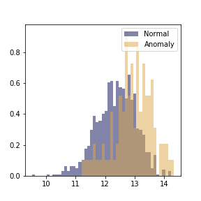
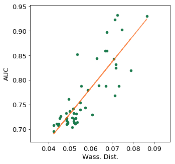
Figure 1: (Left) The Euclidean norm distribution of Cardio data. There is no significant distributional discrepancy between inliers and outliers. (Middle) The distribution of the per-sample loss values of Cardio data after training a single epoch. A significant gap between the distributions of inliers and outliers is seen. (Right) The positive relationship between the Wasserstein distance and identifying performance (AUC) on Cardio data.

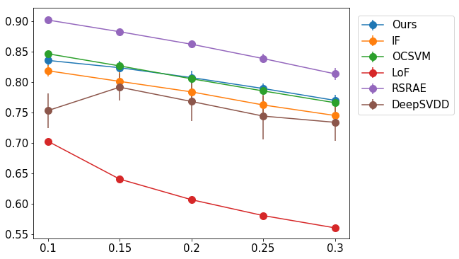
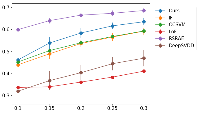
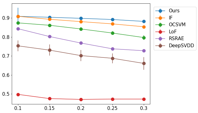
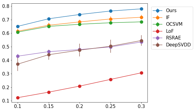
Figure 2: Comparison results of (Left) AUC and (Right) AP values varying the pollution rate $r$ from 0.1 to 0.3. We analyze two data sets: (Upper) MNIST and (Lower) FMNIST. Vertical bars present the standard deviations.

3 Proposed method

3.1 Notations and definitions

For a given input vector ${\bf x}\in\mathbb{R}^{D}$, we denote its anomalousness by $y^{o}\in\{0,1\}$, that is, $y^{o}=0$ if ${\bf x}$ is an inlier and $y^{o}=1$ otherwise. Note that only ${\bf x}$ is observable but $y^{o}$ is not under the UOD task. Let $\mathcal{U}^{tr}=\{{\bf x}_{1},\ldots,{\bf x}_{n}\}$ be unlabeled training data. Our goal is to detect outlier samples, i.e. ${\bf x}$ with $y^{o}=1$, from $\mathcal{U}^{tr}$ as accurately as possible. Let $p({\bf x}|{\bf z};\theta)$ and $q({\bf z}|{\bf x};\phi)$ be given encoder and decoder parameterized by $\theta$ and $\phi$, respectively, where ${\bf z}\in\mathbb{R}^{d}$ (generally assuming $d<D$) is a latent vector.

For a given $p\in\mathbb{N}$, we denote the $l_{p}$-norm of a vector $\mathbf{a}$ by $\|\mathbf{a}\|_{p}$. For two real-valued functions defined on $\mathbb{R}^{+}$, $f(t)$ and $g(t)$, $f(t)$ is said to be $\Theta(g(t))$ if there exist positive constants $C_{1},C_{2}$ and $T$ such that $C_{1}\cdot g(t)\leq f(t)\leq C_{2}\cdot g(t)$ holds for all $t\geq T$.

3.2 Main motivation: inlier-memorization effect

Before proposing our method, we first explain the main motivation - the inlier-memorization effect. Suppose that we are training a deep generative model with a certain learning framework where the training data contain both inliers and outliers. For an illustration of the IM effect, we analyze Cardio data set and train a deep generative model using the VAE method (Kingma & Welling, 2013). The encoder and decoder architectures are 2-layered deep neural networks (DNNs) with $d=5$ and 50 hidden nodes for each hidden layer. We are to closely look at the per-sample loss distribution in an early training phase. For this purpose, we train the encoder and decoder by minimizing the VAE loss function only for one epoch.

The middle panel in Figure 1 shows the empirical distribution of the per-sample loss values of the training data. We can observe that the loss values of inliers tend to be smaller than those of outliers, which means that the generative model is trained in the direction of memorizing inliers first at the beginning of the training phase, and we call this phenomenon the inlier-memorization (IM) effect.

Conceptually, the IM effect is not a surprising phenomenon. Assume that the per-sample loss function is continuous on the input space. Hence, reducing the loss function on dense regions of the input space is beneficial to reduce the overall loss function (e.g. the negative log-likelihood). Since inliers usually locate on dense regions while outliers locate on sparse regions, reasonable learning algorithms would focus more on dense regions in an early stage of the training phase, which results in the IM effect. Note that the IM effect is observed only in an early training phase since the learned model memorizes both of inliers and outliers in a later training phase.

Remark 3.1.

The IM effect is associated with so-called the memorization effect in the noisy label problem. When we train a deep classification model with training data that contains some samples whose labels are contaminated, the model tends to memorize cleanly labeled data before noisily labeled ones in the early training phase (Arpit et al., 2017; Jiang et al., 2018). This phenomenon can be understood similarly to the intuition of the IM effect: the data with clean labels are distributed more densely than noise ones. And because of noisy data are surrounded by clean ones, reducing a noisy sample’s loss even harms the losses of many clean data close to the noisy one, leading to a clear discrepancy of contribution to the overall loss reduction for clean data and noise data.

3.3 Theoretical analysis

We provide a theoretical explanation of the inlier-memorization effect with a toy example where we train a linear factor model using the VAE. That is, $p({\bf x}|{\bf z};\theta)$ is the density function of $W{\bf z}+b+\epsilon$, where $W\in\mathbb{R}^{D\times d},b\in\mathbb{R}^{D}$ are the loading matrix and bias vector and $\epsilon\sim N(0_{D},\sigma^{2}I_{D})$ is a noise vector. For $q,$ we set $q({\bf z}|{\bf x};\phi)$ as the density function of $U{\bf x}+v+\tau$, where $U\in\mathbb{R}^{d\times D}$, $U\in\mathbb{R}^{d}$, and $\tau\sim{\cal N}(0_{d},\eta^{2}I_{d})$. Here, we set $\sigma$ and $\eta$ as fixed values. Thus, $\theta$ and $\phi$ are $(W,b)$ and $(U,v)$, respectively. Note that the objective function of the VAE for a given input vector ${\bf x}$ is given as

$$L^{\text{VAE}}(\theta,\phi;{\bf x}):=\mathbb{E}_{{\bf z}\sim q({\bf z}|{\bf x};\phi)}\left[\log\left(\frac{p({\bf x}|{\bf z};\theta)p({\bf z})}{q({\bf z}|{\bf x};\phi)}\right)\right],$$ (1)

where $p({\bf z})$ is the density function of the standard multivariate Gaussian distribution. We assume that each element in $W,b,U,$ and $v$ is randomly initialized by the i.i.d. uniform distribution on $[-1,1]$. Then we have the following proposition whose proof is given in Appendix.

Proposition 3.2.

For a given input vector ${\bf x}$, the following holds:

$$\begin{split}\mathbb{E}_{\theta,\phi}\left\|\frac{\partial}{\partial\theta}L^{\text{VAE}}(\theta,\phi;{\bf x})\right\|_{2}^{2}=\Theta\left(\|{\bf x}\|_{2}^{4}\right).\end{split}$$

Proposition 1 implies that at the beginning of learning, the Euclidean norm of the gradient of the VAE depends on the euclidean norm of the input vector. It implies that if the norms of inliers and outliers are similar, the initial update direction of $\theta$ is influenced more by inliers than outliers due to their imbalanced proportions. Therefore, in the early training phase, the generative model is trained in the direction of memorizing inliers before outliers and thus the IM effect emerges.

Even though Proposition 1 considers a linear generated model, its implication is still valid for a deep generated model. To confirm this statement, we conduct a simple experiment to support our theoretical explanation of the IM effect by analyzing Cardio data set, already explained in Section 3.2. We normalize the input features of Cardio data so that each feature is ranged between 0 and 1.

Using these normalized data, we train a deep generative model by minimizing the VAE objective function for a single epoch, and take a look at the per-sample loss distributions of inliers and outliers. The result is given in the middle panel of Figure 1 where the per-sample losses of the inliers are much smaller than those for the outliers. This IM effect can be explained as follows. The similarity of the distributions of the norms of inliers and outliers is shown in the left panel of Figure 1 and Proposition 1 implies that the norm of the per-sample gradient is similar for inliers and outliers and thus the initial update direction of $\theta$ is determined mainly by the inliers (because the number of inliers is much larger) to yield the IM effect.

3.4 Outlier detection via inlier-memorization effect: Algorithm

The IM effect provides a way of detecting outlier by utilizing the per-sample loss values of a deep generative model at an early training phase. In this subsection, we propose a new learning algorithm for solving UOD problems, which is called the outlier detection via the inlier-memorization effect (ODIM). The ODIM algorithm consists of two steps: 1) train a deep generative model for a pre-specified number of updates and 2) based on the per-sample loss values, regard a given sample as an outlier when the corresponding loss value is large. To implement this idea, a couple of additional techniques are needed which are explained below.

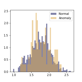
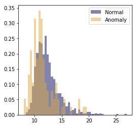
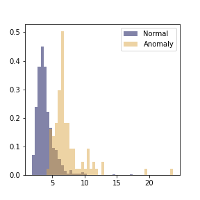
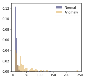
Figure 3: Distributions of per-sample (Left) data norms and (Right) gradient norms on Cardio. We consider two pre-processing schemes to normalize each feature: 1) (Upper) min-max pre-processing, and 2) (Lower) standardization pre-processing.

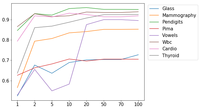
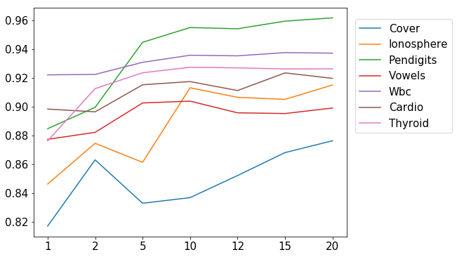
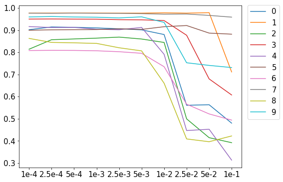
Figure 4: (Left) AUC results on tabular data sets with various number of samples drawn from $q({\bf z}|{\bf x};\phi)$. (Middle) AUC results on tabular data sets with various number of models from one to twenty to take ensemble. (Right) AUC results on FMNIST for each class with various learning rates. We vary the learning rate from 1e-4 to 1e-1.

Algorithm 1 ODIM
In practice, we set $(K,N_{\text{u}},N_{\text{pat}})=(50,10,10)$.

Input: Training data set $\mathcal{U}^{tr}=\{{\bf x}_{1},...,{\bf x}_{n}\}$

0:  : Decoder: $p({\bf x}|{\bf z};\eta)$, Encoder: $q({\bf z}|{\bf x};\phi)$, GMM-2: $\pi_{1}\mathcal{N}(\mu_{1},\sigma_{1}^{2})+\pi_{2}\mathcal{N}(\mu_{2},\sigma_{2}^{2})$, Mini-batch size: $n_{\text{mb}}$, Optimizer: $\mathcal{O}$, Number of samples in IWAE: $K$, Update unit number: $N_{\text{u}}$, Maximum patience: $N_{\text{pat}}$

0:  : Auto-encoder: $p({\bf x}|{\bf z};\eta)$ and $q({\bf z}|{\bf x};\phi)$, Classifier: $f(\mathbf{x};\theta)$, GMM-2: $\pi_{1}\mathcal{N}(\mu_{1},\sigma_{1}^{2})+\pi_{2}\mathcal{N}(\mu_{2},\sigma_{2}^{2})$

  while $n_{\text{pat}}<N_{\text{pat}}$ do

     for k in $1:N_{\text{u}}$ do

        1. Generate a subset $U$ with the mini-batch size of $n_{\text{mb}}$ from $\mathcal{U}^{tr}$.

        2. Using the mini-batch $U$ and optimizer $\mathcal{O}$, update $\theta$ and $\phi$ with the mini-batch version of (4).

        $l_{i}\leftarrow\widehat{L}^{\text{IWAE}}({\bf x}_{i};\theta,\phi)$ for $i=1,\ldots,n$.// per-sample loss

        $\{\tilde{l}_{i}\}_{i=1}^{n}$ $\leftarrow$ $normalize(\{{l}_{i}\}_{i=1}^{n})$. // normalize loss values

        Fit the parameters in GMM-2 using $\{\tilde{l}_{i}\}_{i=1}^{n}$.

        if $d_{\text{WD}}>D_{\text{WD}}^{\text{max}}$ then

           $D_{\text{WD}}^{\text{max}}$ $\leftarrow$ $d_{\text{WD}}$ // update the maximum Wasserstein distance

           $l_{i}^{*}$ $\leftarrow$ $l_{i}$, $i=1,\ldots,n$ // update the best inlier scores

           $\theta^{*},\phi^{*}$ $\leftarrow$ $\theta,\phi$ // save the best parameters

           $n_{\text{pat}}$ $\leftarrow$ $0$

        else

           $n_{\text{pat}}$ $\leftarrow$ $n_{\text{pat}}+1$

        end if

     end for

  end whileOutput: $l_{i}^{*},i=1,\ldots,n$ // best inlier scores Output: $\theta^{*},\phi^{*}$ // best parameters

Table 1: Description of tabular data sets

Data	Size	# features	# outliers (%)	Data	Size	# features	# outliers (%)
BreastW	683	9	239 (35%)	Vowels	1456	12	50 (3.4%)
Cover	286048	10	2747 (0.9%)	Wbc	278	30	21 (5.6%)
Glass	214	9	9 (4.2%)	Arrhythmia	452	274	66 (15%)
Ionosphere	351	33	126 (36%)	Cardio	1831	21	176 (9.6%)
Mammography	11183	6	260 (2.32%)	Satellite	6435	36	2036 (32%)
Musk	3062	166	97 (3.2%)	Satimage-2	5803	36	71 (1.2%)
Pendigits	6870	16	156 (2.27%)	Shuttle	49097	9	3511 (7%)
Pima	768	8	268 (35%)	Thyroid	3772	6	93 (2.5%)

Table 2: Training AUC value comparisons on tabular data sets

Data	IF	OCSVM	LOF	DeepSVDD	RSRAE	Ours
BreastW	0.983	0.817	0.447	0.863	0.507	0.992
Cover	0.894	0.914	0.553	0.522	0.820	0.837
Glass	0.714	0.265	0.802	0.815	0.480	0.725
Ionosphere	0.859	0.758	0.894	0.827	0.969	0.914
Mammography	0.862	0.846	0.754	0.696	0.535	0.848
Musk	0.999	0.816	0.370	0.759	0.726	1.000
Pendigits	0.957	0.936	0.486	0.613	0.907	0.953
Pima	0.672	0.626	0.648	0.027	0.587	0.706
Vowels	0.807	0.607	0.946	0.787	0.876	0.904
Wbc	0.938	0.934	0.937	0.763	0.598	0.941
Arrhythmia	0.810	0.807	0.786	0.677	0.814	0.800
Cardio	0.931	0.913	0.716	0.589	0.245	0.916
Satellite	0.690	0.598	0.558	0.637	0.731	0.690
Satimage-2	0.992	0.979	0.491	0.739	0.988	0.997
Shuttle	0.997	0.983	0.508	0.646	0.972	0.981
Thyroid	0.977	0.847	0.942	0.781	0.815	0.928

Table 3: Training AP value comparisons on tabular data sets

Data	IF	OCSVM	LOF	DeepSVDD	RSRAE	Ours
BreastW	0.961	0.843	0.308	0.678	0.392	0.988
Cover	0.049	0.085	0.012	0.012	0.149	0.032
Glass	0.080	0.032	0.170	0.149	0.104	0.119
Ionosphere	0.821	0.730	0.850	0.757	0.951	0.867
Mammography	0.211	0.108	0.103	0.053	0.024	0.098
Musk	0.999	0.124	0.025	0.132	0.057	1.000
Pendigits	0.291	0.211	0.038	0.039	0.215	0.302
Pima	0.507	0.456	0.446	0.431	0.427	0.491
Vowels	0.149	0.085	0.442	0.124	0.227	0.375
Wbc	0.560	0.553	0.557	0.206	0.113	0.710
Arrhythmia	0.448	0.415	0.394	0.362	0.518	0.443
Cardio	0.536	0.543	0.195	0.140	0.059	0.564
Satellite	0.673	0.583	0.389	0.461	0.688	0.652
Satimage-2	0.902	0.847	0.027	0.031	0.887	0.949
Shuttle	0.980	0.951	0.084	0.167	0.713	0.947
Thyroid	0.541	0.148	0.239	0.124	0.186	0.327

Table 4: Averaged ranks of AUC and AP over tabular data sets

	IF	OCSVM	LOF	DeepSVDD	RSRAE	Ours
AUC	2.094	3.813	4.250	4.750	4.000	2.094
AP	2.313	3.813	4.250	4.813	3.688	2.125

Table 5: Results of AUC and AP over the WM-811K data set. We write the standard deviations of each method inside the parentheses.

	IF	OCSVM	LOF	DeepSVDD	RSRAE	Ours
AUC	0.680 (0.004)	0.731	0.327	0.505 (0.114)	0.672 (0.011)	0.747 (0.005)
AP	0.354 (0.008)	0.418	0.072	0.151 (0.063)	0.203 (0.019)	0.379 (0.003)

Table 6: Results of AUC and AP over the Reuters-21578 data set. We write the standard deviations of each method inside the parentheses.

	IF	OCSVM	LOF	DeepSVDD	RSRAE	Ours
AUC	0.574 (0.063)	0.878	0.812	0.501 (0.033)	0.915 (0.022)	0.888 (0.043)
AP	0.202 (0.051)	0.536	0.388	0.130 (0.022)	0.610 (0.063)	0.553 (0.096)

Table 7: Running time comparison for the ODIM and other competitors. All records are measured in seconds.

Data	IF	OCSVM	LOF	DeepSVDD	RSRAE	Ours
Cover	6.192	2164.270	24.959	3463.820	2451.950	358.378
Mammography	0.408	2.482	0.221	135.958	98.356	21.002
Pendigits	0.350	1.246	1.899	83.944	62.739	15.998
Satellite	0.369	1.152	1.735	78.876	71.493	13.846
Satimage-2	0.361	0.916	1.340	72.048	69.147	8.580
Shuttle	0.987	63.146	4.426	594.588	427.291	61.471
FMNIST	4.298	52.114	15.446	744.652	1495.926	32.859
Wafer	89.499	11498.385	910.600	4561.028	12363.401	149.986
Reuters	4.984	106.567	1.394	16.567	23.931	92.486

Table 8: Test AUC results of the ODIM. For MNIST, FMNIST, and Reuters, we set $r=0.1$.

Data	IF	OCSVM	LOF	Ours
BreastW	0.986	0.880	0.458	0.994
Cover	0.876	0.915	0.554	0.852
Glass	0.563	0.680	0.720	0.725
Ionosphere	0.850	0.736	0.890	0.861
Mammography	0.613	0.485	0.848	0.861
Musk	0.869	0.840	0.720	1.000
Pendigits	0.999	0.821	0.318	0.946
Pima	0.650	0.527	0.557	0.714
Vowels	0.960	0.948	0.418	0.870
Wbc	0.691	0.651	0.638	0.936
Arrhythmia	0.493	0.515	0.547	0.817
Cardio	0.348	0.435	0.482	0.919
Satellite	0.747	0.458	0.957	0.692
Satimage-2	0.924	0.900	0.914	0.995
Shuttle	0.824	0.756	0.664	0.985
Thyroid	0.926	0.922	0.711	0.921
MNIST	0.825	0.857	0.693	0.843
FMNIST	0.899	0.873	0.496	0.905
Wafer	0.683	0.732	0.329	0.723
Reuters	0.484	0.918	0.829	0.859

Table 9: Test AP results of the ODIM. For MNIST, FMNIST, and Reuters, we set $r=0.1$.

Data	IF	OCSVM	LOF	Ours
BreastW	0.968	0.890	0.311	0.988
Cover	0.056	0.095	0.013	0.034
Glass	0.140	0.122	0.213	0.152
Ionosphere	0.803	0.729	0.857	0.815
Mammography	0.261	0.109	0.066	0.106
Musk	0.997	0.126	0.024	1.000
Pendigits	0.300	0.241	0.028	0.295
Pima	0.537	0.517	0.478	0.539
Vowels	0.120	0.058	0.517	0.266
Wbc	0.605	0.332	0.353	0.549
Arrhythmia	0.490	0.324	0.281	0.403
Cardio	0.583	0.525	0.207	0.612
Satellite	0.679	0.593	0.376	0.659
Satimage-2	0.925	0.872	0.029	0.959
Shuttle	0.951	0.950	0.061	0.837
Thyroid	0.587	0.065	0.068	0.392
MNIST	0.974	0.978	0.954	0.976
FMNIST	0.984	0.982	0.905	0.987
Wafer	0.423	0.496	0.109	0.451
Reuters	0.782	0.971	0.933	0.923

Table 10: Comparison of two data pre-processing methods: 1) min-max and 2) standardization. We report the AUC results.

Data	Min-max	Standardization
BreastW	0.992	0.664
Cover	0.837	0.961
Glass	0.725	0.630
Ionosphere	0.914	0.863
Mammography	0.848	0.767
Musk	1.000	0.799
Pendigits	0.953	0.941
Pima	0.706	0.437
Vowels	0.904	0.639
Wbc	0.941	0.856
Arrhythmia	0.800	0.769
Cardio	0.916	0.943
Satellite	0.690	0.740
Satimage-2	0.997	0.969
Shuttle	0.981	0.995
Thyroid	0.928	0.965

Table 11: Training AUC values with various values of $l$. We consider three values for $l$, $l=0.0,0.3,0.5$.

Data	$l=0.0$	$l=0.3$	$l=0.5$
Arrhythmia	0.800	0.837	0.888
Cardio	0.916	0.991	0.993
Satellite	0.690	0.868	0.881
Satimage-2	0.997	0.998	0.999
Shuttle	0.981	0.990	0.990
Thyroid	0.928	0.995	0.995

Table 12: Training AP values with various values of $l$. We consider three values for $l$, $l=0.0,0.3,0.5$.

Data	$l=0.0$	$l=0.3$	$l=0.5$
Arrhythmia	0.443	0.767	0.772
Cardio	0.564	0.934	0.943
Satellite	0.652	0.849	0.849
Satimage-2	0.949	0.954	0.958
Shuttle	0.947	0.977	0.979
Thyroid	0.327	0.844	0.845

Choice of the learning algorithm for a deep generative model

We should choose a learning algorithm for a deep generative model carefully to make the IM effect appear more clearly. There exist numerous algorithms to train a deep generative model, which can be roughly divided into two approaches: 1) maximizing the log-likelihood (Kingma & Welling, 2013; Burda et al., 2016; Rezende & Mohamed, 2015; Tomczak & Welling, 2018; Kim et al., 2020) and 2) using adversarial networks (Goodfellow et al., 2014; Nowozin et al., 2016; Arjovsky et al., 2017; Gulrajani et al., 2017).

It is well-known that adversarial-network-based methods provide more realistic data. But due to their inherent feature of searching the saddle points (i.e. solving the min-max problem), it is difficult to define the per-sample loss and thus it is not suitable for the ODIM.

In contrast, the per-sample loss in the likelihood approach is naturally defined as the per-sample negative log-likelihood value, and thus it is easy to develop the ODIM algorithm with the log-likelihood-based approach. Calculation of the likelihood function, however, is computationally difficult. To resolve this problem, we use a computable lower bound of the log-likelihood, such as the evidence lower bound (ELBO) used in the variational autoencoder (VAE, (Kingma & Welling, 2013)).

There exist several lower bounds on the log-likelihood tighter than ELBO (Burda et al., 2016; Tomczak & Welling, 2018; Kim et al., 2020). Among them, we decide to employ the importance weighted autoencoder (IWAE, (Burda et al., 2016)) because IWAE can control the tightness of its lower bound to the log-likelihood and is relatively easy to compute. Usually, the IM effect becomes more obvious when the lower bound is tighter, but more computation is required to make the lower bound be tighter.

The objective function of the IWAE is given as:

$$\begin{split}{L}^{\text{IWAE}}&(\theta,\phi;{\bf x})\\ :=&\mathbb{E}_{{\bf z}_{1},...,{\bf z}_{K}\sim q({\bf z}|{\bf x};\phi)}\left[\log\left(\frac{1}{K}\sum_{k=1}^{K}\frac{p({\bf x}|{\bf z}_{k};\theta)p({\bf z}_{k})}{q({\bf z}_{k}|{\bf x};\phi)}\right)\right],\end{split}$$ (2)

where $p({\bf z})$ is the density of the standard multivariate Gaussian distribution and $K$ is the number of samples. Note that the IWAE reduces to the VAE when $K=1$. In practice, the IWAE utilizes the Monte Carlo method to approximate (2) by

$$\widehat{L}^{\text{IWAE}}(\theta,\phi;{\bf x}):=\log\left(\frac{1}{K}\sum_{k=1}^{K}\frac{p({\bf x},{\bf z};\theta)p({\bf z}_{k})}{q({\bf z}_{k}|{\bf x};\phi)}\right),$$ (3)

where ${\bf z}_{k},k=1,\ldots,K$ are independently drawn from $q({\bf z}|{\bf x};\phi)$. We train the encoder and decoder simultaneously by maximizing the empirical expectation of (3)

$$\mathbb{E}_{{\bf x}\sim{\cal U}^{tr}}\left[\widehat{L}^{\text{IWAE}}(\theta,\phi;{\bf x})\right]=\frac{1}{n}\sum_{i=1}^{n}\widehat{L}^{\text{IWAE}}(\theta,\phi;{\bf x}_{i}),$$ (4)

with respect to $\theta$ and $\phi$ simultaneously over ${\cal U}^{tr}.$

It is known that ${L}^{\text{IWAE}}(\theta,\phi;{\bf x})$ converges to the log-likelihood as $K$ goes to infinity (Burda et al., 2016). However, a larger $K$ requires more computation and hence we need to choose $K$ carefully to compromise performance and computation. In this study, we set the value of $K$ to 50. An ablation study for the role of $K$ is done whose results are given in Section 4.4.

Choice of the optimal number of updates

We empirically find out that the IM effect usually appears at very early in the training phase, even sometimes fewer than a single epoch, and the degree of the IM effect (i.e., the difference of the loss distributions between inliers and outliers) depends sensitively on the number of updates of the model. Moreover, the optimal number of updates varies from data to data. Thus, it would be a key for the success of the ODIM algorithm to choose the optimal number of updates data adaptively.

We devise a heuristic strategy to decide the number of updates where the IM effect is maximized. At each update of the model, we assess the degree of bimodality of the per-sample loss distribution and select the optimal number of updates at which the degree of bimodality is maximized. To be more specific, let $l_{1},\ldots,l_{n}$ be $n$ be the normalized loss values calculated with the current estimated generative model, having values between 0 and 1, of the training data. We fit the two component Gaussian mixture model (GMM-2) ${\pi}_{1}\mathcal{N}({\mu}_{1},{\sigma}_{1}^{2})+{\pi}_{2}\mathcal{N}({\mu}_{2},{\sigma}_{2}^{2})$ on these loss values, and then we investigate how much the two normal distributions in the fitted Gaussian mixture model are different to measure the degree of bimodality. For the discrepancy measure of two normal distributions, we use the Wasserstein distance which is given as

$$W_{2}(\mathcal{N}({\mu}_{1},{\sigma}_{1}^{2}),\mathcal{N}({\mu}_{2},{\sigma}_{2}^{2}))=({\mu}_{1}-{\mu}_{2})^{2}+({\sigma}_{1}-{\sigma}_{2})^{2}.$$ (5)

The right panel in Figure 1 illustrates the values of AUC on the training data of Cardio at the first $10\times m$ updates for $m=1,\ldots,50$ and their corresponding Wasserstein distances. We can clearly see that the Wasserstein distance is a useful measure for selecting the optimal number of updates.

In practice, we calculate the Wasserstein distance at every $N_{\text{u}}$ update and terminate the update when the largest Wasserstein distance has not been improved for $N_{\text{pat}}$ many calculations of the Wasserstein distance in a row, and select the optimal number of updates as the one at which the Wasserstein distance is maximized. We set $N_{\text{u}}$ and $N_{\text{pat}}$ to 10 in all the following numerical experiments unless specifically stated.

We summarize the ODIM’s pseudo algorithm in Algorithm 1.

Ensemble of ODIM scores

To improve and stabilize our method, we adopt an ensemble strategy. We train multiple models to have multiple best models for detecting outliers. From the best models, we obtain multiple per-sample loss values for each datum, and take the average of them to yield the final score. The number of multiple models is fixed to 10 in our experiments. We will empirically show the effectiveness of using multiple models in Section 4.4.

Since the IM effect is maximized at early in the training phase and learning multiple models can be done in parallel, the ensemble ODIM is still faster than other deep learning algorithms which require hundreds of training epochs.

4 Numerical experiments

In this section, we show the superiority of our proposed method empirically through extensive experiments. We analyze numerous data sets, 20 in total, that cover tabular, image, and sequential types. We show that the performance of the ODIM for detecting outliers is favorably compared with other competitors regardless of data types. We also carry out ablation studies including the running time analysis and effect of hyper-parameters.

In the experiments, we report the averaged results based on five trainings with randomly initialized parameters. We apply the Pytorch framework to implement our algorithm using a single NVIDIA TITAN XP GPU. We leave our implementation code on our GitHub web page.

4.1 Data set description

Tabular data sets

We consider 16 tabular data sets which are frequently analyzed in the OD literature. They are obtained from various domains, such as clinical pathology or astronomy, and are publicly accessible on (Rayana, 2016). We refer Table 1 for the detailed descriptions of the data sets. All the data sets have the labels about the anomalous information, but we exclude them in the training phase to conduct unsupervised learning tasks, but use them in the test phase to assess the accuracy of outlier detection.

MNIST & Fashion MNIST

We analyze two synthetic image data sets made from MNIST (LeCun et al., 1998) and FMNIST (Xiao et al., 2017). MNIST and FMNIST contain grey-colored $28\times 28$ images of handwritten digits and clothing, respectively. Both data sets consist of 60K training data and 10K test data.

To conduct UOD tasks, we pre-process the two data sets in advance, as is done in the previous works (Ruff et al., 2018b; Chalapathy et al., 2018; Golan & El-Yaniv, 2018b; Wang et al., 2019b). We choose a class $c$ to be the normal class and regard the others as abnormal classes. We select all the training images whose class is $c$ and randomly draw samples from the remaining data so that the ratio between the number of inlier and outlier data is $1:r$, where $r\in[0,1]$ is a pre-specified pollution rate. Then, we combine the normal and abnormal data and discard their class labels to make unlabeled data. Note that both MNIST and FMNIST have ten classes; thus, we can generate ten types of training data with the pollution rate $r.$ We report averaged performance on the ten training data unless otherwise stated.

WM-811K

We also investigate the real-world image data set, WM-811K (Wu et al., 2014), containing wafer images obtained from the semiconductor fabrication process. Among 811K images, we pick a part of images with label information about whether a given image is a failure (outlier). As a result, we utilize 172,950 wafers that include 25,519 failure images. Since the data have diverse sizes, we resize them to have the unified shape of $28\times 28$ before analyzing them.

Reuters-21578

Besides tabular and image data, we additionally analyze text type data. Reuters-21578 data set is a collection of 21,578 documents from Reuters newswire in 1987. We follow the procedure in (Lai et al., 2020a) to make analyzable data. We use the pre-processed data with a fixed dimension of 26,147 by applying the TFIDF transformer. We consider the five largest classes among 90 classes and randomly draw 360 samples randomly from each class. Similar to MNIST and FMNIST, we build training data using a pre-specified pollution rate $r$ for each class and report averaged results over the five classes.

4.2 Implementation details

Data pre-process

In addition to identifying outliers in a given training data set, we also assess the identification performance in unseen (test) data. We use the given test data for MNIST and FMNIST. For the other data sets, we randomly split each data set into two partitions with the rate of 6:4 and use the first and second partitions as training and test data sets, respectively.

After the training and test data are constructed, we apply the min-max normalization to them so that each feature has the minimum zero and maximum one. We mainly focus on the detecting performance on training data, and present the performance on test data in Section 4.4 of ablation study.

Architecture & learning schedule

We use two hidden layered DNN architectures for building the encoder and decoder and set $K$, the number of samples drawn from the encoder used for constructing the IWAE objective function, to 50. We optimize the IWAE loss function with the Adam optimizer (Kingma & Ba, 2014) with the mini-batch size of 128 and the learning rate of 5e-4. To run the ODIM, we fix the two hyper-parameters, $N_{\text{u}}$ and $N_{\text{pat}}$, to 10. For the ensemble learning, we train 10 pairs of encoder and decoder, each of which is trained from different initialized parameter values. See our GitHub web page for the detailed implementations.

Baseline

For baselines to be compared with the ODIM, we consider three machine-learning-based methods: 1) isolation forests (IF, (Liu et al., 2008b)), 2) one-class SVM (OCSVM, (Schölkopf et al., 2001)), and 3) local outlier factor (LOF, (Breunig et al., 2000b)), and two deep-learning-based methods: 4) deep support vector data description (DeepSVDD, (Ruff et al., 2018b)) and 5) robust subspace recovery autoencoder (RSRAE, (Lai et al., 2020a)).

As for the LOF, OCSVM, and IF methods, we implement them using the scikit-learn package, and we refer to the official GitHub websites of the DeepSVDD and RSRAE for their re-implementations. Like the ODIM, we report their average results on five runs with different initials.

4.3 Performance for outlier identification

We first compare the ODIM with the other baselines in terms of the performance for identifying outliers in a given training data set. We evaluate the two performance scores: the area under receiver operating characteristic (AUC or ROAUC) and average precision (AP).

Results for tabular data

Tables 2 and 3 list the AUC and AP results on the tabular data sets (We mark the best score for each data set as the bold face.). The results amply show the superiority of the ODIM compared to other baselines in identifying outliers since the ODIM achieves the best scores most frequently on both AUC and AP (6 for each). For example, on BreastW and Musk, the ODIM separates inliers and outliers (almost) perfectly.

In addition, it is notable that the AP values of the ODIM are not much different from the best scores when it is not the best, while the AP values of the others have large variations. In particular, the two deep learning based methods, DeepSVDD and RSRAE, show relatively unstable results. For example, the AP values of RSRAE for BreastW and Cardio are much smaller than those of the ODIM.

To check further the stability of the performance for detecting outliers according to the data sets, we rank the AUC and AP scores of the algorithms for each data set and take the average of the ranks for each algorithm to obtain the averaged rank, which is summarized in Table 4. The ODIM achieves the best averaged ranks on both AUC and AP. These stability results imply that the ODIM can be used as an off-the-shelf method for outlier identification of tabular data. In the subsequent analyses, we demonstrate that the ODIM is still stable when dealing with other types of data sets.

MNIST & FMNIST results

Figures 2 compare the results for MNIST and FMNIST data sets. Similar to the tabular data, the ODIM works quite well for image data. Our method achieves the second best performances for all considering pollution rates on MNIST and the best performances on FMNIST.

WM-811K results

We analyze an image data set called WM-811K consisting of various wafer images. Table 5 shows that our method marks the best and the second-best results on AUC and AP, respectively. In contrast, the two deep-learning-based methods do not work well.

Reuters-21578 results

We analyze Reuters to check the efficiency of our method on super-high-dimensional data analysis, whose results are summarized in Table 6. The ODIM records the second-best AUC and AP values succeeding the RSRAE. Meanwhile, the IF, which is compared favorably to the ODIM for tabular data, shows sub-optimal performances.

Conclusion

Throughout the empirical experiments, we have noticed that among the various methods for outlier identification, the ODIM is the only one that performs consistently well regardless of data types.

4.4 Ablation study

Number of samples used in the IWAE

Recall that the IWAE objective function uses multiple samples, ${\bf z}_{1},\ldots,{\bf z}_{K}$, independently drawn from $q({\bf z}|{\bf x};\phi)$, to achieve a tighter lower bound of the log-likelihood. We empirically check that using a tighter bound actually yields a clearer IM effect.

The left panel in Figure 4 summarizes the AUC values on several tabular data sets with various $K$s from 1 to 100. For the results of the other tabular data sets, see Appendix. Note that the IWAE with $K=1$ equals the original VAE. As expected, a lower bound closer to the log-likelihood tends to provide more obvious IM effect, leading to better identification performances. We can also observe that when the value of $K$ becomes larger than 50, the enhancement seems saturated. For this reason, we set $K=50$ in our experiments.

Implementation time

We investigate how fast our method is executed compared to other competitors. Table 7 summarizes the running time comparisons on several data sets, including tabular and image data. As for our method, we only display the running time of a single model learning since training multiple models to make an ensemble can be done in parallel. The results for the other data sets are listed in Appendix.

As expected, the two deep learning methods are much slower than the non-deep-learning-based anomaly detection methods. Our method is generally faster than the deep learning methods. In particular, our method is 45 and 82 times faster than the RSRAE on FMNIST, and Wafer, respectively. This is surprising because our method identifies outliers better than the RSRAE on these data sets. When analyzing data with large sample sizes such as Cover, FMNIST, and Wafer, our method is similar or even faster than non-deep-learning methods.

Our method has relatively inferior performance in running time on Reuters. Unlike the other data sets, Reuters is a super high-dimensional data set with more than 26,000 features. We conjecture that the high dimensionality of data might put off the occurrence of the IM effect. Accelerating the IM effect to overcome the running time issue when analyzing super high-dimensional data should be done, which we will do in a near future.

Number of models to ensemble

We investigate the effect of the ensemble in the ODIM. We vary the number of models used in the ensemble from one to twenty and compare the performances on several tabular data sets, whose results are presented in the middle panel of Figure 4. The results for the other data sets are summarized in Appendix.

There is a general tendency that using more models helps improve the identifying performance. The optimal number of models varies according to data sets, but the performance is not sensitive to the number of models used in the ensemble unless it is too small.

Learning schedule

We evaluate the robustness of the ODIM to the learning schedule. We consider the Adam optimizer with various learning rates from 1e-4 to 1e-1, whose results on FMNIST are depicted in the right panel of Figure 4. We present the results of the ten classes separately, where each class is regarded as the inlier class. Note that the identifying performances rarely change until we use a learning rate larger than 1e-2. As we usually do not consider a learning rate much larger than 1e-3 when we apply the Adam optimizer, we can conclude that our method is stable with respect to the learning schedule, which implies that our method can be used in practice without delicate settings.

Identifying unseen data

As we mentioned in Section 4.2, we have left some portion of data to examine outlier identification ability for unseen data. Table 8 and 9 summarize the test AUC and AP results. On tabular data sets, the results for unseen data are similar to those for training data, indicating that our method identifies normal samples well from unseen data.

Interestingly, the test AP results for the other complex data sets, image and sequential data sets, tend to be higher than those for training data sets regardless of learning methods. We think that for such data the distributions of outliers for training and test data sets are quite different compared to the those of inliers due to their high dimensionality, which results in larger loss values for test outliers to make detecting them easier.

5 Further discussion

5.1 Effect of data pre-processing on the ODIM

Proposition 1 indicates that the gradient norm is proportional to the input norm. An interesting fact is that the input norm is not invariant to the normalization process, and so is the IM effect. This seemingly counter-intuitive phenomenon can be explained as follows. Since the initial parameters in the model considered in Proposition 1 are independent mean 0 random variables, data far from the origin are not explained well by an initial linear factor model, and thus, the norms of the corresponding gradients become larger.

The above observation provides an important implication regarding the IM effect. The IM effect depends on the choice of the normalization process. For illustration, we apply the ODIM to the standardization scaling - a normalization process to force every feature to have mean zero and variance one. Figure 3 compares the input norms and gradient norms of the initial model of the min-max scaled data and the standardization scaled data. It is observed that the input norms of inliers in the min-max scaled data are similar to those of outliers while the input norms of inliers in the standardization scaled data are smaller. In turn, as implied by Proposition 1, the gradient norms of inliers are similar to those of outliers for the min-max scaled data while the gradient norms of outliers are much larger for the standardization scaled data. Note that inliers in the standardization scaled data mostly locate around the origin and thus the input norms of inliers become smaller.

Smaller gradients of inliers generally result in the performance degradation. In Table 10, we empirically observe that among 16 tabular data sets, the ODIM with the standardization scaled data has better results only on five data sets.

Even though it is better than the standardization scaling, the min-max scaling is by no means optimal for the IM effect. We leave the optimal choice of the normalization process and/or choice of initial parameters as a future research topic.

5.2 ODIM with labeled data

When outlier labels are available, some studies have exploited this additional information to solve outlier detection tasks more efficiently (Ruff et al., 2020; Daniel et al., 2019). But as far as we know, these existing works require that all outliers should be labeled, which is equivalent to the SOD setting. The only difference of (Ruff et al., 2020; Daniel et al., 2019) compared to the conventional SOD solvers is that they cast the problem into an one-class classification problem rather than a two-class one.

While it is very costly to obtain perfectly labeled data, partially labeled data are frequently met in practice. In this subsection, we modify the ODIM for such a situation. That means, apart from the unlabeled training data set ${\cal U}^{tr}=\{{\bf x}_{1},\ldots,{\bf x}_{n}\}$, we also have a labeled outlier data set ${\cal L}^{tr}=\{({\bf x}_{1}^{l},1),\ldots,({\bf x}_{m}^{l},1)\}$. Note that there exist outliers in ${\cal U}^{tr}.$

We simply adopt the idea of (Daniel et al., 2019), which encourages the log-likelihood of known outliers to decrease with the variational upper bound. For $u>1$, the upper bound, called $\chi$ upper bound (CUBO), is given as:

$$\begin{aligned} L^{\text{CUBO}}&(\theta,\phi;{\bf x})\\ :=&\frac{1}{u}\log\mathbb{E}_{{\bf z}\sim q({\bf z}|{\bf x};\phi)}\left[\left(\frac{p({\bf x}|{\bf z};\theta)p({\bf z})}{q({\bf z}|{\bf x};\phi)}\right)^{u}\right].\end{aligned}$$ (6)

With the above CUBO term (6), we modify the loss function of the ODIM by subtracting the expected CUBO on ${\cal L}^{tr}$ from the original IWAE loss function to have:

$$\mathbb{E}_{{\bf x}\sim{\cal U}^{tr}}\widehat{L}^{\text{IWAE}}(\theta,\phi;{\bf x})-\gamma\cdot\mathbb{E}_{{\bf x}\sim{\cal L}^{tr}}\widehat{L}^{\text{CUBO}}(\theta,\phi;{\bf x}),$$

where

$$\widehat{L}^{\text{CUBO}}(\theta,\phi;{\bf x}):=\left(\frac{p({\bf x}|{\bf z};\theta)p({\bf z})}{q({\bf z}|{\bf x};\phi)}\right)^{u},$$

for ${\bf z}$ being a random sample drawn from $q({\bf z}|{\bf x};\phi)$ and $\gamma>0$ is a tuning parameter controlling the degree of the CUBO loss. The CUBO loss generally increases the IWAE per-sample loss values of outliers, leading to separating out the two components of the GMM-2 more clearly. In our paper, we set the value of $\gamma$ to one.

To investigate the improvements of our modified method, we assess the training AUC and AP values over several tabular data sets with various proportions of labeled outliers, which are summarized in Table 11 and 12. Here, $l\in[0,1]$ means the ratio of the labeled and entire outliers. Note that the case of $l=0.0$ is equivalent to when we only use ${\cal U}^{tr}$. It is clearly seen that using label information helps to enhance identifying performance with a large margin, especially for the AP, even when the proportion of the labeled data is small.

Note that the proposed modification of the ODIM for partially labeled data can be improved further. For example, we can use the labeled information to select the optimal number of updates. There would be other rooms to improve the ODIM for partially labeled data, which we leave for future works.

6 Concluding remarks

This paper proposed a fast, powerful and easy to use UOD method called the ODIM. The ODIM is inspired by a new observation called the IM effect that deep generative models tend to memorize inliers first when they are trained. Combined with the technique to select the optimal number of training updates and the ensemble method, we found that the ODIM identified outliers effectively and efficiently; the ODIM provided consistently superior results regardless of data types with much faster running times.

As far as the authors know, there are not many theoretical studies about the behavior of deep neural networks at the early training phase. It would be valuable to understand theoretically when and why the IM effect (or the memorization effect) emerges. Based on theoretical understandings, the suboptimal behavior of the ODIM on super high dimensional data could be improved.

Proof of Proposition 1

Note that the objective function of the VAE is given as:

$$L^{\text{VAE}}(\theta,\phi;{\bf x}):=\int_{\bf z}\log\left(\frac{p({\bf x}|{\bf z};\theta)p({\bf z})}{q({\bf z}|{\bf x};\phi)}\right)\cdot q({\bf z}|{\bf x};\phi)d{\bf z}.$$

Thus, we have the equations:

$$\frac{\partial}{\partial w_{ij}}L^{\text{VAE}}(\theta,\phi;{\bf x})=\int_{\bf z}\frac{\partial}{\partial w_{ij}}\log\left(p({\bf x}|{\bf z};\theta)\right)\cdot q({\bf z}|{\bf x};\phi)d{\bf z},$$

and

$$\frac{\partial}{\partial b_{i}}L^{\text{VAE}}(\theta,\phi;{\bf x})=\int_{\bf z}\frac{\partial}{\partial b_{i}}\log\left(p({\bf x}|{\bf z};\theta)\right)\cdot q({\bf z}|{\bf x};\phi)d{\bf z},$$

where $w_{ij}$ and $b_{i}$ for $i\in[D]$ and $j\in[d]$ are the $(i,j)$ element of $W$ and the $i$-th element of $b$, respectively. Here, we define $[L]:=\{1,\ldots,L\}$ for $L\in\mathbb{N}$. Note that

$$\mathbb{E}_{\theta,\phi}\left\|\frac{\partial}{\partial\theta}L^{\text{VAE}}(\theta,\phi;{\bf x})\right\|_{2}^{2} = \sum_{i}\sum_{j}\mathbb{E}_{\theta,\phi}\left[\frac{\partial}{\partial w_{ij}}L^{\text{VAE}}(\theta,\phi;{\bf x})\right]^{2}$$

$$+\sum_{i}\mathbb{E}_{\theta,\phi}\left[\frac{\partial}{\partial b_{i}}L^{\text{VAE}}(\theta,\phi;{\bf x})\right]^{2}.$$

We are going to characterize the two terms, $\mathbb{E}_{\theta,\phi}\left[\frac{\partial}{\partial w_{ij}}L^{\text{VAE}}(\theta,\phi;{\bf x})\right]^{2}$ and $\mathbb{E}_{\theta,\phi}\left[\frac{\partial}{\partial b_{i}}L^{\text{VAE}}(\theta,\phi;{\bf x})\right]^{2}$, and combine them to draw the final conclusion.

w.r.t. $w_{ij}$

Since $X|(Z={\bf z})\sim\mathcal{N}\left(W{\bf z}+b,\sigma^{2}\right)$ holds, we have

$$\log p({\bf x}|{\bf z};\theta) = -\frac{1}{2\sigma^{2}}\sum_{i=1}^{D}\left(x_{i}-{\bf w}_{i}^{\prime}{\bf z}-b_{i}\right)^{2}+const$$

$$= -\frac{1}{2\sigma^{2}}\sum_{i=1}^{D}\left(x_{i}-\sum_{j=1}^{d}w_{ij}z_{j}-b_{i}\right)^{2}+const,$$

where ${\bf w}_{i}$ is the $i$-th row of $W$ and $const$ is a constant not depending on $\theta$. Therefore, we can obtain the following result of the log-likelihood with respect to $w_{ij}$:

$$\frac{\partial}{\partial w_{ij}}\log\left(p({\bf x}|{\bf z};\theta)\right)$$

$$=\frac{1}{\sigma^{2}}\left(x_{i}-{\bf w}_{i}^{\prime}{\bf z}-b_{i}\right)\cdot z_{j}$$

$$=\frac{1}{\sigma^{2}}\left[x_{i}z_{j}-w_{ij}z_{j}^{2}-\sum_{j^{\prime}\neq j}w_{ij^{\prime}}z_{j}z_{j^{\prime}}-b_{i}z_{j}\right].$$

Hence, the first derivative of the VAE objective function with respect to $w_{ij}$ becomes:

$$\frac{\partial}{\partial w_{ij}}L^{\text{VAE}}(\theta,\phi;{\bf x})$$

$$=\int_{\bf z}\frac{1}{\sigma^{2}}\left[(x_{i}-b_{i})z_{j}-w_{ij}z_{j}^{2}-\sum_{j^{\prime}\neq j}w_{ij^{\prime}}z_{j}z_{j^{\prime}}-b_{i}z_{j}\right]\cdot q({\bf z}|{\bf x};\phi)d{\bf z}$$

$$=\frac{1}{\sigma^{2}}\left[(x_{i}-b_{i})({\bf u}_{j}^{\prime}{\bf x}+v_{j})-w_{ij}\left(\left({\bf u}_{j}^{\prime}{\bf x}+v_{j}\right)^{2}+\eta^{2}\right)\right.$$

$$\left.-\left({\bf u}_{j}^{\prime}{\bf x}+v_{j}\right)\sum_{j^{\prime}\neq j}w_{ij^{\prime}}\left({\bf u}_{j^{\prime}}^{\prime}{\bf x}+v_{j^{\prime}}\right)\right]$$

$$=\frac{1}{\sigma^{2}}\left[(x_{i}-b_{i})({\bf u}_{j}^{\prime}{\bf x}+v_{j})\right.$$

$$\left.-\left({\bf u}_{j}^{\prime}{\bf x}+v_{j}\right)\sum_{j^{\prime}}w_{ij^{\prime}}\left({\bf u}_{j^{\prime}}^{\prime}{\bf x}+v_{j^{\prime}}\right)-w_{ij}\eta^{2}\right],$$

where ${\bf u}_{j}$ is the $j$-th row of $U$. By squaring the above term, we have

$$\left[\frac{\partial}{\partial w_{ij}}L^{\text{VAE}}(\theta,\phi;{\bf x})\right]^{2}$$

$$=\frac{1}{\sigma^{4}}\left[{(x_{i}-b_{i})^{2}\left({\bf u}_{j}^{\prime}{\bf x}+v_{j}\right)^{2}}\right.$$

$$\left.+\left({\bf u}_{j}^{\prime}{\bf x}+v_{j}\right)^{2}{\sum_{j^{\prime}}w_{ij^{\prime}}^{2}\left({\bf u}_{j^{\prime}}^{\prime}{\bf x}+v_{j^{\prime}}\right)^{2}}+w_{ij}^{4}\eta^{4}\right.$$

$$+2\left({\bf u}_{j}^{\prime}{\bf x}+v_{j}\right)^{2}\sum_{j^{{}^{\prime\prime}}>j^{\prime}}w_{ij^{\prime}}w_{ij^{\prime\prime}}({\bf u}_{j^{\prime}}^{\prime}{\bf x}+v_{j^{\prime}})({\bf u}_{j^{\prime\prime}}^{\prime}{\bf x}+v_{j^{\prime\prime}})$$

$$+2w_{ij}\eta^{2}\left({\bf u}_{j}^{\prime}{\bf x}+v_{j}\right)\sum_{j^{\prime}}w_{ij^{\prime}}\left({\bf u}_{j^{\prime}}^{\prime}{\bf x}+v_{j^{\prime}}\right)$$

$$-2w_{ij}\eta^{2}(x_{i}-b_{i})\left({\bf u}_{j}^{\prime}{\bf x}+v_{j}\right)$$

$$\left.-2(x_{i}-b_{i})\left({\bf u}_{j}^{\prime}{\bf x}+v_{j}\right)^{2}\sum_{j^{\prime}}w_{ij^{\prime}}\left({\bf u}_{j^{\prime}}^{\prime}{\bf x}+v_{j^{\prime}}\right)\right].$$

Now, we will calculate the expected value of the above equation with respect to $\theta$ and $\phi$. To do this, we are going to take an expectation for each term in the RHS of the above equation. Note that, for a random variable $X\sim Unif[-1,1]$, $\mathbb{E}\left[X\right]=0$, $\mathbb{E}\left[X^{2}\right]=1/3$, and $\mathbb{E}\left[X^{4}\right]=1/5$. Thus, we have

$$\mathbb{E}_{\theta,\phi}\left[(x_{i}-b_{i})^{2}\left({\bf u}_{j}^{\prime}{\bf x}+v_{j}\right)^{2}\right]$$

$$=\mathbb{E}_{\theta,\phi}\left[(x_{i}^{2}-2x_{i}b_{i}+b_{i}^{2})\left(({\bf u}_{j}^{\prime}{\bf x})^{2}+v_{j}^{2}+2v_{j}{\bf u}_{j}^{\prime}{\bf x}\right)\right]$$

$$=\mathbb{E}_{\theta,\phi}\left[(x_{i}^{2}+b_{i}^{2})\left(\sum_{i^{\prime}}u_{ji^{\prime}}^{2}x_{i^{\prime}}^{2}+v_{j}^{2}\right)\right]$$

$$=\left(x_{i}^{2}+\frac{1}{3}\right)\cdot\left(\frac{1}{3}\left\|{\bf x}\right\|_{2}^{2}+\frac{1}{3}\right),$$

$$\mathbb{E}_{\theta,\phi}\left[\left({\bf u}_{j}^{\prime}{\bf x}+v_{j}\right)^{2}{\sum_{j^{\prime}}w_{ij^{\prime}}^{2}\left({\bf u}_{j^{\prime}}^{\prime}{\bf x}+v_{j^{\prime}}\right)^{2}}\right]$$

$$=\mathbb{E}_{\theta,\phi}\left[\left(\sum_{i^{\prime}}u_{ji^{\prime}}x_{i^{\prime}}+v_{j}\right)^{2}{\sum_{j^{\prime}}w_{ij^{\prime}}^{2}\left(\sum_{i^{\prime}}u_{j^{\prime}i^{\prime}}x_{i^{\prime}}+v_{j^{\prime}}\right)^{2}}\right]$$

$$=\frac{1}{3}\mathbb{E}_{\theta,\phi}\left[\left(\sum_{i^{\prime}}u_{ji^{\prime}}x_{i^{\prime}}+v_{j}\right)^{4}\right.$$

$$+\left.\left(\sum_{i^{\prime}}u_{ji^{\prime}}x_{i^{\prime}}+v_{j}\right)^{2}\sum_{j^{\prime}\neq j}\left(\sum_{i^{\prime}}u_{j^{\prime}i^{\prime}}x_{i^{\prime}}+v_{j^{\prime}}\right)^{2}\right]$$

$$=\frac{1}{3}\mathbb{E}_{\theta,\phi}\left[\left(\sum_{i^{\prime}}u_{ji^{\prime}}x_{i^{\prime}}\right)^{4}+6\left(\sum_{i^{\prime}}u_{ji^{\prime}}x_{i^{\prime}}\right)^{2}v_{j}^{2}+v_{j}^{4}\right.$$

$$+\left.\left(\sum_{i^{\prime}}u_{ji^{\prime}}x_{i^{\prime}}+v_{j}\right)^{2}\sum_{j^{\prime}\neq j}\left(\sum_{i^{\prime}}u_{j^{\prime}i^{\prime}}x_{i^{\prime}}+v_{j^{\prime}}\right)^{2}\right]$$

$$=\frac{1}{3}\mathbb{E}_{\theta,\phi}\left[\sum_{i^{\prime}}u_{ji^{\prime}}^{4}x_{i^{\prime}}^{4}+6\sum_{i^{\prime\prime}>i^{\prime}}u_{ji^{\prime}}^{2}u_{ji^{\prime\prime}}x_{i^{\prime}}^{2}x_{i^{\prime\prime}}^{2}\right.$$

$$+6\left(\sum_{i^{\prime}}u_{ji^{\prime}}^{2}x_{i^{\prime}}^{2}\right)v_{j}^{2}+v_{j}^{4}$$

$$+\left.\left(\sum_{i^{\prime}}u_{ji^{\prime}}^{2}x_{i^{\prime}}^{2}+v_{j}^{2}\right)\sum_{j^{\prime}\neq j}\left(\sum_{i^{\prime}}u_{j^{\prime}i^{\prime}}^{2}x_{i^{\prime}}^{2}+v_{j^{\prime}}^{2}\right)\right]$$

$$=\frac{1}{3}\left[\frac{1}{5}\sum_{i^{\prime}}x_{i}^{4}+\frac{2}{3}\sum_{i^{\prime\prime}>i^{\prime}}x_{i^{\prime}}^{2}x_{i^{\prime\prime}}^{2}+\frac{2}{3}\sum_{i^{\prime}}x_{i^{\prime}}^{2}+\frac{1}{5}\right.$$

$$+\left.\left(\frac{1}{3}\sum_{i^{\prime}}x_{i^{\prime}}^{2}\right)\sum_{j^{\prime}\neq j}\left(\frac{1}{3}\sum_{i^{\prime}}x_{i^{\prime}}^{2}\right)\right]$$

$$=\frac{1}{3}\left[\frac{1}{3}\|{\bf x}\|_{2}^{4}-\frac{2}{15}\|{\bf x}\|_{4}^{4}+\frac{2}{3}\|{\bf x}\|_{2}^{2}+\frac{1}{5}+(d-1)\left(\frac{1}{3}\|{\bf x}\|_{2}^{2}+\frac{1}{3}\right)\right],$$

$$\mathbb{E}_{\theta,\phi}w_{ij}^{2}\eta^{4}=\eta^{4}\mathbb{E}_{\theta}w_{ij}^{2}=\frac{1}{3}\eta^{4},$$

$$\mathbb{E}_{\theta,\phi}\left[2\left({\bf u}_{j}^{\prime}{\bf x}+v_{j}\right)^{2}\sum_{j^{{}^{\prime\prime}}>j^{\prime}}w_{ij^{\prime}}w_{ij^{\prime\prime}}({\bf u}_{j^{\prime}}^{\prime}{\bf x}+v_{j^{\prime}})({\bf u}_{j^{\prime\prime}}^{\prime}{\bf x}+v_{j^{\prime\prime}})\right]$$

$$=0,$$

$$\mathbb{E}_{\theta,\phi}\left[2w_{ij}\eta^{2}\sum_{j^{\prime}}w_{ij^{\prime}}\left({\bf u}_{j}^{\prime}{\bf x}+v_{j}\right)\left({\bf u}_{j^{\prime}}^{\prime}{\bf x}+v_{j^{\prime}}\right)\right]$$

$$= 2\mathbb{E}_{\theta,\phi}\left[w_{ij}^{2}\eta^{2}\left({\bf u}_{j}^{\prime}{\bf x}+v_{j}\right)^{2}\right]$$

$$= \frac{2}{3}\eta^{2}\mathbb{E}_{\phi}\left[\left(\sum_{i^{\prime}}u_{ji^{\prime}}x_{i^{\prime}}+v_{j}\right)^{2}\right]$$

$$= \frac{2}{3}\eta^{2}\mathbb{E}_{\phi}\left[\sum_{i^{\prime}}u_{ji^{\prime}}^{2}x_{i^{\prime}}^{2}+v_{j}^{2}\right]$$

$$= \frac{2}{9}\eta^{2}\left(\left\|{\bf x}\right\|_{2}^{2}+1\right),$$

$$\mathbb{E}_{\theta,\phi}\left[-2w_{ij}\eta^{2}(x_{i}-b_{i})\left({\bf u}_{j}^{\prime}{\bf x}+v_{j}\right)\right]=0,$$

and

$$\mathbb{E}_{\theta,\phi}\left[-2(x_{i}-b_{i})\left({\bf u}_{j}^{\prime}{\bf x}+v_{j}\right)^{2}\sum_{j^{\prime}}w_{ij^{\prime}}\left({\bf u}_{j^{\prime}}^{\prime}{\bf x}+v_{j^{\prime}}\right)\right]=0.$$

By integrating all the above expected values and using the property $\|{\bf x}\|_{2}\geq\|{\bf x}\|_{4}$, we arrive at the following result:

$$\mathbb{E}_{\theta,\phi}\left[\frac{\partial}{\partial w_{ij}}L^{\text{VAE}}(\theta,\phi;{\bf x})\right]^{2}=\Theta\left(\|{\bf x}\|_{2}^{4}\right).$$

w.r.t. $b_{i}$

We have

$$\frac{\partial}{\partial b_{i}}\log p({\bf x}|{\bf z};\theta)=\frac{1}{\sigma^{2}}\left[x_{i}-\sum_{j=1}^{d}w_{ij}z_{j}-b_{i}\right],$$

thus,

$$\frac{\partial}{\partial b_{i}}L^{\text{VAE}}(\theta,\phi;{\bf x})$$

$$=\int_{\bf z}\frac{1}{\sigma^{2}}\left[x_{i}-\sum_{j=1}^{d}w_{ij}z_{j}-b_{i}\right]\cdot q({\bf z}|{\bf x};\phi)d{\bf z}$$

$$=\frac{1}{\sigma^{2}}\left[(x_{i}-b_{i})-\sum_{j}w_{ij}({\bf u}_{j}^{\prime}{\bf x}+v_{j})\right].$$

By squaring the above term,

$$\left[\frac{\partial}{\partial b_{i}}L^{\text{VAE}}(\theta,\phi;{\bf x})\right]^{2}$$

$$=\frac{1}{\sigma^{4}}\left[(x_{i}-b_{i})^{2}+\sum_{j}w_{ij}^{2}({\bf u}_{j}^{\prime}{\bf x}+v_{j})^{2}\right.$$

$$+2\sum_{j^{\prime}>j}w_{ij}w_{ij^{\prime}}({\bf u}_{j}^{\prime}{\bf x}+v_{j})({\bf u}_{j^{\prime}}^{\prime}{\bf x}+v_{j^{\prime}})$$

$$-\left.2(x_{i}-b_{i})\sum_{j}w_{ij}({\bf u}_{j}^{\prime}{\bf x}+v_{j})\right].$$

Here, we calculate the expected value of each term in the above RHS. We have

$$\mathbb{E}_{\theta,\phi}\left[(x_{i}-b_{i})^{2}\right]=x_{i}^{2}+\frac{1}{3},$$

$$\mathbb{E}_{\theta,\phi}\left[\sum_{j}w_{ij}^{2}({\bf u}_{j}^{\prime}{\bf x}+v_{j})^{2}\right] = \frac{1}{3}\sum_{j}\mathbb{E}_{\theta,\phi}\left[\sum_{i^{\prime}}u_{ji^{\prime}}^{2}x_{i^{\prime}}^{2}+v_{j}^{2}\right]$$

$$= \frac{d}{9}\|{\bf x}\|_{2}^{2}+\frac{d}{9},$$

$$\mathbb{E}_{\theta,\phi}\left[2\sum_{j^{\prime}>j}w_{ij}w_{ij^{\prime}}({\bf u}_{j}^{\prime}{\bf x}+v_{j})({\bf u}_{j^{\prime}}^{\prime}{\bf x}+v_{j^{\prime}})\right]=0,$$

and

$$\mathbb{E}_{\theta,\phi}\left[2(x_{i}-b_{i})\sum_{j}w_{ij}({\bf u}_{j}^{\prime}{\bf x}+v_{j})\right]=0,$$

Combining the above expectations, we have

$$\mathbb{E}_{\theta,\phi}\left[\frac{\partial}{\partial b_{i}}L^{\text{VAE}}(\theta,\phi;{\bf x})\right]^{2}=\Theta\left(\|{\bf x}\|_{2}^{2}\right).$$

Final conclusion

Combining the above results, we have

$$\mathbb{E}_{\theta,\phi}\left\|\frac{\partial}{\partial\theta}L^{\text{VAE}}(\theta,\phi;{\bf x})\right\|_{2}^{2}$$

$$=\sum_{i}\sum_{j}\mathbb{E}_{\theta,\phi}\left[\frac{\partial}{\partial w_{ij}}L^{\text{VAE}}(\theta,\phi;{\bf x})\right]^{2}$$

$$+\sum_{i}\mathbb{E}_{\theta,\phi}\left[\frac{\partial}{\partial b_{i}}L^{\text{VAE}}(\theta,\phi;{\bf x})\right]^{2}$$

$$=\sum_{i}\sum_{j}\Theta\left(\|{\bf x}\|_{2}^{4}\right)+\sum_{i}\Theta\left(\|{\bf x}\|_{2}^{2}\right)$$

$$=\Theta\left(\|{\bf x}\|_{2}^{4}\right).\text{ $\square$ \par\vspace{.15in}}$$

Table A.1: AUC results of the ODIM with various values of $K$.

Data	$\mathbf{K=1}$	$\mathbf{K=2}$	$\mathbf{K=5}$	$\mathbf{K=10}$	$\mathbf{K=20}$	$\mathbf{K=50}$	$\mathbf{K=70}$	$\mathbf{K=100}$
BreastW	0.982	0.985	0.993	0.990	0.990	0.991	0.991	0.992
Glass	0.525	0.676	0.636	0.689	0.702	0.704	0.704	0.727
Ionosphere	0.868	0.854	0.845	0.860	0.870	0.860	0.860	0.866
Mammography	0.565	0.794	0.807	0.835	0.841	0.852	0.852	0.853
Musk	1.000	1.000	1.000	1.000	1.000	1.000	1.000	1.000
Pendigits	0.847	0.930	0.922	0.955	0.959	0.950	0.950	0.950
Pima	0.626	0.663	0.682	0.706	0.696	0.706	0.706	0.705
Vowels	0.528	0.655	0.549	0.583	0.875	0.900	0.900	0.896
Wbc	0.866	0.929	0.915	0.919	0.937	0.935	0.935	0.939
Arrhythmia	0.794	0.769	0.768	0.786	0.778	0.782	0.782	0.786
Cardio	0.794	0.919	0.913	0.932	0.925	0.914	0.914	0.919
Satellite	0.730	0.756	0.737	0.713	0.707	0.690	0.690	0.688
Satimage-2	0.934	0.995	0.988	0.991	0.994	0.994	0.994	0.995
Shuttle	0.682	0.977	0.972	0.975	0.975	0.978	0.978	0.984
Thyroid	0.636	0.860	0.868	0.887	0.908	0.924	0.924	0.926

Table A.2: Running time comparison.

Data	IF	OCSVM	LOF	DeepSVDD	RSRAE	Ours
BreastW	0.198	0.016	0.013	10.528	7.773	5.095
Cover	6.192	2164.270	24.959	3463.821	2451.950	358.378
Glass	0.178	0.007	0.008	2.734	2.642	7.072
Ionosphere	0.256	0.009	0.022	5.023	5.217	6.240
Mammography	0.408	2.482	0.221	135.958	98.356	21.002
Musk	0.364	0.695	0.564	42.303	81.197	12.037
Pendigits	0.350	1.247	1.899	83.944	62.739	15.998
Pima	0.200	0.018	0.014	10.228	8.042	4.247
Vowels	0.216	0.054	0.031	18.116	14.394	8.551
Wbc	0.177	0.010	0.108	5.136	5.401	5.487
Arrhythmia	0.288	0.025	0.076	7.017	13.657	4.157
Cardio	0.294	0.093	0.275	22.204	17.979	6.987
Satellite	0.369	1.152	1.735	78.876	71.493	13.846
Satimage-2	0.361	0.916	1.340	72.048	69.147	8.580
Shuttle	0.987	63.146	4.426	594.589	427.291	61.471
Thyroid	0.259	0.278	0.064	46.583	31.208	6.856
FMNIST	4.298	52.114	15.446	744.652	1495.926	32.859
Wafer	89.499	11498.385	910.600	4561.028	12363.401	149.986
Reuters	4.984	106.973	1.394	16.567	23.931	92.486

Table A.3: AUC results of the ODIM with various number of generative models to take an ensemble.

Data	$\mathbf{\textbf{nEns}=1}$	$\mathbf{\textbf{nEns}=2}$	$\mathbf{\textbf{nEns}=5}$	$\mathbf{\textbf{nEns}=10}$	$\mathbf{\textbf{nEns}=12}$	$\mathbf{\textbf{nEns}=15}$	$\mathbf{\textbf{nEns}=20}$
BreastW	0.988	0.991	0.991	0.991	0.991	0.991	0.991
Cover	0.817	0.863	0.833	0.837	0.852	0.868	0.876
Glass	0.707	0.748	0.750	0.712	0.706	0.700	0.707
Ionosphere	0.846	0.875	0.861	0.913	0.907	0.905	0.915
Mammography	0.825	0.836	0.844	0.856	0.857	0.858	0.859
Musk	1.000	1.000	1.000	1.000	1.000	1.000	1.000
Pendigits	0.885	0.900	0.945	0.955	0.954	0.960	0.962
Pima	0.686	0.690	0.699	0.703	0.704	0.705	0.705
Vowels	0.877	0.882	0.903	0.904	0.896	0.895	0.899
Wbc	0.922	0.922	0.931	0.936	0.935	0.938	0.937
Arrhythmia	0.778	0.780	0.783	0.786	0.786	0.785	0.783
Cardio	0.898	0.896	0.915	0.918	0.911	0.924	0.920
Satellite	0.699	0.701	0.693	0.695	0.696	0.694	0.693
Satimage-2	0.992	0.992	0.991	0.992	0.992	0.992	0.992
Shuttle	0.938	0.968	0.979	0.978	0.978	0.979	0.979
Thyroid	0.876	0.913	0.924	0.927	0.927	0.926	0.926

References

- Arjovsky et al. (2017) Arjovsky, M., Chintala, S., and Bottou, L. Wasserstein generative adversarial networks. In International conference on machine learning, pp. 214–223. PMLR, 2017.
- Arpit et al. (2017) Arpit, D., Jastrzebski, S., Ballas, N., Krueger, D., Bengio, E., Kanwal, M. S., Maharaj, T., Fischer, A., Courville, A., Bengio, Y., et al. A closer look at memorization in deep networks. In International Conference on Machine Learning, pp. 233–242. PMLR, 2017.
- Bergman & Hoshen (2020) Bergman, L. and Hoshen, Y. Classification-based anomaly detection for general data. In International Conference on Learning Representations, 2020. URL https://openreview.net/forum?id=H1lK_lBtvS.
- Breunig et al. (2000a) Breunig, M. M., Kriegel, H.-P., Ng, R. T., and Sander, J. Lof: Identifying density-based local outliers. SIGMOD Rec., 29(2):93–104, may 2000a. ISSN 0163-5808. doi: 10.1145/335191.335388. URL https://doi.org/10.1145/335191.335388.
- Breunig et al. (2000b) Breunig, M. M., Kriegel, H.-P., Ng, R. T., and Sander, J. Lof: identifying density-based local outliers. In Proceedings of the 2000 ACM SIGMOD international conference on Management of data, pp. 93–104, 2000b.
- Burda et al. (2016) Burda, Y., Grosse, R. B., and Salakhutdinov, R. Importance weighted autoencoders. In Bengio, Y. and LeCun, Y. (eds.), 4th International Conference on Learning Representations, ICLR 2016, San Juan, Puerto Rico, May 2-4, 2016, Conference Track Proceedings, 2016. URL http://arxiv.org/abs/1509.00519.
- Chalapathy & Chawla (2019) Chalapathy, R. and Chawla, S. Deep learning for anomaly detection: A survey, 2019. URL https://arxiv.org/abs/1901.03407.
- Chalapathy et al. (2018) Chalapathy, R., Menon, A. K., and Chawla, S. Anomaly detection using one-class neural networks. arXiv preprint arXiv:1802.06360, 2018.
- Chandola et al. (2009) Chandola, V., Banerjee, A., and Kumar, V. Anomaly detection: A survey. ACM Comput. Surv., 41(3), jul 2009. ISSN 0360-0300. doi: 10.1145/1541880.1541882. URL https://doi.org/10.1145/1541880.1541882.
- Chen et al. (2020) Chen, T., Kornblith, S., Norouzi, M., and Hinton, G. A simple framework for contrastive learning of visual representations. In III, H. D. and Singh, A. (eds.), Proceedings of the 37th International Conference on Machine Learning, volume 119 of Proceedings of Machine Learning Research, pp. 1597–1607. PMLR, 13–18 Jul 2020. URL http://proceedings.mlr.press/v119/chen20j.html.
- Daniel et al. (2019) Daniel, T., Kurutach, T., and Tamar, A. Deep variational semi-supervised novelty detection. arXiv preprint arXiv:1911.04971, 2019.
- Devlin et al. (2019) Devlin, J., Chang, M.-W., Lee, K., and Toutanova, K. BERT: Pre-training of deep bidirectional transformers for language understanding. In Proceedings of the 2019 Conference of the North American Chapter of the Association for Computational Linguistics: Human Language Technologies, Volume 1 (Long and Short Papers), pp. 4171–4186, Minneapolis, Minnesota, June 2019. Association for Computational Linguistics. doi: 10.18653/v1/N19-1423. URL https://aclanthology.org/N19-1423.
- Golan & El-Yaniv (2018a) Golan, I. and El-Yaniv, R. Deep anomaly detection using geometric transformations. In Proceedings of the 32nd International Conference on Neural Information Processing Systems, NIPS’18, pp. 9781–9791, Red Hook, NY, USA, 2018a. Curran Associates Inc.
- Golan & El-Yaniv (2018b) Golan, I. and El-Yaniv, R. Deep anomaly detection using geometric transformations. arXiv preprint arXiv:1805.10917, 2018b.
- Gomes et al. (2022) Gomes, E. D. C., Alberge, F., Duhamel, P., and Piantanida, P. Igeood: An information geometry approach to out-of-distribution detection. In International Conference on Learning Representations, 2022. URL https://openreview.net/forum?id=mfwdY3U_9ea.
- Goodfellow et al. (2014) Goodfellow, I., Pouget-Abadie, J., Mirza, M., Xu, B., Warde-Farley, D., Ozair, S., Courville, A., and Bengio, Y. Generative adversarial nets. Advances in neural information processing systems, 27, 2014.
- Gulrajani et al. (2017) Gulrajani, I., Ahmed, F., Arjovsky, M., Dumoulin, V., and Courville, A. C. Improved training of wasserstein gans. Advances in neural information processing systems, 30, 2017.
- Hendrycks & Gimpel (2017) Hendrycks, D. and Gimpel, K. A baseline for detecting misclassified and out-of-distribution examples in neural networks. Proceedings of International Conference on Learning Representations, 2017.
- Jiang et al. (2022) Jiang, D., Sun, S., and Yu, Y. Revisiting flow generative models for out-of-distribution detection. In International Conference on Learning Representations, 2022. URL https://openreview.net/forum?id=6y2KBh-0Fd9.
- Jiang et al. (2018) Jiang, L., Zhou, Z., Leung, T., Li, L.-J., and Fei-Fei, L. Mentornet: Learning data-driven curriculum for very deep neural networks on corrupted labels. In International Conference on Machine Learning, pp. 2304–2313. PMLR, 2018.
- Kim et al. (2020) Kim, D., Hwang, J., and Kim, Y. On casting importance weighted autoencoder to an em algorithm to learn deep generative models. In International Conference on Artificial Intelligence and Statistics, pp. 2153–2163. PMLR, 2020.
- Kingma & Ba (2014) Kingma, D. P. and Ba, J. Adam: A method for stochastic optimization. arXiv preprint arXiv:1412.6980, 2014.
- Kingma & Welling (2013) Kingma, D. P. and Welling, M. Auto-encoding variational bayes. arXiv preprint arXiv:1312.6114, 2013.
- Lai et al. (2020a) Lai, C., Zou, D., and Lerman, G. Robust subspace recovery layer for unsupervised anomaly detection. In 8th International Conference on Learning Representations, ICLR 2020, Addis Ababa, Ethiopia, April 26-30, 2020. OpenReview.net, 2020a. URL https://openreview.net/forum?id=rylb3eBtwr.
- Lai et al. (2020b) Lai, C.-H., Zou, D., and Lerman, G. Robust subspace recovery layer for unsupervised anomaly detection. In International Conference on Learning Representations, 2020b. URL https://openreview.net/forum?id=rylb3eBtwr.
- LeCun et al. (1998) LeCun, Y., Bottou, L., Bengio, Y., and Haffner, P. Gradient-based learning applied to document recognition. Proceedings of the IEEE, 86(11):2278–2324, 1998.
- Liang et al. (2018) Liang, S., Li, Y., and Srikant, R. Enhancing the reliability of out-of-distribution image detection in neural networks. In International Conference on Learning Representations, 2018. URL https://openreview.net/forum?id=H1VGkIxRZ.
- Liu et al. (2008a) Liu, F. T., Ting, K. M., and Zhou, Z.-H. Isolation forest. In 2008 Eighth IEEE International Conference on Data Mining, pp. 413–422, 2008a. doi: 10.1109/ICDM.2008.17.
- Liu et al. (2008b) Liu, F. T., Ting, K. M., and Zhou, Z.-H. Isolation forest. In 2008 eighth ieee international conference on data mining, pp. 413–422. IEEE, 2008b.
- Liu et al. (2014) Liu, W., Hua, G., and Smith, J. R. Unsupervised one-class learning for automatic outlier removal. In 2014 IEEE Conference on Computer Vision and Pattern Recognition, pp. 3826–3833, 2014. doi: 10.1109/CVPR.2014.483.
- Mahmood et al. (2021) Mahmood, A., Oliva, J., and Styner, M. A. Multiscale score matching for out-of-distribution detection. In International Conference on Learning Representations, 2021. URL https://openreview.net/forum?id=xoHdgbQJohv.
- Nalisnick et al. (2019) Nalisnick, E., Matsukawa, A., Teh, Y. W., and Lakshminarayanan, B. Detecting out-of-distribution inputs to deep generative models using typicality, 2019. URL https://arxiv.org/abs/1906.02994.
- Nowozin et al. (2016) Nowozin, S., Cseke, B., and Tomioka, R. f-gan: Training generative neural samplers using variational divergence minimization. Advances in neural information processing systems, 29, 2016.
- Rayana (2016) Rayana, S. ODDS library, 2016. URL http://odds.cs.stonybrook.edu.
- Rezende & Mohamed (2015) Rezende, D. and Mohamed, S. Variational inference with normalizing flows. In International conference on machine learning, pp. 1530–1538. PMLR, 2015.
- Ruff et al. (2018a) Ruff, L., Vandermeulen, R., Goernitz, N., Deecke, L., Siddiqui, S. A., Binder, A., Müller, E., and Kloft, M. Deep one-class classification. In Dy, J. and Krause, A. (eds.), Proceedings of the 35th International Conference on Machine Learning, volume 80 of Proceedings of Machine Learning Research, pp. 4393–4402. PMLR, 10–15 Jul 2018a. URL http://proceedings.mlr.press/v80/ruff18a.html.
- Ruff et al. (2018b) Ruff, L., Vandermeulen, R., Goernitz, N., Deecke, L., Siddiqui, S. A., Binder, A., Müller, E., and Kloft, M. Deep one-class classification. In International conference on machine learning, pp. 4393–4402. PMLR, 2018b.
- Ruff et al. (2020) Ruff, L., Vandermeulen, R. A., Görnitz, N., Binder, A., Müller, E., Müller, K.-R., and Kloft, M. Deep semi-supervised anomaly detection. In International Conference on Learning Representations, 2020. URL https://openreview.net/forum?id=HkgH0TEYwH.
- Ryu et al. (2018) Ryu, S., Koo, S., Yu, H., and Lee, G. G. Out-of-domain detection based on generative adversarial network. In Proceedings of the 2018 Conference on Empirical Methods in Natural Language Processing, pp. 714–718, Brussels, Belgium, October-November 2018. Association for Computational Linguistics. doi: 10.18653/v1/D18-1077. URL https://aclanthology.org/D18-1077.
- Schölkopf et al. (2001) Schölkopf, B., Platt, J., Shawe-Taylor, J., Smola, A., and Williamson, R. Estimating support of a high-dimensional distribution. Neural Computation, 13:1443–1471, 07 2001. doi: 10.1162/089976601750264965.
- Sehwag et al. (2021) Sehwag, V., Chiang, M., and Mittal, P. {SSD}: A unified framework for self-supervised outlier detection. In International Conference on Learning Representations, 2021. URL https://openreview.net/forum?id=v5gjXpmR8J.
- Tack et al. (2020) Tack, J., Mo, S., Jeong, J., and Shin, J. Csi: Novelty detection via contrastive learning on distributionally shifted instances. In Larochelle, H., Ranzato, M., Hadsell, R., Balcan, M. F., and Lin, H. (eds.), Advances in Neural Information Processing Systems, volume 33, pp. 11839–11852. Curran Associates, Inc., 2020. URL https://proceedings.neurips.cc/paper/2020/file/8965f76632d7672e7d3cf29c87ecaa0c-Paper.pdf.
- Tax & Duin (2004) Tax, D. M. and Duin, R. P. Support vector data description. Machine learning, 54(1):45–66, 2004.
- Tomczak & Welling (2018) Tomczak, J. and Welling, M. Vae with a vampprior. In International Conference on Artificial Intelligence and Statistics, pp. 1214–1223. PMLR, 2018.
- Wang et al. (2019a) Wang, S., Zeng, Y., Liu, X., Zhu, E., Yin, J., Xu, C., and Kloft, M. Effective end-to-end unsupervised outlier detection via inlier priority of discriminative network. In Wallach, H., Larochelle, H., Beygelzimer, A., d'Alché-Buc, F., Fox, E., and Garnett, R. (eds.), Advances in Neural Information Processing Systems, volume 32. Curran Associates, Inc., 2019a. URL https://proceedings.neurips.cc/paper/2019/file/6c4bb406b3e7cd5447f7a76fd7008806-Paper.pdf.
- Wang et al. (2019b) Wang, S., Zeng, Y., Liu, X., Zhu, E., Yin, J., Xu, C., and Kloft, M. Effective end-to-end unsupervised outlier detection via inlier priority of discriminative network. In NeurIPS, pp. 5960–5973, 2019b.
- Wu et al. (2014) Wu, M.-J., Jang, J.-S. R., and Chen, J.-L. Wafer map failure pattern recognition and similarity ranking for large-scale data sets. IEEE Transactions on Semiconductor Manufacturing, 28(1):1–12, 2014.
- Xia et al. (2015) Xia, Y., Cao, X., Wen, F., Hua, G., and Sun, J. Learning discriminative reconstructions for unsupervised outlier removal. In 2015 IEEE International Conference on Computer Vision (ICCV), pp. 1511–1519, 2015. doi: 10.1109/ICCV.2015.177.
- Xiao et al. (2017) Xiao, H., Rasul, K., and Vollgraf, R. Fashion-mnist: a novel image dataset for benchmarking machine learning algorithms, 2017.
- Zhai et al. (2016) Zhai, S., Cheng, Y., Lu, W., and Zhang, Z. Deep structured energy based models for anomaly detection. In Proceedings of the 33rd International Conference on International Conference on Machine Learning - Volume 48, ICML’16, pp. 1100–1109. JMLR.org, 2016.
- Zhou & Paffenroth (2017) Zhou, C. and Paffenroth, R. C. Anomaly detection with robust deep autoencoders. KDD ’17, pp. 665–674, New York, NY, USA, 2017. Association for Computing Machinery. ISBN 9781450348874. doi: 10.1145/3097983.3098052. URL https://doi.org/10.1145/3097983.3098052.
- Zong et al. (2018) Zong, B., Song, Q., Min, M. R., Cheng, W., Lumezanu, C., Cho, D., and Chen, H. Deep autoencoding gaussian mixture model for unsupervised anomaly detection. In International Conference on Learning Representations, 2018. URL https://openreview.net/forum?id=BJJLHbb0-.