In this paper, we describe an algorithm for fitting an analytic and bandlimited closed or open curve to interpolate an arbitrary collection of points in $\mathbb{R}^{2}$. The main idea is to smooth the parametrization of the curve by iteratively filtering the Fourier or Chebyshev coefficients of both the derivative of the arc length function and the tangential angle of the curve, and applying smooth perturbations, after each filtering step, until the curve is represented by a reasonably small number of coefficients. The algorithm produces a curve passing through the set of points to an accuracy of machine precision, after a limited number of iterations. It costs O($N\log{N}$) operations at each iteration, provided that the number of discretization nodes is $N$. The resulting curves are smooth and visually appealing, and do not exhibit any ringing artifacts. The bandwidths of the constructed curves are much smaller than those of curves constructed by previous methods. We demonstrate the performance of our algorithm with several numerical experiments.

A Continuation Method for Fitting a Bandlimited Curve to Points in the Plane

Mohan Zhao$\mbox{}^{\dagger\,\diamond}$ and Kirill Serkh$\mbox{}^{\ddagger\,\diamond}$

University of Toronto NA Technical Report

$\mbox{}^{\diamond}$This author’s work was supported in part by the NSERC Discovery Grants RGPIN-2020-06022 and DGECR-2020-00356.

$\mbox{}^{\dagger}$ Dept. of Computer Science, University of Toronto, Toronto, ON M5S 2E4

Corresponding author. Email: mohan.zhao@mail.utoronto.ca

$\mbox{}^{\ddagger}$ Dept. of Math. and Computer Science, University of Toronto, Toronto, ON M5S 2E4

Email: kserkh@math.toronto.edu

Keywords: parametrization, bandlimited functions, $C^{\infty}$ functions, approximation theory, filtering, Bézier splines, smooth interpolation

Contents

1. 1 Introduction
   1. 2 Preliminaries
      1. 2.1 Geometric properties of a curve
      2. 2.2 Cubic Bézier Interpolation
         1. 2.2.1 Solving for control points for an open curve
         2. 2.2.2 Solving for control points for a closed curve
      3. 2.3 Chebyshev Polynomial Interpolation
         1. 2.3.1 Spectral Differentiation and Integration
      4. 2.4 The Discrete Fourier Transform (DFT)
         1. 2.4.1 Spectral Differentiation and Integration
      5. 2.5 Gaussian filter
         1. 3 The Algorithm
            1. 3.1 Initial Approximation
            2. 3.2 Representations of the Curve
               1. 3.2.1 Representation of an Open Curve
               2. 3.2.2 Representation of a Closed Curve
            3. 3.3 Filtering the Curve
               1. 3.3.1 Filtering the Open Curve
               2. 3.3.2 Filtering the Closed Curve
            4. 3.4 Closing the Curve
            5. 3.5 Repositioning the Curve
            6. 3.6 Adding Perturbations to the Curve
            7. 3.7 The Termination Criterion of the Algorithm
            8. 3.8 Summary and Cost of the Algorithm
               1. 4 Numerical Results
                  1. 4.1 Open Curve Examples
                  2. 4.2 Closed Curve Examples
                     1. 5 Conclusion

1 Introduction

The construction of smooth curves passing through data points has uses in many areas of applied science, including boundary integral equation methods, computer graphics and geometric modeling. While much of the time, $C^{k}$ continuity is sufficient, there are certain applications for which $C^{\infty}$ continuity is essential. One such example is the high accuracy solution of partial differential equations on general geometries. In CAD/CAM systems, $C^{\infty}$ smooth curves can be used as primitives to construct arbitrary smooth objects. Solving partial differential equations on these smooth objects prevents the loss of accuracy due to imperfect smoothness of $C^{k}$ shapes.

Countless methods have been proposed for fitting a spline or a $C^{k}$ curve to a given set of data points. Most interpolation techniques use piecewise polynomials and impose constraints to ensure global $C^{k}$ smoothness of the curve (see, for example, [1], [2], [3], [4]). In CAD/CAM systems, non-uniform rational B-splines (NURBS) are commonly used to construct a curve which approximates a set of control points, by defining the curve as a linear combination of the control points multiplied by $C^{k}$ and compactly supported B-spline basis functions. The contribution of each control point to the overall curve is determined by the corresponding weight, and the B-spline basis functions are normalized to ensure that the approximating curve remains affine invariant [6]. A generalization of NURBS, called partition of unity parametrics (PUPs) was first introduced by Runions and Samavati ([5]). The PUP curves are constructed by replacing the weighted B-spline basis functions with arbitrary normalized weight functions (WFs), so that the resulting curves still exhibit the desired properties, including compact support and $C^{k}$ smoothness. In [5], the authors specifically discuss uniform B-spline WFs, to illustrate that each WF can be adjusted independently to fine-tune various shape parameters of the curve. Additionally, they observe that it is possible to choose the WFs to generate a PUP curve that interpolates the control points without solving a system of equations.

Another method proposed by Zhang and Ma ([7]) employs products of the sinc function and Gaussian functions as basis functions for constructing $C^{\infty}$ interpolating curves that pass through all the given data points exactly. The resulting curves are almost affine invariant and almost compactly supported, and their shapes can be adjusted locally by directly adding or moving control points. Subsequently, Runions and Samavati ([8]) designed CINPACT-splines, by employing $C^{\infty}$ and compactly supported bump functions as the WFs in a PUP curve, optionally multiplied by the normalized sinc function. When the WFs are chosen to be products of bump functions and the normalized sinc function, the resulting $C^{\infty}$ curve interpolates the control points exactly, and when the WFs are bump functions, the resulting $C^{\infty}$ curve approximates a uniform B-spline with the given control points. In addition to the properties inherited from PUP curves, CINPACT-splines possess $C^{\infty}$ smoothness and the ability to specify tangents at control points. To increase the accuracy of the approximation to uniform B-splines, Akram, Alim and Samavati ([9]) further proposed CINAPACT-splines, by successively convolving a CINPACT-spline with B-splines of order one, ensuring any finite order of approximation to uniform B-splines, as well as to other compactly supported kernels with maximal order and minimal support ([10]), while preserving $C^{\infty}$ smoothness and compact support. Zhu ([11]) proposed curves that share similarities with CINPACT-splines in terms of affine invariance, compact support, and $C^{\infty}$ smoothness. In [11], a class of non-negative blending functions is constructed by designing basis functions which combine bump functions with the sinc function. The resulting interpolating curves are defined by three local shape parameters, with one of the parameters determining whether the curve approximates or interpolates the given control points.

One notable distinction of the approach of Zhang and Ma ([7]) from the other methods we have discussed is that, since Gaussian functions are utilized in the basis functions, the interpolating curves produced by [7] are not only $C^{\infty}$ smooth, but also are analytic. This paper mainly compares our method with [7], as the interpolating curves in [7] have a smaller bandwidth, compared to methods based on $C^{\infty}$ compactly supported bump functions. The approach in [7] (as well as [5], [8], [9], [11]) necessitates a more specially chosen distribution of data points to achieve a visually smooth curve, as it only guarantees smoothness in the curve parameter, which does not necessarily correspond to smoothness of the curve in $\mathbb{R}^{2}$. However, our method directly smooths the tangential angle of the curve and the first derivative of the arc length function, yielding a significantly smoother curve which is also more visually appealing.

Among all the methods for constructing a $C^{\infty}$ interpolating curve, the algorithm described by Beylkin and Rokhlin ([12]) bears the closest resemblance to our method, generating a bandlimited closed curve through a set of data points. The bandlimited curve is constructed by filtering the Fourier coefficients of the tangential angle of the curve, parametrized by arc length. However, the number of coefficients required to represent the curve can be large, which appears to be a major drawback of the algorithm in practical applications.

In this paper, we describe an algorithm for fitting a bandlimited closed or open curve to pass through a collection of points. The main idea is to iteratively filter the tangential angle and the first derivative of the arc length function of the curve, and apply small corrections after each filtering step, until the desired bandwidth of the curve is reached, to the required precision. Our algorithm produces an analytic and affine invariant curve with far fewer coefficients, and the curve is visually appealing and free of ringing artifacts.

The structure of this paper is as follows. Section 2 describes the mathematical preliminaries. Section 3 describes the algorithm to construct the bandlimited approximation to a closed curve, and to an open curve. Finally, Section 4 presents several numerical examples to show the performance of our algorithm, as well as some comparisons between our algorithm and the methods proposed in [7] and [12].

2 Preliminaries

In this section, we describe the mathematical and numerical preliminaries.

2.1 Geometric properties of a curve

Let $\gamma\colon[a,b]\rightarrow\mathbb{R}^{2}$ be a smooth curve parametrized by the curve parameter $t$, such that

$$\gamma(t)=(x(t),y(t)),\qquad t\in[a,b],$$ (1)

where $x(t)$ and $y(t)$ are the $x$ and $y$ coordinates.

Assuming $\gamma\in C^{1}([a,b])$, we define the tangent vector $T(t)$,

$$T(t)=(x^{\prime}(t),y^{\prime}(t)),\qquad t\in[a,b],$$ (2)

and the arc length $s(t)$, which is the length of the curve from the point $(x(a)$, $y(a))$ to the point $(x(t)$, $y(t))$,

$$s(t)=\int_{a}^{t}{\lVert T(\tau)\rVert}d\tau,\qquad t\in[a,b].$$ (3)

It is obvious that

$$s^{\prime}(t)={\lVert T(t)\rVert},\qquad t\in[a,b].$$ (4)

Thus, we have

$$s^{\prime}(b)=s^{\prime}(a)$$ (5)

when the curve is closed. The tangential angle $\theta(t)$ of the curve at the point $(x(t)$, $y(t))$ measures the angle between the tangent vector $T(t)$ at that point and the x-axis, defined by the formula

$$\theta(t)=\text{atan2}(y^{\prime}(t),x^{\prime}(t)),\qquad t\in[a,b],$$ (6)

where $\text{atan2}\colon\mathbb{R}^{2}\rightarrow(-\pi,\pi]$ is the arctangent at the point $(x(t),y(t))$. As a result, $\theta(t)\in(-\pi,\pi]$. Since the function atan2 has a branch cut at $\theta=-\pi$, it is possible for $\theta(t)$ to have $\omega$ jump discontinuities of size $2\pi$, where $\omega\in\mathbb{Z}$ is the winding number.

The curve $(x(t)$, $y(t))$ can be constructed from $\theta(t)$ and $s^{\prime}(t)$ by the formulas

$$x(t)=\int_{a}^{t}s^{\prime}(\tau)\cos{\theta(\tau)}\,d\tau+x(a),\qquad t\in[a,b],$$ (7)

$$y(t)=\int_{a}^{t}s^{\prime}(\tau)\sin{\theta(\tau)}\,d\tau+y(a),\qquad t\in[a,b],$$ (8)

and $(x(a),y(a))=\gamma(a)$. If the curve is closed, we require $x(a)=x(b)$ and $y(a)=y(b)$, which means that

$$\int_{a}^{b}s^{\prime}(\tau)\cos{\theta(\tau)}\,d\tau=0$$ (9)

and

$$\int_{a}^{b}s^{\prime}(\tau)\sin{\theta(\tau)}\,d\tau=0.$$ (10)

2.2 Cubic Bézier Interpolation

A Bézier curve is a function $\textbf{B}\colon[0,1]\rightarrow\mathbb{R}^{2}$ defined by a set of control points $\textbf{P}_{0}$, …, $\textbf{P}_{m}\in\mathbb{R}^{2}$. The Bézier curve is designed to go through the first and and the last control point ${\textbf{P}}_{0}$ and ${\textbf{P}}_{m}$, and the shape of the curve is determined by the intermediate control points $\textbf{P}_{1}$, …, $\textbf{P}_{m-1}$. A $m$th order Bézier curve is a polynomial of degree $m$, defined by

$$\textbf{B}(t) =\sum_{i=0}^{m}\binom{m}{i}(1-t)^{m-i}t^{i}\textbf{P}_{i},$$

$$=(1-t)^{m}\textbf{P}_{0}+\binom{m}{1}(1-t)^{m-1}t\textbf{P}_{1}+\dots+\binom{m}{m-1}(1-t)t^{m-1}\textbf{P}_{m-1}+t^{m}\textbf{P}_{m},$$

where $t\in[0,1]$.

A continuous Bézier spline connecting all the given points $\textbf{C}_{0}$, …, $\textbf{C}_{n}$ can be constructed by combining $n$ cubic Bézier curves

$$\textbf{B}_{i}(t)=(1-t)^{3}\textbf{P}_{i0}+3(1-t)^{2}t\textbf{P}_{i1}+3(1-t)t^{2}\textbf{P}_{i2}+t^{3}\textbf{P}_{i3},\qquad i=1,\ldots,n,$$

where $t\in[0,1]$ and $\textbf{B}_{i}(t)$ is the $i$th Bézier curve, with controls points

$$\textbf{P}_{i0}=\textbf{C}_{i-1},$$ (11)

$$\textbf{P}_{i3}=\textbf{C}_{i},$$ (12)

for $i=1$, …, $n$. We define the spline $\textbf{S}\colon[0,n]\rightarrow\mathbb{R}^{2}$ from the cubic Bézier curves $\textbf{B}_{i}$ by letting $\textbf{S}(t)$ = $\textbf{B}_{i}(t-i+1)$ for $t\in[i-1,i]$, for $i=1,$ …, $n$. It is easy to see that $\textbf{S}\in{C}^{0}([0,n])$, however, in general, $\textbf{S}\notin{C}^{1}([0,n])$. It is possible to ensure $\textbf{S}\in{C}^{2}([0,n])$ by imposing additional conditions on the intermediate control points, which we derive as follows. Note that the following derivation is similar to the one presented in [16]. First, we observe that the first and second derivatives of a cubic Bézier curve are

$$\textbf{B}_{i}^{\prime}(t) =-3(1-t)^{2}\textbf{P}_{i0}+3(3t^{2}-4t+1)\textbf{P}_{i1}+3t(2-3t)\textbf{P}_{i2}+3t^{2}\textbf{P}_{i3},$$

$$\textbf{B}_{i}^{\prime\prime}(t) =6(1-t)\textbf{P}_{i0}+6(3t-2)\textbf{P}_{i1}+6(1-3t)\textbf{P}_{i2}+6t\textbf{P}_{i3},$$

for $i=1$, …, $n$. In order for $\textbf{S}\in{C}^{2}([0,n])$, we require that

$$\textbf{B}_{i-1}^{\prime}(1)=\textbf{B}_{i}^{\prime}(0),\qquad i=1,\ldots,n,$$ (13)

$$\textbf{B}_{i-1}^{\prime\prime}(1)=\textbf{B}_{i}^{\prime\prime}(0),\qquad i=1,\ldots,n.$$ (14)

Then, (13) implies that

$$\textbf{P}_{(i-1)2}=2\textbf{C}_{i-1}-\textbf{P}_{i1},\qquad i=1,\ldots,n.$$ (15)

Likewise, it is possible to show that (14) implies that

$$\textbf{P}_{(i-1)1}+2\textbf{P}_{i1}=\textbf{P}_{i2}+2\textbf{P}_{(i-1)2},\qquad i=1,\ldots,n.$$ (16)

Substituting (15) into (16),we get

$$\textbf{P}_{(i-1)1}+4\textbf{P}_{i1}+\textbf{P}_{(i+1)1}=2\textbf{C}_{i}+4\textbf{C}_{i-1},\qquad i=1,\ldots,n.$$ (17)

2.2.1 Solving for control points for an open curve

When the curve is open, we have (17) must hold for $i=2$, …, $n-1$, and we need two boundary conditions in order to solve a linear system of $n$ equations for the values of $\textbf{P}_{11}$, …, $\textbf{P}_{n1}$. Assume that users specify the slope at two end points of the curve, $c_{\text{left}}$ and $c_{\text{right}}$, we have

$$\textbf{B}_{1}^{\prime}(0)=c_{\text{left}},$$ (18)

and

$$\textbf{B}_{n}^{\prime}(1)=c_{\text{right}}.$$ (19)

It is possible to show that (18) implies that

$$\textbf{P}_{11}=\frac{c_{\text{left}}+3\textbf{C}_{0}}{3}$$ (20)

and (19) implies that

$$\textbf{P}_{n2}=\frac{3\textbf{C}_{n}-c_{\text{right}}}{3}.$$ (21)

Substituting (15) and (21) into (16),we get

$$\textbf{P}_{(n-1)1}+4\textbf{P}_{n1}=4\textbf{C}_{n-1}+\textbf{C}_{n}-\frac{c_{\text{right}}}{3}.$$ (22)

With (17), (20) and (22), we build a system of $n$ equations to calculate $\textbf{P}_{11},$ …, $\textbf{P}_{n1}$ and use (15), $\eqref{eq:bres2}$ and the values of $\textbf{P}_{11}$, …, $\textbf{P}_{n1}$ to calculate $\textbf{P}_{12}$, …, $\textbf{P}_{n2}$. This system of equations is tridiagonal, and so can be solved in $O(n)$ operations.

2.2.2 Solving for control points for a closed curve

When the curve is closed, we require $n+1$ cubic Bézier curves instead of $n$ cubic Bézier curves to connect the points $\textbf{C}_{0}$, …, $\textbf{C}_{n}$, where the $(n+1)$th curve connects the points $\textbf{C}_{n}$ and $\textbf{C}_{0}$. We have that the conditions (17) must hold for $i=2$, …, $n$, and we need the following two boundary conditions,

$$\textbf{B}_{1}^{\prime}(0) =\textbf{B}_{n+1}^{\prime}(1),$$ (23)

$$\textbf{B}_{1}^{\prime\prime}(0) =\textbf{B}_{n+1}^{\prime\prime}(1),$$ (24)

to solve a linear system of $(n+1)$ equations for the values of $\textbf{P}_{11}$, …, $\textbf{P}_{(n+1)1}$.

It is possible to show that (23) implies that

$$\textbf{P}_{11}+\textbf{P}_{(n+1)2}=2\textbf{C}_{0}$$ (25)

and (24) implies that

$$-2\textbf{P}_{11}+\textbf{P}_{12}=\textbf{P}_{(n+1)1}-2\textbf{P}_{(n+1)2}.$$ (26)

Substituting (15) and (16) into (25), we get

$$\textbf{P}_{11}+\textbf{P}_{n1}+4\textbf{P}_{(n+1)1}=2\textbf{C}_{0}+4\textbf{C}_{n}.$$ (27)

Substituting (15) and (16) into (26), we get

$$-2\textbf{P}_{11}-\textbf{P}_{21}+2\textbf{P}_{n1}+7\textbf{P}_{(n+1)1}=-2\textbf{C}_{1}+8\textbf{C}_{n}.$$ (28)

Similarly, with (17), (27) and (28), we build a system of $(n+1)$ equations to calculate $\textbf{P}_{11}$, …, $\textbf{P}_{(n+1)1}$ and use (15), $\eqref{eq:bres4}$ and the values of $\textbf{P}_{11}$, …, $\textbf{P}_{(n+1)1}$ to calculate $\textbf{P}_{12}$, …, $\textbf{P}_{(n+1)2}$. This system of equations is cyclic tridiagonal, and thus we can solve it in $O(n)$ operations.

2.3 Chebyshev Polynomial Interpolation

A smooth function $f(x)$ on the interval $[-1,1]$ can be approximated by a $(n-1)$th order Chebyshev expansion with the formula

$$f(x)\approx\sum_{k=0}^{n-1}\widehat{f}_{k}T_{k}(x),$$ (29)

where $T_{k}(x)$ is the Chebyshev polynomial of the first kind of degree $k$, defined by

$$T_{k}(x)=\cos(k\arccos{x}),\qquad x\in[-1,1].$$ (30)

It is known that the Chebyshev coefficients $\{\widehat{f}_{k}\}$ decay like $O(n^{-k+\frac{1}{2}})$ when $f\in{C}^{k}([-1,1])$, when the coefficients $\widehat{f}_{k}$ are chosen to satisfy the $n$ collocation equations

$$f(x_{i})=\sum_{k=0}^{n-1}\widehat{f}_{k}T_{k}(x_{i}),\qquad i=0,\ldots,n-1,$$ (31)

for the practical Chebyshev nodes $\{x_{i}\}$,

$$x_{i}=-\cos\bigl{(}\frac{i\pi}{n-1}\bigr{)},\qquad i=0,\ldots,n-1.$$ (32)

Alternatively, one can compute $\widehat{f}_{k}$ for $k=0,\ldots,n-1$ using the Discrete Chebyshev Transform,

$$\widehat{f}_{0}=\frac{1}{n-1}\bigl{(}\frac{1}{2}(f(x_{0})+f(x_{n-1})\bigr{)}+\sum_{i=1}^{n-2}f(x_{i})T_{0}(x_{i}),$$ (33)

and

$$\widehat{f}_{k}=\frac{2}{n-1}\bigl{(}\frac{1}{2}(f(x_{0})(-1)^{k}+f(x_{n-1})\bigr{)}+\sum_{i=1}^{n-2}f(x_{i})T_{k}(x_{i}),$$ (34)

for $k=1$, …, $n-1$. Once the coefficients $\{\widehat{f}_{k}\}$ are computed, we can use the expansion $\sum_{k=0}^{n-1}\widehat{f}_{k}T_{k}(x)$ to evaluate $f(x)$ everywhere on the interval $[-1,1]$.

2.3.1 Spectral Differentiation and Integration

Assuming that $k\geq 1$ is an integer, the formula

$$2T_{k}(x)=\frac{T^{\prime}_{k+1}(x)}{k+1}-\frac{T^{\prime}_{k-1}(x)}{k-1},$$ (35)

can be used to spectrally differentiate the Chebyshev expansion of $f(x)$, as follows. Suppose that

$$f(x)\approx\sum_{k=0}^{n-1}\widehat{f}_{k}T_{k}(x)$$ (36)

and that

$$f^{\prime}(x)\approx\sum_{k=0}^{n-1}\widehat{f}^{\prime}_{k}T_{k}(x).$$ (37)

The coefficients $\widehat{f}^{\prime}_{k}$ can be computed from $\widehat{f}_{k}$ by iterating from $k=n-1,n-2$, …, $2$ and, at each iteration, assigning $\widehat{f}^{\prime}_{k-1}$ the value $2k\widehat{f}_{k}$, and assigning $\widehat{f}_{k-2}$ the value $\frac{k}{k-2}\widehat{f}_{k}+\widehat{f}_{k-2}$.

Similarly, the formula

$$2\int_{-1}^{t}T_{k}(x)\,dx=\frac{T_{k+1}(t)}{k+1}-\frac{T_{k-1}(t)}{k-1}-\frac{(-1)^{k+1}}{k+1}+\frac{(-1)^{k-1}}{k-1}$$ (38)

can be used to spectrally integrate the Chebyshev expansion of $f(x)$. Suppose that

$$\int_{-1}^{t}f(x)\,dx\approx\sum_{k=0}^{n}\widehat{\widetilde{f}}_{k}T_{k}(t).$$ (39)

Since

$$\int_{-1}^{t}f(x)dx \approx\sum_{k=0}^{n-1}\widehat{f}_{k}\int_{-1}^{t}T_{k}(x)\,dx$$

$$=\sum_{k=1}^{n-1}\widehat{f}_{k}\frac{1}{2}\Bigl{(}\frac{T_{k+1}(t)}{k+1}-\frac{T_{k-1}(t)}{k-1}-\frac{(-1)^{k+1}}{k+1}+\frac{(-1)^{k-1}}{k-1}\Bigr{)}$$

$$\ \ \ +\widehat{f}_{0}(t+1),$$ (40)

one can compute the coefficients $\widehat{\widetilde{f}}_{k}$ from $\widehat{f}_{k}$ by firstly assigning $\widehat{{f}}_{1}$ the value $\widehat{f}_{1}+\widehat{f}_{0}$, then iterating from $k=n-1$, …, $1$, and at each iteration, assigning ${\widehat{f}}_{k+1}$ the value $\widehat{f}_{k+1}+\frac{\widehat{f}_{k}}{2(k+1)}$, assigning $\widehat{f}_{k-1}$ the value $\widehat{f}_{k-1}-\frac{\widehat{f}_{k}}{2(k-1)}$, and assigning $\widehat{f}_{0}$ the value $\widehat{f}_{0}-\widehat{f}_{k}(\frac{(-1)^{k+1}}{2(k+1)}-\frac{(-1)^{k-1}}{2(k-1)})$. Finally, $\widehat{\widetilde{f}}_{k}$ takes the value $\widehat{f}_{k}$, for $k=n$, …, $0$.

2.4 The Discrete Fourier Transform (DFT)

A periodic and smooth function $f(x)$ on the interval $[0,1]$ can be approximated by a $n$-term Fourier series using the Discrete Fourier Transform. The Discrete Fourier Transform defines a transform from a sequence of $n$ complex numbers $f_{0}$, …, $f_{n-1}$ to another sequence of $n$ complex numbers $\widehat{f}_{0}$, …, $\widehat{f}_{n-1}$, by

$$\widehat{f}_{k}=\sum_{j=0}^{n-1}f_{j}e^{-\frac{2\pi i}{n}kj},\qquad k=0,\ldots,n-1,$$ (41)

The sequence $\{\widehat{f}_{k}\}$ consists of the Fourier coefficients of $\{f_{k}\}$.

The Inverse Discrete Fourier Transform (IDFT) is given by

$$f_{j}=\frac{1}{n}\sum_{k=0}^{n-1}\widehat{f}_{k}e^{\frac{2\pi i}{n}kj},\qquad j=0,\ldots,n-1.$$ (42)

Another representation of the DFT which is usually used in applications is given by a shift in the index $k$, and a change in the placement of the scaling by $\frac{1}{n}$,

$$\widehat{f}_{k}=\frac{1}{n}\sum_{j=0}^{n-1}f_{j}e^{-\frac{2\pi i}{n}kj},\qquad k=-\frac{n}{2},\ldots,\frac{n}{2}-1.$$ (43)

Thus, the corresponding IDFT is

$$f_{j}=\sum_{k=-\frac{n}{2}}^{\frac{n}{2}-1}\widehat{f}_{k}e^{\frac{2\pi i}{n}kj},\qquad j=0,\ldots,n-1.$$ (44)

Suppose that $f\colon[0,1]\rightarrow\mathbb{C}$ is a smooth and periodic function, and that $f_{j}=f(t_{j})$ for $j=0$, …, $n-1$, where $\{t_{j}\}$ are the equispaced points on $[0,1]$. Observing that

$$\widehat{f}_{k} =\frac{1}{n}\sum_{j=0}^{n-1}f_{j}e^{-\frac{2\pi i}{n}kj},$$

$$\approx\int_{0}^{1}f(x)e^{-2\pi ikx}\,dx,$$ (45)

for $k=-\frac{n}{2}$, …, $\frac{n}{2}-1$, we obtain the approximation to $f(x)$ by a truncated Fourier series,

$$f(x)\approx\sum_{k=-\frac{n}{2}}^{\frac{n}{2}-1}\widehat{f}_{k}e^{2\pi ikx},\qquad x\in[0,1].$$ (46)

It is known that the Fourier coefficients $\{\widehat{f}_{k}\}$ decay like $O(n^{-k+\frac{1}{2}})$ when $f\in{C}^{k}(S^{1})$, where $S^{1}=[0,1]$ is the circle.

2.4.1 Spectral Differentiation and Integration

The spectral differentiation of the truncated Fourier series approximation to $f(x)$ on $[0,1]$ is as follows. Suppose that $f(x)$ is given by (46) and that

$$f^{\prime}(x)\approx\frac{1}{n}\sum_{k=-\frac{n}{2}}^{\frac{n}{2}-1}\widehat{f}^{\prime}_{k}e^{2\pi ikx}.$$ (47)

Since

$$f^{\prime}(x)\approx\frac{1}{n}\sum_{k=-\frac{n}{2}}^{\frac{n}{2}-1}\widehat{f}_{k}e^{{2\pi}ikx}\cdot{2\pi}ik,$$ (48)

the coefficients $\widehat{f}^{\prime}_{k}$ can be computed from $\widehat{f}_{k}$ by assigning $\widehat{f}^{\prime}_{k}$ the value $\widehat{f}_{k}\cdot{2\pi}ik$ for $k=-\frac{n}{2}$, …, $\frac{n}{2}-1$.

Similarly, the spectral integration of the truncated Fourier series approximation to $f(x)$ is as follows. Suppose that

$$\int_{0}^{t}f(x)dx\approx\frac{1}{n}\sum_{k=-\frac{n}{2}}^{\frac{n}{2}-1}\widehat{\widetilde{f}}_{k}e^{{2\pi}ikt}.$$ (49)

Since

$$\int_{0}^{t}f(x)dx\approx\frac{1}{n}\sum_{k\neq 0}\frac{\widehat{f}_{k}}{2\pi ik}e^{2\pi ikt}-\frac{1}{n}\sum_{k\neq 0}\frac{\widehat{f}_{k}}{2\pi ik}+\frac{1}{n}\widehat{f}_{0}t,$$ (50)

it is easy to see that, for $\int_{0}^{t}f(x)dx$ to be periodic, it must be the case that $\widehat{f}_{0}=0$. Then, we have

$$\int_{0}^{t}f(x)dx\approx\frac{1}{n}\sum_{k\neq 0}\frac{\widehat{f}_{k}}{2\pi ik}e^{2\pi ikt}-\frac{1}{n}\sum_{k\neq 0}\frac{\widehat{f}_{k}}{2\pi ik}.$$ (51)

We can compute the Fourier coefficients $\widehat{\widetilde{f}}_{k}$ from $\widehat{f}_{k}$ by assigning $\widehat{\widetilde{f}}_{k}$ the value $\frac{\widehat{f}_{k}}{2\pi ik}$ for $k=-\frac{n}{2}$, …, $\frac{n}{2}-1$, $k\neq 0$ and assigning $\widehat{\widetilde{f}}_{0}$ the value $-\sum_{k\neq 0}\frac{\widehat{f}_{k}}{2\pi ik}$.

2.5 Gaussian filter

A low-pass filter is commonly used in signal processing to construct a bandlimited function. In this paper, we use the Gaussian filter, which is a popular low-pass filter whose impulse response is a Gaussian function,

$$g(x)=ae^{-\pi a^{2}x^{2}},$$ (52)

where $a$ determines the bandwidth of $g(x)$.

The Gaussian filter $g_{0}$, …, $g_{n-1}$ is defined to be the IDFT of the sequence

$$\widehat{g}_{k}=e^{-{\pi}\frac{k^{2}}{a^{2}}},\qquad k=-\frac{n}{2},\ldots,\frac{n}{2}-1,$$ (53)

and coincides with the discrete values of $g(x)$ at the equispaced nodes $x_{j}=\frac{j}{n}$, $j=0$, …, $n-1$.

To filter the Fourier coefficients $\widehat{f}_{0}$, …, $\widehat{f}_{n-1}$ in (43), we take the product

$$\widehat{h}_{k}=\widehat{g}_{k}\widehat{f}_{k},\qquad k=-\frac{n}{2},\ldots,\frac{n}{2}-1.$$ (54)

It is easily to obtain $h_{0}$, …, $h_{n-1}$ by the IDFT,

$$h_{j}=\frac{1}{n}\sum_{k=0}^{j}g_{k}f_{j-k},\qquad j=0,\ldots,n-1.$$ (55)

This can be considered to be a smoothing of $f(x)$ by a convolution of $f(x)$ with the Gaussian function $g(x)$.

Filtering the Chebyshev coefficients $\widehat{f}_{0}$, …, $\widehat{f}_{n-1}$ defined in (31) is very similar to filtering the Fourier coefficients, which we describe as follows. Substituting $x=\cos(\theta)$, where $x\in[-1,1]$, into (29), we have

$$f(\cos(\theta)) \approx\sum_{k=0}^{n-1}\widehat{f}_{k}T_{k}(\cos(\theta))$$

$$=\sum_{k=0}^{n-1}\widehat{f}_{k}\cos(k\theta),$$ (56)

where $\theta\in[-\pi,\pi]$. Letting $\widehat{f}_{-k}=\widehat{f}_{k}$, $k=1$, …, $n-1$, we have

$$f(\cos(\theta))\approx\frac{1}{2}\sum_{k=-n+1}^{n-1}\widehat{f}_{k}e^{ik\theta}+\frac{1}{2}\widehat{f}_{0},\qquad\theta\in[-\pi,\pi].$$ (57)

Hence, by defining $\phi$ by the formula $\theta=2\pi\phi$,

$$f(\cos(2\pi\phi))\approx\frac{1}{2}\sum_{k=-n+1}^{n-1}\widehat{f}_{k}e^{2\pi ik\phi}+\frac{1}{2}\widehat{f}_{0},\qquad\phi\in[-\tfrac{1}{2},\tfrac{1}{2}].$$ (58)

Since (58) can be viewed as a Fourier Transform in $\phi$ with the Fourier coefficients $\{\widehat{f}_{k}\}$, we follow the equation (54) to filter $\{\widehat{f}_{k}\}$, and apply the IDFT to obtain the filtered values of $\{{f}_{j}\}$. Therefore, $f(x)$ is smoothed by a convolution with the Gaussian function $g(\phi)$ in the $\phi$-domain, where $x=\cos(2\pi\phi)$.

Alternatively, there are other low-pass filters that can be used, such as the Butterworth filter (see, for example, Chapter $14$ of [13]) which resembles the Gaussian filter but is flatter in the passband. The brick-wall filter also preserves signals with lower frequencies and excludes signals with higher frequencies. However, after applying the brick-wall filter, the resulting functions tend to oscillate at the cutoff frequency (this phenomenon is known as ringing).

3 The Algorithm

In this section, we give an overview of our algorithm for fitting a $C^{\infty}$ curve to pass through a collection of points $\textbf{C}_{0}$, …, $\textbf{C}_{n}$. We begin with a $C^{2}$ cubic Bézier spline connecting the points $\textbf{C}_{0}$, …, $\textbf{C}_{n}$. Given that the curve is at least $C^{2}$, we interpolate the tangential angle $\theta(t)$ and the first derivative of the arc length vector $s^{\prime}(t)$, which are both $C^{1}$, using Chebyshev expansions when the curve is open, or using truncated Fourier series when the curve is closed. We then iteratively filter the coefficients of $\theta(t)$ and $s^{\prime}(t)$ by applying a Gaussian filter, whose bandwidth decreases with each iteration. If the curve is closed before filtering, we impose constraints on $\theta(t)$ and $s^{\prime}(t)$ to ensure that the curve remains closed. We then reconstruct the curve with the filtered values of $\theta(t)$ and $s^{\prime}(t)$ at discretization nodes.

While filtering leads to small discrepancies between the reconstructed curve and the points $\textbf{C}_{0}$, …, $\textbf{C}_{n}$, it also improves the bandwidth of the curve. To fix the discrepancies after each filtering step, we rotate and rescale the curve to minimize the total distance between the curve and the points, and add small, smooth perturbations, which do not negatively affect the smoothness of the curve. We stop filtering when the desired bandwidths of the Chebyshev or Fourier approximations to $\theta(t)$ and $s^{\prime}(t)$ are achieved. This algorithm gives us a $C^{\infty}$ smooth curve that can be represented by a reasonably small number of coefficients.

3.1 Initial Approximation

To initialize our algorithm, we require a $C^{2}$ curve, the reasons for which are described in Section 3.3.

Given a set of data points $\textbf{C}_{0}$, …, $\textbf{C}_{n}\in\mathbb{R}^{2}$, we fit a cubic Bézier spline by solving for the intermediate control points $\{\textbf{P}_{i1}\}$ and $\{\textbf{P}_{i2}\}$ described in Section 2.2.1 for an open curve, or in Section 2.2.2 for a closed curve. We define the Bézier spline $S\colon[0,L]\rightarrow\mathbb{R}^{2}$ connecting all the points $\textbf{C}_{0}$, …, $\textbf{C}_{n}$ by

$$\textbf{S}(t)=\textbf{B}_{i}(t-i+1),\qquad t\in[0,n]\ \ \text{and}\ \ i=1,\ldots,n,$$ (59)

if the curve is open, or

$$\textbf{S}(t)=\textbf{B}_{i}(t-i+1),\qquad t\in[0,n+1]\ \ \text{and}\ \ i=1,\ldots,n+1,$$ (60)

if the curve is closed.

3.2 Representations of the Curve

In this section, we denote the curve by

$$\gamma(t)=(x(t),y(t)),$$ (61)

where $\gamma\colon[0,L]\rightarrow\mathbb{R}^{2}$ is at least $C^{2}$.

3.2.1 Representation of an Open Curve

When the curve is open, we discretize $x(t)$ and $y(t)$ at $N\gg n$ practical Chebyshev nodes $\{t_{j}\}$ on the interval $[0,L]$ (see formula (32)) to obtain $\{x_{j}\}$ and $\{y_{j}\}$, where $x_{j}=x(t_{j})$ and $y_{j}=y(t_{j})$. We use ($N-1$)th order Chebyshev expansions to approximate $x(t)$ and $y(t)$, constructing the coefficients from $\{x_{j}\}$ and $\{y_{j}\}$ using the Discrete Chebyshev Transform, and then spectrally differentiate $x(t)$ and $y(t)$ to derive the Chebyshev expansions approximating $x^{\prime}(t)$ and $y^{\prime}(t)$. By (4) and (6), we can compute the values of $s^{\prime}(t)$ and $\theta(t)$ sampled at nodes $\{t_{j}\}$, and then construct the corresponding Chebyshev expansions, again using the Discrete Chebyshev Transform. However, performing the Chebyshev Transform on $\theta(t)$ requires $\theta(t)$ to be continuous, and as discussed in Section 2.1, $\theta(t)$ can have jump discontinuities of size $2\pi$. These can be fixed by adding or subtracting multiples of $2\pi$ to $\theta(t)$ wherever a discontinuity is detected.

3.2.2 Representation of a Closed Curve

When the curve is closed, we discretize $x(t)$ and $y(t)$ at $N\gg n$ equispaced nodes $\{t_{j}\}$ on the interval $[0,L]$, where

$${t}_{j}=\frac{j}{N}L,\qquad j=0,\ldots,N-1,$$ (62)

to obtain $\{x_{j}\}$ and $\{y_{j}\}$ by $x_{j}=x(t_{j})$ and $y_{j}=y({t}_{j})$. We then approximate $x(t)$ and $y(t)$ by an $N$-term Fourier series, separately, and spectrally differentiate $x(t)$ and $y(t)$ to approximate $x^{\prime}(t)$ and $y^{\prime}(t)$. Following the same procedures in Section 3.2.1, we ensure that $\theta(t)$ is continuous, and approximate $s^{\prime}(t)$ by a truncated Fourier series. Recall that, in order to approximate functions by their Fourier series, the functions must be both smooth and periodic. The sequence $\{\theta_{j}\}$, which are the discrete values of $\theta(t)$ at $\{{t}_{j}\}$, is not periodic after shifting by multiples of $2\pi$ to remove the discontinuities. Defining $c$ by

$$c=\theta(n+1)-\theta(0),$$ (63)

we have that

$$\widetilde{\theta}_{j}=\theta_{j}-\frac{c}{L}{t}_{j},\qquad{t}_{j}\in[0,L],$$ (64)

transforms $\{\theta_{j}\}$ into a periodic sequence $\{\widetilde{\theta}_{j}\}$ on the interval $[0,L]$, which can be approximated by a truncated Fourier series. To recover the true values of $\{\theta_{j}\}$ after filtering, we can add $\frac{c}{L}{t_{j}}$ to $\widetilde{\theta}_{j}$. In an abuse of notation, we denote $\{\widetilde{\theta}_{j}\}$ by $\{\theta_{j}\}$ wherever the meaning is clear.

3.3 Filtering the Curve

In this section, we describe the process of iteratively filtering $\theta(t)$ and $s^{\prime}(t)$ using a Gaussian filter. Given $\gamma(t)\in C^{2}$, we have $\theta(t)\in C^{1}$ and $s^{\prime}(t)\in C^{1}$. It is known that the decay rate of the Chebyshev coefficients or the Fourier coefficients of a $C^{1}$ function is $O(N^{-\frac{1}{2}})$, where $N$ is the order of the expansion. By iteratively decreasing the bandwidth of the Gaussian filter, we construct a sequence of bandlimited representations of $\theta(t)$ and $s^{\prime}(t)$. The decay rate of the Fourier coefficients or the Chebyshev coefficients in the expansions of $\theta(t)$ and $s^{\prime}(t)$ increases with each iteration. This filtering process smooths both the curve itself and the parameterization of the curve.

3.3.1 Filtering the Open Curve

Let $\{{t}_{j}\}$ denote the practical Chebyshev nodes translated to the interval $[0,L]$ (see formula (32)). Using the Chebyshev expansions of $\theta(t)$ and $s^{\prime}(t)$ computed in Section 3.2.1, we discretize $\theta(t)$ and $s^{\prime}(t)$ at the points $\{{t}_{j}\}$ to obtain the sequences $\{\theta_{j}\}$ and $\{s^{\prime}_{j}\}$, where $\theta_{j}=\theta({t}_{j})\ \text{and}\ s^{\prime}_{j}=s^{\prime}({t}_{j})$. We filter the Chebyshev coefficients $\{\widehat{\theta}_{k}\}$ of $\theta(t)$, and $\{\widehat{s^{\prime}}_{k}\}$ of $s^{\prime}(t)$ using the Gaussian filter in (53), and obtain the filtered coefficients $\{\widehat{\theta}^{(f)}_{k}\}$ and $\{\widehat{s^{\prime}}^{(f)}_{k}\}$,

$$\widehat{\theta}^{(f)}_{k}=e^{-{\pi}\frac{k^{2}}{a^{2}}}\widehat{\theta}_{k},\qquad k=0,\ldots,N-1,$$ (65)

and

$$\widehat{s^{\prime}}^{(f)}_{k}=e^{-{\pi}\frac{k^{2}}{a^{2}}}\widehat{s^{\prime}}_{k},\qquad k=0,\ldots,N-1.$$ (66)

Applying the IDFT to $\{\widehat{\theta}^{(f)}_{k}\}$ and $\{\widehat{s^{\prime}}^{(f)}_{k}\}$, we obtain

$$\theta^{(f)}_{j}=\sum_{k=0}^{N-1}\widehat{\theta}^{(f)}_{k}T_{k}(\bar{t}_{j}),\qquad\bar{t}_{j}\in[-1,1],$$ (67)

where $\bar{t}_{j}=\frac{2}{L}{t_{j}}-1$, $t_{j}\in[0,L]$, and

$$s^{\prime(f)}_{j}=\sum_{k=0}^{N-1}\widehat{s^{\prime}}^{(f)}_{k}T_{k}(\bar{t}_{j}).$$ (68)

We can then use the values of $\{\theta^{(f)}_{j}\}$ and $\{s^{\prime(f)}_{j}\}$ to recover $\{x^{(f)}_{j}\}$ and $\{y^{(f)}_{j}\}$ using (7) and (8).

3.3.2 Filtering the Closed Curve

Assume that $\{\theta_{j}\}$ and $\{s^{\prime}_{j}\}$ are the values of $\theta(t)$ and $s^{\prime}(t)$ discretized at the equispaced nodes $\{t_{j}\}$ in (62), where $\theta_{j}=\theta({t}_{j})\ \text{and}\ s^{\prime}_{j}=s^{\prime}({t}_{j})$. We apply the DFT to derive the Fourier coefficients $\{\widehat{\theta}_{k}\}$ of $\theta(t)$ and $\{\widehat{s^{\prime}}_{k}\}$ of $s^{\prime}(t)$. Using the Gaussian filter, we filter the Fourier coefficients $\{\widehat{\theta}_{k}\}$ and $\{\widehat{s^{\prime}}_{k}\}$ to obtain the filtered Fourier coeffcients $\{\widehat{\theta}^{(f)}_{k}\}$ and $\{\widehat{s^{\prime}}^{(f)}_{k}\}$,

$$\widehat{\theta}^{(f)}_{k}=e^{-{\pi}\frac{k^{2}}{a^{2}}}\widehat{\theta}_{k},\qquad k=-\frac{N}{2},\ldots,\frac{N}{2}-1,$$ (69)

and

$$\widehat{s^{\prime}}^{(f)}_{k}=e^{-{\pi}\frac{k^{2}}{a^{2}}}\widehat{s^{\prime}}_{k},\qquad k=-\frac{N}{2},\ldots,\frac{N}{2}-1.$$ (70)

We recover the filtered sequences $\{\theta^{(f)}_{j}\}$ and $\{s^{\prime(f)}_{j}\}$ by applying the IDFT to the filtered Fourier coefficients $\{\widehat{\theta}^{(f)}_{k}\}$ and $\{\widehat{s^{\prime}}^{(f)}_{k}\}$,

$$\theta^{(f)}_{j}=\sum_{k=-\frac{N}{2}}^{\frac{N}{2}-1}\widehat{\theta}^{(f)}_{k}e^{\frac{2\pi i}{N}kj}+\frac{c}{L}t_{j},\qquad j=0,\ldots,N-1,$$ (71)

and

$$s^{\prime(f)}_{j}=\sum_{k=-\frac{N}{2}}^{\frac{N}{2}-1}\widehat{s^{\prime}}^{(f)}_{k}e^{\frac{2\pi i}{N}kj},\qquad j=0,\ldots,N-1.$$ (72)

Similarly, the curve can be reconstructed from $\{\theta^{(f)}_{j}\}$ and $\{s^{\prime(f)}_{j}\}$, using equations (7) and (8).

3.4 Closing the Curve

Applying a filter to $\theta(t)$ and $s^{\prime}(t)$ for a closed curve, in general, makes the curve become open. To close the curve, we require that

$$\int_{0}^{L}s^{\prime}(t)\cos{\theta(t)}\,dt=0,$$ (73)

and

$$\int_{0}^{L}s^{\prime}(t)\sin{\theta(t)}\,dt=0.$$ (74)

The process of orthogonalizing $s^{\prime}(t)$ to $\cos{\theta(t)}$ and $\sin{\theta(t)}$ using the trapezoidal rule is as follows. Supposing that we have the values $\{s^{\prime}_{j}\}$, $\{\cos{\theta_{j}}\}$ and $\{\sin{\theta_{j}}\}$ of $s^{\prime}(t)$, $\cos{\theta(t)}$ and $\sin{\theta(t)}$ sampled at the points $\{{t}_{j}\}$ defined in (62). We ensure that $\{s^{\prime}_{j}\}$ is orthogonal to $\cos{\theta_{j}}$ by setting $\{s^{\prime}_{j}\}$ to the values

$$s^{\prime}_{j}-\cos{\theta_{j}}\frac{\frac{1}{N}\sum_{j=0}^{N-1}s^{\prime}_{j}\cos{\theta_{j}}}{\frac{1}{N}\sum_{j=0}^{N-1}{{\cos}^{2}{\theta_{j}}}},\qquad j=0,\ldots,N-1.$$ (75)

We let $\{\lambda_{j}\}$ be the vector defined by the formula

$$\lambda_{j}=\sin{\theta_{j}}-\cos{\theta_{j}}\frac{\frac{1}{N}\sum_{j=0}^{N-1}\sin{\theta_{j}}\cos{\theta_{j}}}{\frac{1}{N}\sum_{j=0}^{N-1}{{\cos}^{2}{\theta_{j}}}},\qquad j=0,\ldots,N-1.$$ (76)

Finally, we orthogonalize $\{s^{\prime}_{j}\}$ to $\{\lambda_{j}\}$ by setting $\{s^{\prime}_{j}\}$ to the values

$$s^{\prime}_{j}-\lambda_{j}\frac{\frac{1}{N}\sum_{j=0}^{N-1}s^{\prime}_{j}\lambda_{j}}{\frac{1}{N}\sum_{j=0}^{N-1}{{\lambda}^{2}_{j}}},\qquad j=0,\ldots,N-1.$$ (77)

The sequence $\{s^{\prime}_{j}\}$ is now orthogonal to both $\{\cos{\theta_{j}}\}$ and $\{\sin{\theta_{j}}\}$. Thus, the conditions (73) and (74) are satisfied to within the accuracy of the trapezoidal rule.

3.5 Repositioning the Curve

In general, the curve will not pass through the original data points after filtering. Moreover, filtering $\theta(t)$ and $s^{\prime}(t)$ changes the tangential vector $T(t)$, which results in changes in the orientation and position of the curve. In this section, we describe how to rotate the reconstructed curve so that the sum of squares of the distances between the curve and the original data points is minimized.

Given the original data points $\{\textbf{C}_{i}\}$, where $\textbf{C}_{i}=(\textbf{C}_{ix},\textbf{C}_{iy}),i=0,\ldots,n$, we find $\widetilde{t}_{0}$, …, $\widetilde{t}_{n}$ $\in$ $[0,L]$ such that, if $(\widetilde{x}_{i}$, $\widetilde{y}_{i})=(x(\widetilde{t}_{i})$, $y(\widetilde{t}_{i}))$, then $(\widetilde{x}_{i},\widetilde{y}_{i})$ is the closest point on the curve to $(\textbf{C}_{ix},\textbf{C}_{iy})$ for $i=0$, …, $n$. We determine $\widetilde{t}_{0},\dots,\widetilde{t}_{n}$ only once, described in Remark 3.2. Suppose that $\{\phi_{i}\}$ are the values of the angle between $\{(\widetilde{x}_{i}$, $\widetilde{y}_{i})\}$ and $(\bar{x},\bar{y})$, and that $\{r_{i}\}$ are the distances between $\{(\widetilde{x}_{i},\widetilde{y}_{i})\}$ and $(\bar{x},\bar{y})$, where $(\bar{x},\bar{y})$ is the center of all the closest points $\{(\widetilde{x}_{i},\widetilde{y}_{i})\}$. We shift the center of all the closest points $\{(\widetilde{x}_{i},\widetilde{y}_{i})\}$ by $(\Delta x,\Delta y)$, and rotate the curve by an angle of $\psi$ around the center. Observed that the sum of squares of the distances between the closest points and the original data points is given by

$$f(\psi,\Delta x,\Delta y)=\sum_{i=0}^{n} (\bar{x}+\Delta x+r_{i}\cos{(\phi_{i}+\psi)}-\textbf{C}_{ix})^{2}+$$

$$(\bar{y}+\Delta y+r_{i}\sin{(\phi_{i}+\psi)}-\textbf{C}_{iy})^{2},$$ (78)

where $(\bar{x},\bar{y})$ is the average of $\{(\widetilde{x}_{i},\widetilde{y}_{i})\}$. We use Newton’s method to obtain the values of $\psi$, $\Delta x$ and $\Delta y$ which minimize $f(\psi,\Delta x,\Delta y)$.

Remark 3.1.

One might also think to rescale the curve by multiplying $\{r_{i}\}$ by a constant $c$, since filtering $s^{\prime}(t)$ changes the length of the curve. However, rescaling the curve distorts the structure of the closest points $(\widetilde{x}_{i},\widetilde{y}_{i})$ on the curve. Large perturbations, as described in Section 3.6, are sometimes needed as a result, and therefore the smoothness of the curve after adding perturbations can be reduced.

Notice that each point on the curve is, in some sense, equivalent. The procedure of repositioning ensures that the resulting curve is affine invariant.

3.6 Adding Perturbations to the Curve

Since the curve does not pass through the original data points $\{\textbf{C}_{i}\}$ after filtering $\theta(t)$ and $s^{\prime}(t)$, we introduce a set of Gaussian functions, $\{g_{i}(t)\}$, which we use as smooth perturbations that can be added to the curve to ensure that the curve passes through the points $\{\textbf{C}_{i}\}$. We define $g_{i}(t)$ by

$$g_{i}(t)=e^{-\sigma_{i}\bigl{(}\frac{t-\widetilde{t}_{i}}{L}\bigr{)}^{2}},\qquad i=0,\ldots,n,$$ (79)

for $t\in[0,L]$, where $\widetilde{t}_{i}$ is the curve parameter of the closest point $(\widetilde{x}_{i}$, $\widetilde{y}_{i})=(x(\widetilde{t}_{i})$, $y(\widetilde{t}_{i}))$ to $C_{i}$, and $\sigma_{i}$ determines the bandwidth of the perturbation. When the curve is closed, $g_{i}(t)$ is modified to be a periodic function with period $L$, given by the formula

$$g_{i}(t)=\sum_{k=-\infty}^{\infty}e^{-\sigma_{i}\bigl{(}\frac{t-\widetilde{t}_{i}}{L}+k\bigr{)}^{2}},\qquad i=0,\ldots,n.$$ (80)

It is obvious that $g_{i}(t)=g_{i}(t+L)$. We construct $\{(\bar{x}_{j},\bar{y}_{j})\}$ from $\{(x_{j},y_{j})\}$ by adding $g_{i}(t)$ at the discretized points $\{t_{j}\}$,

$$\bar{x}_{j}=x_{j}+\sum_{i=0}^{n}c_{ix}g_{i}(t_{j}),\qquad j=0,\ldots,N-1,$$ (81)

and

$$\bar{y}_{j}=y_{j}+\sum_{i=0}^{n}c_{iy}g_{i}(t_{j}),\qquad j=0,\ldots,N-1,$$ (82)

where $\{c_{ix}\}$ and $\{c_{iy}\}$ are the coefficients of perturbations in $x$ and $y$, separately, which are reasonably small since the curve is filtered slightly at each iteration. Let $\{(\widetilde{\bar{x}}_{j},\widetilde{\bar{y}}_{j})\}$ denote the points on the perturbed curve corresponding to $\widetilde{t}_{0},\dots,\widetilde{t}_{n}$. We require

$$\widetilde{\bar{x}}_{i}=\textbf{C}_{ix},\qquad i=0,\ldots,n,$$ (83)

and

$$\widetilde{\bar{y}}_{i}=\textbf{C}_{iy},\qquad i=0,\ldots,n,$$ (84)

and solve two linear systems of $n+1$ equations to compute the values of $\{c_{ix}\}$ and $\{c_{iy}\}$. We observe that, since the perturbations $g_{i}(t)$ are Gaussians, they are each, to finite precision, compactly supported. Thus, the linear system that we solve is effectively banded, and the number of bands is determined by $\min_{i}\sigma_{i}$. An $O(n+1)$ solver can be used to speed up the computations.

Remark 3.2.

We only calculate $\{\widetilde{t}_{i}\}$ once, at the first iteration before filtering, and use the same set of $\{\widetilde{t}_{i}\}$ at each iteration. Although it seems more natural to recalculate $\{\widetilde{t}_{i}\}$ at each iteration, so that the discrepancies are fixed by smaller perturbations, the resulting perturbations are always orthogonal to the curve. The effect of the changes in the length of the curve due to filtering can not be eliminated by adding such perturbations, with the effect that the length of the curve grows if the points $\{\widetilde{t}_{i}\}$ are calculated at each iteration. By using the same set of closest points for all iterations, the perturbations can be oblique, which results in nice control over the total length of the curve during the filtering process.

3.7 The Termination Criterion of the Algorithm

Since the bandwidths of the coefficients of $\theta(t)$ and $s^{\prime}(t)$ are reduced at each iteration, and adding small, smooth perturbations has a negligible effect on the bandwidth of the curve, one can expect to achieve the desired bandwidth of the representations of $\theta(t)$ and $s^{\prime}(t)$ by iteratively filtering the coefficients. However, we note that there is a minimum number of coefficients that are necessary to represent a curve, as determined by the sample data points. When fewer than this number of coefficients are used, the curve reconstructed by these overfiltered coefficients may deviate drastically from the sample data points. The resulting large perturbations required to fix the discrepancies can harm the smoothness of the curve. The purpose of this section is to set up a termination criterion, so that the algorithm will terminate if the coefficients of $\theta(t)$ and $s^{\prime}(t)$, beyond a user-specified number of terms, are filtered to zero, to the requested accuracy.

We denote the desired accuracy of the approximation by $\epsilon$, which is often set to be machine precision, and the number of coefficients representing the curve that are larger than $\epsilon$ by $n_{\text{coefs}}$. Due to the potentially large condition number of spectral differentiation, some accuracy is lost when computing the coefficients of $x^{\prime}(t)$ and $y^{\prime}(t)$, and thus $\theta(t)$ and $s^{\prime}(t)$, at each iteration. Thus, we measure thresholds for the coefficients of $\theta(t)$ and $s^{\prime}(t)$, below which they are considered to be zero, and denote them by $\delta_{\theta}$ and $\delta_{s^{\prime}}$. We consider first the open curve case. Since the condition number of the Chebyshev differentiation matrix is bounded by approximately $N^{\frac{3}{2}}$, where $N$ is the number of coefficients, the error induced by differentiating $x(t)$ and $y(t)$ is approximately

$$\ \epsilon N^{\frac{3}{2}}\sqrt{{\lVert x(t)\rVert}_{L^{2}[0,L]}^{2}+{\lVert y(t)\rVert}_{L^{2}[0,L]}^{2}}$$ (85)

$$\approx \ \epsilon N^{\frac{3}{2}}\sqrt{\sum_{j}{x^{2}_{j}w_{j}}+\sum_{j}{y^{2}_{j}w_{j}}},$$ (86)

where $\{w_{j}\}$ denotes the Chebyshev weights on [$0,L$]. Considering the way $\theta(t)$ is calculated, the error in $\theta(t)$ is proportional to the error in $x^{\prime}(t)$ and $y^{\prime}(t)$, divided by the norm of the tangential vector $(x^{\prime}(t),y^{\prime}(t))$. Thus, we set

$$\delta_{\theta} =\epsilon N^{\frac{3}{2}}\sqrt{{\lVert x(t)\rVert}_{L^{2}[0,L]}^{2}+{\lVert y(t)\rVert}_{L^{2}[0,L]}^{2}}\cdot{\Bigl{\lVert}\frac{1}{\sqrt{x^{\prime}(t)^{2}+y^{\prime}(t)^{2}}}\Bigr{\rVert}}_{L^{\infty}[0,L]}$$

$$\approx\frac{\epsilon N^{\frac{3}{2}}\sqrt{\sum_{j}{x^{2}_{j}w_{j}}+\sum_{j}{y^{2}_{j}w_{j}}}}{\min{\sqrt{x^{\prime 2}_{j}w_{j}+y^{\prime 2}_{j}w_{j}}}},$$ (87)

where $x^{\prime}_{i}$, $y^{\prime}_{i}$ are the discretized values of $x^{\prime}(t)$, $y^{\prime}(t)$. Similarly, the error in $s^{\prime}(t)$ is proportional to the error in $x^{\prime}(t)$ and $y^{\prime}(t)$. Thus, we set

$$\delta_{s^{\prime}} =\epsilon N^{\frac{3}{2}}\sqrt{{\lVert x(t)\rVert}_{L^{2}[0,L]}^{2}+{\lVert y(t)\rVert}_{L^{2}[0,L]}^{2}},$$

$$\approx\epsilon N^{\frac{3}{2}}\sqrt{\sum_{j}{x^{2}_{j}w_{j}}+\sum_{j}{y^{2}_{j}w_{j}}}.$$ (88)

The thresholds $\delta_{\theta}$ and $\delta_{s^{\prime}}$ for the closed curve case are almost identical, except that the condition number of spectral differentiation matrix is approximately $N$, where $N$ is the number of coefficients, from which it follows that $N^{\frac{3}{2}}$ is replaced by $N$, and the weights $w_{j}$ are replaced by $\frac{L}{N}$.

Suppose that we have the desired accuracy of the approximation, $\epsilon$, the threshold, $\delta_{\theta}$, and the number of coefficients larger than $\epsilon$, $n_{\text{coefs}}$. We consider first the coefficients of $\theta(t)$. Our goal is to determine the number of coefficients, $n_{\text{coefs}}^{\delta_{\theta}}$, that we expect to be larger than $\delta_{\theta}$, when there are only $n_{\text{coefs}}$ terms larger than ${\lVert\widehat{\theta}\rVert}_{\infty}\epsilon$. In order to approximate $n_{\text{coefs}}^{\delta_{\theta}}$, we assume that the coefficients $\{\widehat{\theta}_{k}\}$ decay exponentially, like ${\lVert\widehat{\theta}\rVert}_{\infty}e^{-Ck}$, from the maximum value ${\lVert\widehat{\theta}\rVert}_{\infty}$ to ${\lVert\widehat{\theta}\rVert}_{\infty}\epsilon$. This implies that $C=\frac{\log{(1/{\epsilon})}}{n_{\text{coefs}}}$. Thus,

$$e^{-\log{(1/{\epsilon}})\frac{n_{\text{coefs}}^{\delta_{\theta}}}{n_{\text{coefs}}}}=\delta_{\theta},$$ (89)

so,

$$n_{\text{coefs}}^{\delta_{\theta}}=n_{\text{coefs}}\frac{\log{(1/{\delta_{\theta}})}}{\log{(1/{\epsilon})}}.$$ (90)

We compute $n_{\text{coefs}}^{\delta_{s^{\prime}}}$ in exactly the same way. At each iteration, if only $n_{\text{coefs}}^{\delta_{\theta}}$ and $n_{\text{coefs}}^{\delta_{s^{\prime}}}$ numbers of terms are larger than $\delta_{\theta}$ and $\delta_{s^{\prime}}$, respectively, then the algorithm terminates. Eventually, $n_{\text{coefs}}$ coefficients are returned to the user to represent the curve, up to the precision $\epsilon$.

Remark 3.3.

Since the values of $\delta_{\theta}$, $\delta_{s^{\prime}}$, $n_{\text{coefs}}^{\delta_{\theta}}$ and $n_{\text{coefs}}^{\delta_{s^{\prime}}}$ are fairly consistent in each iteration, we only calculate these values once, at the first iteration.

3.8 Summary and Cost of the Algorithm

The algorithm can be summarized as follows:

1. Given $n+1$ points $\textbf{C}_{0}$, …, $\textbf{C}_{n}$, fit a $C^{2}$ Bézier spline to connect the points.

2. Discretize the curve at $N\gg n+1$ Chebyshev nodes if the curve is open, or $N\gg n+1$ equispaced nodes if the curve is closed, and compute $\{\theta_{j}\}$ and $\{s^{\prime}_{j}\}$.

Repeat the steps $3$, …, $9$ until a $C^{\infty}$ smooth curve can be represented by the requested number of coefficients, $n_{\text{coefs}}$:

1. Obtain the Chebyshev coefficients or the Fourier coefficients of $\{\theta_{j}\}$ and $\{s^{\prime}_{j}\}$.

2. Determine the number of coefficients of $\{\theta_{j}\}$ and $\{s^{\prime}_{j}\}$ larger than $\delta_{\theta}$ and $\delta_{s^{\prime}}$. If there are fewer than $n_{\text{coefs}}^{\delta_{\theta}}$ and $n_{\text{coefs}}^{\delta_{s^{\prime}}}$, respectively, then return the first $n_{\text{coefs}}$ coefficients of $x(t)$ and $y(t)$.

3. Apply the filter to the coefficients of $\{\theta_{j}\}$ and $\{s^{\prime}_{j}\}$ to compute the filtered values of $\{\theta_{j}\}$ and $\{s^{\prime}_{j}\}$.

4. In the case of a closed curve, modify $\{s^{\prime}_{j}\}$ to satisfy the constraints (73) and (74) in order to close the curve after filtering.

5. Reconstruct the curve from $\{\theta_{j}\}$ and $\{s^{\prime}_{j}\}$ by equations (7) and (8).

6. Rotate the curve to minimize the sum of squares of the distances between the curve and the points $\textbf{C}_{0}$, …, $\textbf{C}_{n}$.

7. Add smooth Gaussian perturbations to make the curve pass through the points $\textbf{C}_{0}$, …, $\textbf{C}_{n}$.

Solving for the control points of the Bézier spline in Step $1$ costs $O(n+1)$ operations, and discretizing the spline at N points in Step $2$ costs $O(N)$ operations. Step $3$ involves spectral differentiation and the Discrete Chebyshev Transform in the open curve case, or the DFT in the closed curve case, where the Discrete Chebyshev Transform can be replaced by the Fast Chebyshev Transform and the DFT can be replaced by the FFT. The cost of step $3$ is thus reduced to $O(N\log{N})$. Checking the termination condition in Step $4$ costs approximately $O(N)$ operations. Applying the filter and reconstructing $\{\theta_{j}\}$ and $\{s^{\prime}_{j}\}$ in Step $5$ has the same cost as applying the inverse Fast Chebyshev Transform or the IFFT, which costs $O(N\log{N})$ operations. If the curve is closed, we must modify $\{s^{\prime}_{j}\}$ so that the curve remains closed. The cost of closing the curve by looping through $\{s^{\prime}_{j}\}$ in Step $6$ is $O(N)$. Step $7$ involves spectral integration, and the inverse Fast Chebyshev Transform in the open curve case, or the IFFT in the closed curve case, which has the same $O(N\log{N})$ cost as Step $3$. The cost of using Newton’s method to rotate the curve in Step $8$ is $O(n+1)$, and the cost of solving for the coefficients of the smooth perturbations added to the curve in Step $9$ is $O(n+1)$. The total cost is thus $O(N\log{N})$ per iteration.

4 Numerical Results

In this section, we demonstrate the performance of our algorithm with several numerical examples, and present both the analytic curves produced by the algorithm and filtered coefficients of the functions $\theta(t)$ and $s^{\prime}(t)$ representing the curves, where $\theta(t)$ is the tangential angle and $s^{\prime}(t)$ is the first derivative of the arc length. We implemented our algorithm in Fortran 77, and compiled it using the Gfortran Compiler, version 9.4.0, with -O3 flag. All experiments were conducted on a laptop with 16 GB of RAM and an Intel $11$th Gen Core i7-1185G7 CPU. Furthermore, we use FFTW library (see [14]) for the implementations of the FFT and the Fast Cosine Transform. The latter is used to implement the Fast Chebyshev Transform.

The following variables appear in this section:

• $N$: the number of discretization nodes.

• $n$: the number of sample data points.

• $n_{\text{iters}}$: the maximum number of iterations.

• $n_{\text{stop}}$: the number of iterations needed for the algorithm to terminate.

• $h_{\text{filter}}$: the proportion of the coefficients that are filtered to zero at each iteration.

• $\epsilon$: the desired accuracy of the approximation to the curve. As $\epsilon$ is dependent on the size of the curve, for consistency, we scale the sample data points, so that either the width or height of the collection of data points, whichever is closer to $1$, is $1$.

• $n_{\text{coefs}}$: the requested number of the coefficients representing the curve to precision $\epsilon$.

• $n_{\text{bands}}$: the bandwidth of the matrix describing the effect of the Gaussian perturbations centered at each sample point.

• $x^{\prime}_{\text{left}}$, $y^{\prime}_{\text{left}}$: the derivative of the initial curve specified at the left end point, in the $x$ coordinate and $y$ coordinate separately. This variable only exists in the open curve case. Notice that the filtering process can potentially alter the value of this variable.

• $x^{\prime}_{\text{right}}$, $y^{\prime}_{\text{right}}$: the derivative of the initial curve specified at the right end point, in the $x$ coordinate and $y$ coordinate separately. This variable only exists in the open curve case. Notice that the filtering process can potentially alter the value of this variable.

• $E_{\text{samp}}$: the maximum $l_{2}$ norm of the distance between the curve, defined by $n_{\text{coefs}}$ Chebyshev or Fourier coefficients, and the sample data points.

While there is no strict rule on how to choose these variables, we assume that the users pick a reasonable combination of inputs, so that the algorithm terminates before reaching the maximum number of iterations, $n_{\text{iters}}$.

4.1 Open Curve Examples

We sample some points from a spiral with the polar representation $(r(t)\cos{\varphi(t)}$, $r(t)\sin{\varphi(t)})$, where

$$\varphi(t) =\frac{6\pi}{\log{2}}\log{t},$$

$$r(t) =\varphi(t),$$ (91)

with $t\in[1,2]$, and construct the initial Bézier spline passing through the data points, as shown in Figure 1(a). The sample data points are scaled so that their width is $1$. We set $N=1000$, $n=50$, $x^{\prime}_{\text{left}}=0.05$, $y^{\prime}_{\text{left}}=0.05$, $x^{\prime}_{\text{right}}=0.05$, $y^{\prime}_{\text{right}}=0.05$, $n_{\text{iters}}=60$ $h_{\text{filter}}=\frac{1}{25}$, $\epsilon=10^{-16}$, $n_{\text{coefs}}=500$, $n_{\text{bands}}=8$. After $n_{\text{stop}}=16$ iterations, the algorithm terminates and returns a curve represented by only $500$ Chebyshev coefficients. We display the Chebyshev coefficients that are necessary to represent both the initial and final curve in Figure 3. We can see that the shape of the final curve in Figure 1(b) is smoother, especially at the center of the spiral. Moreover, the resulting curve curve passes through the sample data points with an error of $E_{\text{samp}}=0.11548\cdot 10^{-13}$. The magnitudes of the Chebyshev coefficients of $s^{\prime}(t)$ and $\theta(t)$ before and after filtering are displayed in Figure 2.

Another example depicted in Figure 4(a) is obtained by sampling from the curve

$$\gamma{(t)}=\{5t,3\cos{(10t\pi)^{3}}\},\qquad t\in[0,1].$$ (92)

The sample data points are scaled so that their height is $1$. We run the algorithm by choosing $n=70$, $N=4500$, $x^{\prime}_{\text{left}}=0.25$, $y^{\prime}_{\text{left}}=0.25$, $x^{\prime}_{\text{right}}=0.25$, $y^{\prime}_{\text{right}}=0.25$, $n_{\text{iters}}=70$, $h_{\text{filter}}=\frac{1}{45}$, $\epsilon=10^{-16}$, $n_{\text{coefs}}=3620$, $n_{\text{bands}}=6$. The curve before smoothing is observed to bend unnaturally when zooming in on some details, for example, those shown in Figure 5(a). Thus, a reasonably large number of Chebyshev coefficients are required to represent $s^{\prime}(t)$ and $\theta(t)$, as shown in Figure 6. By looking at Figure 4(b) and Figure 5(b), the curve appears more like a manually drawn smooth curve after $n_{\text{stop}}=60$ iterations. The coefficients returned by the algorithm represent a curve passing through the sample data points to within an error of $E_{\text{samp}}=0.16875\cdot 10^{-13}$. We display the magnitudes of the Chebyshev coefficients of both the initial and final curve in Figure 7.

Figure 8(a) shows a roughly sketched shape resembling a snake. We scale the sample data points so that their height is $1$, and run the algorithm by choosing $N=4000$, $n=44$, $x^{\prime}_{\text{left}}=0.05$, $y^{\prime}_{\text{left}}=-0.02$, $x^{\prime}_{\text{right}}=-0.06$, $y^{\prime}_{\text{right}}=0.02$, $n_{\text{iters}}=80$, $h_{\text{filter}}=\frac{1}{50}$, $\epsilon=10^{-16}$, $n_{\text{coefs}}=1780$, $n_{\text{bands}}=6$. The algorithm terminates at the $n_{\text{stop}}=71$st iteration, and the resulting curve passes through the sample data points to within an error of $E_{\text{samp}}=0.35056\cdot 10^{-14}$. We present the magnitudes of the coefficients of $s^{\prime}(t)$ and $\theta(t)$ before and after filtering in Figure 9, and the magnitudes of the coefficients of $x(t)$ and $y(t)$ of both the initial and final curve in Figure 10.

We illustrate some damping oscillations, as displayed in Figure 11(a). The sample data points are scaled so that their width is $1$. The initial curve has some sharp corners, and is distorted unnaturally. We set $N=4500$, $n=40$, $x^{\prime}_{\text{left}}=0.20$, $y^{\prime}_{\text{left}}=-0.20$, $x^{\prime}_{\text{right}}=-0.20$, $y^{\prime}_{\text{right}}=0.40$, $n_{\text{iters}}=70$, $h_{\text{filter}}=\frac{1}{40}$, $\epsilon=10^{-16}$, $n_{\text{coefs}}=1830$, $n_{\text{bands}}=8$. After $n_{\text{stop}}=69$ iterations, the algorithm terminates and returns a curve passing through the sample data points to within an error of $E_{\text{samp}}=0.22649\cdot 10^{-13}$. The resulting curve in Figure 11(b) resembles a curve drawn by hand, with a completely smooth shape that naturally bends to pass through all the sample data points to exhibit those damping oscillations. We present the magnitudes of the coefficients of $s^{\prime}(t)$ and $\theta(t)$ before and after filtering in Figure 12, and the magnitudes of the coefficients of $x(t)$ and $y(t)$ of both the initial and final curve in Figure 13. We apply the algorithm in [7] to the same data points, by setting $a=0.2$, which produces the smoothest shape of the curve, as displayed in Figure 14(a). Although the curve in Figure 14(a) requires fewer coefficients to represent $x(t)$ and $y(t)$ compared to the curve in Figure 11(b), it requires a much larger number of coefficients for $s^{\prime}(t)$ and $\theta(t)$, as shown in 14(b). This results in a curve with a high level of curvature. With our algorithm, any high curvature areas are effectively smoothed, yielding a visually smoother curve and requiring much fewer coefficients to represent $s^{\prime}(t)$ and $\theta(t)$.

The runtimes per iteration for the open curve case are displayed in Table  1. Since we use the library [14] for the implementation of the FFT, and the speed of the FFT routines in the library depends in a complicated way on the input size, we observed that the runtimes in Table 1 are not strictly proportional to the number of discretization points, $N$.

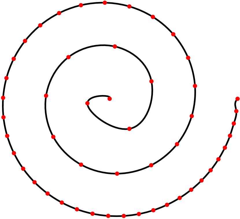
(a) The curve before smoothing

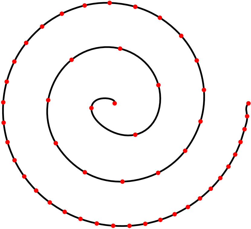
(b) The curve after smoothing

Figure 1: The result of algorithm applied to (4.1). The red dots mark the sample points.

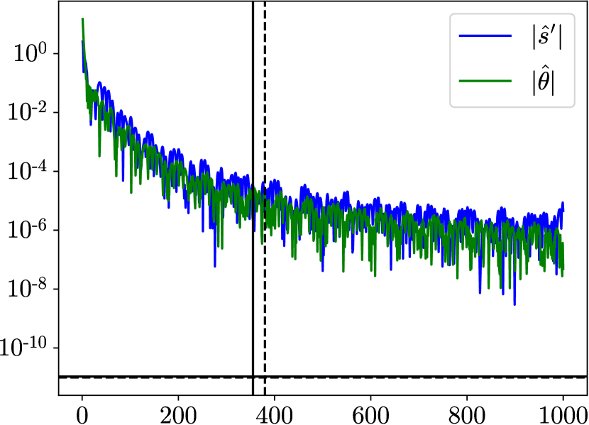
(a) Before filtering

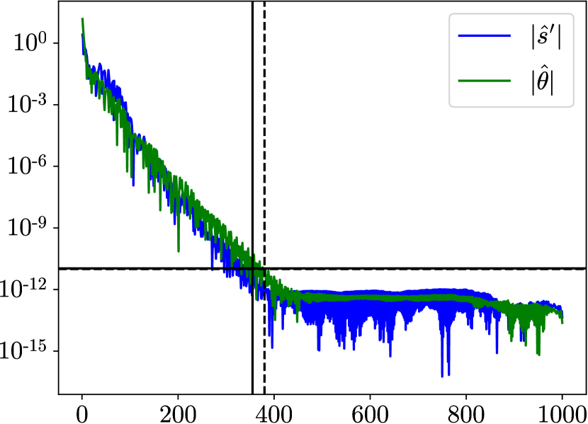
(b) After filtering

Figure 2: Chebyshev coefficients of $s^{\prime}(t)$ and $\theta(t)$ corresponding to Figure 1. The value of $\delta_{s^{\prime}}$ is indicated by a horizontal solid line and the value of $\delta_{\theta}$ is indicated by a horizontal dashed line. The $355$th coefficients of $s^{\prime}(t)$ decays to $\delta_{s^{\prime}}$, indicated by a vertical solid line. The $380$th coefficients of $\theta(t)$ decays to $\delta_{\theta}$, indicated by a vertical dashed line.

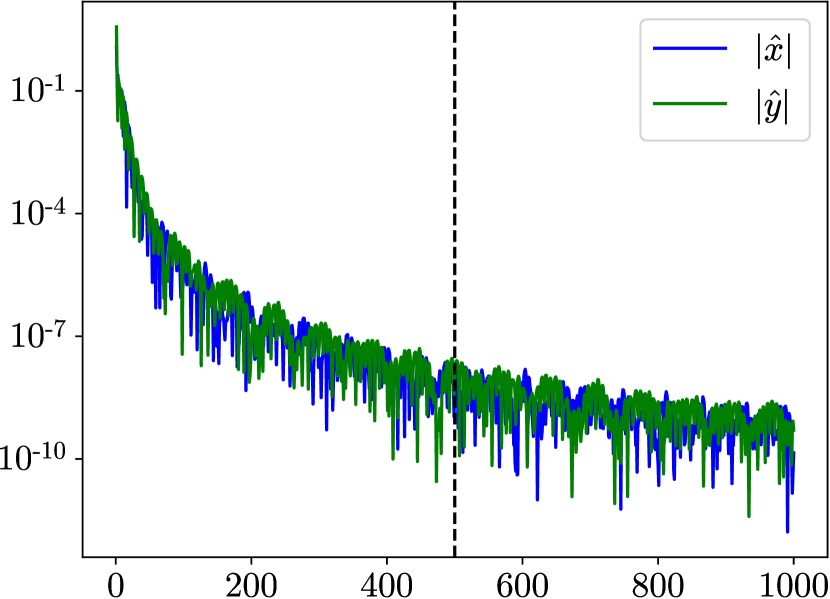
(a) Chebyshev coefficients of the initial curve

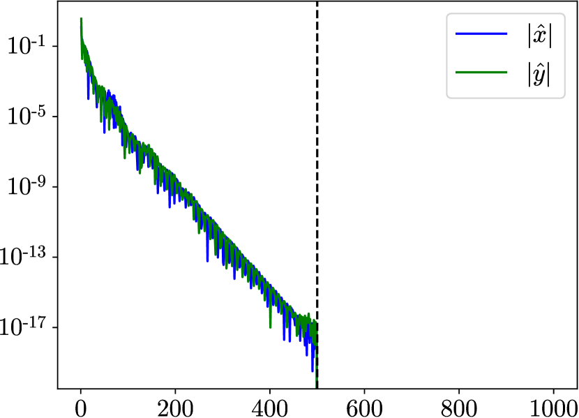
(b) Chebyshev coefficients of the final curve

Figure 3: Chebyshev coefficients of $x(t)$ and $y(t)$ corresponding to Figure 1. The value of $n_{\text{coefs}}$ is indicated by a vertical dashed line.

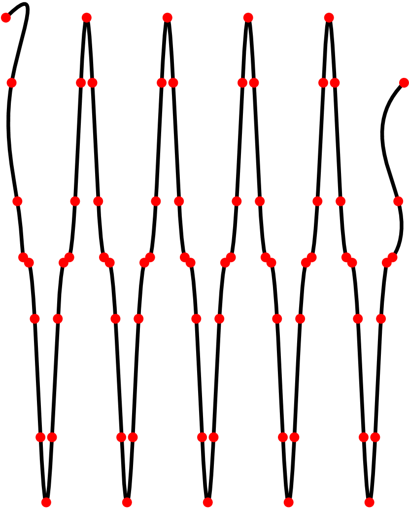
(a) The curve before smoothing

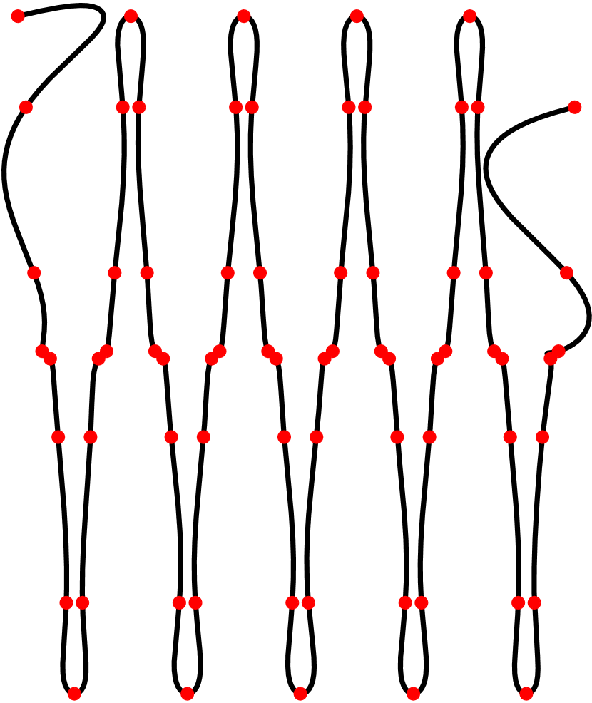
(b) The curve after smoothing

Figure 4: The result of algorithm applied to (92). The red dots mark the sample points.

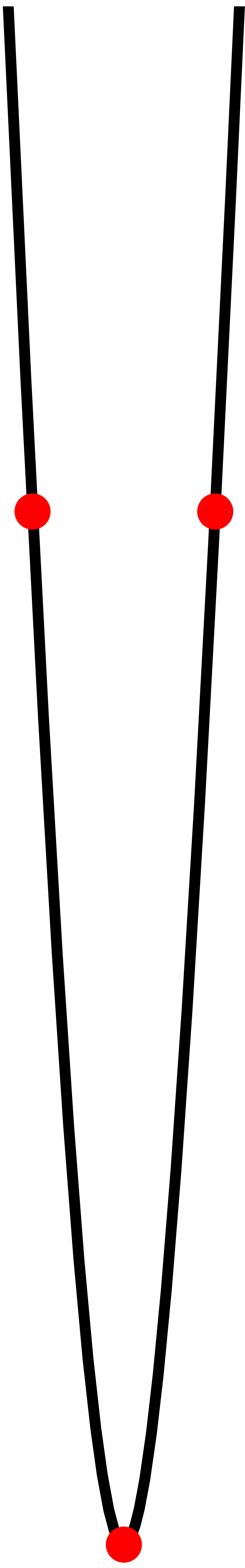
(a) Before smoothing

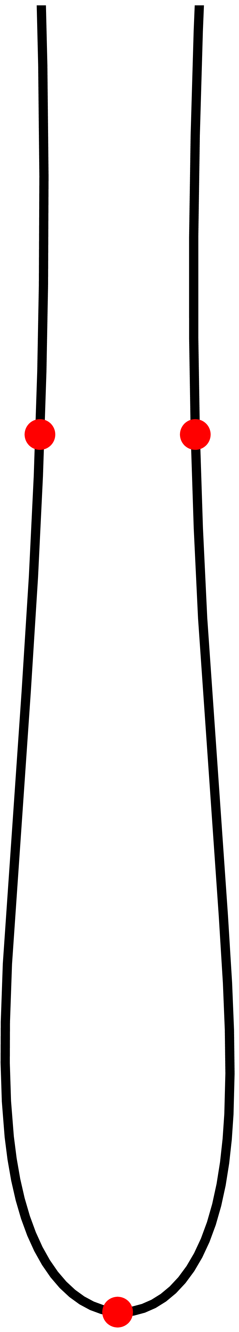
(b) After smoothing

Figure 5: A detail of Figure 4

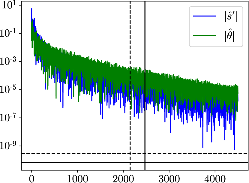
(a) Before filtering

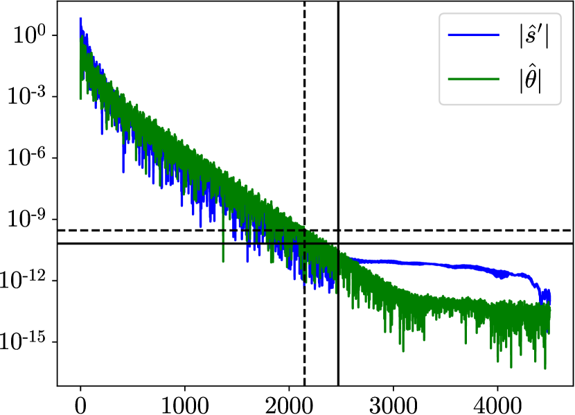
(b) After filtering

Figure 6: Chebyshev coefficients of $s^{\prime}(t)$ and $\theta(t)$ corresponding to Figure 4. The value of $\delta_{s^{\prime}}$ is indicated by a horizontal solid line and the value of $\delta_{\theta}$ is indicated by a horizontal dashed line. The $2472$nd coefficients of $s^{\prime}(t)$ decay to $\delta_{s^{\prime}}$, indicated by a vertical solid line. The $2148$th coefficients of $\theta(t)$ decays to $\delta_{\theta}$, indicated by a vertical dashed line.

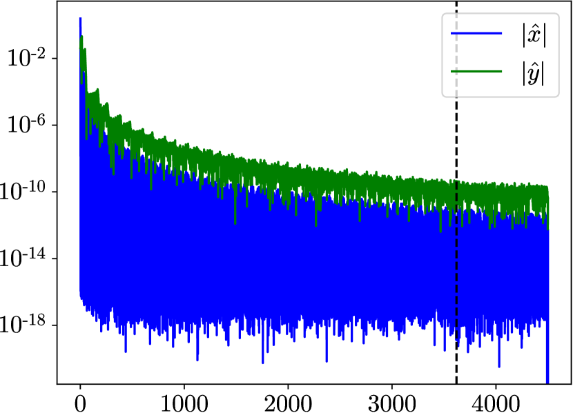
(a) Chebyshev coefficients of the initial curve

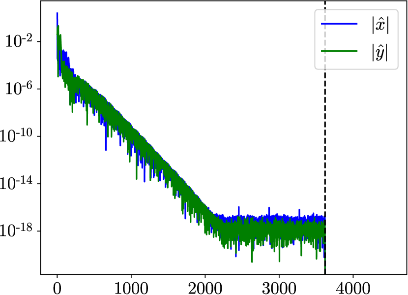
(b) Chebyshev coefficients of the final curve

Figure 7: Chebyshev coefficients of $x(t)$ and $y(t)$ corresponding to Figure 4. The value of $n_{\text{coefs}}$ is indicated by a vertical dashed line.

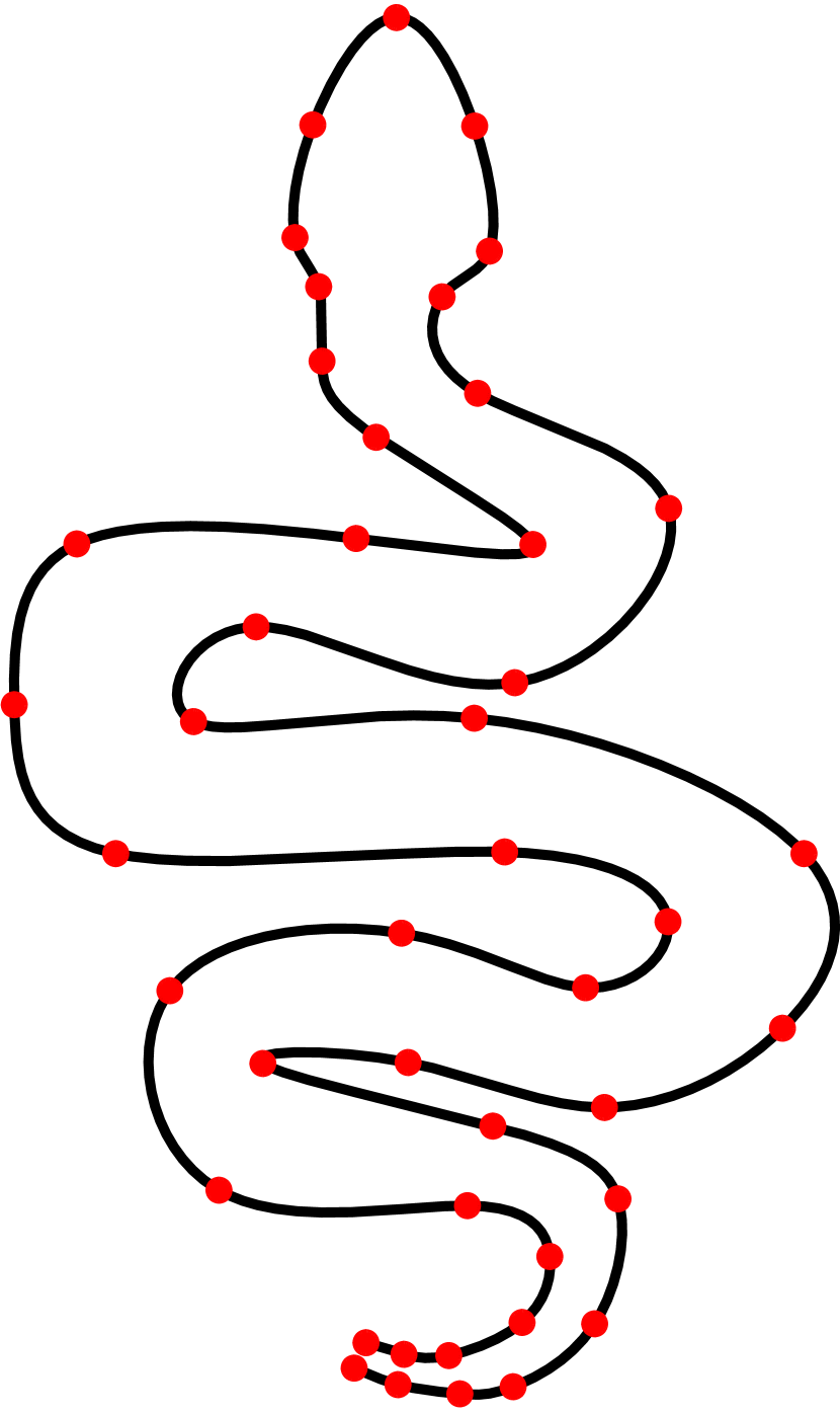
(a) The curve before smoothing

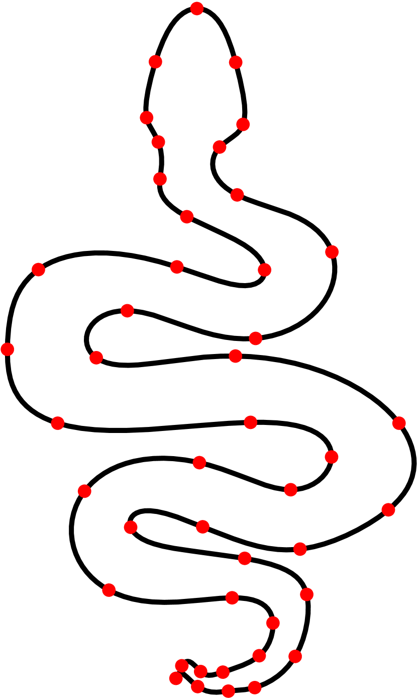
(b) The curve after smoothing

Figure 8: A hand-drawn depiction of a snake shape. The red dots mark the sample points.

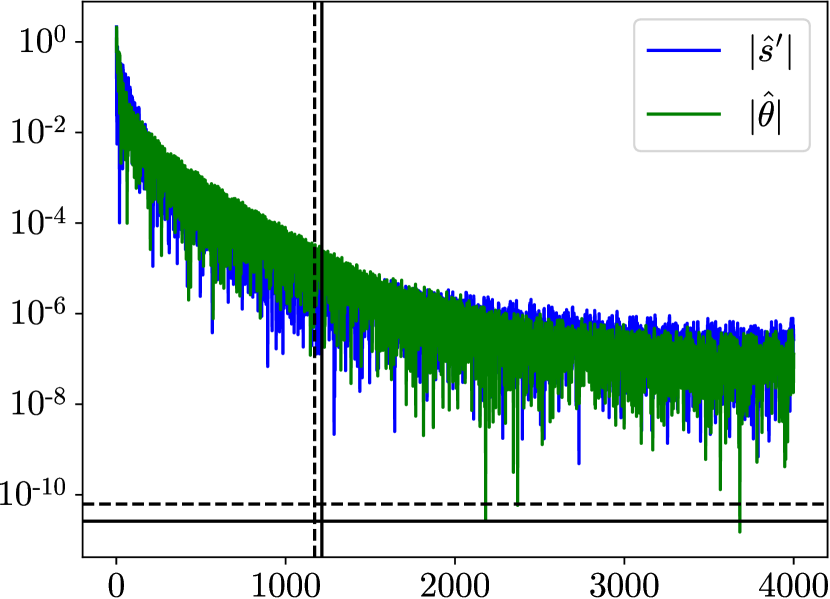
(a) Before filtering

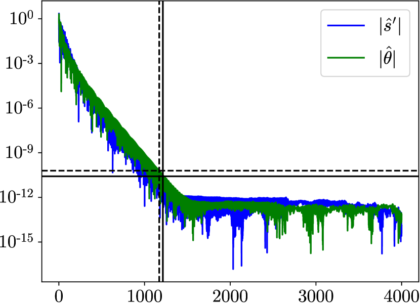
(b) After filtering

Figure 9: Chebyshev coefficients of $s^{\prime}(t)$ and $\theta(t)$ corresponding to Figure 8. The value of $\delta_{s^{\prime}}$ is indicated by a horizontal solid line and the value of $\delta_{\theta}$ is indicated by a horizontal dashed line. The $1214$th coefficients of $s^{\prime}(t)$ decays to $\delta_{s^{\prime}}$, indicated by a vertical solid line. The $1171$st coefficients of $\theta(t)$ decays to $\delta_{\theta}$, indicated by a vertical dashed line.

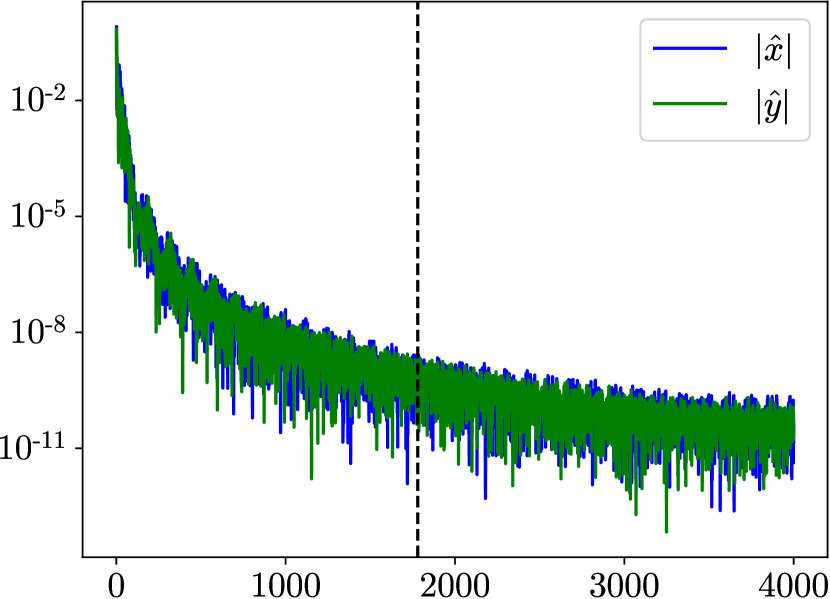
(a) Chebyshev coefficients of the initial curve

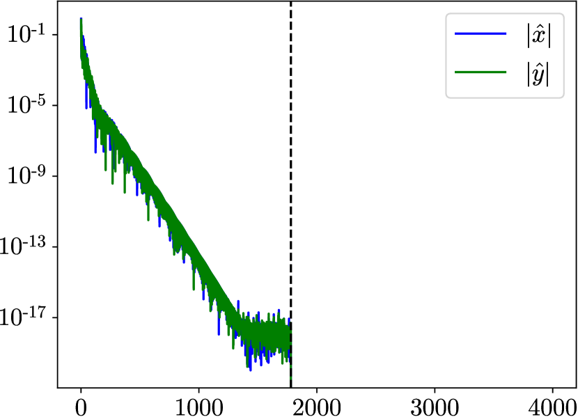
(b) Chebyshev coefficients of the final curve

Figure 10: Chebyshev coefficients of $x(t)$ and $y(t)$ corresponding to Figure 8. The value of $n_{\text{coefs}}$ is indicated by a vertical dashed line.

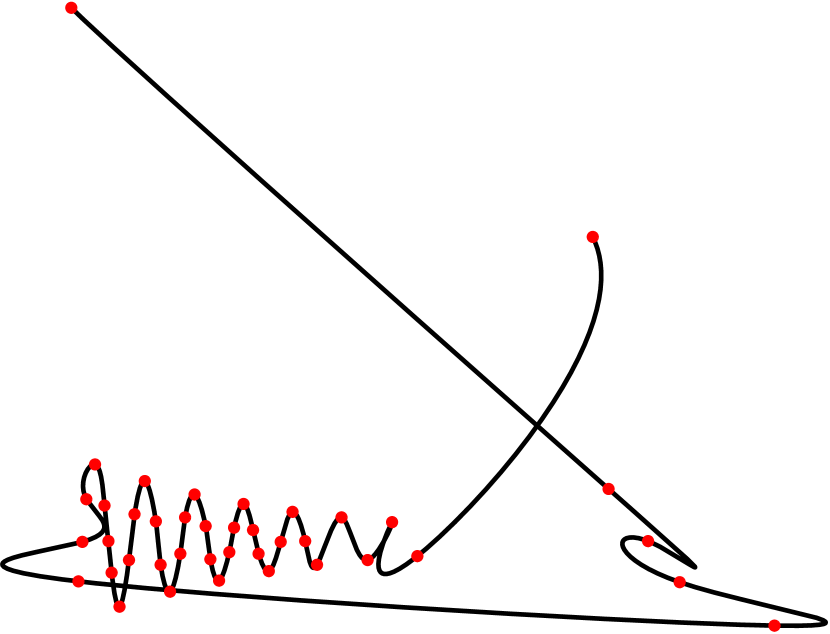
(a) The curve before smoothing

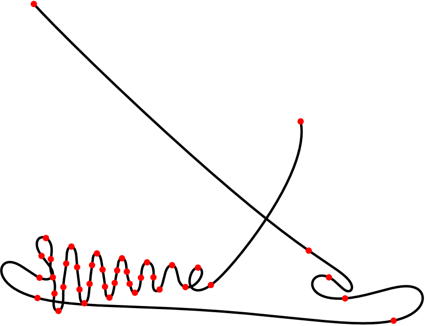
(b) The curve after smoothing

Figure 11: A shape of oscillations that exhibit damping. The red dots mark the sample points.

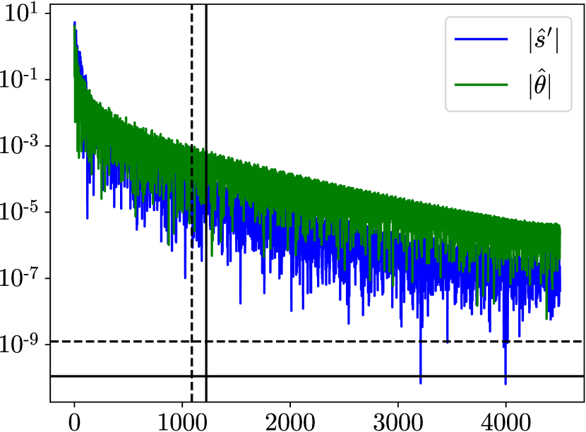
(a) Before filtering

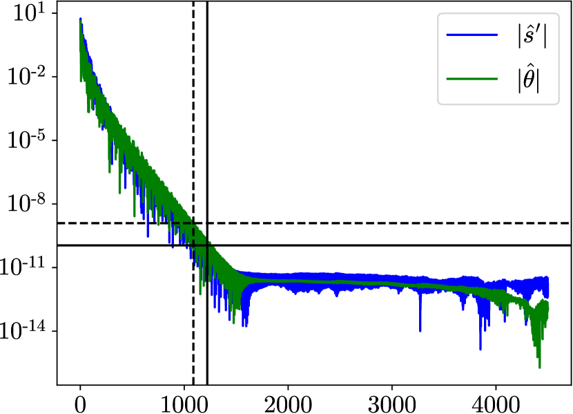
(b) After filtering

Figure 12: Chebyshev coefficients of $s^{\prime}(t)$ and $\theta(t)$ corresponding to Figure 11. The value of $\delta_{s^{\prime}}$ is indicated by a horizontal solid line and the value of $\delta_{\theta}$ is indicated by a horizontal dashed line. The $1222$nd coefficients of $s^{\prime}(t)$ decays to $\delta_{s^{\prime}}$, indicated by a vertical solid line. The $1088$th coefficients of $\theta(t)$ decays to $\delta_{\theta}$, indicated by a vertical dashed line.

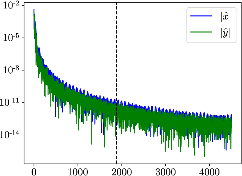
(a) Chebyshev coefficients of the initial curve

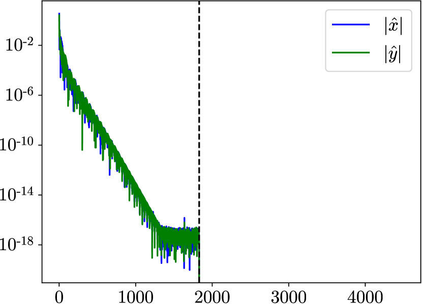
(b) Chebyshev coefficients of the final curve

Figure 13: Chebyshev coefficients of $x(t)$ and $y(t)$ corresponding to Figure 11. The value of $n_{\text{coefs}}$ is indicated by a vertical dashed line.

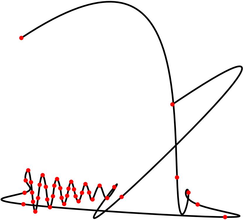
(a) The interpolating curve. The red dots mark the sample points.

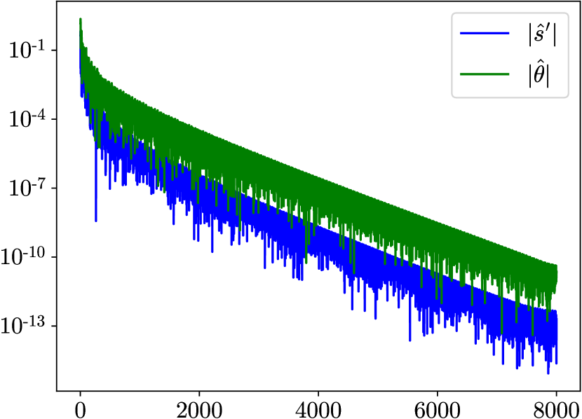
(b) Chebyshev coefficients of $s^{\prime}(t)$ and $\theta(t)$ corresponding to Figure 14(a).

Figure 14: The result of algorithm in [7] applied to the same data points in Figure 11.

Case	$N=1025$	$N=2049$	$N=4097$	$N=8193$
Figure 1	$0.14308\cdot 10^{-02}$	$0.20470\cdot 10^{-02}$	$0.29810\cdot 10^{-02}$	$0.51040\cdot 10^{-02}$

Table 1: Average runtime per iteration, for an open curve, calculated by determining the total runtime for $100$ iterations and dividing by the number of iterations.

4.2 Closed Curve Examples

The first closed curve example is obtained by sampling from the polar representation $(r(t)\cos{\varphi(t)}$, $r(t)\sin{\varphi(t)})$, where

$$\varphi(t) =2\pi t,$$

$$r(t) =(1+\frac{1}{\alpha}\cos{(18\varphi(t))}\sin{(4\varphi(t))},$$ (93)

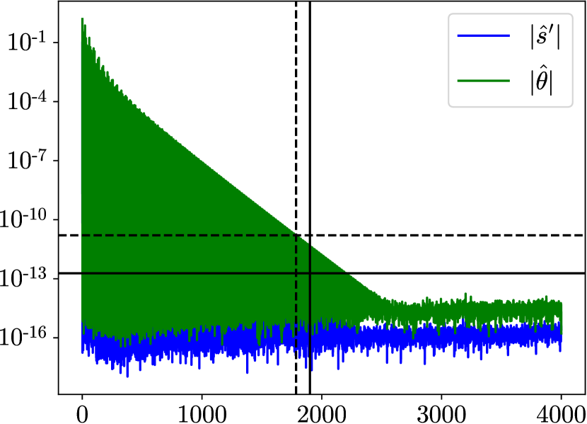
(b) After filtering

Figure 16: Fourier coefficients of $s^{\prime}(t)$ and $\theta(t)$ corresponding to Figure 15. The value of $\delta_{s^{\prime}}$ is indicated by a horizontal solid line and the value of $\delta_{\theta}$ is indicated by a horizontal dashed line. The $1901$st coefficients of $s^{\prime}(t)$ decays to $\delta_{s^{\prime}}$, indicated by a vertical solid line. The $1785$th coefficients of $\theta(t)$ decays to $\delta_{\theta}$, indicated by a vertical dashed line.

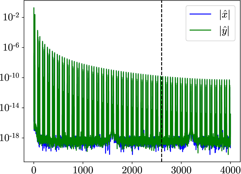
(a) Fourier coefficients of the initial curve

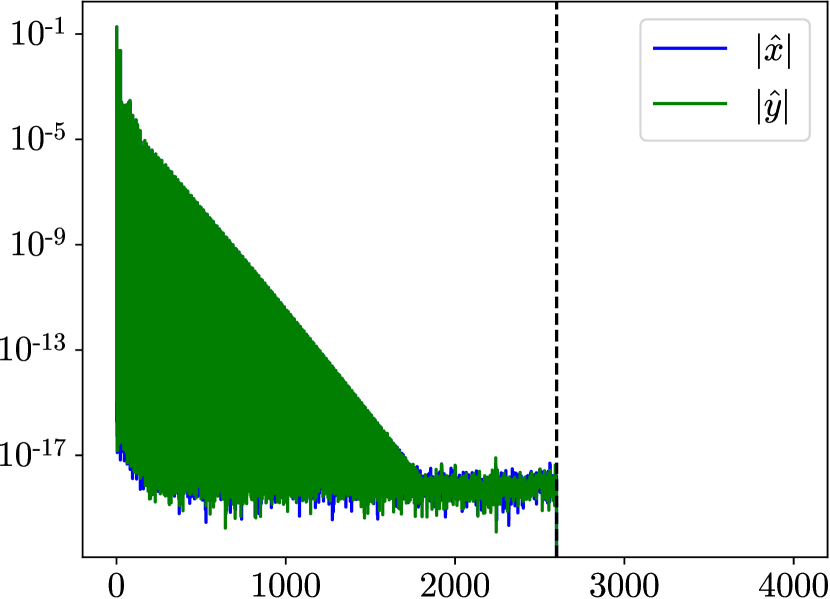
(b) Fourier coefficients of the final curve

Figure 17: Fourier coefficients of $x(t)$ and $y(t)$ corresponding to Figure 15. The value of $n_{\text{coefs}}$ is indicated by a vertical dashed line.

with $t\in[0,1]$, and $\alpha$ is a tuning parameter. The sample data points are scaled so that both their width and height are $1$. We sample the curve (4.2) with $\alpha=2$, $N=8000$ and $n=100$ to obtain the initial curve in Figure 15(a). Applying the algorithm with $n_{\text{iters}}=70$, $h_{\text{filter}}=\frac{1}{35}$, $\epsilon=10^{-16}$, $n_{\text{coefs}}=5200$, $n_{\text{bands}}=12$, we obtained the filtered coefficients of $\theta(t)$ and $s^{\prime}(t)$, as displayed in Figure 16. We find that, after $n_{\text{stop}}=67$ iterations, $5200$ coefficients of $x(t)$ and $y(t)$ are necessary to represent the smooth curve displayed in Figure 15(b), to within an error of $E_{\text{samp}}=0.22453\cdot 10^{-14}$. The magnitudes of the coefficients of both the initial and final curve are displayed in Figure 17.

Remark 4.1.

Note that, since the DFT, $X_{-\frac{N}{2}},\ldots,X_{\frac{N}{2}-1}$, of a real sequence, $x_{0}$, …, $x_{N-1}$, satisfies the relation:

$$X_{k}=\overline{X}_{-k},\qquad k=-\frac{N}{2},\ldots,\frac{N}{2}-1,$$ (94)

we only show the magnitudes of the coefficients, for $k=0$, …, $\frac{N}{2}-1$.

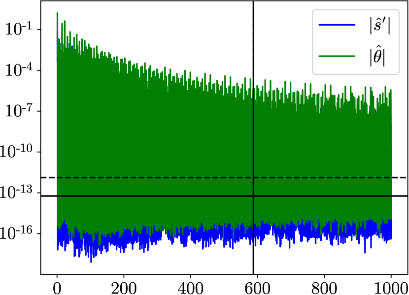
(a) Before filtering

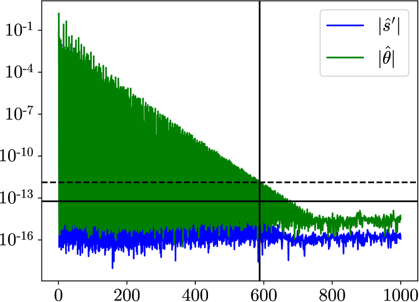
(b) After filtering

Figure 19: Fourier coefficients of $s^{\prime}(t)$ and $\theta(t)$ corresponding to Figure 18. The value of $\delta_{s^{\prime}}$ is indicated by a horizontal solid line and the value of $\delta_{\theta}$ is indicated by a horizontal dashed line. The $588$th coefficients of $s^{\prime}(t)$ decays to $\delta_{s^{\prime}}$, indicated by a vertical solid line. The $588$th coefficients of $\theta(t)$ decays to $\delta_{\theta}$, indicated by a vertical dashed line.

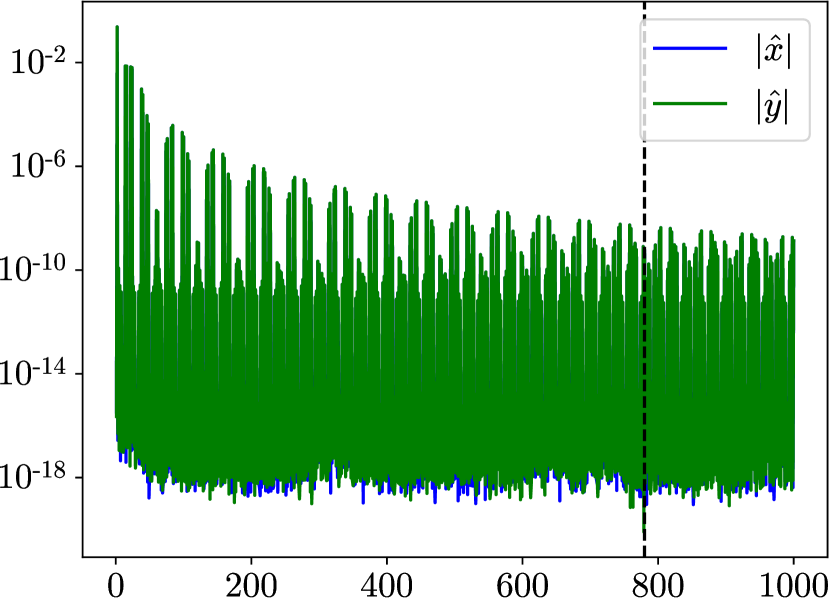
(a) Fourier coefficients of the initial curve

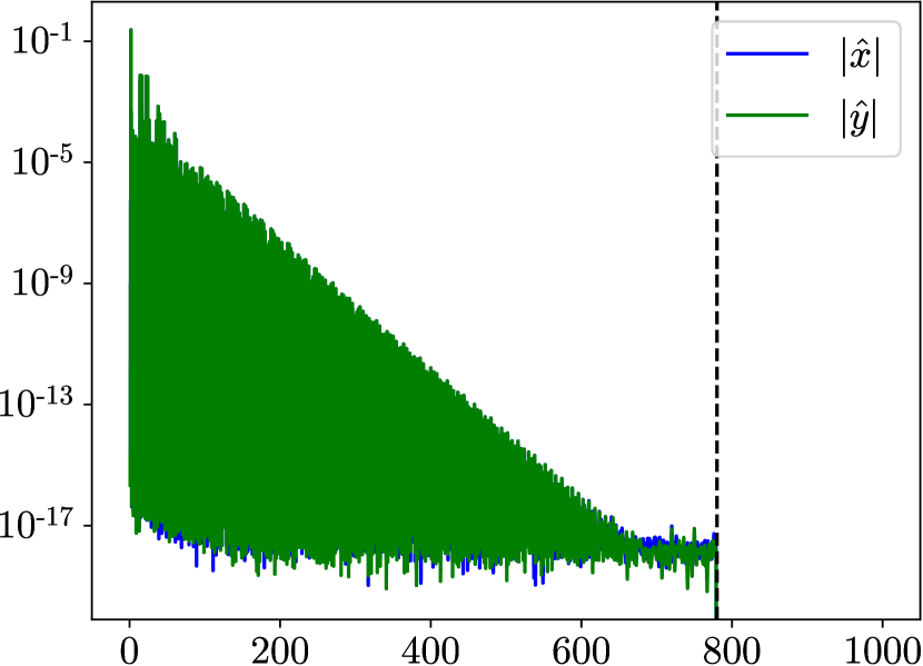
(b) Fourier coefficients of the final curve

Figure 20: Fourier coefficients of $x(t)$ and $y(t)$ corresponding to Figure 18. The value of $n_{\text{coefs}}$ is indicated by a vertical dashed line.

Another example is shown in Figure 18, by sampling the curve (4.2) with $\alpha=8$, $N=2000$ and $n=60$. The sample data points are scaled so that both their width and height are $1$. It is obvious that the curve has fewer wobbles than the previous curve. In this case, we set $n_{\text{iters}}=60$, $h_{\text{filter}}=\frac{1}{35}$, $\epsilon=10^{-16}$, $n_{\text{coefs}}=1560$, $n_{\text{bands}}=8$. The algorithm terminates after $n_{\text{stop}}=34$ iterations, and the error between the final curve and the sample data points is $E_{\text{samp}}=0.11008\cdot 10^{-14}$. The magnitudes of the coefficients of $s^{\prime}(t)$ and $\theta(t)$ before and after filtering are displayed in Figure 19, and the magnitudes of the coefficients of both the initial and final curve are displayed in Figure 20. While the shapes of the curves appear similarly before and after filtering, the coefficients change dramatically.

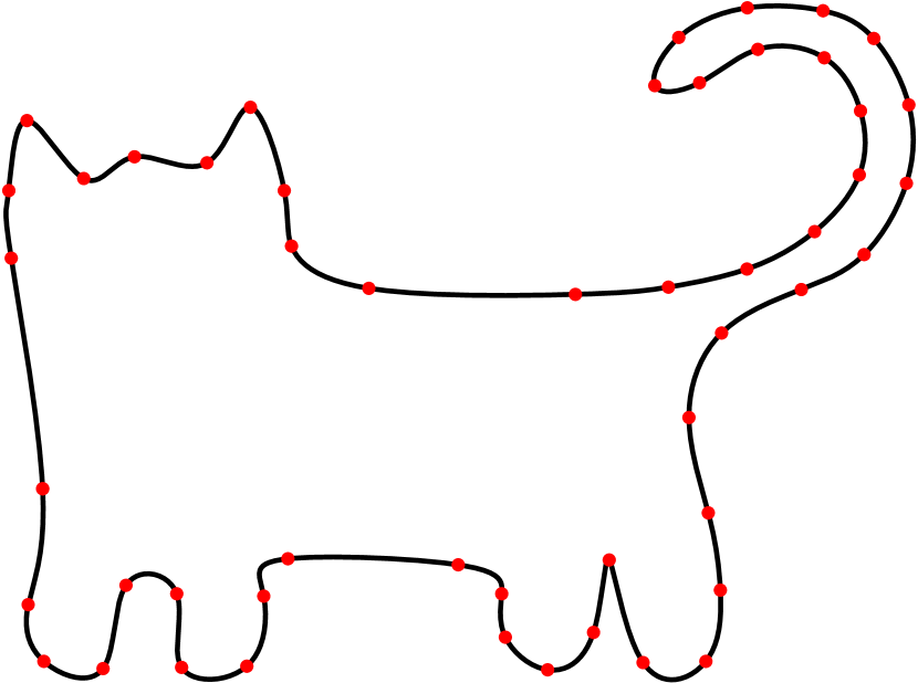
(a) The curve before smoothing

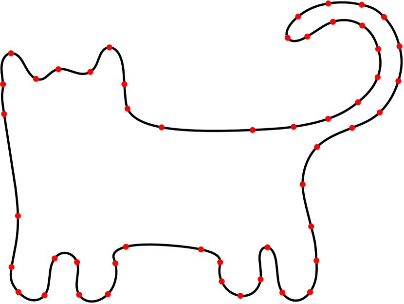
(b) The curve after smoothing

Figure 21: A hand-drawn depiction of a cat shape. The red dots mark the sample points.

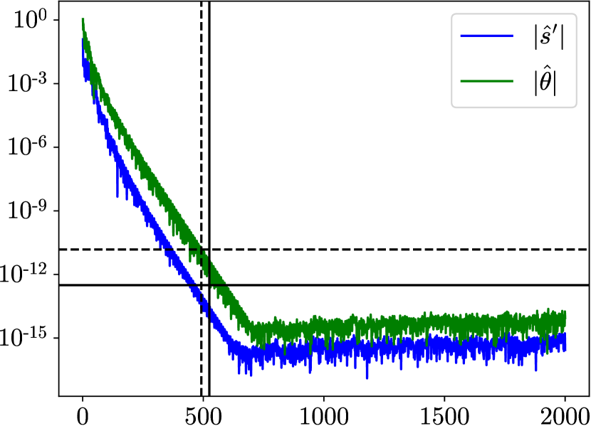
(b) After filtering

Figure 22: Fourier coefficients of $s^{\prime}(t)$ and $\theta(t)$ corresponding to Figure 21. The value of $\delta_{s^{\prime}}$ is indicated by a horizontal solid line and the value of $\delta_{\theta}$ is indicated by a horizontal dashed line. The $525$th coefficients of $s^{\prime}(t)$ decays to $\delta_{s^{\prime}}$, indicated by a vertical solid line. The $492$nd coefficients of $\theta(t)$ decays to $\delta_{\theta}$, indicated by a vertical dashed line.

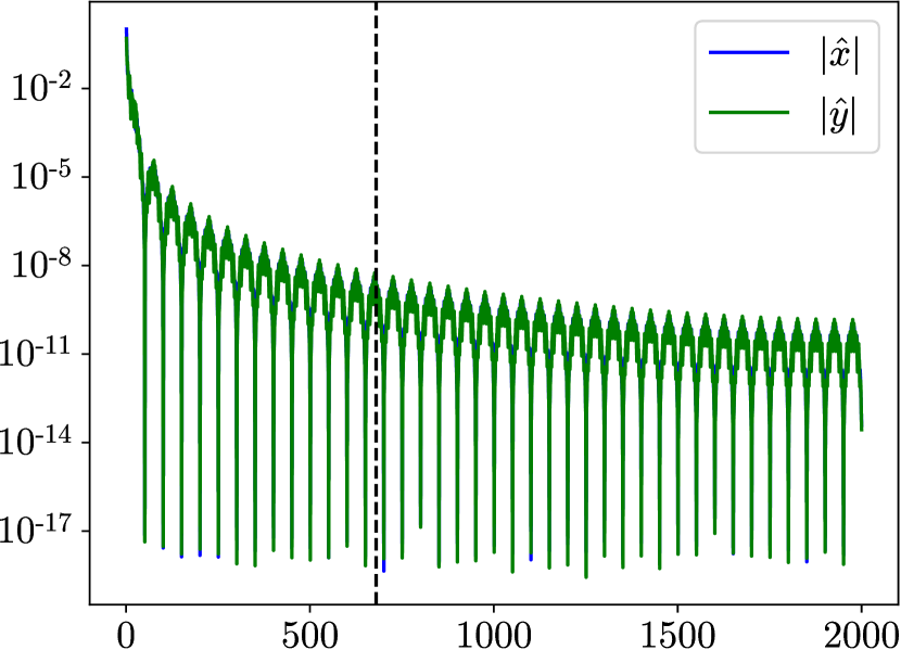
(a) Fourier coefficients of the initial curve

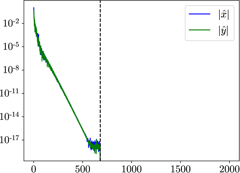
(b) Fourier coefficients of the final curve

Figure 23: Fourier coefficients of $x(t)$ and $y(t)$ corresponding to Figure 21. The value of $n_{\text{coefs}}$ is indicated by a vertical dashed line.

The example shown in Figure 21 has the shape of a cat, corresponding to $n=50$ sample points. We scale the sample data points so that their height is $1$, and discretize the curve with $N=4000$, and set $n_{\text{iters}}=100$, $h_{\text{filter}}=\frac{1}{45}$, $\epsilon=10^{-15}$, $n_{\text{coefs}}=1360$, $n_{\text{bands}}=4$. After $n_{\text{stop}}=98$ iterations, $1360$ coefficients are sufficient to represent the curve, and the error between the final curve and the sample data points is $E_{\text{samp}}=0.64403\cdot 10^{-14}$. The magnitudes of the coefficients of $s^{\prime}(t)$ and $\theta(t)$ before and after filtering are displayed in Figure 22, and the magnitudes of the coefficients of both the initial and final curve are displayed in Figure 23. We observe that the sharp edges on the curve in Figure 21(a) becomes more rounded, and the resulting curve more closely resembles the shape of a cat. Meanwhile, Figure 24(a) is the result of the algorithm in [7] applied to the same data points, with $a=0.4$. The number of coefficients that are necessary to represent $s^{\prime}(t)$ and $\theta(t)$ are displayed in Figure 24(b). As we can observe from Figure 24(a), the curve contains sharp corners, and its visual smoothness is similar to the initial curve displayed in Figure 21(a), prior to applying our algorithm. In contrast, our algorithm eliminates high curvature areas, resulting in a much smoother appearance.

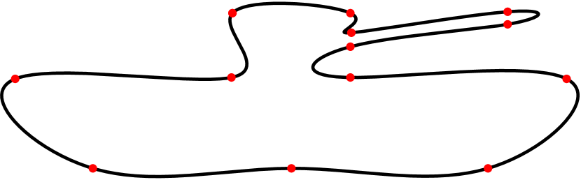
(a) The curve before smoothing

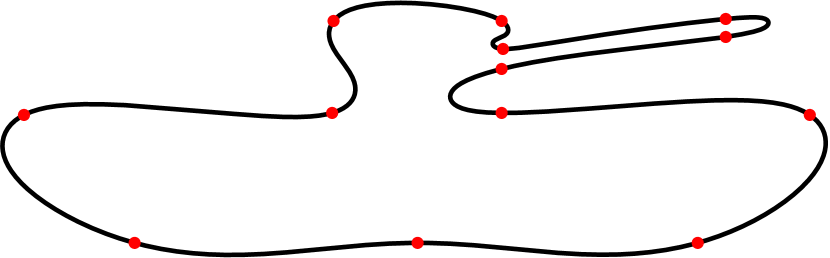
(b) The curve after smoothing

Figure 25: The result of algorithm applied to Figure $4.5$ in [12]. The red dots mark the sample points.

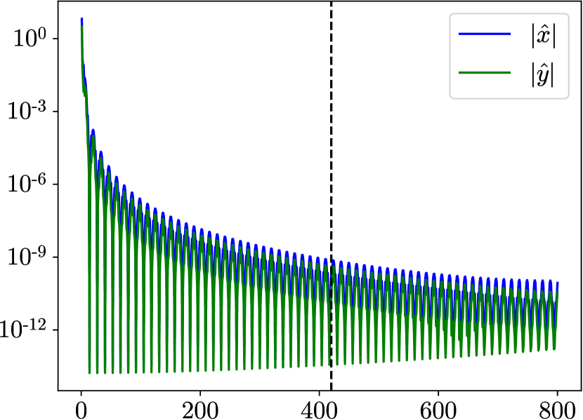
(a) Fourier coefficients of the initial curve

(b) Fourier coefficients of the final curve

Figure 28: Fourier coefficients of $x(t)$ and $y(t)$ corresponding to Figure 25. The value of $n_{\text{coefs}}$ is indicated by a vertical dashed line.

Inspired by Figure 4.5 and Figure 4.3 in [12], we apply our algorithm to the same sample data points to show that our algorithm produces a smoother curve and represents the curve with fewer coefficients. We start with the example in Figure 4.5. The sample data points are scaled so that their width is $1$. With the parameters $N=1600$, $n=13$, $n_{\text{iters}}=80$, $h_{\text{filter}}=\frac{1}{35}$, $\epsilon=10^{-16}$, $n_{\text{coefs}}=840$, and $n_{\text{bands}}=4$, our algorithm produces a curve represented by only $840$ coefficients, while the algorithm of [12] produces a curve represented by $2\cdot 25,000=50,000$ coefficients. The algorithm terminates at the $n_{\text{stop}}=58$th iteration, and the resulting curve passes through the sample data points within an error of $E_{\text{samp}}=0.15713\cdot 10^{-13}$. Notice that the corners in Figure $4.5$ are eliminated and the final curve in Figure 25(b) looks much smoother. We display the magnitudes of the coefficients of $s^{\prime}(t)$ and $\theta(t)$ before and after filtering in Figure 27, and the magnitudes of the coefficients of both the initial and final curve in Figure 28.

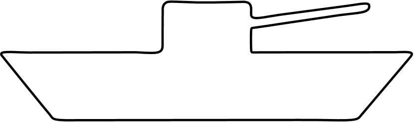
(a) The curve before smoothing

(b) The curve after smoothing

Figure 29: The result of algorithm applied to Figure $4.5$ in [12], with more sample data points. Due to the large quantity and non-uniform distribution of the sample data points, we choose not to display them in the plot.

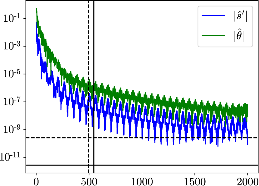
(a) Before filtering

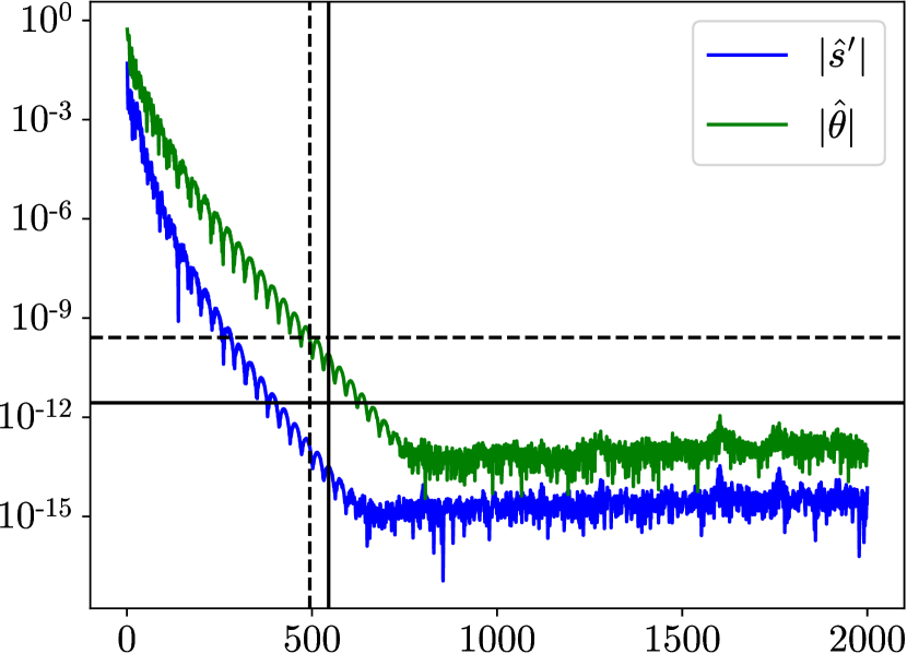
(b) After filtering

Figure 30: Fourier coefficients of $s^{\prime}(t)$ and $\theta(t)$ corresponding to Figure 29. The value of $\delta_{s^{\prime}}$ is indicated by a horizontal solid line and the value of $\delta_{\theta}$ is indicated by a horizontal dashed line. The $545$th coefficients of $s^{\prime}(t)$ decays to the $\delta_{s^{\prime}}$, indicated by a vertical solid line. The $494$th coefficients of $\theta(t)$ decays to the $\delta_{\theta}$, indicated by a vertical dashed line.

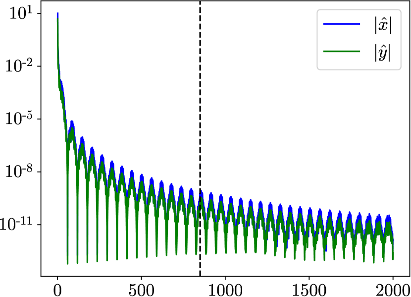
(a) Fourier coefficients of the initial curve

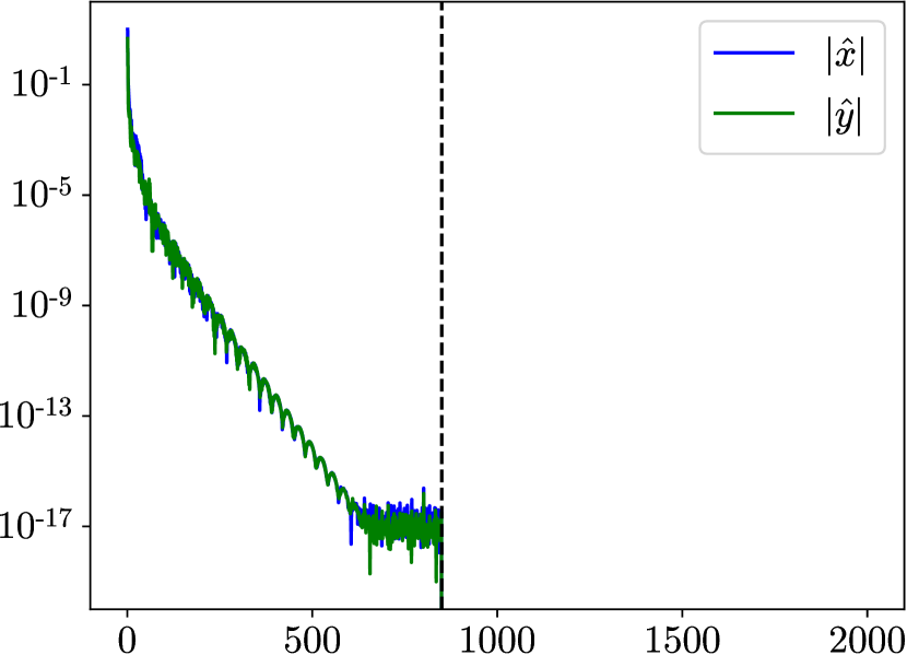
(b) Fourier coefficients of the final curve

Figure 31: Fourier coefficients of $x(t)$ and $y(t)$ corresponding to Figure 29. The value of $n_{\text{coefs}}$ is indicated by a vertical dashed line.

Since the initial curve is constructed by using smooth splines to connect the sample data points, and our algorithm filters the curve further during the filtering process, this causes the shape of the curve to deviate from that of Figure 4.5 in [12]. In order to preserve the shape of the curve in Figure 4.5, we increase the number of sample data points. The sample data points are scaled so that their width is $1$. Applying the algorithm to the curve displayed in Figure 29(a), with $N=4000$, $n=59$, $n_{\text{iters}}=80$, $h_{\text{filter}}=\frac{1}{45}$, $\epsilon=10^{-16}$, $n_{\text{coefs}}=1700$, $n_{\text{bands}}=4$, we obtain $E_{\text{samp}}=0.83564\cdot 10^{-13}$ at the $n_{\text{stop}}=72$nd iteration. The magnitudes of the coefficients of $s^{\prime}(t)$ and $\theta(t)$ before and after filtering are displayed in Figure 30, and the magnitudes of the coefficients of both the initial and final curve are displayed in in Figure 31. It is noteworthy that the shape of the curve has been preserved, while achieving a smoother curve than in [12]. Moreover, the number of coefficients required to represent the curve increases only moderately when compared to those shown in Figure 27.

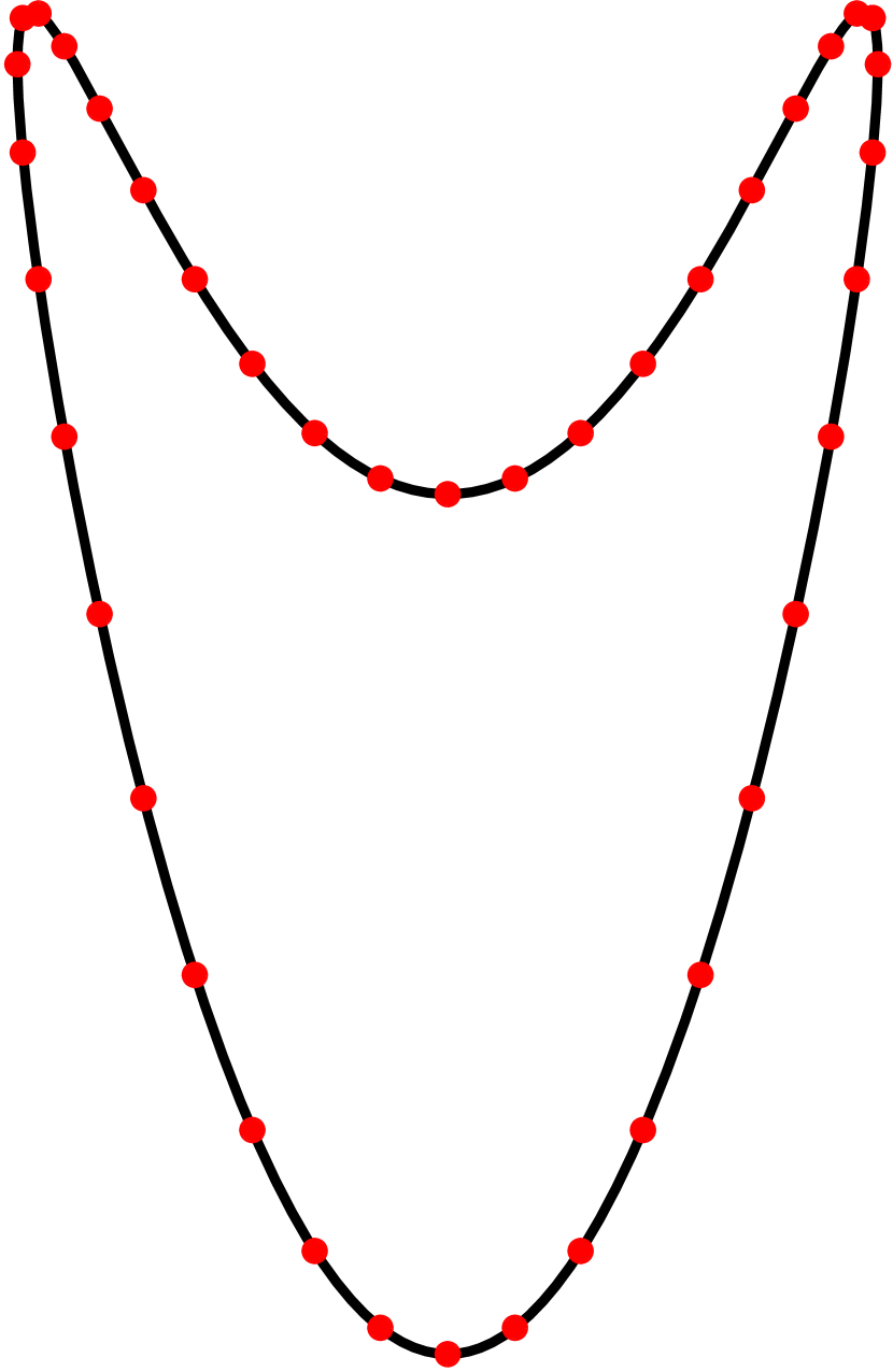
(a) The curve before smoothing

(b) The curve after smoothing

Figure 32: The result of algorithm applied to Figure $4.3$ in [12]. The red dots mark the sample points.

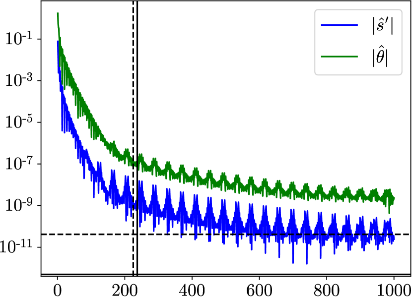
(a) Before filtering

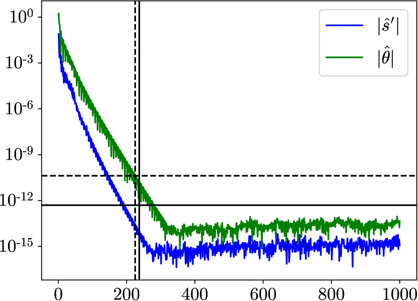
(b) After filtering

Figure 34: Fourier coefficients of $s^{\prime}(t)$ and $\theta(t)$ corresponding to Figure 32. The value of $\delta_{s^{\prime}}$ is indicated by a horizontal solid line and the value of $\delta_{\theta}$ is indicated by a horizontal dashed line. The $237$th coefficients of $s^{\prime}(t)$ decays to $\delta_{s^{\prime}}$, indicated by a vertical solid line. The $225$th coefficients of $\theta(t)$ decays to $\delta_{\theta}$, indicated by a vertical dashed line.

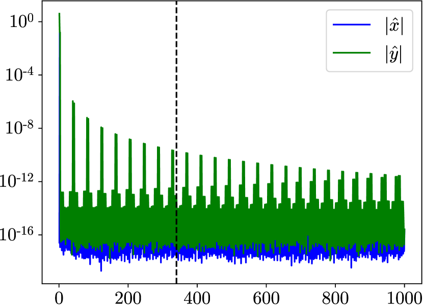
(a) Fourier coefficients of the initial curve

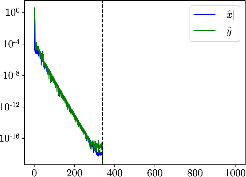
(b) Fourier coefficients of the final curve

Figure 35: Fourier coefficients of $x(t)$ and $y(t)$ corresponding to Figure 32. The value of $n_{\text{coefs}}$ is indicated by a vertical dashed line.

For Figure $4.3$ in [12], we scale the sample data points so that their height is $1$, and apply the algorithm to the reproduced curve in Figure 32(a), with $N=2000$, $n=41$, $n_{\text{iters}}=70$, $h_{\text{filter}}=\frac{1}{40}$, $\epsilon=10^{-16}$, $n_{\text{coefs}}=680$, $n_{\text{bands}}=4$. Although the difference can not be distinguished visually, after $n_{\text{stop}}=55$ iterations, $680$ coefficients are necessary to represent the curve, to within an error of $E_{\text{samp}}=0.15102\cdot 10^{-13}$. The magnitudes of the coefficients of $s^{\prime}(t)$ and $\theta(t)$ are displayed in in Figure 34, and the magnitudes of the coefficients of both the initial and final curve are displayed in in Figure 35. Notice that the algorithm of [12] requires approximately $2\cdot 7000=14,000$ coefficients to fit a curve passing through the same sample data points.

The runtimes per iteration for the first two closed curve cases are displayed in Table  2. We observe that, as in the open curve case, the runtimes are not strictly proportional to $N$.

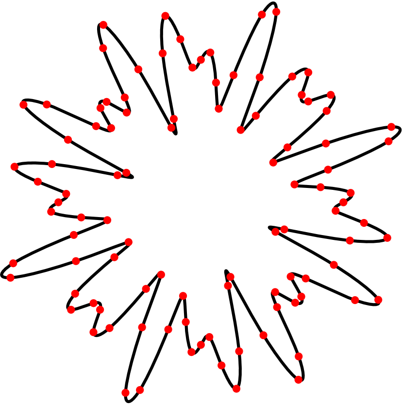
(a) The curve before smoothing

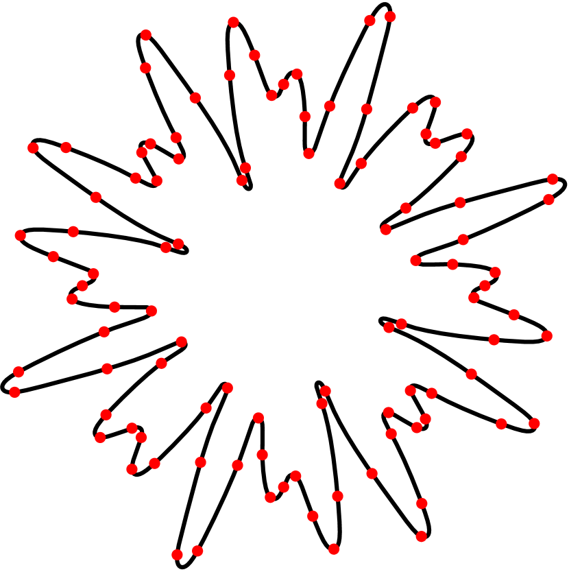
(b) The curve after smoothing

Figure 15: The result of algorithm applied to (4.2) with $\alpha=2$. The red dots mark the sample points.

(a) Before filtering

(a) The curve before smoothing

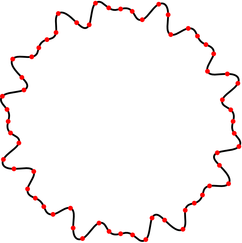
(b) The curve after smoothing

Figure 18: The result of algorithm applied to (4.2) with $\alpha=8$. The red dots mark the sample points.

(a) Before filtering

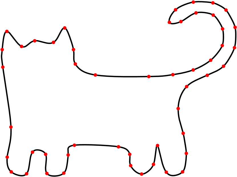
(a) The interpolating curve. The red dots mark the sample points.

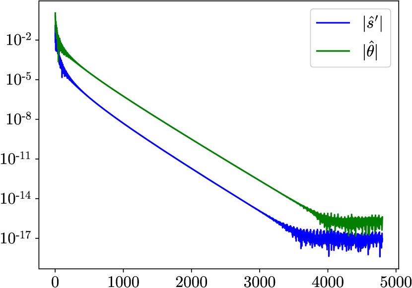
(b) Fourier coefficients of $s^{\prime}(t)$ and $\theta(t)$ corresponding to Figure 24(a).

Figure 24: The result of algorithm in [7] applied to the same data points in Figure 21.

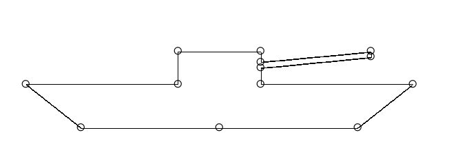
Figure 26: Figure $4.5$ in [12]

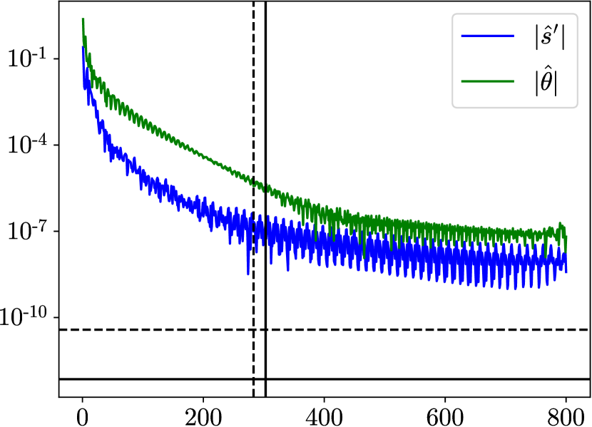
(a) Before filtering

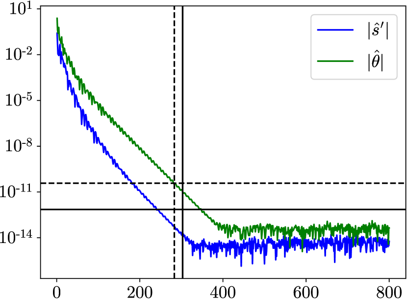
(b) After filtering

Figure 27: Fourier coefficients of $s^{\prime}(t)$ and $\theta(t)$ corresponding to Figure 25. The value of $\delta_{s^{\prime}}$ is indicated by a horizontal solid line and the value of $\delta_{\theta}$ is indicated by a horizontal dashed line. The $303$rd coefficients of $s^{\prime}(t)$ decays to the $\delta_{s^{\prime}}$, indicated by a vertical solid line. The $283$rd coefficients of $\theta(t)$ decays to the $\delta_{\theta}$, indicated by a vertical dashed line.

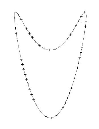
Figure 33: Figure $4.3$ in [12]

Case	$N=1024$	$N=2048$	$N=4096$	$N=8192$
Figure 15	$0.44050\cdot 10^{-03}$	$0.72667\cdot 10^{-03}$	$0.13412\cdot 10^{-02}$	$0.26530\cdot 10^{-02}$
Figure 18	$0.36162\cdot 10^{-03}$	$0.61837\cdot 10^{-03}$	$0.11924\cdot 10^{-02}$	$0.24492\cdot 10^{-02}$

Table 2: Average runtime per iteration, for the first two closed curves, calculated by determining the total runtime for $250$ iterations and dividing by the number of iterations.

5 Conclusion

Our algorithm produces a bandlimited curve passing through a set of points, up to machine precision. It first constructs a $C^{2}$ Bézier spline passing through the points, and then recursively applies a Gaussian filter to both the derivative of the arc length function and the tangential angle of the curve, to control the bandwidth of the coefficients, followed by smooth corrections. The resulting curve can be represented by a small number of coefficients, and resembles a smooth curve drawn naturally by hand, free of ringing artifacts. The algorithm costs O($N\log{N}$) operations at each iteration, and the cost can be further reduced by calling the FFT in the FFTW library [14], in which the speed of the FFT routines is optimized for inputs of certain sizes.

One possible extension of this paper is to design an algorithm for curves and surfaces in $\mathbb{R}^{3}$. The main methodology is still applicable, if we parametrize a curve in $\mathbb{R}^{3}$ by a function $\gamma(t)\colon I\rightarrow\mathbb{R}^{3}$, where $I\subset\mathbb{R}$, in terms of the same parameter $t$ as in this paper, and a surface in $\mathbb{R}^{3}$ by a function $\gamma(s,t)\colon I_{1}\times I_{2}\rightarrow\mathbb{R}$, where $I_{1},I_{2}\subset\mathbb{R}$, in terms of both $s$ and $t$. We can apply the Chebyshev or the Fourier approximation in each parameter, depending on whether the curve or surface is periodic in that parameter, filter the coefficients and add smooth perturbations in a similar way. Another application is to implement the algorithm of this paper as a geometric primitive in CAD/CAM systems. Since primitives are generally defined as level sets of polynomials (see Chapter $2$ of [15]), the techniques in this paper could be used for the constructions of more general $C^{\infty}$ shapes in CAD/CAM systems.

References

- [1] Akima, H. “A new method of interpolation and smooth curve fitting based on local procedures.” J. Assoc. Comput. Mach. 17.4 (1970): 589–602.
- [2] Björkenstam, U., and S. Westberg. “General cubic curve fitting algorithm using stiffness coefficients.” Computer-Aided Design. 19.2 (1987): 58–64.
- [3] Bica, M.A. “Optimizing at the end-points the Akima’s interpolation method of smooth curve fitting.” Computer Aided Geometric Design. 31.5 (2014): 245–257.
- [4] Knott, G.D. Interpolating Cubic Spilnes. Birkhäuser Boston, 2000.
- [5] Runions, A., and F.F. Samavati. “Partition of Unity parametrics: A framework for meta-modeling.” The Visual Comput. 27 (2011): 495–505.
- [6] Piegl, L., and W. Tiller. The NURBS Book. Springer-Berlin, 1995.
- [7] Zhang, R., and W. Ma. “An Efficient Scheme for Curve and Surface Construction based on a Set of Interpolatory Basis Functions.” ACM T. Graphic. 30.2 (2011): 1–11.
- [8] Runions, A., and F.F. Samavati. “CINPACT-splines: A class of Curves with Compact Support.” Curves and Surfaces 2014: Curves and Surfaces. 2015: 384–398.
- [9] Akram, B., U.R. Alim, and F.F. Samavati. “CINAPACT-Splines: A Family of Infinitely Smooth, Accurate and Compactly Supported Splines.” ISVC 2015: Advances in Visual Computing. 2015: 819–829.
- [10] Blu, T., P. Thévenaz, and M. Unser. “MOMS: Maximal-order interpolation of minimal support.” IEEE. T. Image Process. 10.7 (2001): 1069–1080.
- [11] Zhu, Y. “A class of blending functions with smoothness.” Numer. Algorithms 88 (2021): 555–582.
- [12] Beylkin, D., and V. Rokhlin. “Fitting a bandlimited curve to points in a plane.” SIAM J. Sci. Comput. 36.3 (2014): 1048–1070.
- [13] Thompson, M.T. Intuitive Analog Circuit Design. nd ed. Newnes, 2014.
- [14] Frigo, M., and S.G. Johnson. “The Design and Implementation of FFTW3.” Proc. IEEE. 93.2 (2005).
- [15] Hoffmann, C.M. Geometric and Solid Modeling. 2002. See https://www.cs.purdue.edu/homes/cmh/distribution/books/geo.html.
- [16] Joost, M. “Cubic Bézier Splines.” Notes. 2011. See https://www.michael-joost.de/bezierfit.pdf.