Quantitative Verification of Scheduling Heuristics

Abstract

Computer systems use many scheduling heuristics to allocate resources. Understanding their performance properties is hard because it requires a representative workload and extensive code instrumentation. As a result, widely deployed schedulers can make poor decisions leading to unpredictable performance. We propose a methodology to study their specification using automated verification tools to search for performance issues over a large set of workloads, system characteristics and implementation details. Our key insight is that much of the complexity of the system can be overapproximated without oversimplification, allowing system and heuristic developers to quickly and confidently characterize the performance of their designs. We showcase the power of our methodology through four case studies. First, we produce bounds on the performance of two classical algorithms, SRPT scheduling and work stealing, under practical assumptions. Then, we create a model that identifies two bugs in the Linux CFS scheduler. Finally, we verify a recently made observation that TCP unfairness can cause some ML training workloads to spontaneously converge to a state of high network utilization.

1 Introduction

Modern software systems are expected to meet strict operational goals, such as high availability and good performance. However, when subject to unforeseen workloads or operating environments, these systems can be left exposed to corner cases where they fall well short of their goals. The overall performance of the system is critically impacted by scheduling algorithms since they decide how system resources are allocated. As a result, these algorithms have received significant attention from academia and industry.

This paper argues that although scheduling algorithms control complex systems and exhibit complex behaviors, they often have a simple mathematical description. This opens the possibility of using formal verification techniques to guarantee their robustness under arbitrary, pathological, scenarios. Conventional approaches to ensuring robustness, such as testing and fuzzing, require workloads that can trigger all potential problems. These can be difficult or even impossible to build (see §2.1). On the other hand, theoretical tools (e.g., queueing theory and control theory) offer the ability of deriving bounds on the performance of such algorithms. However, they require making lots of oversimplifying assumptions, leading to results that don’t necessarily reflect the algorithm’s performance in practice. In contrast, verification can guarantee performance for all workloads with a simple but accurate description of the algorithm under study.

Formal verification has grown in popularity in recent years, with frameworks for verifying key-value stores [7, 22, 9], network configurations [12, 5, 11, 27], compilers [26, 30, 24, 29], and more. However, most efforts focus on verifying qualitative properties related to correctness, such as safety and liveness. In contrast, proving quantitative properties that provide guarantees on performance has received less attention.

To that end, this paper presents a method for encoding scheduling heuristics, the systems in which they operate, and the performance property to be tested (e.g. work conservation or near-optimality) in an SMT solver. The solver can then either prove that a property always holds or provide a concrete workload where it is violated. Since solvers can quickly and efficiently explore a large number of workloads and system behaviors, they can help us understand complex behaviors that would be difficult or tedious for humans to analyze.

To limit complexity of the analysis while still maintaining accuracy, we model only the parts of the surrounding system that directly interact with the heuristic. Our models overapproximate the system by capturing a superset of system behaviors. Thus, if the model does not contain any behaviors that cause the algorithm to violate the desired property, we can be sure that the real system will not exhibit such behavior either. The principles we adopt (see §3) allow us to reason about complex systems in a clear and concise way.

To illustrate these principles concretely and demonstrate generality, we include four case-studies. The first two prove bounds on the optimality of shortest remaining processing time (SRPT) schedulers and work stealing, demonstrating that our tool can provide insights for well-studied algorithms by relaxing assumptions made in theoretical models. To go beyond the classical theoretical results, we study the performance of SRPT when preemption is not allowed and tasks can block. Further, we study the performance of work stealing algorithms while accounting for context switching costs.

Our third case study is concerned with the performance of the Linux CFS load balancer. In particular, we check if the algorithm is work conserving, reproducing a bug that was recently identified by the community. Further, we identify a new bug that can lead to the violation of the work conservation property. Finally, we show that our approach may not be limited to CPU schedulers by verifying a recent observation [37] that TCP unfairness can cause flows to synchronize to a schedule where they efficiently occupy a shared link.

This paper’s central thesis is that, using our modeling approach, it is possible to quickly and easily analyze scheduling algorithms and draw useful conclusions about their behavior in the real world. The most challenging aspect of scheduler analysis is still asking the right questions and interpreting the answers. However, automation can make this process easier and more reliable. We invite the community to incorporate performance verification as part of their workflow when designing scheduling algorithms.

2 Motivation

2.1 The Problem of Analyzing Heuristics

Heuristics, by definition, are imperfect. However, experts design them to produce results with reasonable performance. The typical way to evaluate the performance of a heuristic is through thorough benchmarks and fuzzing, which show that the heuristic performs well in a wide range of scenarios. These benchmarks can give confidence in the heuristic, but they do not provide guarantees on its worst-case performance. Without guarantees, heuristics can have corner cases that can lead to poor performance, wasted debugging efforts to identify the heuristic as the cause of the problem, and decreased overall reliability of the system.

As an example, we will use the load balancer in the Linux CFS scheduler to illustrate our argument. The Linux load balancer implements complex heuristics to decide which tasks should be moved to which CPU in order to balance the load between CPUs, distribute idle CPU cycles, give each task a fair share of CPU time, avoid moving tasks too much, and respect cache and NUMA placement when moving tasks. Due to its complexity, it is reasonable to question whether the load balancer is work-conserving and fair.

It has been demonstrated repeatedly that the answer is “no”. Many of the identified issues were caused by the algorithm itself, not just the implementation. For example, prior work found that CPUs may remain idle for a long time, even when other cores are overloaded with a large number of active tasks, due to an inadequate method for quantifying the load of a group of CPUs [31]. While these were later fixed, other performance bugs remain. For instance, we discovered a new bug where CPUs can remain idle even with a large number of runnable tasks, because of a spurious check that forces the balancer to return early (see §6.2.2). This occurs despite mechanisms designed apparently to prevent this scenario.

Identifying such performance bugs using conventional methods is a major undertaking. Typically, experienced users or developers observe anomalous behavior when using the heuristic over an extended period of time. Such observations prompt a more methodical effort by the community to reproduce the bug, leading to efforts that can require hours or even days of experimentation. For example, the complete rewrite of the Linux load balancer in v5.5 took several months of careful manual scrutiny by the community to prevent bugs [15].

Not all heuristics are based solely on the designers’ intuition. Many are supported by solid theoretical results that prove the optimality of the heuristic or a version of it under simplifying assumptions. For example, there are strong theoretical bounds on the performance of work stealing algorithms. The models used to prove these bounds ignore practical considerations like the context switching costs [6]. Translating these algorithms to real-world systems results in much more variable performance than is guaranteed by theory, and this has become a active area of research [34, 18, 32]. Designers need systematic guidance to decide whether work stealing is right for them.

There is a tension between two objectives when evaluating heuristics: 1) fidelity of the evaluated heuristics and workloads with respect to the real system, and 2) confidence provided by the evaluation methodology. Theoretical approaches have low fidelity because they rely on simplifications that make the problem tractable for human reasoning. Benchmarks and fuzzers provide higher fidelity by evaluating the actual implementation of the heuristic, but they compromise on confidence by not providing formal guarantees. In this work, we aim to provide a practical tool that offers high confidence in the performance of heuristics without sacrificing fidelity.

2.2 Quantitative Verification

In deploying a scheduler in real-world settings, a system designer or operator may be interested in several questions pertaining to the performance of the scheduling heuristics. We identify three broad classes of such questions:

Q1: Boolean questions about performance. Examples include whether a scheduler is work-conserving, or fair. Answers to these questions could either be that the scheduler satisfies the property in question, or a counterexample showing a valid schedule that breaks the property. These types of questions help the designer ensure the correctness of their design, and identify corner cases missed by the heuristic.

Q2: Comparison with an Oracular Scheduler. When designing a heuristic, it’s typically helpful to know how the heuristic compares to an optimal, oracular scheduler with complete offline knowledge of inputs that can even solve NP-complete problems. Although such an oracular scheduler is impractical, comparing to it helps identify room for improvement and define bounds on the performance of the heuristic. For example, we may desire to define a bound on the performance of the studied heuristic (e.g., it takes at most twice as long as optimal to finish all tasks).

Q3: Precise workload characterization. Heuristics based on theoretical results will perform optimally when operating in settings or on workloads that match the assumptions made in the theoretical model. The same performance might hold for a broader class of workloads, but might also break for other classes of workloads. Similarly, benchmarking and fuzzing can only evaluate a heuristic for specific and finite number of workloads. A heuristic designer will typically be interested in systematically characterizing workloads (as opposed to experimenting with different canonical workloads on a trial-and-error basis) for which the heuristic performs poorly.

Recent advances in verification tools provide an avenue for efficient verification of a wide range of properties. In our context, given a model of the heuristic in question, we interpret “correctness” to mean achieving a quantitative performance criterion, thereby helping answer questions of type Q1. Further, existing verification tools can find assignments that optimize a quantitative measure, allowing us to compare the performance of an encoded heuristic to that of an oracular scheduler. Finally, given a performance metric, we can answer questions of type Q3 by using verification tools to find workloads which perform poorly according to the metric in each of several different specified workload classes.

Heuristic	Queries	Events	Overapproximation
Single-core SRPT Scheduling (§4)	Comparison to an oracle scheduler for various objectives	Tasks changing their states from ready to running to blocking	Causes of blocking and task profiles
Work Stealing (§5)	Characterizing the impact of context switching cost on performance	Start and end of individual tasks in a DAG	Context switching cost
Linux CFS Load Balancer (§6)	Work conservation	Periodic load balancing ticks	Changes in the states of tasks between ticks
Ring Reduce Scheduling (§7)	Achieving high network utilization	Start and end of flows	Behavior of congestion control algorithms

Table 1: A summary of the application of the modeling methodology to four scheduling heurisitics.

3 Methodology

Our main contribution is defining a clear methodology for scheduling heuristic designers to use formal verification tools to debug and better understand the performance of their designs. A designer expresses environment constraints (i.e., CPUs and a task model), a scheduling algorithm (or heuristic), and a performance query. Queries ask whether some performance property is always true for the given scheduling algorithm. If a counterexample exists, it helps the user identify corner cases that can break the studied algorithm. If there is no counterexample, then we have successfully verified the behavior encoded by the query. To answer queries we use Z3, a Satisfiability Modulo Theories (SMT) solver [10]. To keep our models tractable, we only use the theory of linear real arithmetic. Table 1 provides a summary of how our methodology is applied to four different scheduling algorithms. We adopt three design tenets for our models.

Overapproximation not oversimplification. Reasoning about the complexity of a full system is intractable, whether using automated tools or conventional analytical tools. Thus, abstraction is a necessary step. Conventional analytical tools tackle that abstraction with simplifying assumptions, favoring human tractability over soundness. Formal verification, by contrast, favors soundness. Formal verification models tend to overapproximate systems; i.e., the set of possible model behaviors is a superset of the possible behaviors of the modeled system. Hence, any theorems proved in the overapproximated model are also true for the real system. However, counterexamples produced by the model require human inspection to ensure that they are also possible in the underlying system. In our experience, all counterexamples we encountered have a real-world counterpart.

Our methodology is to overapproximate all behavior external to the scheduling algorithm. For example, all blocking calls (e.g., networking, storage, or synchronization) that force a thread to yield a CPU core can be treated collectively as one, allowing a task’s blocking time to have a wide range of values. The solver can then choose any value for the blocking time a thread faces. Despite networking and storage calls typically having bounded latencies, overapproximation helps us avoid making any assumptions about their behavior, allowing us to make general conclusions about the scheduling algorithm.

Overapproximating external behavior makes the system easier to model for the user. In particular, it allows users to focus on modeling the details of their algorithm while the solver picks the behavior of components external to the modeled system. Further, reducing the volume of details makes user–created models more concise. In all of the case studies presented here, for example, the SMT constraints are generated by less than 1,000 lines of Python.

Event-based modeling. Schedulers determine the ordering and time of execution of tasks. There are multiple ways to encode their behavior. As discussed above, we overapproximate all behavior not integral to the heurstic. However, this leaves an important question: how should we model the details of complicated heuristics with many steps and states? Capturing every step and state in a heuristic creates intractable models. A more tractable approach is to discretize time, allowing the automatic solver to capture all possible state transitions that can happen between two timesteps. This approach is intuitive and has been used before to model, for example, the performance of congestion control algorithms [2]. However, this modeling approach suffers from several downsides. First, it limits the time span captured by the model, reducing the scalability of the model. Second, it requires introducing complex constraints to ensure that only valid state transitions, including scheduling decisions, are made between two time steps.

By contrast, our approach relies on identifying key events in schedules produced by a heuristic (e.g., the point in time when a thread blocks). Where necessary, we represent a state with two events: its starting and finishing times. The automated solver can assign arbitrary time values to events, enabling it to capture arbitrarily large time spans. In addition, an algorithm makes scheduling decisions at a particular event, meaning that scheduling behaviors need only be encoded relative to events, potentially simplifying the model.

Unconstrained initial conditions. Event-based modeling limits the number of tasks and events that a model captures, leaving a critical question open: How can a small number of events provide useful insights about complicated heuristics? Testing a scheduling heuristic for violations of a given performance property using benchmarks or fuzzing requires the identification of a concrete task workload under which the heuristic fails. Such a workload is likely to be complex and difficult to analyze, even if only a few of its events cause the property violation. Our approach solves this problem by letting the solver pick arbitrary initial conditions for the system. Compared to a concrete workload under the testing approach, the solver may choose initial conditions corresponding the state of the system just before the events which caused the property violation. In this sense, unconstraining initial conditions allows us to jump past irrelevant events which a benchmarking or fuzzing approach would have to exhaustively consider.

4 Case study: Single Core SRPT Scheduling

We begin with the simplest case study: shortest remaining processing time first (SRPT) on a single processor. It is well known that SRPT is optimal with respect to average time to completion [40]. However, proofs of optimality assume both preemption and no task blocking, for example, to perform IO operations. Later work on queueing theory has provided bounds on the average running time of tasks in a system with general load [3], and investigated the fairness implications of SRPT [4]. The performance of non-preemptive schedulers has also been investigated [1], but not with blocking.

We fill this gap for a simple non-preemptive SRPT scheduler by providing a model which can be used to verify performance properties without prior expertise. For a simple system with a single core and plain SRPT scheduling, we try to understand SRPT’s performance when tasks can block.

4.1 Model

(a) Modeled state machine of a task

(b) Mapping the state machine to an event-based model in time

Figure 1: Task model, showing the model of a single task

We focus on the context of a single core where tasks can alternate between the states of running and blocking and no preemption is allowed. This context is reflective of many RPC execution settings where threads run to completion and only yield when they make blocking calls [34, 18, 44]. Within this context, a task can be in one of three states: ready, running, or blocking, as shown in Figure 1(a). Instead of modeling states explicitly, we identify two events corresponding to the passage of a task through each state: the time when it enters the state and the time it leaves. We call one passage through the state cycle a step; a step has 6 events, two each for ready, running, and blocking as shown in Figure 1(b). We overapproximate real systems by allowing events to happen at arbitrary points in time subject only to constraints enforced by our context (i.e., having a single core). We constrain the system such that only one task can be running at any point in time. Under this model, a schedule is simply an ordering on the time each task enters each state.

Tasks. We consider a model with $n$ tasks $T_{1},\dots,T_{n}$. We limit the number of events in the model by fixing the number of steps $s$ per task. A step is one ready–running–blocking cycle in Figure 1; each task has six events per step. We define a task $T_{i}$ as a tuple of $(L_{i},D_{i},R_{i},B_{i})$, where $L_{i}>0$ is the total length of the task (i.e., the sum of all the time it spends running). $D,R,B\in(\mathbb{R}\times\mathbb{R})^{s}$ are sets of pairs that define the start and end of ready, running, and blocking periods, respectively. We denote these with $D=\left\{\left(Ds_{i}^{j},Df_{i}^{j}\right)~{}\mid~{}1\leq j\leq s\right\}$, where $Ds_{i}^{j}$ is the start of the ready event of task $i$ in step $j$ and $Df_{i}^{j}$ is the end of the same ready event. We define $R$ and $B$ similarly.

The model includes constraints that ensure the proper timing of all events. At the task level, we ensure that the sum of the running times per task is equal to its length. Further, tasks must always be in one of the three states, and must proceed from waiting to running to blocking in that order. Formally:

$$\forall i\quad(Df_{i}^{j}=Rs_{i}^{j}<Rf_{i}^{j}=Bs_{i}^{j}\leq Bf_{i}^{j}), 1\leq j\leq s$$

$$\forall i\quad(Bf_{i}^{j}=Ds_{i}^{j+1}), 1\leq j<s$$

Scheduler. Since a schedule is simply a valid ordering on events, we can represent a scheduling algorithm as a constraint on task variables. SRPT allows a task to run iff that task has the least remaining processing time or all tasks with less remaining time are blocking. Formally, let the remaining processing time of task $i$’s step $j$ be $e_{i}^{j}=L_{i}-\sum_{k=0}^{j}(Rf_{i}^{k}-Rs_{i}^{k})$. SRPT can be defined as on ordering on running times, subject to the remaining time of each task

$$\forall i,l\leq n\hskip 7.22743pt\forall j,k\leq s\qquad(Rs_{i}^{j}<Rs_{l}^{k})\iff$$

$$\quad\big{(}e_{i}^{j-1}\leq e_{l}^{k-1}\wedge Rf_{l}^{k-1}\leq Rs_{i}^{j}\big{)}\vee$$

$$\quad\big{(}e_{l}^{k-1}\leq e_{i}^{j-1}\wedge Rf_{l}^{k-1}\leq Rs_{i}^{j}$$

$$\quad\qquad\wedge Bs_{l}^{k-1}\leq Rs_{i}^{j}\wedge Rs_{i}^{j}<Bf_{l}^{k-1}\big{)}\vee$$

$$\quad\big{(}Rf_{l}^{k-1}>Rs_{i}^{j}\big{)}$$

The first condition checks that by step $j-1$, task $i$ has less remaining time than task $l$ by step $k-1$. The second condition checks that if the first predicate is false that task $l$ will be blocking when step $j$ of task $i$ runs. The last condition checks that $l$’s step $k$ comes after $i$’s step $j$. We note that the SRPT scheduling constraint is an overapproximation because it assumes perfect knowledge of tasks’ remaining time. In real workloads where remaining time is uncertain, SRPT could perform even worse than the results presented in this section.

Objective. We create two schedules for the same set of tasks, one generated by SRPT and the other representing the best possible schedule subject to the query. Formally, we define a schedule as a set of tasks $\left\{T_{1},\dots,T_{n}\right\}$. Our queries are represented by two schedules $Sched_{SRPT}=\mathcal{T}$ and $Sched_{query}=\mathcal{T}^{\prime}$, where $Sched_{SRPT}$ follows an SRPT schedule. Both schedules have the same set of tasks, or $Rf_{i}^{j}-Rs_{i}^{j}=R^{\prime}f_{i}^{j}-R^{\prime}s_{i}^{j}$ and $Bf_{i}^{j}-Bs_{i}^{j}=B^{\prime}f_{i}^{j}-B^{\prime}s_{i}^{j}$ for all $i\leq n$ and $j\leq s$.

We specify two queries: 1) comparing the average completion time of tasks under the two schedules, and 2) comparing the number of tasks that finish within a specific deadline. For average completion time, the query fixes a ratio $q>0$, and asks whether average completion time in $Sched_{SRPT}$ can be $q$ times more than in $Sched_{query}$: $\left(\sum_{i=0}^{n}Bf_{i}^{s}\right)=q\left(\sum_{i=0}^{n}B^{\prime}f_{i}^{s}\right)$ For a deadline, the query specifies a time $G$ and compares the number of tasks $a$ and $a^{\prime}$ finished by time $G$ in each schedule:

$$\left|\left\{T_{i}\mid Bf_{s}^{i}\leq G\right\}\right|=a~{}\wedge~{}\left|\left\{T^{\prime}_{i}\mid B^{\prime}f_{s}^{i}\leq G\right\}\right|=a^{\prime}$$

Expressiveness and performance. The model is general and can be used to evaluate the performance of any valid scheduling algorithm (i.e., an ordering on the running steps of individual tasks) under any objective. For our model, the performance of Z3 scales approximately exponentially with the number of variables; it is therefore infeasible to make queries with very large number of tasks or steps. To maximize the number of queries, deadline objective results were generated with $a=1$, $a^{\prime}=n$, and $s=2$; for smaller numbers of tasks $n\leq 4$, we confirmed that the results hold for $s=3$ and $s=4$ as well. Despite these limitations, our modeling approach remains highly expressive; with each query, it checks an infinite class of inputs, a task that would be infeasible with a simulator. In our evaluation, our model was able to check more than 500,000 infinite classes of tasks in about a day on a standard desktop by scanning different values of $a$, $a^{\prime}$, $s$, $n$, and bounds on running and blocking times.

4.2 Results

Due to the simplicity of SRPT scheduling, we focus on the Q2 and Q3 classes of questions. Questions in Q1 are very simple to reason about (e.g., SRPT is by definition work conserving).

Comparison to an oracular scheduler. Our model allows us to characterize SRPT’s performance by creating queries about the existence of schedules that significantly outperform SRPT, for both objectives. We start with a simple question to verify existing results. In particular, when no blocking is allowed, all queries for both average completion time (i.e., $k>1$) and number of tasks finished (i.e., $a^{\prime}>a$) are unsatisfiable, meaning that there is no schedule which performs better than SRPT. This matches the known result of SRPT optimality.

Then, we unconstrain blocking times, allowing them to take any value. In that setting, the solver can generate valid task sets for which SRPT performs much worse than an ideal schedule. In particular, for average completion time, the solver generates a task pattern like that shown in Figure 2(a) with one long task, and $n-1$ short tasks all of which are forced to finish after the long task. Our model can produce schedules for which average completion time under SRPT is up to $n-\epsilon$ times worse than the query schedule, for any small $\epsilon$, where $n$ is the number of tasks. For example, for queries with $n=3$, $q=3$ is infeasible because the average running time in $Sched_{SRPT}$ cannot be more than the total running times of all tasks, and at least one of the tasks in $Sched_{query}$ must also take this long. Obviously, preemption can mitigate such scenarios of poor performance.

For the deadline query, the solver can generate valid schedules for $a^{\prime}>>a$, showing that SRPT can finish a very small number of tasks when it’s feasible to finish a much larger number. For example, the solver was able to generate a schedule for the values $a=1$ and $a^{\prime}=10$. The relationship does not depend on the input choice of deadline; the solver can generate similar examples for any reasonable choice of deadline. Figure 2(b) shows a concrete set of tasks for which SRPT finishes only one task, while an optimal scheduler finishes five. A limitation of our tool is the need to set concrete values of $a$ and $a^{\prime}$. Thus, our results are limited by the values we scanned. The key insight for the poor performance of SRPT under the deadline query is that SRPT can force all tasks to block simultaneously, thus wasting processor time. Without the SRPT constraint, it is possible to strategically create a task ordering which minimizes this wasted time. For example, in Figure 2(b), delaying the start of $T_{3}$ allows its running period to overlap with the blocking periods of other tasks, thereby reducing wasted time.

(a) A set of tasks for which average completion time under SRPT is $2\times$ higher than an ideal schedule ($10.25$ vs $20.5$, with units arbitrary). By extending the running period marked $x$, it is possible to achieve any performance gap smaller than $3\times$. The first blocking period of $T_{2}$ must be longer than $T_{1}$’s running period to force $T_{3}$ to start running.

(b) A concrete set of tasks for which it is feasible to finish 5 times more tasks than SRPT. SRPT finishes only $T_{1}$, while the oracle produces a schedule which finishes all 5 tasks. The time scale is arbitrary.

Figure 2: Solver–generated schedules which for which SRPT performs badly.

Workload characterization. Our next set of questions is aimed at understanding the relationship between blocking time (i.e., the maximum time that can be spent in a single blocking call) and the performance of SRPT. We formulate our question such that all time values are relative to the minimum time a task can spend running, making it our unit time (i.e., $Rf_{i}^{j}-Rs_{i}^{j}\geq 1$ for all $i,j$). Further, we bound the maximum blocking time to $\alpha$. Since the time scale is arbitrary, $\alpha$ acts as a bound on the ratio of minimum running times to maximum blocking times.

For the average completion time objective, the results follow the pattern shown in Figure 2(a). Whenever $\alpha>n-2$, it is possible for the SRPT schedule to have arbitrarily higher average completion time than the query schedule (subject to the feasibility bound of $q=n$). This is the case because $\alpha>n-2$ allows one short task to block during the entire running periods of $n-2$ other short tasks, thereby forcing a single long task to run before any of the short tasks can finish. We have confirmed this result with our model up to $n=6$. If we have $\alpha\leq n-2$, then the possible values of $r$ grow with the number of tasks, but do not depend on $\alpha$.

For the deadline objective, we create queries with fixed $a=1$ and scan all integer values $1\leq a^{\prime}\leq 7$ for each integer value $1\leq\alpha\leq 7$, creating 49 queries. We find a linear relationship between $\alpha$ and the worst case performance of SRPT. In particular, for every $\alpha$, an optimal schedule could finish $\alpha$ times more tasks than SRPT, but not more. This relationship with $\alpha$ is also related to the ability of an ideal scheduler to place multiple running periods of one task within the blocking time of another, thus reducing wasted time. For example, if only two tasks are present and all blocking periods are smaller than the smallest running period, wasted time is guaranteed. As the maximum blocking time increases, more and more running time periods of other tasks can overlap with the blocking of another, allowing an ideal scheduler to perform better than SRPT. As in Figure 2(b), the key is to minimize the time wasted when all tasks are blocking.

Impact of work conservation. The results presented in this section, so far, are based on queries that attempt to find a better-performing schedule subject to a single constraint on the gap in performance between that schedule and SRPT schedules. Our goal is to better understand the better-performing schedules. Our initial queries have no constraints except for the performance they achieve. We initially thought that such schedules can strategically order tasks by being non-work conserving. Thus, we added a constraint on $Sched_{query}$ to be work conserving. However, to our surprise, this constraint didn’t change any of our results.

The key takeaway from this case study is that our methodology allows for exploring different aspects of the performance of a heuristic by simply formulating a reasonable query, without the need for any theoretical background or laborious example checking.

5 Case study: Work Stealing

Work stealing schedulers assign tasks to multiple processors. Each processor executes tasks in its local queue in order. When a processor becomes idle, it steals the oldest task from another processor’s queue. Work stealing has been well-studied and has had a significant impact on real-world resource schedulers [34, 18]. A well-known theorem guarantees that work stealing will find a schedule that finishes all tasks in at most twice the time of an offline optimal scheduler [6], but does not account for context switching cost between threads. We show how our methodology can address this gap.

A known model exists that over-approximates the system [6]. The algorithm is invariant to the specific operations of tasks, so task lengths are represented by a single real number. Dependencies between tasks, such as locks and multi-threaded channels, are represented by edges in a Directed Acyclic Graph (DAG). We encode the DAG as a boolean adjacency matrix. To add context-switching costs to the model, we group tasks into “threads”. Tasks in a thread must be connected in a straight sequence in the DAG. When a processor switches between tasks in the same thread, it incurs no context switching cost. Otherwise, it incurs a cost that may be different for each task. In general, context switching cost can depend on the tasks and the processor involved because of architectural features like NUMA, and the status of any caches. We adopt a simpler model, and let the solver arbitrarily decide switching costs for every task. Fig. 3(a) shows an example DAG with tasks grouped into threads.

The solver searches every choice of DAG, assignment of tasks to threads, task lengths and context switching costs. Together these choices specify a “job”. Constraints ensure the choices make sense, i.e. costs are positive, the adjacency matrix forms a DAG etc. To keep the problem tractable, we restrict to a finite number of tasks and processors, though there are no bounds on task lengths and costs.

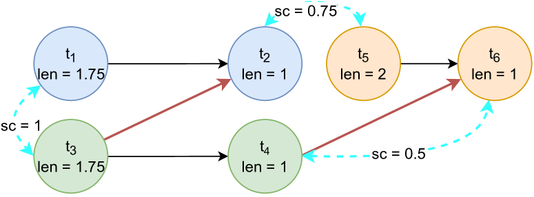
(a) An example DAG. The color of each task represents the owning thread. Red edges denote inter-task dependencies. The blue dashed lines show CPU jumps between tasks belonging to different threads, with the switching cost (sc).

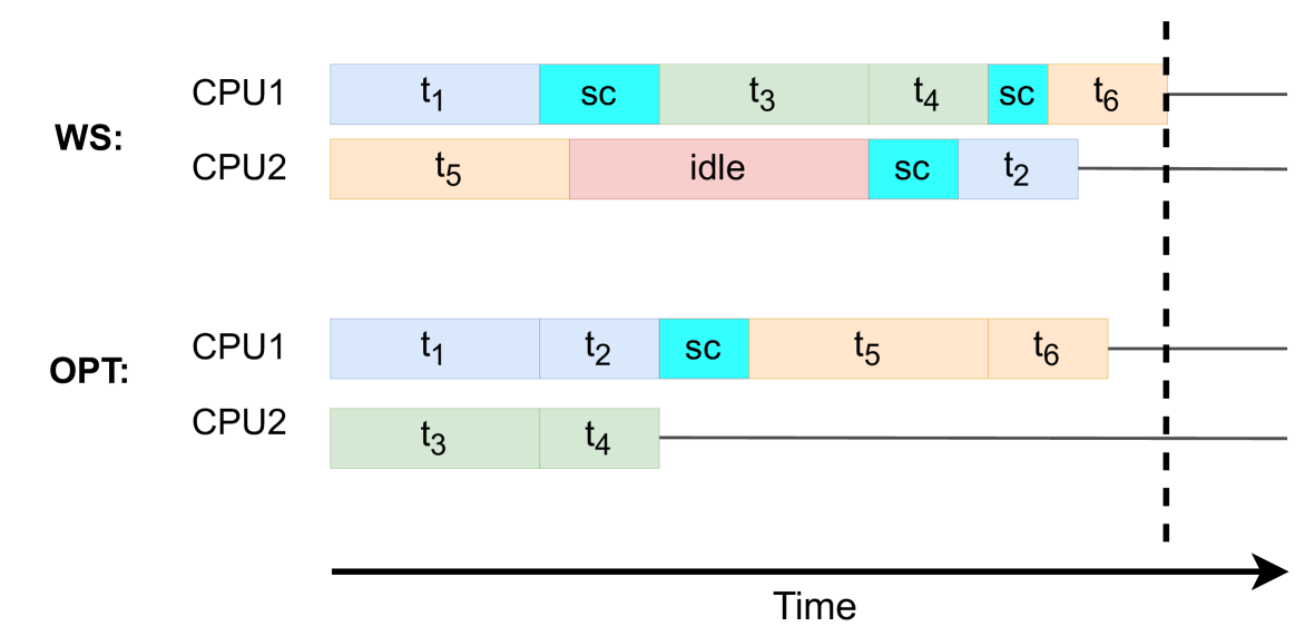
(b) Work Stealing and Optimal schedules

Figure 3: Work Stealing vs Optimal

The solver chooses variables representing two schedules for this job. One schedule is constrained to mimic work stealing and the other can be arbitrary. The solver is instructed to maximize the ratio of the time taken by the work stealing schedule to the time taken to finish the arbitrary one. This forces it to minimize the completion time for the arbitrary schedule, making it optimal. Our queries explore how this ratio varies as we impose different constraints on the context switching costs.

A schedule is represented by the start and finish times for each task, as well as a boolean matrix that maps tasks to CPUs. While the two schedules can be different, constraints ensure that both respect the tasks’ properties, such as their lengths, dependencies, and switching costs. For example, the following constraints ensure that a task is ready to execute when all of its dependencies are finished:

$$\begin{split}&\forall t_{1},t_{2}\in\texttt{tasks}\quad\texttt{edge}(t_{1},t_{2})\implies\\ &t_{1}.\texttt{sched}.\texttt{end\_time}\leq t_{2}.\texttt{sched}.\texttt{ready\_time}\end{split}$$ (1)

$$\begin{split}&\forall t_{2}\in\texttt{tasks}\\ &(\exists t_{1}\in\texttt{tasks},\quad\texttt{edge}(t_{1},t_{2})\quad\land\\ &t_{1}.\texttt{sched}.\texttt{end\_time}=t_{2}.\texttt{sched}.\texttt{ready\_time})\quad\lor\\ &t_{2}.\texttt{sched}.\texttt{ready\_time}=0\end{split}$$ (2)

Fig. 3(b) shows an example work stealing schedule and compares it with the optimal schedule.

5.1 Queries and Results

We ask the solver to maximize the ratio between completion times in the work stealing and unconstrained schedules:

$$\texttt{maximize}(\texttt{time}_{\texttt{ws}}/\texttt{time}_{\texttt{opt}})$$ (3)

First, we set the costs of context switching to zero and queried for the maximal ratio between work stealing and optimal. We found that the bound was not 2, but $2-\frac{1}{P}$, where $P$ is the number of processors. Since we are using an SMT solver, the bound it found is exact and matches the known theoretical result. Thus, even though we only queried for up to 4 processors, 4 threads, and 9 tasks, we believe that the precision and consistency of our results allow for extrapolation to larger values.

Next, we introduce switching costs. We parametrize the switching cost in two ways. Parameter $k$ caps the maximum switching cost and $c$ caps how different the switching costs can be from each other. Formally:

$$\forall t\in\texttt{tasks},\quad\texttt{switch\_cost}(t)\leq k\times\texttt{len}_{\texttt{min}}$$ (4)

$$\begin{split}&\max_{t\in\texttt{tasks}}(\texttt{switch\_cost}(t))\\ &\quad\quad\quad\leq c\times\min_{t\in\texttt{tasks}}(\texttt{switch\_cost}(t))\end{split}$$ (5)

Since the unit of time is arbitrary, we pick one so that the maximum task length is 1. We fix $c=1$ and $k=10$. This means that the solver can select any context switching cost up to $10\times$ the task length, as long as the costs are equal to each other. Figure 4 shows the optimality ratio as we vary the maximum size of the DAG tasks. For small DAGs, work stealing performs close to optimal. The performance worsens linearly as the size increases. It is interesting to note that the bound grows at a slower rate with increasing number of CPUs and the ratio remains bounded even though context switch cost can be up to $10\times$ the task length.

Next, we vary the bound on the maximum allowed switching cost while constraining that all costs be equal to each other. Figure 5 plots the optimality ratio for different numbers of CPUs and tasks. Interestingly, it plateaus to a value only slightly larger than in the case without context switching cost. For instance, with 2 processors and up to 7 tasks, the optimality ratio is smaller than 4.

This sets the stage up for the final result, wherein we we allow switching costs to vary between $0$ and $10$ as long as they are within $c\times$ of each other, as shown in figure 6. Here the ratio grows linearly with $c$, showing that the variation in switching cost matters more than its absolute value.

What can practitioners take away from this analysis? If context switching cost is small, work stealing is near optimal. If not, it is still near optimal if the number of CPUs is large or if cost variation is small and the job is representable by a small DAG. A caveat is that our results are only rigorously proven for small numbers of CPUs and tasks. Nevertheless the numbers fit so perfectly on a line that we are tempted to conjecture and extrapolate.

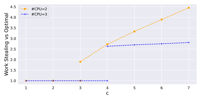
Figure 4: Work Stealing performance for different DAG sizes $(k=10,c=1)$. When the number of tasks is less than the number of CPUs, work stealing is trivially optimal.

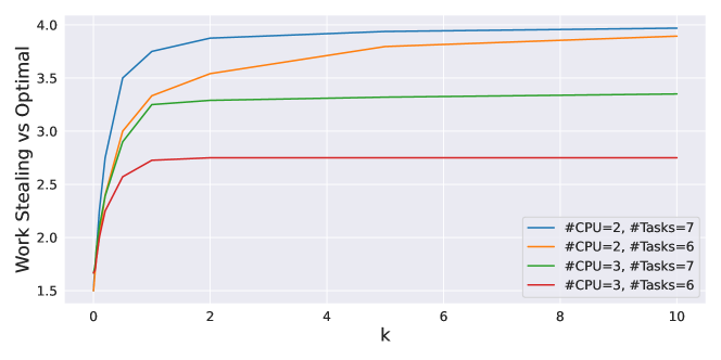
Figure 5: Work Stealing performance as switching costs scale up. Every pair of task has the same cost $(c=1)$.

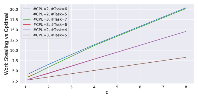
Figure 6: Work Stealing performance when costs between different pairs of tasks can vary. $(k=10)$

6 Case study: The Linux CFS Load Balancer

The Completely Fair Scheduler (CFS) scheduler is the default process scheduler in Linux for systems with multiple processing units. It aims to ensure fairness between running threads without sacrificing performance. We studied the load balancing logic in the CFS scheduler for Linux v5.5 [14].

Overview. The load balancer supports multi-core architectures, including SMT, SMP, and NUMA. To minimize cost, it tries to move tasks between nearby CPUs. To capture how close CPUs are to each other, the load balancer divides CPUs into scheduling domains. Scheduling domains form a hierarchy starting from individual CPUs at bottom level to the top-level domain that includes all CPUs. For example, a domain could be the set of CPUs in the same NUMA node. Ideally, the algorithm should balance load between all CPUs at all domains. However, this task becomes expensive as the number of CPUs grows. To reduce the cost of load balancing, the algorithm balances the aggregate load between groups of CPUs. In particular, each domain is divided into multiple groups, each containing one or more CPUs. The algorithm attempts to balance load between the groups in each domain. Figure 7 shows an example a domain hierarchy.

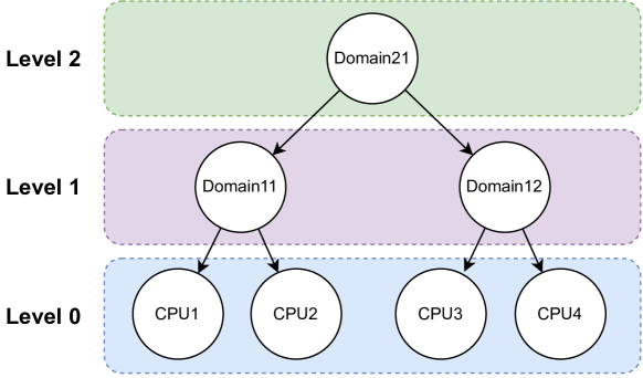
Figure 7: Domain hierarchy with 4 CPUs. The smaller sub-domains also act as the groups of the larger domain.

Algorithm 1 describes LoadBalance(), a function run by CPU c to balance domain sd. Each CPU runs its own instance of the load balancer at regular intervals. At each tick, the balancer traverses the domain hierarchy upwards and calls LoadBalance() to balance work between groups within progressively larger domains. At any point in time, exactly one CPU is responsible to balance the load in a particular domain (Line 36). To avoid moving small tasks between multiple CPUs, the balancer only moves tasks if the imbalance between two groups is larger than a configurable threshold (Line 38). To further reduce the balancing cost, a CPU only moves tasks from the busiest CPU of the busiest group (Line 43). Depending on workload characteristics, the algorithm selects a ‘migration type’ (Line 44). These types define the rules to determine the busiest CPU, the imbalance between two groups, and the load generated by each task. We describe how each decision is made as needed later in the section.

While we attempt to capture the full complexity of the per-tick algorithm, we forego modeling some optional features such as task pinning and priorities. We do not model cache-aware heuristics. Even with these simplifications, we find our model to be expressive enough to discover algorithmic bugs.

Algorithm 1 Linux CFS Load Balancing Algorithm

1:procedure MigrationType($busiest,local,idle$)

2:     if $local.\textrm{HasSpare}()$ then 

3:         if $busiest.\textrm{Overloaded}()$ then

4:              $has\_cap\leftarrow local.capacity>local.util$

5:              if $!idle\textbf{ or }has\_cap$ then

6:                  return MIGRATE_UTIL

7:              else 

8:                  return MIGRATE_TASK                        

9:         $\cdots$      

10:end procedure

11:procedure BusiestCPU($CPUs,m\_type$)

12:     $key1\leftarrow\textbf{lambda}\ c:c.util\_avg$

13:     $key2\leftarrow\textbf{lambda}\ c:c.nr\_running$

14:     $moreThanOne\leftarrow\textrm{Filter}(CPUs,key2)$ $\triangleright$ added in v5.7

15:     switch $m\_type$ do

16:         case MIGRATE_UTIL

17:              return $\textrm{argmax}(moreThanOne,\ key1)$          

18:         case MIGRATE_TASK

19:              return $\textrm{argmax}(CPUs,\ key2)$          

20:         case $\cdots$               

21:end procedure

22:procedure CalcImb($busiest,local,m\_type$)

23:     switch $m\_type$ do

24:         case MIGRATE_UTIL

25:              return $local.capacity-local.util$          

26:         case MIGRATE_TASK

27:              if busiest.Overloaded() then

28:                  return $1$

29:              else

30:                  $t_{1}\leftarrow busiest.nr\_idle$

31:                  $t_{2}\leftarrow local.nr\_idle$

32:                  return $\max(0,(t_{1}-t_{2})/2)$                        

33:         case $\cdots$               

34:end procedure

35:procedure LoadBalance($c,sd$)

36:     if $!\textrm{IsResponsible}(c,sd)$ then

37:         return      

38:     if $!\textrm{ConsiderableImb}(c.idle,sd)$ then

39:         return      

40:     $dst\_g\leftarrow sd.\textrm{FindGroup}(c)$

41:     if $!sd.\textrm{GroupAboveAvg}(dst\_g)$ then

42:         return      

43:     $src\_g\leftarrow sd.\textrm{FindBusiestGroup}()$

44:     $m\_type\leftarrow\textrm{MigrationType}(src\_g,dst\_g,c.idle)$

45:     $src\_c\leftarrow\textrm{BusiestCPU}(src\_g.CPUs,m\_type)$

46:     $imb\leftarrow\textrm{CalcImb}(src\_g,dst\_g,m\_type)$

47:     $\textrm{DetachTasks}(src\_c,c,m\_type,imb)$ $\triangleright$ moves tasks based on migration type

48:end procedure

6.1 Model

At 10,000+ lines of code [17], the load balancer includes several complex heuristics that interact with each other at each scheduling tick to quantify a measure of imbalance, and decide on how to balance it if at all. While we attempt to capture the full complexity of the per-tick algorithm, to keep analysis tractable, we make several simplifications. We forego modeling some optional features such as task pinning and priorities. We also do not model cache-aware heuristics. As a result, our model is sound, but not complete. Nevertheless, our model captures a large subset of possible Linux behaviors and detected several bugs.

In general, CPUs can load balance asynchronously upon becoming idle. However, we choose to only model the per-tick behavior to keep our model tractable. Timesteps are represented as an integer vector of fixed size. Each CPU attempts to balance every domain that it belongs to at fixed, regular intervals between successive timesteps. The domains are balanced in the order of their level in the domain hierarchy.

A task is represented as a collection of real variables to denote properties such as the weighted moving average of the time it was runnable (i.e., runnable average) and its running time (i.e., utilization average). Variables representing the properties of tasks are defined for each timestep. We do not model asynchronous load balancing due to a CPU becoming idle, and assume tasks are runnable through all modeled timesteps. Nevertheless, the solver is free to choose any initial values. For instance, it can pick any initial value of the utilization average and the runnable average of tasks as long as the latter is larger. Since the choice of initial values is unconstrained, this model is akin to simulating a few microseconds starting from any reachable state of the system, including those caused by tasks alternating arbitrarily between runnable and non-runnable.

The domain hierarchy, the number of tasks, and the number of timesteps are configurable parameters. Real valued variables representing CPUs, groups, and domains are also defined for each timestep. For instance, the utilization average of each CPU tracks the sum of utilization averages of each task in its runqueue (i.e., runnable tasks assigned to that CPU). Similarly, a group’s utilization is just the sum of the utilization averages of CPUs contained in it. A CPU $\times$ Task boolean matrix encodes which task is runnin on which CPU at each timestep. Finally, we add constraints that connect metrics and the schedule at successive timesteps, closely following the actual code. As an example, the following constraints represent IsResponsible(c, sd) (line 36), the function that determines if a CPU $c$ is responsible to balance domain $sd$ at timestep $t$:

$$\texttt{first\_idle}(t,c,sd)\lor\texttt{first\_cpu}(t,c,sd)$$

where,

$$\begin{split}&\texttt{first\_idle}(c,sd):=c.\texttt{nr\_running}[t-1]=0\quad\land\\ &\quad\quad\quad\quad(\forall c\textquoteright\in sd,c\textquoteright.\texttt{index}<c.\texttt{index}\implies\\ &\quad\quad\quad\quad\quad\quad c\textquoteright.\texttt{nr\_running}[t-1]>0)\end{split}$$

$$\begin{split}&\texttt{first\_cpu}(c,sd):=c.\texttt{index}=0\quad\land\\ &\quad\quad\quad\quad(\forall c\textquoteright\in sd,c\textquoteright.\texttt{nr\_running}[t-1]>0)\end{split}$$

$c.$nr_running$[t-1]$ is the number of tasks running in CPU $c$ at timestep $t-1$ and $c.$index is a statically assigned index to each CPU. This constraint is applied to every (CPU, domain) pair to find the responsible CPU at each timestep.

6.2 Queries and Verification

For this model, we focus on the Q1 class of questions. In particular, we formulate a single query to verify whether the algorithm is work conservating property of the algorithm. First we set the number of runnable tasks to be greater than the number of CPUs and ask whether at the end of $T$ timesteps, any CPU is idle: $\exists c\in\texttt{CPUs},\quad c.\texttt{nr\_running}[T]==0$

For a work conserving scheduler, the answer should be “no”, no matter how tasks are distributed initially. For small $T$, imbalance is acceptable and sometimes intended by the scheduler to avoid excessive task movement due to sudden changes in workload. We want to detect workloads where it never balances, no matter how long load is imbalanced. We run our model with up to 4 CPUs, 7 tasks, and 6 timesteps. All the bugs discovered with this setup were also found with just 3 timesteps.

6.2.1 Bug 1: Busiest CPU with a single task

As described earlier, there are multiple migration types that are determined based on the state of the system. MIGRATE_UTIL is chosen when the busiest group is overloaded, and the current group has spare capacity (Line 6). Such a decision can be made in the scenario shown in Figure 8 when the utilization average of all tasks in Group 1 is high (e.g. their sum is greater than $90\%$ of the group’s capacity).

Choosing MIGRATE_UTIL implies that the algorithm’s goal is to balance the utilization average amongst groups by stealing tasks from the busiest CPU. The CPU with the highest utilization average in the busiest group is determined to be the busiest (Line 17). A CPU’s utilization average is just the sum of utilization averages of the tasks in its runqueue. The utilization average of a task is defined as the weighted moving average of its running time in the past.

In our example, CPU2 can be the busiest CPU, even though it has a single task, if that task has a higher utilization average than the sum of the utilization averages of tasks on CPU1. However CPU3 steal work from CPU2 since it only has a single runnable task. This constraint helps avoid bouncing tasks between idle CPUs, but causes the scheduler to not be work conserving. One way to fix this ‘bug’ is to define the busiest CPU to be the one with the highest utilization average that has more than one runnable task (line 14). After finding the bug using this model, we realized that it was also identified by the Linux community and fixed in Linux v5.7 [16] .

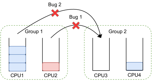
Figure 8: Example state to showcase the bugs. Except CPU3, each CPU’s runqueue has tasks represented as rectangles. CPU3 is idle. Under different settings, CPU3 may be unable to steal any task from Group 1.

6.2.2 Bug 2: Imbalance with idle CPUs

With the previous bug fixed, we reran the work conservation query, identifying another bug. This bug happens when the migration type ‘MIGRATE_TASK’ is selected. Task migration is chosen when the the current group has spare capacity, but the conditions for the type ‘MIGRATE_UTIL‘ are not satisfied. In particular, it can be selected when no group is overloaded. Here, the algorithm’s goal is to balance the number of tasks between groups. The busiest CPU in the busiest group is decided based on the number of tasks in the runqueue of the CPU. Imbalance is defined as half of the difference between the number of idle CPUs in the busiest and the current group (Line 32). At first glance, this seems reasonable and should even out the number of idle CPUs. However, Linux can only perform integer division, leading to calculating the imbalance to be zero when the difference in idle CPUs is 1. This behavior is captured by the scenario in Figure 8 when group 1 is not overloaded. CPU1 is deemed as the busiest CPU with 3 tasks, but CPU3 is still unable to steal any of them.

It is worth noting that both these issues intricately depend on the workload characteristics generated by our solver. Slight deviation in these characteristics can lead to a completely different outcome. For instance, a different migration type may apply as the number of tasks or the blocking pattern of existing tasks evolves. A different measure of imbalance may be able to push tasks to idle CPUs and balance load more evenly in general. Finely controlling the workload characteristics in synthetic benchmarks that highlight these bugs is difficult. This makes it hard for fuzzers and other tests to detect them. However, it does not preclude them from appearing in the real world. Our framework is not limited by this, and can freely search the workload space to generate intricate violating traces.

7 Case study: TCP Synchronization in Ring Allreduce Training

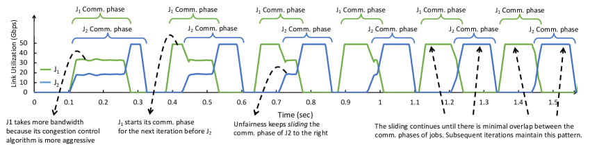
Figure 9: Intuition behind why synchronization occurs. Reproduced from [37] with permission.

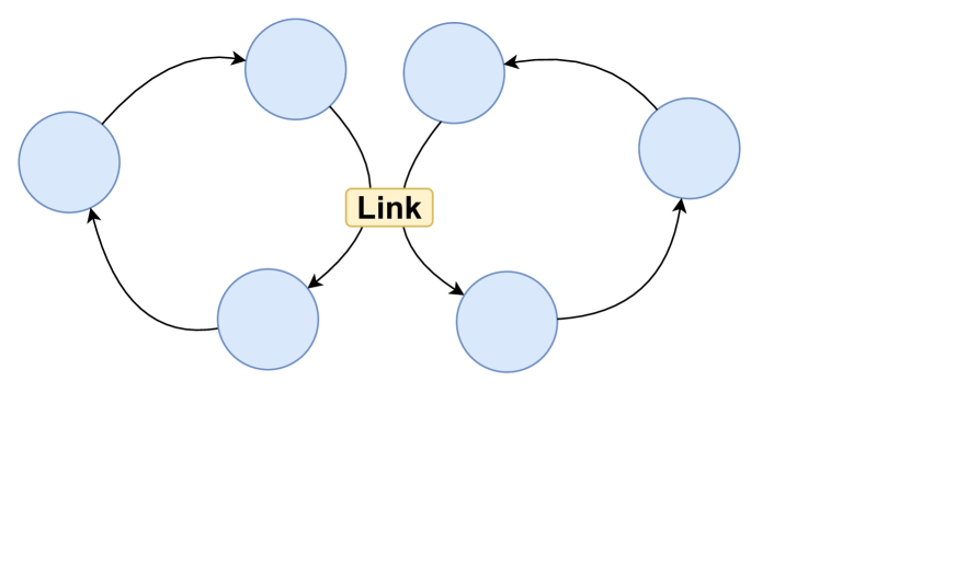
(a)

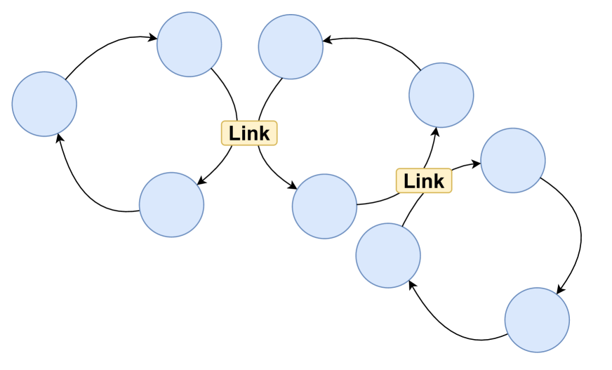
(b)

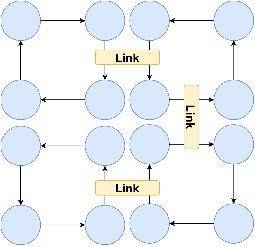
(c)

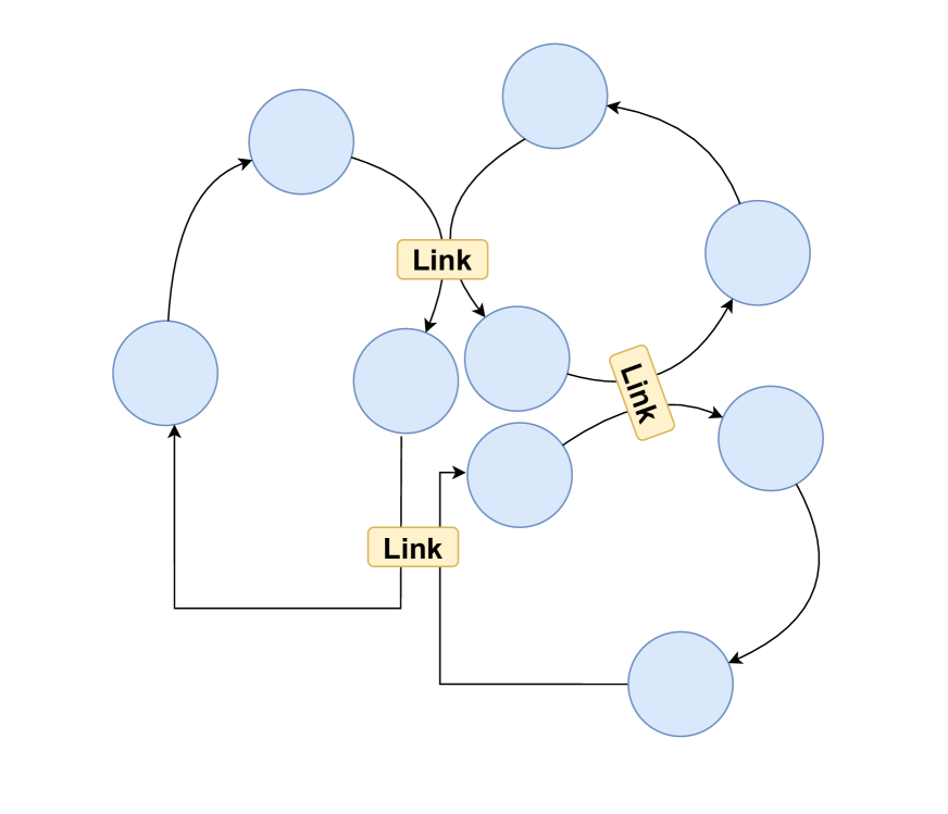
(d)

Figure 10: Configurations of ring reduce jobs sharing links

The above examples look at well-known schedulers. Perhaps the most compelling use-case for our methodology is to understand less well-studied systems. As an example, we considered a recent paper [37] which examines complex emergent behavior in a cluster running multiple distributed neural network training jobs. Neural network training processes data in batches, computing the gradient of the error function for each batch to adjust the weights before processing the next batch. The computation-communication pattern for each batch is similar, making the process predictable and providing opportunities for better scheduling [35, 46, 43].

A training job consists of $n$ servers connected logically in a ring. During training, servers have phases involving intense computation followed by communication along the ring. A datacenter may run multiple jobs sharing the same physical network. As a result, some of the logical links may be shared with other training jobs as shown in figure 10. One can maximize network utilization by scheduling one job’s computation while the other communicates. This way, each job gets the full available bandwidth to itself when it is communicating. The reference paper [37] observes that jobs spontaneously synchronize to this desired schedule due to TCP unfairness. In this section, we verify this claim under complex settings and find it to be true.

Preliminaries: We provide a brief overview of data-parallel distributed training using the ring-all-reduce method, omitting details that are not necessary to understand the scheduling problem. Each round of training processes one batch and consists of three phases: backpropagation, sum and broadcast. The first is purely computation and the rest are primarily communication. The model is divided into $n$ pieces. Servers transmit data as soon as it is available. When summing, the first piece is available as soon as backpropagation is done processing that part of the neural network. After this the server must wait for data from the preceeding server before forwarding it. The same holds for the broadcast step, except that the first piece is immediately available.

Figure 9 is an experimental result showing the intuition behind why synchronization occurs. Suppose job 1 has been transmitting on the shared link at full link capacity, and a new job 2 starts transmitting over the same link. Both jobs will detect the congestion and adjust their sending rates so that both transmit at half of the full link capacity. However, it takes time for the transmission rates to reach this new equilibrium and many congestion control algorithms never reach it. In the meantime, job 1 gets more bandwidth than flow 2. As a result, the job corresponding to flow 1 will finish its sum and broadcast steps earlier than it otherwise would have, which will make it start even sooner for the next batch. This will continue until the transmissions on the shared link are fully separated in time – which is what we ideally want.

This argument works for when there are just two rings. But what if there are more? One shared link could be forcing the job to slowly its schedule in one direction, while another shared link has an opposite effect. There could even be cycles. Figure 10 illustrates representative examples of the topologies for which we verify synchronization.

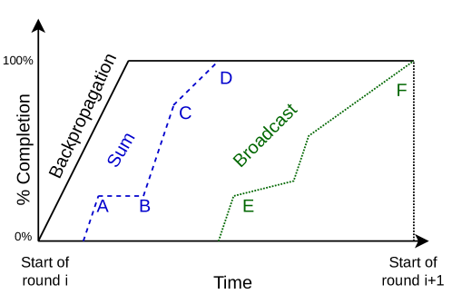
Figure 11: Example of one server’s view of ring reduce during one round. Point A shows that server can send the first $1/n^{th}$ chunk of data as soon as it has computed the gradients for that segment of the network. Till point B, it is waiting for the previous server to send data. Between B to C, it is sending at link rate. Between C and D, it is sharing the link with another job, due to which it sends at a lower rate. Once sum finishes, broadcast can start. Again, the first chunk can be sent without waiting for data from the previous server (point E). After this, it sends at less than line rate because it is waiting on data from the previous server, which it forwards as soon as possible.

Figure 11 shows some model variables for a single server at each timestep. These include the percentage of backpropagation, sum, and broadcast finished. It also includes an integer indicating the round number. A round is defined as the processing of a batch. We keep the state transition function between timesteps simple. For example, the number of flows transmitting on any link is fixed between two timesteps. However, the time gap between timesteps is variable, allowing the solver to add a timestep whenever this changes. This way, we do not discretize time.

In several places, we overapproximate. For example, we do not model the congestion control algorithm explicitly, but instead, constrain that (1) the link is fully utilized and (2) whichever job starts transmitting first gets more bandwidth. This models a wide range of congestion control behaviors while keeping the reasoning simple for both computers and humans. Additionally, we allow a server to send the first $1/n^{th}$ chunk of "sum" and "broadcast" data as soon as it is done computing, without waiting for data from its predecessor. The amount of data it can send depends on the neural network architecture and system structure. Hence we let the solver arbitrarily pick the how much data is available.

To verify synchronization, we constrain that the communication of each job can fit inside the computation time of its neighbors, which is the only case in which the results in our reference paper hold. We then ask the solver to find a case where overlap in communication increases (or remains constant). If the solver cannot find such a case, we have proved that synchronization will always occur. It is important to note that the solver only proves this for a small and finite number of events, and the initial state is unconstrained. However, this also proves that a larger sequence of events cannot exist where communication overlap increases, as if such a sequence were to exist, there would be a short sub-sequence where it increases, which we have proved is impossible.

8 Related Work

Automated Verification. A long history of automated verification of schedulers can be traced back to mechanized proofs of real-time scheduling algorithms using proof assistants like Coq. These include proofs for specific algorithms such as Priority Inheritance [45], implementations in systems like CertiKOS [21], and frameworks to design them [8, 28]. These focus on qualitative correctness properties such as ensuring no task misses a deadline. In contrast, we focus on verifying quantitative performance properties and optimality. In a similar vein, model checking has achieved incredible success in formally verifying large scale systems including network stacks [33, 36, 41], language runtimes [23, 25], and databases [20]. Large parts of the Linux subsystems have also been verified [42, 19]. Our approach has been directly inspired from model checking principles of building abstract models with specifications to verify it. However, existing model checking tools are restricted to identifying correctness bugs. We provide a framework to apply these principles to identify subtle performance bugs in schedulers.

The verification work closest to our approach is CCAC [2]. CCAC models congestion control algorithms to formally verify their performance or generate violating traces. While CCAC provides a specialized tool for modeling congestion control algorithms, our framework is general and is applicable to a larger class of scheduling algorithms.

Tracing and Benchmarking. All major operating systems include specialized tracers to analyze kernel performance. ftrace and perf_events are tracers built into Linux. They provide hooks to instrument various subsystems including the scheduler, and generate performance statistics. More recently, eBPF [39] and SystemTap [38] extend this functionality by allowing custom user code to run inside the kernel to detect specific behavior. These tracers are used in conjunction with standard benchmark suites to detect performance issues. Hackbench [13] benchmarks the average latency for communication between tasks, and has become the defacto standard to test improvements on the Linux load balancer. While tracers and benchmarks are often useful in detecting and explaining unexpected performance behavior, they provide no guarantees on absence of bugs. Our framework, on the other hand, is an attempt to provide formal guarantees on scheduler performance.

9 Limitations and Conclusion

While we believe our methodology to be generally applicable to all scheduling algorithms, it is not a panacea for detecting all problems in an algorithm. Our methodology is dependent on the user’s ingenuity in creating tractable models and formulating relevant queries. For example, our model of the Linux CFS load balancer included several simplifying assumptions (e.g., ignoring asynchronous load balancing steps), yet the model was useful enough to detect practical bugs. Further, our modeling approach can only find performance issues for which a user formulates a metric and query; deeper issues which are not exposed by user–generated queries are not detected by our approach. Solver performance limitations mean that we can only perform bounded model checking, so our models won’t detect problems that happen only in the presence of large number of tasks or events. However, we find that in many scenarios, it’s possible to generalize our results by creating models that focus on critical system components and formulating reasonable queries.

In conclusion, we have demonstrated that formal methods can provide a deeper and more rigorous understanding of scheduling heuristics used in practice. Further, since we verify the specification of these heuristics, and not the code, verification effort is minimal. The most time consuming part of our method is posing the right queries and interpreting counterexamples in context. We invite the community to adopt quantitaive verification as a part of their worklflow when developing scheduling heuristics.

References

- [1] Stefan Andrei, Albert M. K. Cheng, Vlad Radulescu, Sharfuddin Alam, and Suresh Vadlakonda. A new scheduling algorithm for non-preemptive independent tasks on a multi-processor platform. SIGBED Rev., 13(2):24–29, apr 2016.
- [2] Venkat Arun, Mina Tahmasbi Arashloo, Ahmed Saeed, Mohammad Alizadeh, and Hari Balakrishnan. Toward formally verifying congestion control behavior. In Proceedings of the 2021 ACM SIGCOMM 2021 Conference, SIGCOMM ’21, page 1–16, New York, NY, USA, 2021. Association for Computing Machinery.
- [3] Nikhil Bansal and David Gamarnik. Handling load with less stress. Queueing Systems, 54:45–54, 2006.
- [4] Nikhil Bansal and Mor Harchol-Balter. Analysis of SRPT scheduling: Investigating unfairness. In Proceedings of the 2001 ACM SIGMETRICS International Conference on Measurement and Modeling of Computer Systems, SIGMETRICS ’01, page 279–290, New York, NY, USA, 2001. Association for Computing Machinery.
- [5] Ryan Beckett, Aarti Gupta, Ratul Mahajan, and David Walker. A general approach to network configuration verification. In Proceedings of the Conference of the ACM Special Interest Group on Data Communication, SIGCOMM ’17, page 155–168, New York, NY, USA, 2017. Association for Computing Machinery.
- [6] Robert D. Blumofe and Charles E. Leiserson. Scheduling multithreaded computations by work stealing. J. ACM, 46(5):720–748, sep 1999.
- [7] James Bornholt, Rajeev Joshi, Vytautas Astrauskas, Brendan Cully, Bernhard Kragl, Seth Markle, Kyle Sauri, Drew Schleit, Grant Slatton, Serdar Tasiran, Jacob Van Geffen, and Andrew Warfield. Using lightweight formal methods to validate a key-value storage node in amazon s3. In Proceedings of the ACM SIGOPS 28th Symposium on Operating Systems Principles, SOSP ’21, page 836–850, New York, NY, USA, 2021. Association for Computing Machinery.
- [8] Felipe Cerqueira, Felix Stutz, and Björn B. Brandenburg. Prosa: A case for readable mechanized schedulability analysis. In 2016 28th Euromicro Conference on Real-Time Systems (ECRTS), pages 273–284, 2016.
- [9] Tej Chajed, Joseph Tassarotti, M. Frans Kaashoek, and Nickolai Zeldovich. Verifying concurrent, crash-safe systems with perennial. In Proceedings of the 27th ACM Symposium on Operating Systems Principles, SOSP ’19, page 243–258, New York, NY, USA, 2019. Association for Computing Machinery.
- [10] Leonardo Mendonça de Moura and Nikolaj S. Bjørner. Z3: an efficient SMT solver. In Tools and Algorithms for the Construction and Analysis of Systems, 14th International Conference, TACAS, pages 337–340, 2008.
- [11] Seyed K. Fayaz, Tushar Sharma, Ari Fogel, Ratul Mahajan, Todd Millstein, Vyas Sekar, and George Varghese. Efficient network reachability analysis using a succinct control plane representation. In Proceedings of the 12th USENIX Conference on Operating Systems Design and Implementation, OSDI’16, page 217–232, USA, 2016. USENIX Association.
- [12] Ari Fogel, Stanley Fung, Luis Pedrosa, Meg Walraed-Sullivan, Ramesh Govindan, Ratul Mahajan, and Todd Millstein. A general approach to network configuration analysis. In Proceedings of the 12th USENIX Conference on Networked Systems Design and Implementation, NSDI’15, page 469–483, USA, 2015. USENIX Association.
- [13] The Linux Foundation. Hackbench. https://wiki.linuxfoundation.org/realtime/documentation/howto/tools/hackbench.
- [14] The Linux Foundation. Linux Kernel v5.5. https://elixir.bootlin.com/linux/v5.5-rc2/source, 2020.
- [15] The Linux Foundation. Linux Kernel v5.5 Load Balancer lore. https://lore.kernel.org/lkml/1571405198-27570-1-git-send-email-vincent.guittot@linaro.org/, 2020.
- [16] The Linux Foundation. Linux Kernel v5.7 Load Balancer commit fix. https://github.com/torvalds/linux/commit/c32b4308295aaaaedd5beae56cb42e205ae63e58, 2020.
- [17] The Linux Foundation. Linux Load Balancer sched/fair.c. https://elixir.bootlin.com/linux/v5.5.19/source/kernel/sched/fair.c, 2020.
- [18] Joshua Fried, Zhenyuan Ruan, Amy Ousterhout, and Adam Belay. Caladan: Mitigating interference at microsecond timescales. In Proceedings of the 14th USENIX Conference on Operating Systems Design and Implementation, OSDI’20, USA, 2020. USENIX Association.
- [19] Andy Galloway, Gerald Lüttgen, Jan Tobias Mühlberg, and Radu I. Siminiceanu. Model-checking the linux virtual file system. In Neil D. Jones and Markus Müller-Olm, editors, Verification, Model Checking, and Abstract Interpretation, pages 74–88, Berlin, Heidelberg, 2009. Springer Berlin Heidelberg.
- [20] Milos Gligoric and Rupak Majumdar. Model checking database applications. In Proceedings of the 19th International Conference on Tools and Algorithms for the Construction and Analysis of Systems, TACAS’13, page 549–564, Berlin, Heidelberg, 2013. Springer-Verlag.
- [21] Xiaojie Guo, Maxime Lesourd, Mengqi Liu, Lionel Rieg, and Zhong Shao. Integrating formal schedulability analysis into a verified os kernel. In Isil Dillig and Serdar Tasiran, editors, Computer Aided Verification, pages 496–514. Springer International Publishing, 2019.
- [22] Travis Hance, Andrea Lattuada, Chris Hawblitzel, Jon Howell, Rob Johnson, and Bryan Parno. Storage systems are distributed systems (so verify them that way!). In Proceedings of the 14th USENIX Conference on Operating Systems Design and Implementation, OSDI’20, USA, 2020. USENIX Association.
- [23] Thomas A. Henzinger, Ranjit Jhala, Rupak Majumdar, and Grégoire Sutre. Software verification with blast. In Thomas Ball and Sriram K. Rajamani, editors, Model Checking Software, pages 235–239, Berlin, Heidelberg, 2003. Springer Berlin Heidelberg.
- [24] Jeehoon Kang, Yoonseung Kim, Youngju Song, Juneyoung Lee, Sanghoon Park, Mark Dongyeon Shin, Yonghyun Kim, Sungkeun Cho, Joonwon Choi, Chung-Kil Hur, and Kwangkeun Yi. Crellvm: Verified credible compilation for llvm. In Proceedings of the 39th ACM SIGPLAN Conference on Programming Language Design and Implementation, PLDI 2018, page 631–645, New York, NY, USA, 2018. Association for Computing Machinery.
- [25] Daniel Kroening and Michael Tautschnig. Cbmc – c bounded model checker. In Erika Ábrahám and Klaus Havelund, editors, Tools and Algorithms for the Construction and Analysis of Systems, pages 389–391, Berlin, Heidelberg, 2014. Springer Berlin Heidelberg.
- [26] Xavier Leroy. Formal verification of a realistic compiler. Commun. ACM, 52(7):107–115, jul 2009.
- [27] Jed Liu, William Hallahan, Cole Schlesinger, Milad Sharif, Jeongkeun Lee, Robert Soulé, Han Wang, Călin Caşcaval, Nick McKeown, and Nate Foster. P4v: Practical verification for programmable data planes. In Proceedings of the 2018 Conference of the ACM Special Interest Group on data communication, pages 490–503, 2018.
- [28] Mengqi Liu, Lionel Rieg, Zhong Shao, Ronghui Gu, David Costanzo, Jung-Eun Kim, and Man-Ki Yoon. Virtual timeline: A formal abstraction for verifying preemptive schedulers with temporal isolation. Proc. ACM Program. Lang., 4(POPL), dec 2019.
- [29] Nuno P. Lopes, Juneyoung Lee, Chung-Kil Hur, Zhengyang Liu, and John Regehr. Alive2: Bounded translation validation for llvm. In Proceedings of the 42nd ACM SIGPLAN International Conference on Programming Language Design and Implementation, PLDI 2021, page 65–79, New York, NY, USA, 2021. Association for Computing Machinery.
- [30] Nuno P. Lopes, David Menendez, Santosh Nagarakatte, and John Regehr. Practical verification of peephole optimizations with alive. Commun. ACM, 61(2):84–91, jan 2018.
- [31] Jean-Pierre Lozi, Baptiste Lepers, Justin Funston, Fabien Gaud, Vivien Quéma, and Alexandra Fedorova. The linux scheduler: A decade of wasted cores. In Proceedings of the Eleventh European Conference on Computer Systems, EuroSys ’16, New York, NY, USA, 2016. Association for Computing Machinery.
- [32] Sarah McClure, Amy Ousterhout, Scott Shenker, and Sylvia Ratnasamy. Efficient scheduling policies for Microsecond-Scale tasks. In 19th USENIX Symposium on Networked Systems Design and Implementation (NSDI 22), pages 1–18, Renton, WA, April 2022. USENIX Association.
- [33] Madanlal Musuvathi and Dawson R. Engler. Model checking large network protocol implementations. In Proceedings of the 1st Conference on Symposium on Networked Systems Design and Implementation - Volume 1, NSDI’04, page 12, USA, 2004. USENIX Association.
- [34] Amy Ousterhout, Joshua Fried, Jonathan Behrens, Adam Belay, and Hari Balakrishnan. Shenango: Achieving high cpu efficiency for latency-sensitive datacenter workloads. In Proceedings of the 16th USENIX Conference on Networked Systems Design and Implementation, NSDI’19, page 361–377, USA, 2019. USENIX Association.
- [35] Yanghua Peng, Yibo Zhu, Yangrui Chen, Yixin Bao, Bairen Yi, Chang Lan, Chuan Wu, and Chuanxiong Guo. A generic communication scheduler for distributed dnn training acceleration. In Proceedings of the 27th ACM Symposium on Operating Systems Principles, SOSP ’19, page 16–29, New York, NY, USA, 2019. Association for Computing Machinery.
- [36] Santhosh Prabhu, Kuan-Yen Chou, Ali Kheradmand, P. Brighten Godfrey, and Matthew Caesar. Plankton: Scalable network configuration verification through model checking. In Proceedings of the 17th Usenix Conference on Networked Systems Design and Implementation, NSDI’20, page 953–968, USA, 2020. USENIX Association.
- [37] Sudarsanan Rajasekaran, Manya Ghobadi, Gautam Kumar, and Aditya Akella. Congestion control in machine learning clusters. ACM HotNets 2022, 2022.
- [38] Red Hat. SystemTap. https://sourceware.org/systemtap/, 2005.
- [39] Alastair Robertson. bpftrace: High-level tracing language for Linux eBPF. https://github.com/iovisor/bpftrace, 2019.
- [40] Linus Schrage and Louis Miller. The queue M/G/1 with the shortest remaining processing time discipline. Operations Research, 14(4):670–684, 1966.
- [41] Wei Sun, Lisong Xu, Sebastian Elbaum, and Di Zhao. Model-agnostic and efficient exploration of numerical state space of real-world tcp congestion control implementations. In Proceedings of the 16th USENIX Conference on Networked Systems Design and Implementation, NSDI’19, page 719–733, USA, 2019. USENIX Association.
- [42] Thomas Witkowski, Nicolas Blanc, Daniel Kroening, and Georg Weissenbacher. Model checking concurrent linux device drivers. In Proceedings of the Twenty-Second IEEE/ACM International Conference on Automated Software Engineering, ASE ’07, page 501–504, New York, NY, USA, 2007. Association for Computing Machinery.
- [43] Wencong Xiao, Romil Bhardwaj, Ramachandran Ramjee, Muthian Sivathanu, Nipun Kwatra, Zhenhua Han, Pratyush Patel, Xuan Peng, Hanyu Zhao, Quanlu Zhang, Fan Yang, and Lidong Zhou. Gandiva: Introspective cluster scheduling for deep learning. In 13th USENIX Symposium on Operating Systems Design and Implementation (OSDI 18), pages 595–610, Carlsbad, CA, October 2018. USENIX Association.
- [44] Irene Zhang, Amanda Raybuck, Pratyush Patel, Kirk Olynyk, Jacob Nelson, Omar S. Navarro Leija, Ashlie Martinez, Jing Liu, Anna Kornfeld Simpson, Sujay Jayakar, Pedro Henrique Penna, Max Demoulin, Piali Choudhury, and Anirudh Badam. The demikernel datapath os architecture for microsecond-scale datacenter systems. In Proceedings of the ACM SIGOPS 28th Symposium on Operating Systems Principles, SOSP ’21, page 195–211, New York, NY, USA, 2021. Association for Computing Machinery.
- [45] Xingyuan Zhang, Christian Urban, and Chunhan Wu. Priority inheritance protocol proved correct. J. Autom. Reason., 64(1):73–95, jan 2020.
- [46] Yihao Zhao, Yuanqiang Liu, Yanghua Peng, Yibo Zhu, Xuanzhe Liu, and Xin Jin. Multi-resource interleaving for deep learning training. In Proceedings of the ACM SIGCOMM 2022 Conference, SIGCOMM ’22, page 428–440, New York, NY, USA, 2022. Association for Computing Machinery.