New Exact Betchov-like Relation for the Helicity Flux in Homogeneous Turbulence

Abstract

In homogeneous and isotropic turbulence, the relative contributions of different physical mechanisms to the energy cascade can be quantified by an exact decomposition of the energy flux (P. Johnson, Phys. Rev. Lett., 124, 104501 (2020), J. Fluid Mech. 922, A3(2021)). We extend the formalism to the transfer of kinetic helicity across scales, important in the presence of large-scale mirror breaking mechanisms, to identify physical processes resulting in helicity transfer and quantify their contributions to the mean flux in the inertial range. All subfluxes transfer helicity from large to small scales. About 50$\%$ of the mean flux is due to the scale-local vortex flattening and vortex twisting. We derive a new exact relation between these effects, similar to the Betchov relation for the energy flux, revealing that the mean contribution of the former is three times larger than that of the latter. Multi-scale effects account for the remaining 50$\%$ of the mean flux, with approximate equipartition between multi-scale vortex flattening, twisting and entangling.

1 Introduction

The kinetic helicity, defined as the $L^{2}$-inner product of velocity $\bm{u}$ and vorticity $\bm{\omega}$, has dynamical, topological, geometrical, and statistical interpretations in turbulence. It is a dynamical and topological inviscid invariant, where the latter refers to its connection with the linking number of infinitesimal vortex lines (Moffatt, 1969). Geometrically, it quantifies the alignment of velocity and vorticity in a volume-averaged sense. Within a statistical approach to turbulence, helicity is the correlation between velocity and vorticity. In a rotationally invariant ensemble, it is connected to the breaking of the symmetry under inversion of all axes. Inspired by its relevance to turbulence in atmospheric flows (Lilly, 1986), dynamical and statistical effects connected with helicity have been studied in the atmospheric boundary layer (Deusebio & Lindborg, 2014) and in rotating turbulence (Mininni & Pouquet, 2010a, b), and more generally in homogeneous and isotropic turbulence (Chen et al., 2003a, b; Gledzer & Chkhetiani, 2015; Kessar et al., 2015; Sahoo et al., 2015; Stepanov et al., 2015; Alexakis, 2017; Sahoo et al., 2017; Milanese et al., 2021; Yan et al., 2020), as well as shear flows (Yan et al., 2020; Yu et al., 2022) and in laboratory experiments (Scheeler et al., 2017).

The level of helicity in a turbulent flow affects turbulent statistics and dynamics, and is thus of relevance from a fundamental theory perspective as well as for subgrid-scale (SGS) modelling. As an alignment of velocity and vorticity weakens the nonlinearity of the Navier–Stokes equations, high levels of helicity have been connected with a depletion of the kinetic energy flux across scales by an analysis of the coupling between helical Fourier modes (Kraichnan, 1973), and with regions of low dissipation (Moffatt, 2014). These effects can be quantified by upper bound theory applied to helical forcing and direct numerical simulation — the energy flux of turbulence sustained by fully helical forcing is about $30\%$ lower than in the non-helical case (Linkmann, 2018).

Helicity affects turbulence not only globally, that is, in terms of mean energy fluxes, but also on a scale-by-scale level. As a solenoidal vector field, the velocity field $\bm{u}$ can be decomposed into positively and negatively helical components $\bm{u}^{\pm}$ (Herring, 1974; Constantin & Majda, 1988; Waleffe, 1992), $\bm{u}(\bm{x},t)=\bm{u}^{+}(\bm{x},t)+\bm{u}^{-}(\bm{x},t)$, where $\bm{u}^{\pm}$ are obtained by projecting the Fourier coefficients $\hat{\bm{u}}(\bm{k},t)$ onto basis vectors which are eigenfunctions of the curl operator in Fourier space. That is, $\hat{\bm{u}}^{\pm}(\bm{k},t)=u^{\pm}(\bm{k},t)\bm{h}^{\pm}(\bm{k})\ ,$ where $i\bm{k}\times k\bm{h}^{\pm}(\bm{k})=\pm\bm{h}^{\pm}(\bm{k})$ and $u^{\pm}(\bm{k},t)=\hat{\bm{u}}(\bm{k},t)\cdot\bm{h}^{\pm}(\bm{k})$. The energy flux can then be decomposed into different triadic couplings between positively and negatively helical velocity-field fluctuations (Waleffe, 1992). Interestingly, interactions among helical Fourier modes of like-signed helicity leads to an inverse energy transfer across scales in the inertial range (Waleffe, 1992; Biferale et al., 2012, 2013; Sahoo et al., 2015), while interactions of oppositely-signed helical modes transfer energy from large to small scales (Waleffe, 1992; Alexakis, 2017; Alexakis & Biferale, 2018). For turbulent flows of electrically conducting fluids such as liquid metals or plasmas in the fluid approximation, helicity alters the evolution of both velocity and magnetic-field fluctuations profoundly. Here, small-scale kinetic helicity facilitates the formation of large-scale coherent magnetic structures through the large-scale dynamo (Steenbeck et al., 1966; Brandenburg, 2001; Brandenburg & Subramanian, 2005; Tobias et al., 2013; Linkmann et al., 2016, 2017).

The cascade of kinetic helicity itself is predicted to be direct, that is, it proceeds from large to small scales (Brissaud et al., 1973; Waleffe, 1992), and scale-local (Eyink, 2005). It results, as discussed by Eyink (2006) in the context of a multi-scale gradient expansion, from a twisting of small-scale vortices into a local alignment with the small-scale velocity fluctuations by large-scale differential vorticity (‘screw’). However, being sign-indefinite, numerical results on helicity fluxes can be difficult to interpret as a loss of positive helicity at a given scale may be viewed as a gain of negative helicity at the same scale.

In the context of SGS modelling, the effect helicity has on a turbulent flow is usually taken into account though additional diffusive model terms (Yokoi & Yoshizawa, 1993; Li et al., 2006; Baerenzung et al., 2008; Inagaki et al., 2017). However, a combination of a-priori and a-posteriori analyses of different SGS models for isotropic helical turbulence found the effect of the additional diffusive model terms to be small and that a classical Smagorinsky model best represents the resolved-scale dynamics (Li et al., 2006). Similarly, based on analytical and numerical results, Linkmann (2018) suggests an adjustment of the Smagorinsky constant to account for high levels of helicity. So far, SGS analyses of helical turbulence have mainly been concerned with energy transfers.

Here, we focus on the helicity flux across scales in statistically stationary homogeneous and isotropic turbulence, with large-scale forcing breaking mirror symmetry. For the energy flux, the Betchov (1956) relation states that the mean contribution from vortex stretching to the energy cascade is triple that due to strain self-amplification. Carbone & Wilczek (2022) recently showed that there are no further kinematic relations for the energy flux in statistically stationary homogeneous and isotropic turbulence with zero net helicity. However, we prove here that a new exact kinematic Betchov-type relation exists for the mean helicity flux. Furthermore, we also present an exact decomposition of the helicity flux in analogy to that of the kinetic energy flux derived by Johnson (2020, 2021), whereby the relative contributions of physical mechanisms, such as vortex stretching and strain self-amplification, to the energy cascade can be quantified in terms of the overall contribution and their scale-locality. The aim is to identify physical mechanisms that transfer kinetic helicity across scales and to quantify their relative contributions to the mean helicity flux and its fluctuations, which may be useful for the construction of SGS models when resolving the helicity cascade is of interest.

2 Exact decomposition of the kinetic helicity flux

To derive the aforementioned exact decomposition of the helicity flux and relations between the resulting subfluxes, we begin with the three-dimensional (3D) incompressible Navier–Stokes equations, here written in component form

$$\partial_{t}u_{i}+\partial_{j}\left(u_{i}u_{j}\right) =-\partial_{j}p\delta_{ij}+2\nu\partial_{j}S_{ij}+f_{i}\ ,$$ (1)

$$\partial_{j}u_{j} =0\ ,$$ (2)

where $\bm{u}=(u_{1},u_{2},u_{3})$ is the velocity field, $p$ the pressure divided by the constant density, $\nu$ the kinematic viscosity, $S_{ij}$ the rate-of-strain tensor, and $\bm{f}=(f_{1},f_{2},f_{3})$ an external solenoidal force that may be present. To define the helicity flux across scales, we introduce a filtering operation to separate large- and small-scale dynamics (e.g., Germano, 1992). Specifically, for a generic function $\phi$, the filtered version at scale $\ell$ is $\overline{\phi}^{\ell}=G^{\ell}*\phi\ ,$ where $G^{\ell}$ is a filter kernel with filter width $\ell$ and the asterisk denotes the convolution operation. Applying the filter to the Navier–Stokes equations (1)–(2) results in

$$\partial_{t}\overline{u}^{\ell}_{i}+\partial_{j}\left(\overline{u}^{\ell}_{i}\overline{u}^{\ell}_{j}+\overline{p}^{\ell}\delta_{ij}-2\nu\overline{S}^{\ell}_{ij}+\tau_{ij}^{\ell}\right)=\overline{f}_{i}^{\ell}\ ,$$ (3)

where $\tau_{ij}^{\ell}=\tau^{\ell}(u_{i},u_{j})=\overline{u_{i}u_{j}}^{\ell}-\overline{u}^{\ell}_{i}\overline{u}^{\ell}_{j}$ is the SGS stress tensor. Here, we follow the notation of Germano (1992) in defining the generalised second moment for any two fields as $\tau^{\ell}(a,b)=\overline{ab}^{\ell}-\overline{a}^{\ell}\overline{b}^{\ell}$. We also require the filtered vorticity equation

$$\partial_{t}\overline{\omega}^{\ell}_{i}+\partial_{j}\left(\overline{\omega}^{\ell}_{i}\overline{u}^{\ell}_{j}-\overline{u}^{\ell}_{i}\overline{\omega}^{\ell}_{j}-\nu\partial_{j}\overline{\omega}^{\ell}_{i}\right)-\overline{g}_{i}^{\ell}=-\partial_{j}\left(\epsilon_{imn}\partial_{m}\tau^{\ell}_{nj}\right)\ ,$$ (4)

where $\bm{g}=\nabla\times\bm{f}$. The large-scale helicity density, $H^{\ell}=\overline{u}^{\ell}_{i}\overline{\omega}^{\ell}_{i}$, then evolves according to

$$\partial_{t}H^{\ell} +\partial_{j}\left[H^{\ell}\overline{u}^{\ell}_{j}+(\overline{p}^{\ell}-\tfrac{1}{2}\overline{u}^{\ell}_{i}\overline{u}^{\ell}_{i})\overline{\omega}^{\ell}_{j}-\nu\partial_{j}H^{\ell}\right]+2\nu(\partial_{j}\overline{u}^{\ell}_{i})(\partial_{j}\overline{\omega}^{\ell}_{i})-\overline{\omega}_{i}^{\ell}\overline{f}_{i}^{\ell}-\overline{u}_{i}^{\ell}\overline{g}_{i}^{\ell}$$

$$= -\!\partial_{j}\!\left[2\overline{\omega}^{\ell}_{i}\tau^{\ell}_{ij}+\epsilon_{ijk}\overline{u}^{\ell}_{i}\partial_{m}\tau^{\ell}_{km}\right]+2\tau^{\ell}_{ij}\partial_{j}\overline{\omega}^{\ell}_{i}$$ (5)

The last term in this equation is the helicity flux

$$\Pi^{H,\ell}=-2\tau^{\ell}_{ij}\partial_{j}\overline{\omega}^{\ell}_{i}\ ,$$ (6)

and is the central focus herein. It has an alternative form (Yan et al., 2020),

$$\tilde{\Pi}^{H,\ell}=-\tau^{\ell}_{ij}\partial_{j}\overline{\omega}^{\ell}_{i}-\left[\tau^{\ell}(\omega_{i},u_{j})-\tau^{\ell}(u_{i},\omega_{j})\right]\partial_{j}\overline{u}^{\ell}_{i}\ ,$$ (7)

and it can be shown that the RHSs of (6) and (7) differ by an expression that can be written as a divergence and therefore vanishes after averaging spatially, at least for statistically homogeneous turbulence (Yan et al., 2020). This implies $\langle\Pi^{H,\ell}\rangle=\langle\tilde{\Pi}^{H,\ell}\rangle$. Eyink (2006) links the first term in (7) — which is proportional to $\Pi^{H,\ell}$ — to vortex twisting and Yan et al. (2020) attribute the second term to vortex stretching. In what follows we discuss an exact decomposition of $\Pi^{H,\ell}$, and show that both effects can be identified therein. We also use $\Pi^{H,\ell}$ for our numerical evaluations (cf. Chen et al., 2003a; Eyink, 2006).

2.1 Gaussian filter relations for the helicity flux

So far all expressions are exact and filter-independent. To derive exact decompositions of the helicity flux in both representations, we now focus on Gaussian filters. For that case, Johnson (2020, 2021) showed that the subgrid-scale stresses can be obtained as the solution of a forced diffusion equation with $\ell^{2}$ being the time-like variable, resulting in

$$\tau_{ij}^{\ell}=\tau^{\ell}(u_{i},u_{j})=\ell^{2}\overline{A}_{ik}^{\ell}\overline{A}_{jk}^{\ell}+\int_{0}^{\ell^{2}}\mathrm{d}\theta~{}\tau^{\phi}\left(\overline{A}_{ik}^{\sqrt{\theta}},\overline{A}_{kj}^{\sqrt{\theta}}\right),$$ (8)

where $\phi(\theta)=\sqrt{\ell^{2}-\theta}$, and $A_{ij}=\partial_{j}u_{i}$ are the velocity-field gradients. Since the SGS stress tensor $\tau^{\ell}_{ij}$ is symmetric, for the first form of the helicity flux we obtain in analogy to the energy flux

$$\Pi^{H,\ell}=-2\tau^{\ell}_{ij}\overline{S}^{\ell}_{\omega,ij},$$ (9)

where $S_{\omega}$ is the symmetric component of the vorticity gradient tensor, with components $S_{\omega,ij}=(\partial_{j}\omega_{i}+\partial_{i}\omega_{j})/2$. Employing (8) this yields

$$\Pi^{H,\ell}=-2\ell^{2}\overline{S}^{\ell}_{\omega,ij}\overline{A}_{ik}^{\ell}\overline{A}_{jk}^{\ell}-2\int_{0}^{\ell^{2}}\mathrm{d}\theta~{}\overline{S}^{\ell}_{\omega,ij}\tau^{\phi}\left(\overline{A}_{ik}^{\sqrt{\theta}},\overline{A}_{kj}^{\sqrt{\theta}}\right).$$ (10)

The first term involves a product of gradient tensors filtered at the same scale, $\ell$; hence we refer to it as being single-scale, and denote it $\Pi_{s}^{H,\ell}$. In mean, it coincides with the nonlinear LES model for the SGS-stresses (Eyink, 2006). In contrast, the second term encodes the correlation between resolved-scale vorticity-field gradients and (summed) velocity-field gradients at each scale smaller than $\ell$, so that we refer to it as multi-scale.

Splitting the velocity gradient tensors into symmetric and anti-symmetric parts, that is, into the rate-of-strain tensor $S=(A+A^{t})/2$ and vorticity tensor $\Omega=(A-A^{t})/2$, where $A^{t}$ is the transpose of $A$, the helicity flux can be decomposed into six subfluxes

$$\Pi^{H,\ell}=\Pi_{s,SS}^{\ell}+\Pi_{s,\Omega\Omega}^{\ell}+\Pi_{s,S\Omega}^{\ell}+\Pi_{m,SS}^{\ell}+\Pi_{m,\Omega\Omega}^{\ell}+\Pi_{m,S\Omega}^{\ell},$$ (11)

where the single-scale terms are

$$\Pi_{s,SS}^{H,\ell} =-2\ell^{2}\overline{S}^{\ell}_{\omega,ij}\overline{S}_{ik}^{\ell}\overline{S}_{jk}^{\ell}=-2\ell^{2}{\rm tr}\left\{{(\overline{S}^{\ell}_{\omega})^{t}\overline{S}^{\ell}(\overline{S}^{\ell})^{t}}\right\}\ ,$$ (12)

$$\Pi_{s,\Omega\Omega}^{H,\ell} =-2\ell^{2}\overline{S}^{\ell}_{\omega,ij}\overline{\Omega}_{ik}^{\ell}\overline{\Omega}_{jk}^{\ell}=-2\ell^{2}{\rm tr}\left\{{(\overline{S}^{\ell}_{\omega})^{t}\overline{\Omega}^{\ell}(\overline{\Omega}^{\ell})^{t}}\right\}\ ,$$ (13)

$$\Pi_{s,S\Omega}^{H,\ell} =-2\ell^{2}\overline{S}^{\ell}_{\omega,ij}\left(\overline{S}_{ik}^{\ell}\overline{\Omega}_{jk}^{\ell}-\overline{\Omega}_{ik}^{\ell}\overline{S}_{jk}^{\ell}\right)=-4\ell^{2}{\rm tr}\left\{{(\overline{S}^{\ell}_{\omega})^{t}\overline{S}^{\ell}(\overline{\Omega}^{\ell})^{t}}\right\}\ ,$$ (14)

and ${\rm tr}\left\{{\cdot}\right\}$ denotes the trace. Similarly, the multi-scale terms are

$$\Pi_{m,SS}^{H,\ell} =-2\int_{0}^{\ell^{2}}\mathrm{d}\theta~{}\overline{S}^{\ell}_{\omega,ij}\tau^{\phi}\left(\overline{S}_{ik}^{\sqrt{\theta}},\overline{S}_{kj}^{\sqrt{\theta}}\right),$$ (15)

$$\Pi_{m,\Omega\Omega}^{H,\ell} =\;\;\;2\int_{0}^{\ell^{2}}\mathrm{d}\theta~{}\overline{S}^{\ell}_{\omega,ij}\tau^{\phi}\left(\overline{\Omega}_{ik}^{\sqrt{\theta}},\overline{\Omega}_{kj}^{\sqrt{\theta}}\right),$$ (16)

$$\Pi_{m,S\Omega}^{H,\ell} =-2\int_{0}^{\ell^{2}}\mathrm{d}\theta~{}\overline{S}^{\ell}_{\omega,ij}\left[\tau^{\phi}\left(\overline{S}_{ik}^{\sqrt{\theta}},\overline{\Omega}_{jk}^{\sqrt{\theta}}\right)+\tau^{\phi}\left(\overline{\Omega}_{ik}^{\sqrt{\theta}},\overline{S}_{jk}^{\sqrt{\theta}}\right)\right]$$

$$=-4\int_{0}^{\ell^{2}}\mathrm{d}\theta~{}\overline{S}^{\ell}_{\omega,ij}\tau^{\phi}\left(\overline{S}_{ik}^{\sqrt{\theta}},\overline{\Omega}_{jk}^{\sqrt{\theta}}\right).$$ (17)

We recall that $\langle\Pi^{H,\ell}_{s,\Omega\Omega}\rangle$, the spatial average of the contribution to the helicity flux due to coupling of resolved-scale vorticity strain with resolved-scale vorticity, vanishes

$$\langle\Pi^{H,\ell}_{s,\Omega\Omega}\rangle=-\frac{\ell^{2}}{4}\left\langle\left(\partial_{j}\overline{\omega}^{\ell}_{i}+\partial_{i}\overline{\omega}^{\ell}_{j}\right)\overline{\omega}^{\ell}_{i}\overline{\omega}^{\ell}_{j}\right\rangle=-\frac{\ell^{2}}{4}\left\langle\partial_{j}(\overline{\omega}^{\ell}_{i}\overline{\omega}^{\ell}_{i}\overline{\omega}^{\ell}_{j})\right\rangle=0\ ,$$ (18)

due to periodic boundary conditions and the divergence-free nature of the vorticity field, as previously discussed by Eyink (2006) in the context of a multi-scale gradient expansion of the SGS stress tensor.

The physics encoded in these transfer terms may be understood in terms of three effects: (i) “vortex flattening” – compression and stretching of a vortex tube into a vortex sheet by large-scale straining motion, with the principal axes of the vorticity deformation tensor $S_{\omega}$ aligning with that of the strain-rate tensor at smaller scale, see (12) and (15); (ii) “vortex twisting” – a twisting of small-scale vortex tubes by large-scale differential vorticity into thinner tubes consisting of helical vortex lines, and subsequent small-scale alignment between the resulting vorticity vectors and the extensile stress generated thereby (Eyink, 2006), see (14) and (2.1); and (iii) “vortex entangling” – twisting of entangled vortex lines, see (13) and (16). Interpreting helicity as the correlation between velocity and vorticity, a change in this correlation (or alignment) across scales occurs by vorticity deformation through straining motions or differential vorticity. This results in decorrelation at large scales and an increase in small-scale correlation.

2.2 An exact Betchov-type relation for the helicity flux

In homogeneous turbulence, the Betchov (1956) relation is an exact expression connecting the contributions associated with vortex stretching and strain self-amplification to the mean energy flux across scales. Here we show that there is an analogous exact expression relating two (single scale) mean helicity subfluxes: $3\langle\Pi^{H,\ell}_{s,SS}\rangle=\langle\Pi^{H,\ell}_{s,S\Omega}\rangle$. These subfluxes are associated with vortex flattening, $\langle\Pi^{H,\ell}_{s,SS}\rangle$, and vortex twisting, $\langle\Pi^{H,\ell}_{s,S\Omega}\rangle$. Written in terms of the definitions given in (12) and (14), this expression reads

$$3\,\left\langle{\rm tr}\left\{{\overline{S}^{\ell}_{\omega}\overline{S}^{\ell}\overline{S}^{\ell}}\right\}\right\rangle=2\,\left\langle{\rm tr}\left\{{\overline{S}^{\ell}_{\omega}\overline{\Omega}^{\ell}\overline{S}^{\ell}}\right\}\right\rangle.$$ (19)

The main steps in a proof of this are now summarised. Following an argument analogous to that used in proving the Betchov (1956) relation for the energy flux, and using tensor symmetry properties and (18), one obtains (Eyink, 2006)

$$\left\langle{\rm tr}\left\{{\overline{S}^{\ell}_{\omega}\overline{S}^{\ell}\overline{S}^{\ell}}\right\}\right\rangle=-\left\langle{\rm tr}\left\{{\overline{\Omega}^{\ell}_{\omega}(\overline{S}^{\ell}\overline{\Omega}^{\ell}+\overline{\Omega}^{\ell}\overline{S}^{\ell})}\right\}\right\rangle=-2\left\langle{\rm tr}\left\{{\overline{\Omega}^{\ell}_{\omega}\overline{\Omega}^{\ell}\overline{S}^{\ell}}\right\}\right\rangle\ ,$$ (20)

where $\Omega_{\omega}$ is the antisymmetric part of the vorticity gradient tensor. This yields

$$\frac{1}{2}\left\langle{\rm tr}\left\{{\nabla\overline{\bm{\omega}}^{\ell}\left(\nabla\overline{\bm{u}}^{\ell}\right)^{t}\left[\left(\nabla\overline{\bm{u}}^{\ell}+\nabla\overline{\bm{u}}^{\ell}\right)^{t}\right]}\right\}\right\rangle =\left\langle{\rm tr}\left\{{\frac{3}{2}\,\overline{S}^{\ell}_{\omega}\overline{S}^{\ell}\overline{S}^{\ell}-\,\overline{S}^{\ell}_{\omega}\overline{\Omega}^{\ell}\overline{S}^{\ell}}\right\}\right\rangle.$$ (21)

Thus, showing that the lefthand side (LHS) of this expression vanishes will prove the Betchov relation for the helicity flux, (19). To do so, we express the LHS of eq. (21) using the chain rule and in index notation

$$\left\langle\partial_{j}\overline{\omega}_{i}^{\ell}\partial_{j}\overline{u}_{k}^{\ell}\overline{S}_{ki}^{\ell}\right\rangle= \left\langle\partial_{j}\left[\overline{\omega}_{i}^{\ell}\partial_{j}\overline{u}_{k}^{\ell}\overline{S}_{ki}^{\ell}\right]\right\rangle$$

$$-\left\langle\overline{\omega}_{i}^{\ell}\partial_{j}\partial_{j}\overline{u}_{k}^{\ell}\overline{S}_{ki}^{\ell}\right\rangle-\left\langle\overline{\omega}_{i}^{\ell}\overline{S}_{kj}^{\ell}\partial_{j}\overline{S}_{ki}^{\ell}\right\rangle-\left\langle\overline{\omega}_{i}^{\ell}\overline{\Omega}_{kj}^{\ell}\partial_{j}\overline{S}_{ki}^{\ell}\right\rangle\ .$$ (22)

The first term on the RHS of this expression vanishes making use of periodic boundary conditions. Using incompressibility and integration by parts it can be shown that the last term also vanishes. The two remaining terms cancel out, which is shown by similar arguments and using the properties of the Levi-Civita tensor. This completes the proof.

The mean single-scale terms also arise as the first-order contribution in a multi-scale expansion of the SGS stress tensor (Eyink, 2006), where (20) is used to deduce that the full vorticity gradient, not only either its symmetric or antisymmetric component, is involved in the helicity flux across scales. In consequence, (19) and (20) assert that the mean transfers involving the symmetric or the antisymmetric parts of the vorticity gradient can be related to one another, and thus the single-scale contribution to the mean helicity flux can be written as

$$\left\langle\Pi^{H,\ell}_{s}\right\rangle=-8\ell^{2}\,\left\langle{\rm tr}\left\{{\overline{S}^{\ell}_{\omega}\overline{S}^{\ell}\overline{S}^{\ell}}\right\}\right\rangle=-\frac{16}{3}\ell^{2}\,\left\langle{\rm tr}\left\{{\overline{S}^{\ell}_{\omega}\overline{\Omega}^{\ell}\overline{S}^{\ell}}\right\}\right\rangle\ .$$ (23)

3 Numerical details and data

Data has been generated by direct numerical simulation of the incompressible 3D Navier–Stokes equations (1) and (2) on a triply periodic domain of size $L_{\rm box}=2\pi$ in each direction, where the forcing $\bm{f}$ is a random Gaussian process with zero mean, fully helical $\bm{f}=\bm{f}^{+}$, and active in the wavenumber band $k\in[0.5,2.4]$. The spatial discretisation is implemented through the standard, fully dealiased pseudospectral method with $1024$ collocation points in each direction. Further details and mean values of key observables are summarised in table 1.

$N$	$E$	$\nu$	$\varepsilon$	$\varepsilon_{H}$	$L$	$\tau$	${\rm Re}_{\lambda}$	$\eta/10^{-3}$	$k_{\rm max}$	$k_{\rm max}\eta$	$\Delta t/\tau$	#
1024	7.26	0.001	3.33	5.02	1.12	0.50	327	4.20	340	1.43	0.60	39

Table 1: Simulation parameters and key observables, where $N$ is the number of collocation points in each coordinate, $E$ the (mean) total kinetic energy, $\nu$ the kinematic viscosity, $\varepsilon$ the mean energy dissipation rate, $\varepsilon_{H}$ the mean helicity dissipation rate, $L=(3\pi/4E)\int_{0}^{k_{\rm max}}\mathrm{d}{k}\ E(k)/k$ the integral scale, $\tau=L/\sqrt{2E/3}$ the large-eddy turnover time, ${\rm Re}_{\lambda}$ the Taylor-scale Reynolds number, $\eta=(\nu^{3}/\varepsilon)^{1/4}$ the Kolmogorov microscale, $k_{\rm max}$ the largest wave number after de-aliasing, $\Delta t$ the sampling interval which is calculated from the length of the averaging interval divided by the number of equispaced snapshots, and $\#$ the number of snapshots. The data corresponds to run 22 of 0Sahoo et al. (2017). It is available for download using the SMART-Turb portal http://smart-turb.roma2.infn.it.

Figure 1(a) presents the time series of the total kinetic energy per unit volume, $E(t)$. Time-averaged kinetic energy spectra of positively and negatively helical fluctuations, $E^{\pm}(k)=\langle\frac{1}{2}\sum_{k\leqslant|\bm{k}|<k+1}|\hat{\bm{u}}^{\pm}(\bm{k})|^{2}\rangle$ and the total energy spectrum $E(k)=E^{+}(k)+E^{-}(k)$, are shown in in Kolmogorov-compensated form in Fig. 1(b). As can be seen by comparison of $E^{+}(k)$ and $E^{-}(k)$, the large-scale velocity-field fluctuations are dominantly positively helical, which is a consequence of the forcing. Decreasing in scale, we observe that negatively helical fluctuations increase in amplitude, and approximate equipartition between $E^{+}(k)$ and $E^{-}(k)$ is reached for $k\geqslant 20$. That is, a helically forced turbulent flow, where mirror-symmetry is broken at and close to the forcing scale, restores mirror-symmetry at smaller scales through nonlinear interactions (Chen et al., 2003a; Deusebio & Lindborg, 2014; Kessar et al., 2015).

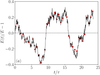
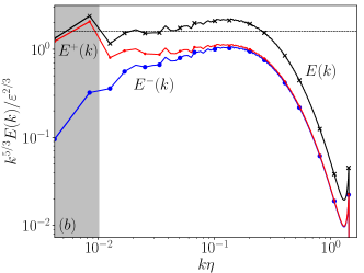
Figure 1: (a) Time evolution of the total energy normalised by its mean value, $E$. Time is given in units of large-eddy turnover time $\tau$. The red dots correspond to the sampled velocity-field configurations. (b) Time-averaged energy spectra in Kolmogorov-compensated form. The grey-shaded area indicates the forcing range. The dashed line indicates a Kolmogorov constant $C_{K}\approx 1.6$.

4 Numerical results for mean subfluxes and fluctuations

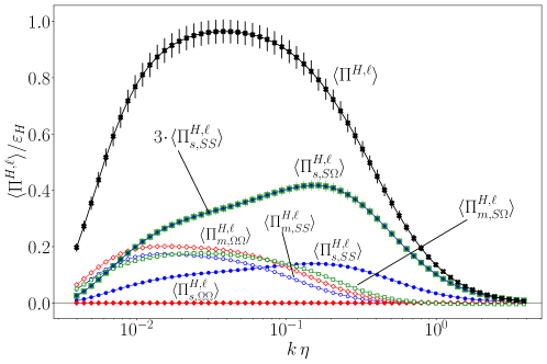
Figure 2: Decomposed helicity fluxes normalised with the mean helicity dissipation rate $\varepsilon_{H}$. Filled markers corresponds to single-scale contributions while empty symbols are related to multi-scale contributions. The error bars indicate one standard error. The subflux $\langle\Pi_{s,S\Omega}^{H,\ell}\rangle$ has been superposed with $3\langle\Pi_{s,SS}^{H,\ell}\rangle$ in order to highlight the Betchov-type relation (19).

Figure 2 shows the total helicity flux and all subfluxes, normalised by the total helicity dissipation rate $\varepsilon_{H}$. As can be seen in the figure, the term $\langle\Pi^{H,\ell}_{s,\Omega\Omega}\rangle$ is identically zero, which must be the case according to (18). Moreover, the helicity Betchov relation (19) derived here is satisfied as it must be – the terms $\langle\Pi^{H,\ell}_{s,S\Omega}\rangle$ and $3\,\langle\Pi^{H,\ell}_{s,SS}\rangle$ are visually indistinguishable, with a relative error between them of order $10^{-6}$ (not shown). A few further observations can be made from the data. The non-vanishing multi-scale terms, $\langle\Pi^{H}_{m,S\Omega}\rangle$, $\langle\Pi^{H}_{m,SS}\rangle$ and $\langle\Pi^{H}_{m,\Omega\Omega}\rangle$ are comparable in magnitude across all scales. They are approximately scale-independent in the interval $10^{-2}\leqslant k\eta\leq 10^{-1}$, with each accounting for about $15-20\%$ of the total helicity flux in this range of scales. Even though clear plateaux are not present for the two non-vanishing single-scale terms, $\langle\Pi^{H}_{s,S\Omega}\rangle$ and $\langle\Pi^{H}_{s,SS}\rangle$, one could tentatively extrapolate that at higher Re, about $30\%$ of the mean flux originates from scale-local vortex twisting and $10\%$ from vortex flattening. That is, the multi-scale contributions amount to 50%-60% and the scale-local contributions to 40-50% of the total helicity flux across scales, at least for this particular simulation.

Having discussed the mean subfluxes, we now consider the fluctuations of each subflux term, in order to quantify the level of fluctuations in each term and the presence and magnitude of helicity backscatter. Figure 3 presents standardised probability density functions (PDFs) of all helicity subfluxes at $k=\pi/\ell=20$, which is in the inertial range. These PDFs are fairly symmetric, much more so than for the kinetic energy fluxes, have wide tails, and are strongly non-Gaussian. Single- and multi-scale terms all have strong fluctuations of about 75 standard deviations. Interestingly, the subflux term $\Pi_{s,\Omega\Omega}^{H,\ell}$, which necessarily vanishes in mean (see (18)), has the strongest fluctuations (i.e., is the most intermittent). PDFs for all the other subfluxes are comparable. The symmetry is more pronounced in the single-scale rather than the multi-scale terms, as can be seen by comparison of the left and right panels of fig. 3. As all averaged fluxes (except $\langle\Pi_{s,\Omega\Omega}^{H,\ell}\rangle$ which is zero) transfer positive helicity from large to small scales, symmetry in the PDFs indicates strong backscatter of positive helicity, or forward scatter of negative helicity. The PDFs become even broader with decreasing filter scale (not shown). A comparison between the PDFs of $\Pi^{H,\ell}$ and the alternate description based on SGS stresses related to vortex stretching, $\tilde{\Pi}^{H,\ell}$, has been carried out by Yan et al. (2020), indicating more intense backscatter in the latter compared to the former. Adding or removing a total gradient can strongly reduce the negative tail of the SGS energy transfer (Vela-Martín, 2022), and the same may apply to the helicity flux.

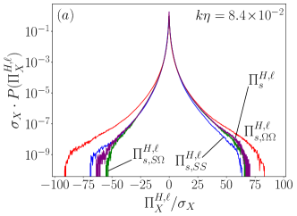
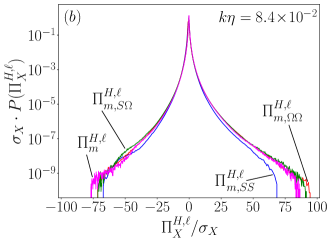
Figure 3: Standardised PDFs of helicity subfluxes $\Pi_{X}^{H,\ell}$, where $X$ refers to the subflux identifier, for (a) single-scale and (b) multi-scale contributions; $\sigma_{X}$ denotes the standard deviation of each respective term.

5 Conclusions

We have derived an exact decomposition of the helicity flux across scales in terms of interactions between vorticity gradients and velocity gradients, and in terms of their scale locality. Decomposing all gradient tensors into symmetric and anti-symmetric parts allows for a discussion and quantification of different physical mechanisms that constitute the helicity cascade. Simulation results indicate that all subfluxes transfer helicity from large to small scales, albeit with strong backscatter. In the inertial range, about 50$\%$ of the total mean helicity flux is due to the action of two scale-local processes: (i) vortex flattening and (ii) vortex twisting. We have also shown that these two effects are related in mean through a newly derived exact (Betchov-type) relation, which implies that the contribution of the former is exactly three times larger than that of the latter. Multi-scale effects account for the remaining 50$\%$, with approximate equipartition between multi-scale versions of the two aforementioned effects and multi-scale vortex entangling. Thus, it seems likely that, in LES contexts, accurate modeling of the helicity cascade should not neglect the multi-scale contributions. Although our numerical quantification of the fluxes is obtained using data from a single simulation with an inertial range of limited length, we conjecture that the results obtained are robust in the sense that we expect them to hold for flows with larger Reynolds numbers. Similar flux decompositions can be derived for magnetohydrodynamics. We will report results of these investigations elsewhere in due course.

Computational resources were provided through Scottish Academic Access on Cirrus (www.cirrus.ac.uk), and the UK Turbulence Consortium on ARCHER2 (www.archer2.ac.uk). This work received funding from the European Research Council (ERC) under the European Union’s Horizon 2020 research and innovation programme (grant agreement No 882340) and from the Priority Programme SPP 1881 “Turbulent Superstructures” of the Deutsche Forschungsgemeinschaft (DFG, Li3694/1).

Competing interests: the authors declare none.

References

- Alexakis (2017) Alexakis, A. 2017 Helically Decomposed Turbulence. J. Fluid Mech. 812, 752–770.
- Alexakis & Biferale (2018) Alexakis, A. & Biferale, L. 2018 Cascades and transitions in turbulent flows. Physics Reports 767-769, 1–101.
- Baerenzung et al. (2008) Baerenzung, J., Politano, H., Ponty, Y. & Pouquet, A. 2008 Spectral modeling of turbulent flows and the role of helicity. Phys. Rev. E. 77, 046303.
- Betchov (1956) Betchov, R. 1956 An inequality concerning the production of vorticity in isotropic turbulence. J. Fluid Mech. 1, 497.
- Biferale et al. (2012) Biferale, L., Musacchio, S. & Toschi, F. 2012 Inverse energy cascade in three-dimensional isotropic turbulence. Phys. Rev. Lett. 108, 164501.
- Biferale et al. (2013) Biferale, L., Musacchio, S. & Toschi, F. 2013 Split Energy-Helicity cascades in three dimensional Homogeneous and Isotropic Turbulence. J. Fluid Mech. 730, 309–327.
- Brandenburg (2001) Brandenburg, A. 2001 The inverse cascade and nonlinear alpha-effect in simulations of isotropic helical magnetohydrodynamic turbulence. Astrophys. J. 550, 824–840.
- Brandenburg & Subramanian (2005) Brandenburg, A. & Subramanian, K. 2005 Astrophysical magnetic fields and nonlinear dynamo theory. Phys. Reports 417, 1–209.
- Brissaud et al. (1973) Brissaud, A., Frisch, U., Léorat, J., Lesieur, M. & Mazure, A. 1973 Helicity cascades in fully developed isotropic turbulence. Phys. Fluids 16, 1366–1367.
- Carbone & Wilczek (2022) Carbone, M. & Wilczek, M. 2022 Only two Betchov homogeneity constraints exist for isotropic turbulence. J. Fluid Mech. 948, R2.
- Chen et al. (2003a) Chen, Q., Chen, S. & Eyink, G. L. 2003a The joint cascade of energy and helicity in three-dimensional turbulence. Phys. Fluids 15, 361–374.
- Chen et al. (2003b) Chen, Q., Chen, S., Eyink, G. L. & Holm, D. D. 2003b Intermittency in the joint cascade of energy and helicity. Phys. Rev. Lett. 90, 214503.
- Constantin & Majda (1988) Constantin, P. & Majda, A. 1988 The Beltrami spectrum for incompressible flows. Commun. Math. Phys. 115, 435–456.
- Deusebio & Lindborg (2014) Deusebio, E. & Lindborg, E. 2014 Helicity in the Ekman boundary layer. J. Fluid Mech. 755, 654–671.
- Eyink (2005) Eyink, G. L. 2005 Locality of turbulent cascades. Physica D 207, 91–116.
- Eyink (2006) Eyink, G. L. 2006 Multi-scale gradient expansion of the turbulent stress tensor. J. Fluid Mech. 549, 159–190.
- Germano (1992) Germano, M. 1992 Turbulence — the filtering approach. J. Fluid Mech. 238, 325–336.
- Gledzer & Chkhetiani (2015) Gledzer, E. B. & Chkhetiani, O. G. 2015 Inverse energy cascade in developed turbulence at the breaking of the symmetry of helical modes. JETP Letters 102, 465–472.
- Herring (1974) Herring, J. R. 1974 Approach of axisymmetric turbulence to isotropy. Phys. Fluids 17, 859.
- Inagaki et al. (2017) Inagaki, K., Yokoi, N. & Hamba, F. 2017 Mechanism of mean flow generation in rotating turbulence through inhomogeneous helicity. Phys. Rev. Fluids 2, 114605.
- Johnson (2020) Johnson, P. L. 2020 Energy transfer from large to small scales in turbulence by multiscale nonlinear strain and vorticity interactions. Phys. Rev. Lett. 124, 104501.
- Johnson (2021) Johnson, P. L. 2021 On the role of vorticity stretching and strain self-amplification in the turbulence energy cascade. J. Fluid Mech. 922, A3.
- Kessar et al. (2015) Kessar, M., Plunian, F., Stepanov, R. & Balarac, G. 2015 Non-Kolmogorov cascade of helicity-driven turbulence. Phys. Rev. E 92, 031004(R).
- Kraichnan (1973) Kraichnan, R. 1973 Helical turbulence and absolute equilibrium. J. Fluid Mech. 59, 745–752.
- Li et al. (2006) Li, Y., Meneveau, C., Chen, S. & Eyink, G. L. 2006 Subgrid-scale modeling of helicity and energy dissipation in helical turbulence. Phys. Rev. E. 74, 026310.
- Lilly (1986) Lilly, D. K. 1986 The structure, energetics, and propagation of rotating convective storms. Part II: Helicity and storm stabilization. J. Atmos. Sci. 43, 126.
- Linkmann (2018) Linkmann, M. 2018 Effects of helicity on dissipation in homogeneous box turbulence. J. Fluid Mech. 856, 79–102.
- Linkmann et al. (2016) Linkmann, M. F., Berera, A., McKay, M. E. & Jäger, J. 2016 Helical mode interactions and spectral energy transfer in magnetohydrodynamic turbulence. J. Fluid Mech. 791, 61–96.
- Linkmann et al. (2017) Linkmann, M. F., Sahoo, G., McKay, M. E., Berera, A. & Biferale, L. 2017 Effects of Magnetic and Kinetic Helicities on the Growth of Magnetic Fields in Laminar and Turbulent Flows by Helical Fourier Decomposition. Astrophys. J. 836, 26.
- Milanese et al. (2021) Milanese, L. M., Loureiro, N. F. & Boldyrev, S. 2021 Dynamic Phase Alignment in Navier-Stokes Turbulence. Phys. Rev. Lett. 127, 274501.
- Mininni & Pouquet (2010a) Mininni, P. D. & Pouquet, A. G. 2010a Rotating helical turbulence. I. Global evolution and spectral behavior. Phys. Fluids 22, 035105.
- Mininni & Pouquet (2010b) Mininni, P. D. & Pouquet, A. G. 2010b Rotating helical turbulence. II. Intermittency, scale invariance, and structures. Phys. Fluids 22, 035106.
- Moffatt (1969) Moffatt, H. K. 1969 The degree of knottedness of tangled vortex lines. J. Fluid Mech. 35, 117–129.
- Moffatt (2014) Moffatt, H. K. 2014 Helicity and singular structures in fluid dynamics. Proc. Natl. Acad. Sci. 111 (10), 3663–3670.
- Sahoo et al. (2017) Sahoo, G., Alexakis, A. & Biferale, L. 2017 Discontinuous transition from direct to inverse cascade in three-dimensional turbulence. Phys. Rev. Lett. 118, 164501.
- Sahoo et al. (2015) Sahoo, G., Bonaccorso, F. & Biferale, L. 2015 Role of helicity for large- and small-scale turbulent fluctuations. Phys. Rev. E 92, 051002.
- Scheeler et al. (2017) Scheeler, M. W., van Rees, W. M., Kedia, H., Kleckner, D. & Irvine, W. T. M. 2017 Complete measurement of helicity and its dynamics in vortix tubes. Science 357, 487–491.
- Steenbeck et al. (1966) Steenbeck, M., Krause, F. & Rädler, K.-H. 1966 Berechnung der mittleren Lorentz-Feldstärke v x B für ein elektrisch leitendes Medium in turbulenter, durch Coriolis-Kräfte beeinflußter Bewegung. Z. Naturforsch. A 21, 369.
- Stepanov et al. (2015) Stepanov, R., Golbraikh, E., Frick, P. & Shestakov, A. 2015 Hindered energy cascade in highly helical isotropic turbulence. Phys. Rev. Lett. 115, 234501.
- Tobias et al. (2013) Tobias, S. M., Cattaneo, F. & Boldyrev, S. 2013 MHD Dynamos and Turbulence. In Ten Chapters in Turbulence. Cambridge University Press.
- Vela-Martín (2022) Vela-Martín, A. 2022 Subgrid-scale models of isotropic turbulence need not produce energy backscatter. J. Fluid Mech. 937, A14.
- Waleffe (1992) Waleffe, F. 1992 The nature of triad interactions in homogeneous turbulence. Phys. Fluids A 4, 350–363.
- Yan et al. (2020) Yan, Z., Li, X., Yu, C., Wang, J. & Chen, S. 2020 Dual channels of helicity cascade in turbulent flows. J. Fluid Mech. 894, R2.
- Yokoi & Yoshizawa (1993) Yokoi, N. & Yoshizawa, A. 1993 Statistical analysis of the effects of helicity in inhomogeneous turbulence. Phys. Fluids A 5, 464.
- Yu et al. (2022) Yu, C, Hu, R., Yan, Z. & Li, X. 2022 Helicity distributions and transfer in turbulent channel flows with streamwise rotation. J. Fluid Mech. 940, A18.