A thin film model for meniscus evolution

Abstract

In this paper, we discuss a particular model arising from sinking of a rigid solid into a thin film of fluid, i.e. a fluid contained between two solid surfaces and part of the fluid surface is in contact with the air. The fluid is governed by Navier-Stokes equation, while the contact point, i.e. where the gas, liquid and solid meet, is assumed to be given by a constant, non-zero contact angle. We consider a scaling limit of the fluid thickness (lubrication approximation) and the contact angle between the fluid-solid and the fluid-gas interfaces is close to $\pi$. This resulting model is a free boundary problem for the equation $h_{t}+(h^{3}h_{xxx})_{x}=0$, for which we have $h>0$ at the contact point (different from the usual thin film equation with $h=0$ at the contact point). We show that this fourth order quasilinear (non-degenerate) parabolic equation, together with the so-called partial wetting condition at the contact point, is well-posed. Also the contact point in our thin film equation can actually move, contrary to the classical thin film equation for a droplet arising from no-slip condition. Furthermore, we show the global stability of steady state solutions in a periodic setting.

1 Introduction

In this paper, we investigate a particular thin film model, where a rigid solid enters a liquid film (cf. Figure 1), leading to movement of the contact point and the formation of a meniscus, as the initial state is out of equilibrium. This free boundary problem gives rise to the following fourth order non-linear parabolic equation, in one dimension,

$$\partial_{t}h+\partial_{x}(h^{3}\partial^{3}_{x}h)=0\qquad\text{ in }x>\Lambda,t>0,$$ (1.1a)

along with the boundary conditions,

$$h=g,\qquad\partial_{x}h=\partial_{x}g-k,\qquad h\partial_{x}^{3}h=-\frac{6\Lambda\;\partial_{t}g}{g^{2}}\quad\qquad\text{ at }x=\Lambda,t>0.$$ (1.1b)

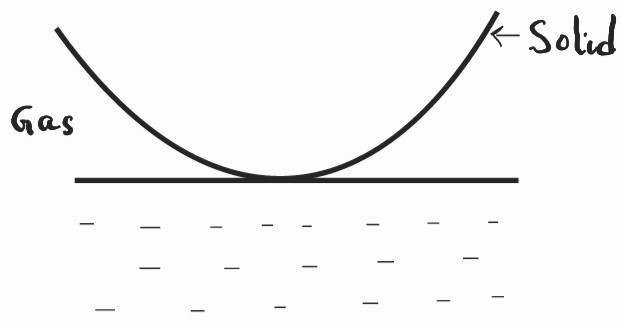
Figure 1: General meniscus formation

Here $h=h(x,t)$ is the height of the fluid film, $\Lambda=\Lambda(t)$ is the contact point (which is a free boundary in one dimension), $k$ is the fixed contact angle (rescaled), i.e. the angle between the fluid-solid and the fluid-air interfaces, and $g=g(x,t)$ is the profile of the rigid solid. Deduction of the above system is elaborated in Section 2. Here the situation in one spatial dimension is studied only, although one may consider general dimension as well (physically relevant cases correspond to $d=1$ or $2$). The study of fluid problems involving free boundary evolution mostly concerns with an interface between two phases (cf. [19]), whereas the interest of the current paper is the situation where three phases of matter meet (typically, fluid-solid-air), generating a contact line/point. The main differences between the model considered here with other classical triple junction model is pointed out later.

Equation (1.1a):

Let us first discuss the equation (1.1a) which can be viewed as a particular case of the general class of thin film equations

$$\partial_{t}h+\partial_{x}(f(h)\partial_{x}^{3}h)=0\quad\text{ in }\{h>0\}.$$ (1.2)

Equations of the form (1.2) are typically obtained by lubrication approximation of the motion of a two-dimensional viscous fluid droplet, spreading over a solid substrate by the effect of surface tension (cf. [2]). Classical macroscopic fluid mechanics to model such phenomena imposes the no-slip boundary condition at the fluid-solid interface, that is the velocity of the fluid must be equal to that of the solid substrate in contact with. This corresponds to the case $f(h)=h^{3}$. However, this condition can not hold at the moving contact point/triple junction where the solid, liquid and gas, three phases meet. It is known to give rise to a non-integrable singularity at the contact point (cf. [11]) which further implies that boundary of the film (i.e. the triple junction) can not move in time (no slip paradox). On other hand, Navier slip condition (corresponds to the case $f(h)=h^{2}$), proposed by Navier [14], which allows the fluid to slip over the solid surface (characterized by a slip parameter), resolves such paradoxical phenomena (cf. [15] for a discussion in this direction).

Note that equation (1.2) can also be viewed as a higher order version of the Porous medium equation

$$\partial_{t}h-\partial_{x}(h^{n}\partial_{x}h)=0,\quad n>0.$$

However, the standard techniques used for such second order degenerate parabolic equations (such as Maximum principle) are not available for the higher order counterpart which makes the analysis more difficult for the later (cf. [7]).

Equation (1.1b):

Next let us discuss the boundary conditions in (1.1b). The first condition gives the position of the free boundary, whereas the second one determines the slope at the free boundary (contact angle condition). The case where the (equilibrium) contact angle is given by a non-zero constant, determined by Young’s law (balance between interfacial energies) (cf. [3]), is known as partial wetting, whereas the zero contact angle is referred as complete wetting. This work takes into account both the possibilities. There are also notions of dynamic/apparent contact angle (cf. [10, 16]). The third boundary condition comes from a matching condition with the internal region (i.e. the fluid region bounded between solid parts), while in the standard setting of a droplet, a third condition is deduced from matching the velocity of the contact point. This would lead to an over-determined problem for a fourth order operator with fixed boundary, but not for the free boundary problem where the boundary is an unknown a priori.

State of the art. All the literature available in the context of thin film equation for contact angle problem consider either compactly supported initial data (droplet case) or an unbounded support with single free boundary. Thus the standard condition $h=0$ of the vanishing fluid height at the free boundary makes the equation $\partial_{t}h+\partial_{x}(h^{n}\partial^{3}_{x}h)=0$ singular/degenerate. Following the pioneering work of Bernis and Friedman [1], several results has been established for (1.2), considering different forms of $f$, for example in [7], [6]-[8], [12]-[13], [17]. The above references are not claimed to be exhaustive. We also point out the work [9] where stability of a global solution for the general contact line problem for Stokes equation has been discussed.

The current work is concerned with a different thin film model, deduced from the no-slip boundary condition assumption at the fluid-solid interface. The film height being $h>0$ at the contact point makes our model non-degenerate, unlike the standard thin film equation as discussed above. The result shows well-posedness as well as the possibility of moving contact point. Moreover, no paradox arises in spite that the contact point moves. The reason of such behavior in this case is that the contact angle is very close to $\pi$. As pointed out by Solonnikov in [20], the paradox gets resolved in the case of contact angle $\pi$. The main contribution of the paper is to bring forward this particular interesting yet simple situation involving the evolution of triple junction and the discussion of different behavior in contrast to the known cases. This observation intrigued our curiosity to analyze the model in detail.

Structure of the paper. We first deduce a general thin film model describing the above particular situation of meniscus formation under the classical approach in Section 2. The arguments used in this derivation are standard. Still we write this derivation in detail, since we did not find any suitable reference for such model. In Section 3, the local well-posedness result is established, for the particular case of no-slip boundary condition. The system being non-degenerate, standard theory for fourth order parabolic quasilinear equation can be employed. Nevertheless, obtaining suitable regularity (in time) in order to closing the final fixed point argument is not straight-forward (cf. Remark 3.1). Finally we obtain the asymptotic behavior of a solution, in periodic setting, in Section 4. By looking at perturbations of a steady state of (1.1a)-(1.1b), existence of a unique global solution is obtained with the help of a priori energy estimates. As long as the initial data remains close (in certain norm) to the stationary solution, the local solution of the thin film model converges to the steady state for all time.

1.1 Main results

Our first result concerns existence of a local in time solution to the following thin film equation with moving contact point and prescribed contact angle (including complete wetting case)

$$\partial_{t}h+\partial_{x}(h^{3}\partial^{3}_{x}h)=0 \text{ in }x>\Lambda,t>0,$$ (1.3)

$$h=g,\quad\partial_{x}h=\partial_{x}g-k,\quad h\;\partial_{x}^{3}h=-6\Lambda\frac{\partial_{t}g}{g^{2}} \text{ at }x=\Lambda,t>0,$$

$$h\to 1 \text{ as }\ x\to\infty,t>0,$$

$$h=h_{0} \text{ at }\ t=0,x>\Lambda_{0}.$$

Here $\Lambda_{0}=\Lambda(0)$ denotes the initial position of the contact point.

Theorem 1.1

For any initial data $(h_{0},\Lambda_{0})$, satisfying compatibility conditions, there exists a unique strong solution $(h,\Lambda)$, for short time, of the free boundary problem (1.3).

Rigorous statement and proof of the above theorem is given in Section 3. Next we consider the system (1.3) over an interval $(0,2L)$ (in order to have a bounded domain), symmetric with respect to $x=L$ and with periodic boundary conditions. Precisely,

$$\partial_{t}h+\partial_{x}(h^{3}\partial^{3}_{x}h)=0 \text{ in }\ x\in(\Lambda,L),t>0,$$ (1.4)

$$h=g,\quad\partial_{x}h=\partial_{x}g-k,\quad h\;\partial_{x}^{3}h=0 \text{ at }\ x=\Lambda,t>0,$$

$$\partial_{x}h=0 \text{ at }\ x=L,t>0,$$

$$h=h_{0} \text{ at }\ t=0,x\in(\Lambda_{0},L),$$

$$h(x,t)=h(x+2L,t),\quad g(x,t)=g(x+2L,t), \qquad x,t>0.$$

The free interface $h(x,t)$ is defined over the domain $(\Lambda,2L-\Lambda)$ in this case. Also we assume here that the solid is not moving, i.e. $\partial_{t}g=0$. Such a solution preserves mass for all time $t>0$ (cf. Section 4.1). Then, for a given volume $V_{0}$, a steady state $(\overline{h},\overline{\Lambda})$ of (1.4) is characterized by

$$\partial_{x}(\overline{h}^{3}\partial^{3}_{x}\overline{h})=0\ \text{ in }\ x\in(\overline{\Lambda},L),$$

subject to the boundary conditions

$$\overline{h}=g,\ \partial_{x}\overline{h}=\partial_{x}g-k,\ \partial_{x}^{3}\overline{h}=0\quad\text{ at }x=\overline{\Lambda}\quad\text{ and }\quad\partial_{x}\overline{h}=0\quad\text{ at }x=L.$$

We refer to (4.8) for an explicit description of the steady state. Stability of this steady state for small perturbation is obtained as below, we refer to Section 4.3 for rigorous statement and proof.

Theorem 1.2

For initial data close enough to the steady state of (1.4), there is a unique global solution $(h,\Lambda)$ of the problem (1.4) which converges to the steady state as $t\to\infty$.

2 Lubrication approximation

In this section, we elaborate the thin film approximation of the original three phase free boundary problem in consideration.

Original model: Let us consider a horizontal, two-dimensional thin film of viscous, incompressible Newtonian fluid, of thickness $H$ at the initial time and a rigid solid (locally convex) touching the film (cf. Figure 2). As the solid enters the liquid, the contact point moves and makes an angle $(\pi-\theta)$, $\theta>0$, between the liquid-solid and the liquid-gas interface. The liquid-gas interface is described by $y=h(x,t)$ and the liquid-solid boundary is given by $y=g(x,t)$. One may think of particular cases, for example $g=H\left(1-\left(\frac{t}{t_{0}}\right)^{n}\right)$ with $n>0$ where $t_{0}$ is the time scale that characterises the motion of the solid moving down. Here $n=1$ corresponds to the solid moving with constant velocity, while $n=2$ corresponds to the case of constant acceleration. A particular case of wedge-shaped solid (in the form $g(x,t)=\tilde{h}(t)+c|x|$) has been mentioned in [18, Fig 6] in a context of correct modelling approach describing the creation of contact angle. The free interface makes an angle $\tilde{\theta}$ with the horizontal plane (cf. Figure 2). Therefore, $\tan\tilde{\theta}=-\partial_{x}h$ and $\theta=-\arctan(\partial_{x}h)+\arctan(\partial_{x}g)$. To obtain the lubrication approximation, we need to assume that the two angles $\theta$ and $\tilde{\theta}$ are very small and of the same order, which means that the contact angle $(\pi-\theta)$ is close to $\pi$ in this setting. Note that the thin film approximation would not be valid if $\tilde{\theta}$ is large. The contact points are given by $s_{i}=(\Lambda_{i}(t),y)$. Finally, we assume the far field condition $h\to H$ as $|x|\to\infty$.

Let $\mathbf{v}^{L}=(u,v)$ be the velocity of the fluid, with constant density $\varrho^{L}$, viscosity $\mu^{L}$ and pressure $p^{L}$, governed by the Navier-Stokes equations, while the solid motion is governed by the translational velocity only $\mathbf{v}^{S}(t)$, vertically downward. Let us consider the bottom part of the fluid domain as a reference configuration, i.e. at $y=0$.

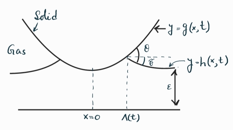
Figure 2: Thin Film approximation with contact points

As we assume a symmetric configuration with respect to $y$-axis (for simplicity), it is enough to analyse the situation for $x>0$ only. Therefore, in the following, we call the contact point $\Lambda$ instead of $\Lambda_{1}$.

Further assumptions:

Let the solid $g$ be smooth in a neighborhood of the initial contact point $\Lambda_{0}$. Moreover, $g>0$ for all $x,t\geq 0$, i.e. the solid never touches the bottom of the fluid domain which may lead to further singularities.

In the framework of classical fluid mechanics, conditions at contact lines are considered only at equilibrium, i.e. in the situations where the contact line is not moving with respect to the bulk phases. Also we consider here the Navier slip condition at the fluid-solid interface, for a general framework, which covers both the no-slip and the full-slip condition. We formulate these conditions below (cf. [4, Section 2.4]).

in the liquid:

$$\mathrm{div}_{\mathbf{x}}\;\mathbf{v}^{L}=0,\qquad\varrho^{L}\left(\partial_{t}\mathbf{v}^{L}+\mathbf{v}^{L}\cdot\nabla_{\mathbf{x}}\mathbf{v}^{L}\right)=\mu^{L}\Delta\mathbf{v}^{L}-\nabla_{\mathbf{x}}p^{L};$$ (2.1)

at the liquid-gas interface: $y=h(x,t),x>\Lambda(t)$:

$$V_{n}=\mathbf{v}^{L}\cdot\mathbf{n}_{1},\qquad\left(p^{G}-p^{L}\right)+2\mu^{L}\left[\mathbb{D}\mathbf{v}^{L}\cdot\mathbf{n}_{1}\right]\cdot\mathbf{n}_{1}+p^{s}\kappa=0,\qquad\left[\mathbb{D}\mathbf{v}^{L}\cdot\mathbf{n}_{1}\right]_{\tau}=0;$$ (2.2)

at the liquid-solid interface $\{y=0\}\cup\{y=g(x,t),0<x<\Lambda(t)\}$:

$$\left(\mathbf{v}^{L}-\mathbf{v}^{S}\right)\cdot\mathbf{n}_{2}=0,\qquad 2\mu^{L}\left[\mathbb{D}\mathbf{v}^{L}\cdot\mathbf{n}_{2}\right]_{\tau}=\beta\left(\mathbf{v}^{L}_{\tau}-\mathbf{v}^{S}_{\tau}\right);$$ (2.3)

at the triple junction $x=\Lambda(t)$:

$$h=g,\qquad\arctan(\partial_{x}h)=\arctan(\partial_{x}g)-\theta.$$ (2.4)

Here $p^{s}$ is the (constant) surface tension, $\kappa$ is the curvature of the free interface, $p^{G}$ is the constant pressure of the gas and $\mathbf{n}_{i},i=1,2$ are the unit normal vectors, inward with respect to the fluid domain. We do not distinguish here between the slip-coefficients appearing at the lower and upper fluid-solid interface and denote both of them by $\beta$ only. In principle, they might be different. We further assume for simplicity that the lower boundary $y=0$ is fixed, i.e. $\mathbf{v}^{S}=0$ at $y=0$.

Also, we must have the matching condition for the initial data,

$$h(x,0)=H\qquad\text{ at }t=0.$$ (2.5)

Further, due to the symmetry assumption of the considered configuration, one has,

$$u=0\qquad\text{ on }x=0.$$ (2.6)

Now let us introduce the length scale as $L=\frac{H}{\varepsilon}$ where $\varepsilon>0$ is small. Then the usual scaling of the variables are given by,

$$(\overline{x},\overline{y})=\left(\frac{x}{L},\frac{y}{H}\right) \overline{\Lambda}=\frac{1}{L}\Lambda, \overline{h}=\frac{h}{H},\overline{g}=\frac{g}{H}$$

$$\overline{t}=\frac{\sigma}{L\mu}t, (\overline{u},\overline{v})=\left(\frac{\mu}{\sigma}u,\frac{\mu}{\varepsilon\sigma}v\right), \overline{p}=\frac{\varepsilon^{2}L}{\sigma}p,\theta=k\varepsilon,$$

with $\sigma=-\varepsilon^{3}p^{s}$ is the scaled surface tension.

Rescaled system: Under these scaling, we obtain the following approximated system of equations from (2.1)-(2.4),

$$\partial_{\overline{x}}\overline{u}+\partial_{\overline{y}}\overline{v}=0,\qquad\partial^{2}_{\overline{y}}\overline{u}=\partial_{\overline{x}}\overline{p},\qquad\partial_{\overline{y}}\overline{p}=0,$$ (2.7a)

$$\hskip 153.07596pt\text{in }(\overline{x},\overline{y})\in(0,\overline{\Lambda})\times(0,\overline{g})\cup(\overline{\Lambda},\infty)\times(0,\overline{h}),$$

$$\partial_{\overline{t}}\overline{h}+\overline{u}\;\partial_{\overline{x}}\overline{h}-\overline{v}=0,\qquad\overline{p}=-\partial^{2}_{\overline{x}}\overline{h},\qquad\partial_{\overline{y}}\overline{u}=0,\hskip 11.38092pt\qquad\text{ on }\overline{x}>\overline{\Lambda},\;\overline{y}=\overline{h},$$ (2.7b)

$$\overline{v}=0,\qquad\partial_{\overline{y}}\overline{u}=\beta\;\overline{u},\hskip 179.25244pt\qquad\text{ on }\overline{y}=0,$$ (2.7c)

$$\partial_{\overline{x}}\overline{g}\;\overline{u}=\overline{v}-\partial_{\overline{t}}\overline{g},\qquad\partial_{\overline{y}}\overline{u}+\overline{\beta}\;\overline{u}=0,\hskip 79.6678pt\qquad\text{on }\overline{x}<\overline{\Lambda},\;\overline{y}=\overline{g},$$ (2.7d)

$$\overline{h}=\overline{g},\qquad\partial_{\overline{x}}\overline{h}=\partial_{\overline{x}}\overline{g}-k,\hskip 159.0508pt\qquad\text{ at }\overline{x}=\overline{\Lambda},$$ (2.7e)

$$\overline{h}\to 1\hskip 256.0748pt\qquad\text{as }\overline{x}\to\infty,$$ (2.7f)

where the rescaled slip coefficient $\overline{\beta}=\frac{\varepsilon\beta L}{\mu}=O(1)$. The system is complemented by equations (2.5), (2.6).

Indeed, the incompressibility condition $(\ref{1})_{1}$ remains same in the new variables, leading to $(\ref{19})_{1}$. The Navier-Stokes equation $(\ref{1})_{2}$ in the first component becomes,

$$\underset{\mathrm{Re}}{\underbrace{\varrho^{L}\frac{\sigma}{\mu^{L}}\frac{L}{\mu^{L}}}}\left(\partial_{\overline{t}}\overline{u}+\overline{u}\partial_{\overline{x}}\overline{u}+\overline{v}\partial_{\overline{y}}\overline{u}\right)=\Big{(}\partial_{\overline{x}}^{2}\overline{u}+\frac{1}{\varepsilon^{2}}\partial_{\overline{y}}^{2}\overline{u}\Big{)}-\frac{1}{\varepsilon^{2}}\partial_{\overline{x}}\overline{p}.$$

Thus in the limit $\varepsilon\to 0$, both the time derivative and the non-linear term vanish compared to the viscous term when Reynolds number satisfies $\varepsilon^{2}\mathrm{Re}\ll 1$ and one obtains $(\ref{19})_{2}$. Similarly the second component of Navier-Stokes equation reduces to $(\ref{19})_{3}$.

Next we discuss the boundary conditions. At the liquid-gas interface $\overline{y}=\overline{h}(\overline{x},\overline{t}),\overline{x}>\overline{\Lambda}(\overline{t})$, the unit normal and tangent vectors and the curvature have the following expressions,

$$\mathbf{n}_{1}=\frac{\left(\varepsilon\partial_{\overline{x}}\overline{h},-1\right)}{\sqrt{(1+\varepsilon^{2}|\partial_{\overline{x}}\overline{h}|^{2})}},\quad\mathbf{\tau}=\frac{\left(1,\varepsilon\partial_{\overline{x}}\overline{h}\right)}{\sqrt{(1+\varepsilon^{2}|\partial_{\overline{x}}\overline{h}|^{2})}}\quad\text{ and }\quad\kappa=\frac{\varepsilon\partial^{2}_{\overline{x}}\overline{h}}{L\left(1+\varepsilon^{2}|\partial_{\overline{x}}\overline{h}|^{2}\right)^{3/2}}.$$ (2.8)

The kinematic boundary condition $(\ref{6})_{1}$ reduces to the non-dimensional form $(\ref{41})_{1}$. Also the rate of strain tensor becomes, in the new variables,

$$\mathbb{D}\mathbf{v}^{L}=\frac{1}{2}\begin{bmatrix}2\partial_{x}u&\partial_{y}u+\partial_{x}v\\ \partial_{y}u+\partial_{x}v&2\partial_{y}v\end{bmatrix}=\frac{1}{2}\frac{\sigma}{L\mu}\begin{bmatrix}2\partial_{\overline{x}}\overline{u}&\frac{1}{\varepsilon}\partial_{\overline{y}}\overline{u}+\varepsilon\partial_{\overline{x}}\overline{v}\\ \frac{1}{\varepsilon}\partial_{\overline{y}}\overline{u}+\varepsilon\partial_{\overline{x}}\overline{v}&2\partial_{\overline{y}}\overline{v}\end{bmatrix}.$$

Therefore, the normal and the tangential stress on the surface $\overline{y}=\overline{h}(\overline{x},\overline{t})$ are given by,

$$\left[\mathbb{D}\mathbf{v}^{L}\cdot\mathbf{n}_{1}\right]\cdot\mathbf{n}_{1}=\frac{\sigma}{L\mu}\frac{1}{\left(1+\varepsilon^{2}|\partial_{\overline{x}}\overline{h}|^{2}\right)}\left(-\partial_{\overline{y}}\overline{u}\;\partial_{\overline{x}}\overline{h}+\partial_{\overline{y}}\overline{v}+O(\varepsilon^{2})\right),$$ (2.9)

and

$$\left[\mathbb{D}\mathbf{v}^{L}\cdot\mathbf{n}_{1}\right]\cdot\mathbf{\tau}=\frac{\sigma}{L\mu}\frac{1}{2}\frac{1}{\left(1+\varepsilon^{2}|\partial_{\overline{x}}\overline{h}|^{2}\right)}\left(-\frac{1}{\varepsilon}\partial_{\overline{y}}\overline{u}+O(\varepsilon)\right).$$ (2.10)

Then, equation $(\ref{6})_{2}$ becomes, with the help of (2.8) and (2.9),

$$p^{G}-\frac{\sigma}{\varepsilon^{2}L}\overline{p}+2\frac{\sigma}{L}\frac{1}{\left(1+\varepsilon^{2}|\partial_{\overline{x}}\overline{h}|^{2}\right)}\left(-\partial_{\overline{y}}\overline{u}\;\partial_{\overline{x}}\overline{h}+\partial_{\overline{y}}\overline{v}+O(\varepsilon^{2})\right)-\frac{\sigma}{\varepsilon^{3}}\frac{\varepsilon\;\partial^{2}_{\overline{x}}\overline{h}}{L\left(1+\varepsilon^{2}|\partial_{\overline{x}}\overline{h}|^{2}\right)^{3/2}}=0.$$

Now with the assumption that $\sigma=O(1)$, one obtains in the limit $(\ref{41})_{2}$. For equation $(\ref{6})_{3}$, one gets $(\ref{41})_{3}$ using the expression (2.10).

At the liquid-solid interface, with $\mathbf{n}_{2}=(0,1),\tau=(1,0)$ at the bottom part $y=0$, the conditions (2.3) read as,

$$v=0,\qquad\mu^{L}(\partial_{y}u+\partial_{x}v)=\beta u\qquad\text{ at }y=0,$$

which then convert into (2.7c). Similarly, at the upper fluid-solid interface, the normal and tangent vectors being,

$$\mathbf{n}_{2}=\frac{(\partial_{x}g,-1)}{\sqrt{1+|\partial_{x}g|^{2}}},\qquad\tau=\frac{(1,\partial_{x}g)}{\sqrt{1+|\partial_{x}g|^{2}}},$$

and $\mathbf{v}^{S}=(0,\partial_{t}g)$, the boundary conditions (2.3) transform into the non-dimensional form (2.7d).

The conditions at the contact point (2.4) transform into (2.7e).

Thin film equations: The thin film model can now be derived from (2.7a)-(2.7f), together with the boundary conditions and initial data as,

$$\partial_{t}h+\partial_{x}\Big{(}\Big{(}\frac{h}{3}+\frac{1}{\beta}\Big{)}h^{2}\partial^{3}_{x}h\Big{)}=0,\qquad \text{ in }x>\Lambda,$$ (2.11a)

$$h=g,\qquad\partial_{x}h=\partial_{x}g-k,\qquad \text{ at }x=\Lambda,$$ (2.11b)

$$h\to 1,\qquad \text{ as }\ x\to\infty,$$ (2.11c)

$$h=1,\qquad \text{ at }\ t=0.$$ (2.11d)

The deduction of the above system is explained in the following (omitting the bar here onwards). Integrating $(\ref{19})_{2}$ twice gives the profile of the horizontal velocity,

$$u(x,y)=\frac{1}{2}\partial_{x}p\;y^{2}+A(x,t)y+B(x,t),\qquad x>0,$$ (2.12)

where the constants $A,B$ are to be determined. The condition at the lower boundary $(\ref{bottomBC})_{2}$ implies,

$$A=\beta B,\qquad x>0.$$ (2.13)

Also the condition at the free boundary $(\ref{41})_{3}$ yields,

$$A=-\partial_{x}p\;h,\qquad\text{therefore, }\quad B=-\frac{1}{\beta}\partial_{x}p\;h,\qquad x>\Lambda.$$ (2.14)

Further, as the pressure is independent of $y$ due to $(\ref{19})_{3}$, the horizontal velocity (2.12) becomes, together with (2.14) and $(\ref{41})_{2}$,

$$u=\frac{1}{2}\partial^{3}_{x}h\left((2h-y)y+\frac{2}{\beta}h\right),\qquad x>\Lambda.$$ (2.15)

Next $(\ref{19})_{1}$ and $(\ref{bottomBC})_{1}$ give,

$$v|_{y=h}=-\int\displaylimits_{0}^{h}{\partial_{x}u\;\mathrm{d}y},\qquad x>\Lambda.$$

Thus from $(\ref{41})_{1}$, we obtain,

$$\partial_{t}h+\partial_{x}\Big{(}\int\displaylimits_{0}^{h}{u\;\mathrm{d}y}\Big{)}=0,\qquad x>\Lambda.$$

Substituting the velocity profile (2.15) into the above relation finally gives the thin film equation (2.11a). The contact line condition (2.11b) is nothing but (2.7e) and the initial data (2.11d) follows from (2.5).

Inner region: In order to determine the dynamics of the contact point fully, we need to prescribe sufficient conditions in the inner region $x<\Lambda$ as well. To do so, the condition at the fluid-solid interface $(\ref{uppersolidBC})_{2}$, together with the condition (2.13), for $x<\Lambda,y=g$, which is

$$\left[\partial_{x}p\;g+A\right]+\beta\left[\frac{1}{2}\partial_{x}p\;g^{2}+A\;g+\frac{A}{\beta}\right]=0,$$

gives a relation between $\partial_{x}p$ and $A$ for $x\in(0,\Lambda)$, that is

$$\partial_{x}p=-\frac{2A}{g}.$$ (2.16)

Also, the incompressibility condition $(\ref{19})_{1}$ gives an expression for the normal velocity for $x\in\left(0,\Lambda\right)$,

$$v\arrowvert_{y=g}=-\int\displaylimits_{0}^{\tilde{h}}{\partial_{x}u\;\mathrm{d}y}=-g\left[\frac{1}{6}\partial^{2}_{x}p\;g^{2}+\frac{1}{2}\partial_{x}A\;g+\frac{1}{\beta}\partial_{x}A\right].$$

Thus the condition $(\ref{uppersolidBC})_{1}$ implies, for $x\in(0,\Lambda)$,

$$\partial_{x}g\left[\frac{1}{2}\partial_{x}p\;g^{2}+A\left(g+\frac{1}{\beta}\right)\right]+\partial_{t}g+g\left[\frac{1}{6}\partial^{2}_{x}p\;g^{2}+\frac{1}{2}\partial_{x}A\;g+\frac{1}{\beta}\partial_{x}A\right]=0.$$

The above equation together with the relation (2.16) yields an ODE for $A$ with rational coefficients,

$$\partial_{x}A+r_{1}(x,t)\;A+r_{2}(x,t)=0,\qquad x<\Lambda,$$ (2.17)

where

$$r_{1}(x,t)=\frac{\partial_{x}g\left(\frac{1}{\beta}+\frac{1}{3}g\right)}{g\left(\frac{1}{\beta}+\frac{1}{6}g\right)},\quad r_{2}(x,t)=\frac{\partial_{t}g}{g\left(\frac{1}{\beta}+\frac{1}{6}g\right)}.$$

Also, due to the symmetry assumption (2.6), we have the boundary condition

$$A(x,t)=0\qquad\text{ at }x=0.$$

Therefore, the ODE (2.17) determines $A$ and in turn $\partial_{x}p$ in the inner region $x\in(0,\Lambda)$. Here we assume that the horizontal velocity $u$ is continuous, thus the relation (2.12) holds at $x=0$ as well. Moreover, the continuity of $u$ at $\Lambda$ further imposes the condition

$$A=h\;\partial_{x}^{3}h\qquad\text{ at }x=\Lambda.$$ (2.18)

This above relation (2.18), together with the thin film equations (2.11a)-(2.11d) determines fully the dynamics and the position of the contact point. This thin film system is described for a particular case of wedge-shaped solid, without its detailed derivation, in [5, Section 3.3].

3 Local well-posedness for no-slip condition

3.1 Notations and functional settings

Let $C_{0}[0,\infty)$ denote the Banach space of continuous, bounded functions on $[0,\infty)$ and tending to $0$ as $x\to\infty$, together with the supremum norm on $[0,\infty)$. The space $C^{k}[0,\infty),k\in\mathbb{N}$ of functions with $k$ times continuous and bounded derivatives is endowed with the standard norm

$$\|v\|_{C^{k}[0,\infty)}:=\sum_{m=0}^{k}\|\partial^{m}v\|_{C[0,\infty)}.$$

We write $C[0,\infty)\equiv C^{0}[0,\infty)$ for the space of all continuous, bounded functions on $[0,\infty)$. The Banach space of $\rho$-Hölder continuous functions $C^{\rho}[0,\infty),C^{k+\rho}[0,\infty)$ for $k\in\mathbb{N},\rho\in(0,1)$, is defined by

$$C^{\rho}[0,\infty):=\{v\in C[0,\infty):[v]_{\rho}:=\sup_{\underset{x\neq y}{x,y\in[0,\infty)}}\frac{|v(x)-v(y)|}{|x-y|^{\rho}}<\infty\},$$

together with the norm

$$\|v\|_{C^{\rho}[0,\infty)}:=\|v\|_{C[0,\infty)}+[v]_{\rho},$$

and

$$C^{k+\rho}[0,\infty):=\{v\in C^{k}[0,\infty):[\partial^{k}v]_{\rho}<\infty\},$$

with the norm

$$\|v\|_{C^{k+\rho}[0,\infty)}:=\|v\|_{C^{k}[0,\infty)}+[\partial^{k}v]_{\rho}.$$

For $\rho=1$, the above notions coincide with the class of Lipschitz functions which we denote by $C^{1-}[0,\infty)$. Sometimes we omit the underlying space $[0,\infty)$ below which should not cause any confusion.

3.2 Reduction to a fixed domain

We assume the no-slip boundary condition at the fluid-solid interface, i.e. $\frac{1}{\beta}=0$. We will show the local and global well-posedness for this reduced problem. As mentioned in the introduction, such result is in contrast with the classical thin film equation (for droplet) with no-slip condition.

Using the time scaling $t\to 3t,t_{0}\to 3t_{0}$, the thin film model (2.11a)-(2.11d) reduces to,

$$\partial_{t}h+\partial_{x}(h^{3}\partial^{3}_{x}h)=0\qquad \text{ in }x>\Lambda,t>0,$$

$$h=g,\qquad\partial_{x}h=\partial_{x}g-k,\qquad h\;\partial_{x}^{3}h=A\qquad \text{ at }x=\Lambda,t>0,$$

$$h\to 1\qquad \text{ as }\ x\to\infty,t>0,$$

$$h=1\qquad \text{ at }\ t=0,x>\Lambda_{0},$$

where $A$ solves the ODE in $(0,\Lambda)$,

$$\partial_{x}A+2\frac{\partial_{x}g}{g}A+6\frac{\partial_{t}g}{g^{2}}=0,\qquad A(0,t)=0.$$ (3.1)

Solving (3.1) gives,

$$A(x,t)=-6x\frac{\partial_{t}g}{g^{2}}.$$

Thus, we obtain the system (1.3). Recall that we have $g>0$ for all $x,t\geq 0$ by assumption.

Without loss of generality, we assume $\Lambda(0)=0$. Hence, for some $\delta>0$, there exists $T_{\delta}>0$ such that

$$|\Lambda(t)|\leq\delta^{2}\qquad\text{ and }\quad|\dot{\Lambda}(t)|\leq C\qquad\text{ for }\ t\in[0,T_{\delta}].$$ (3.2)

For such a $\delta$ fixed, let us now consider a cut-off function $\xi_{\delta}\in C_{c}^{\infty}(\mathbb{R})$ i.e.

$$\xi_{\delta}(s)=\begin{cases}1,&\quad\text{ if }\ 0\leq s\leq\delta,\\ 0,&\quad\text{ if }\ s\geq 2\delta,\end{cases}\qquad\text{ such that }\quad|\xi^{\prime}_{\delta}|\leq\frac{C}{\delta},$$

and the following bijection

$$Q_{\Lambda}(x,t)=(x-\Lambda(t))\xi_{\delta}(x-\Lambda(t))+x(1-\xi_{\delta}(x-\Lambda(t))).$$

Denoting by

$$\overline{x}=Q_{\Lambda}(x,t)\qquad\text{ and }\qquad H(\overline{x},t)=h(x,t),$$

one can compute the derivatives in the new coordinate as,

$$\partial_{t}h=\partial_{t}H+\dot{\Lambda}(\Lambda\xi^{\prime}_{\delta}-\xi_{\delta})\partial_{\overline{x}}H,\qquad\partial_{x}h=(1-\Lambda\xi^{\prime}_{\delta})\partial_{\overline{x}}H.$$

Therefore, the free boundary problem (1.3) reduces to a fixed domain as

$$\partial_{t}H-\dot{\Lambda}(t)\xi_{\delta}\;\partial_{\overline{x}}H+(1-\Lambda\xi^{\prime}_{\delta})^{4}\;\partial_{\overline{x}}(H^{3}\partial^{3}_{\overline{x}}H)+F_{1}=0 \text{ in }\overline{x}>0,$$ (3.3)

$$H=\psi_{1},\quad\partial_{\overline{x}}H=\psi_{2},\quad\partial_{\overline{x}}^{3}H=\psi_{3} \text{ at }\overline{x}=0,$$

$$H\to 1 \text{ as }\ \overline{x}\to\infty,$$

$$H(\overline{x},0)=H_{0}\equiv h_{0}(\overline{x}+\Lambda(0))\to 1 \text{ as }\ \overline{x}\to\infty,$$

where

$$F_{1}\equiv F_{1}(\dot{\Lambda},\xi^{\prime}_{\delta},H)\quad\text{ with \ supp}(F_{1})\subset[\delta,2\delta],$$

and

$$\psi_{1}(\Lambda,t)=g(\Lambda,t),\qquad\psi_{2}(\Lambda,t)=\partial_{x}g(\Lambda,t)-k,\qquad\psi_{3}(\Lambda,t)=-6\Lambda\frac{\partial_{t}g}{g^{3}}(\Lambda,t).$$

Next we use the following transformation in order to lift the boundary conditions and the far field condition,

$$H(\overline{x},t) =[\psi_{2}(\Lambda,t)\;\overline{x}+\psi_{3}(\Lambda,t)\;\overline{x}^{3}]\xi_{\delta}(\overline{x})+U(\overline{x},t)+(1-\xi_{\delta}(\overline{x}))$$ (3.4)

$$=:a(\overline{x},t,\Lambda)\xi_{\delta}(\overline{x})+U(\overline{x},t)+(1-\xi_{\delta}(\overline{x})),$$

where $|U(\overline{x},t)|\to 0$ as $\overline{x}\to 0$. Observe that $a(\overline{x},t,\Lambda)>0$ for $\overline{x}>0,t\in(0,T_{\delta})$ for suitably chosen $\delta$. Then the system (3.3) becomes, omitting the bar over $x$,

$$\partial_{t}U-\dot{\Lambda}(\psi_{2}\;\xi_{\delta}+\partial_{x}U)\xi_{\delta}+(1-\Lambda\xi^{\prime}_{\delta})^{4}\;\partial_{x}((a\xi_{\delta}+1-\xi_{\delta}+U)^{3}\partial^{3}_{x}U)=F_{2}+F_{3} \text{ in }x>0,$$ (3.5)

$$\partial_{x}U=0,\qquad\partial_{x}^{3}U=0 \text{ at }x=0,$$

$$U\to 0 \text{ as }\ x\to\infty,$$

$$U(x,0)=U_{0}\equiv h_{0}(x)-a(x,0) \text{ for }\ x>0,$$

together with

$$U=\psi_{1}(\Lambda,t)\qquad\text{ at }x=0,t>0,$$ (3.6)

where

$$F_{2}\equiv F_{2}(\dot{\Lambda},\xi^{\prime}_{\delta},U)\quad\text{ with \ supp}(F_{2})\subset[\delta,2\delta],$$ (3.7)

and

$$F_{3}=6(1-\Lambda\xi^{\prime}_{\delta})^{4}\;\partial_{x}((a\xi_{\delta}+(1-\xi_{\delta})+U)^{3}\;\psi_{3}\;x^{3}\;\xi_{\delta})-\partial_{t}a\;\xi_{\delta}+\dot{\Lambda}\;3x^{2}\psi_{3}\;\xi^{2}_{\delta}.$$ (3.8)

The above transformation is useful for splitting the full system as a Cauchy problem (3.5) and a fixed point map (3.6). The general theory for quasilinear parabolic problem can be applied to treat the fourth order system (3.5) which in turn give the existence of a solution for the full problem (3.3).

Remark 3.1

As can be seen from (3.6), $\Lambda$ and $U$ must have the same regularity in time; On the other hand, it is not obvious/immediate to obtain the same time regularity from the parabolic system (3.5) if one uses the standard Sobolev spaces. Hence we chose to use the Hölder spaces for the solution since it is important not to lose (trace) regularity in order to perform the fixed point argument in (3.6).

3.3 Proof of the main result

The idea is to write down the solution of (3.5) in terms of a Green function for the linear problem.

Lemma 3.2

Let $\Lambda\in C^{1+\frac{\alpha}{4}}[0,T]$ and $U_{0}\in C^{4+\alpha}[0,\infty)\cap C_{0}[0,\infty)$ where $\alpha\in(0,1)$. There exists a fundamental solution $G(x,t,y,\tau)$ of the linear boundary value problem

$$\partial_{t}U^{*}+(1-\Lambda\xi^{\prime}_{\delta})^{4}\;\partial_{x}((a\xi_{\delta}+(1-\xi_{\delta}))^{3}\partial^{3}_{x}U^{*})+\dot{\Lambda}\;\partial_{x}U^{*}\;\xi_{\delta}=0 \text{ in }\ x>0,$$ (3.9)

$$\partial_{x}U^{*}=0,\qquad\partial_{x}^{3}U^{*}=0 \text{ at }\ x=0,$$

$$U^{*}\to 0 \text{ as }\ x\to\infty,$$

$$U^{*}(x,0)=U_{0} \text{ for }\ x>0,$$

satisfying the estimate

$$|\partial^{m}G(x,t,y,\tau)|\leq c_{m}(t-\tau)^{-\frac{m+1}{4}}\exp\left\{-c\left(\frac{|x-y|}{(t-\tau)^{1/4}}\right)^{4/3}\right\},\quad t\in[0,T].$$ (3.10)

Proof. The existence of such $G$ follows from [4, Chapter IV.2, Theorem 3.4]. As per the notations in [4], for our system (4.21), $N=1=n,b=2,r_{1}=1,r_{2}=3$ and the boundary conditions read as $B\equiv(\partial_{x},\partial_{x}^{3})u|_{x=0}=0$. The Cauchy problem (3.9) can be reduced to a problem with zero initial condition by considering a function $(U^{*}-U_{0})$ since $U_{0}\in C^{4+\alpha}[0,\infty)$. In $(\ref{9})_{1}$, the leading order coefficient $a_{4}(x,t)=(1-\Lambda\xi^{\prime}_{\delta})^{4}\;(a\xi_{\delta}+(1-\xi_{\delta}))^{3}$ is Hölder continuous in both $t\in(0,T)$ and $x\in(0,\infty)$, due to Theorem 3.5. Furthermore, the other coefficients $a_{3}(x,t)=(1-\Lambda\xi^{\prime}_{\delta})^{4}\;\partial_{x}(a\xi_{\delta}+(1-\xi_{\delta}))^{3}$ and $a_{1}(x,t)=\dot{\Lambda}\xi_{\delta}$ are Hölder continuous in $x$ as well. Therefore, all the conditions of [4, Chapter IV.2, Theorem 3.4] are satisfied and hence the existence and estimates of a fundamental solution.   

Theorem 3.3

Let $U_{0}\in C^{4+\alpha}[0,\infty)\cap C_{0}[0,\infty)$ where $\alpha\in(0,1)$, satisfying compatible conditions

$$\partial_{x}U_{0}=\partial_{x}^{3}U_{0}=0\quad\text{ at }\quad x=0.$$

Then for any $\delta>0$ and $\Lambda\in C^{1+\frac{\alpha}{4}}[0,T_{\delta}]$ where $T_{\delta}$ is as in (3.2), there exists $T_{0}\in(0,T_{\delta})$ such that (3.5) has a unique solution $U(x,t)$ belonging to $C^{1+\frac{\alpha}{4}}((0,T_{0}),C^{4+\alpha}[0,\infty))$.

The time interval $T_{0}$ depends on the upper bounds of the Hölder constants of the coefficients of (3.5).

Proof. The solution of (3.5) can be expressed by the following integro-differential equation

$$U(x,t)=\int\displaylimits_{0}^{t}\int\displaylimits_{0}^{\infty}G(x,t,y,\tau)\left[\dot{\Lambda}\psi_{2}\;\xi^{2}_{\delta}+F_{2}+F_{3}+F_{4}\right](y,\tau)\;\mathrm{d}y\;\mathrm{d}\tau+\int\displaylimits_{0}^{\infty}G(x,t,y,0)U_{0}(y)\;\mathrm{d}y,$$ (3.11)

where $G$ is the fundamental solution of the linear problem (3.9), given in Lemma 3.2, $F_{2},F_{3}$ are defined in (3.7), (3.8) and

$$F_{4}:=-(1-\Lambda\xi^{\prime}_{\delta})^{4}\;\partial_{x}(\{U^{3}+3U(a\xi_{\delta}+1-\xi_{\delta})(U+(a\xi_{\delta}+1-\xi_{\delta}))\}\;\partial_{x}^{3}U).$$ (3.12)

Solving the above equation is standard, for example one may refer to [4, Chapter III.4, Theorem 8.3].   

The next step is to perform a fixed point argument obtaining a (local in time) solution for the full system (3.5)-(3.6).

Theorem 3.4

Let $U_{0}\in C^{4+\alpha}[0,\infty)\cap C_{0}[0,\infty)$ where $\alpha\in(0,1)$, satisfying compatible conditions

$$U_{0}=\psi_{1}(0,0),\quad\partial_{x}U_{0}=\partial_{x}^{3}U_{0}=0\quad\text{ at }\ x=0.$$

Then for small $\delta>0$ and small $T_{\delta}$ where $T_{\delta}$ is as in (3.2), there exists $T_{0}\in(0,T_{\delta})$ such that (3.5)-(3.6) has a unique solution $(U,\Lambda)\in C^{1+\frac{\alpha}{4}}((0,T_{0}),C^{4+\alpha}[0,\infty))\times C^{1+\frac{\alpha}{4}}[0,T_{0}]$.

The time interval $T_{0}$ depends on the upper bounds of the Hölder constants of the coefficients of (3.5).

Proof. As $U$ is given by equation (3.11), in order to satisfy the boundary condition (3.6), one must have

$$\psi_{1}(\Lambda,t) =\int\displaylimits_{0}^{t}\int\displaylimits_{0}^{\infty}G(0,t,y,\tau)\left[\dot{\Lambda}\psi_{2}\;\xi^{2}_{\delta}+F_{2}+F_{3}+F_{4}\right](y,\tau)\;\mathrm{d}y\;\mathrm{d}\tau+\int\displaylimits_{0}^{\infty}G(0,t,y,0)U_{0}(y)\;\mathrm{d}y$$ (3.13)

$$=:I+II+III+IV+V.$$

The first integral being the most important term to be controlled (all the other terms being small), we try to rewrite and simplify it. Observe that the mass is conserved for the Green function satisfying (3.9). Indeed, by denoting $g(x,t):=\int\displaylimits_{0}^{\infty}{G(x,t,y,\tau)\mathrm{d}y}$ and integrating the equations in (3.9) with respect to $y$, we get that $g$ satisfies the same system. Hence by uniqueness,

$$\int\displaylimits_{0}^{\infty}{G(x,t,y,\tau)\;\mathrm{d}y}=1,\qquad t\in[0,T].$$

Therefore,

$$I :=\int\displaylimits_{0}^{t}\int\displaylimits_{0}^{\infty}{G(0,t,y,\tau)(\dot{\Lambda}\psi_{2}\;\xi^{2}_{\delta})(y,\tau)\;\mathrm{d}y\;\mathrm{d}\tau}$$

$$=\int\displaylimits_{0}^{t}{(\dot{\Lambda}\psi_{2})(\tau)}\int\displaylimits_{0}^{\infty}{G(0,t,y,\tau)\;\mathrm{d}y\;\mathrm{d}\tau}-\int\displaylimits_{0}^{t}\int\displaylimits_{0}^{\infty}{G(0,t,y,\tau)(\dot{\Lambda}\psi_{2})(\tau)(1-\xi^{2}_{\delta})(y)\;\mathrm{d}y\;\mathrm{d}\tau}$$

$$=\int\displaylimits_{0}^{t}{\;\dot{\Lambda}(\tau)\;\psi_{2}(\Lambda(\tau),\tau)\;\mathrm{d}\tau}-\int\displaylimits_{0}^{t}\int\displaylimits_{0}^{\infty}{G(0,t,y,\tau)(\dot{\Lambda}\psi_{2})(\tau)(1-\xi^{2}_{\delta})(y)\;\mathrm{d}y\;\mathrm{d}\tau}$$

$$=:I_{1}+I_{2}.$$ (3.14)

At this point, let us denote $\Psi(\Lambda,t)=\int\displaylimits_{0}^{\Lambda}{\psi_{2}(y,t)\;\mathrm{d}y}$, which gives,

$$\frac{\mathrm{d}}{\mathrm{d}t}\Psi=\int\displaylimits_{0}^{\Lambda}{\partial_{t}\psi_{2}(y,t)\;\mathrm{d}y}+\psi_{2}(\Lambda(t),t)\;\dot{\Lambda}(t).$$

Plugging this in to (3.14), we get

$$I_{1} =\int\displaylimits_{0}^{t}{\left[\frac{\mathrm{d}}{\mathrm{d}\tau}\Psi(\Lambda(\tau),\tau)-\int\displaylimits_{0}^{\Lambda(\tau)}{\partial_{\tau}\psi_{2}(y,\tau)\;\mathrm{d}y}\right]\mathrm{d}\tau}$$

$$=\left[\Psi(\Lambda(t),t)-\Psi(0,0)\right]-\int\displaylimits_{0}^{t}{\int\displaylimits_{0}^{\Lambda(\tau)}{\partial_{\tau}\psi_{2}(y,\tau)\;\mathrm{d}y}\;\mathrm{d}\tau}.$$

Using the definition of $\Psi$ and $\psi_{2}$, one further obtains, after some integration by parts with respect to $y$,

$$I_{1} =\int\displaylimits_{0}^{\Lambda}{(\partial_{y}g(y,t)-k)\;\mathrm{d}y}-\int\displaylimits_{0}^{t}{(\partial_{\tau}g(\Lambda(\tau),\tau)-\partial_{\tau}g(0,\tau))\;\mathrm{d}\tau}$$

$$=\left[(g(\Lambda,t)-g(0,t))-k\Lambda\right]-\int\displaylimits_{0}^{t}{\partial_{\tau}g(\Lambda(\tau),\tau)\;\mathrm{d}\tau}+\left[g(0,t)-g(0,0)\right]$$

$$=g(\Lambda,t)-g(0,0)-k\;\Lambda(t).$$ (3.15)

Therefore, putting the relations (3.13), (3.14) and (3.15) together, one gets, by the definition of $\psi_{1}$,

$$0=-g(0,0)-k\Lambda(t)+I_{2}+II+III+IV+V.$$

In other words, as $k>0$,

$$\Lambda(t) =\frac{1}{k}\left[-g(0,0)+I_{2}+II+III+IV+V\right].$$ (3.16)

Next we need to estimate the different terms of (3.16), in particular to show that the above relation is a contraction map for $\Lambda$.

Estimate of $I_{2}$:

Using the estimate (3.10) for the fundamental solution, we have

$$|I_{2}| =\left|\int\displaylimits_{0}^{t}{\dot{\Lambda}(\tau)\;\psi_{2}(\Lambda(\tau),\tau)\int\displaylimits_{0}^{\infty}{(\xi^{2}_{\delta}(y)-1)\;G(0,t,y,\tau)\;\mathrm{d}y}\;\mathrm{d}\tau}\right|$$

$$\leq c\int\displaylimits_{0}^{t}{|\dot{\Lambda}(\tau)\;\psi_{2}(\Lambda(\tau),\tau)|\int\displaylimits_{\delta}^{\infty}{(t-\tau)^{-1/4}\exp\left(-c\;\frac{y}{(t-\tau)^{1/4}}\right)\;\mathrm{d}y}\;\mathrm{d}\tau}$$

$$\leq c\int\displaylimits_{0}^{t}{|\dot{\Lambda}(\tau)\;\psi_{2}(\Lambda(\tau),\tau)|\exp\left(-c\;\frac{\delta}{(t-\tau)^{1/4}}\right)\;\mathrm{d}\tau}\leq c_{\delta}(\|\psi_{2}\|)\int\displaylimits_{0}^{t}{|\dot{\Lambda}(\tau)|\;\mathrm{d}\tau}.$$

The above constant $c_{\delta}(\|\psi_{2}\|)<1$ can be made by choosing $\delta>0$ suitably.

Estimate of $II$:

Recalling the definition of $F_{2}$ from (3.7), as it comprises several terms of the form $\dot{\Lambda}\;\partial^{k}_{x}U\;\xi^{\prime}_{\delta},k\in[0,3],$ passing the derivatives onto $G$ by integration by parts in $x$, and using the estimate (3.10) for the fundamental solution, one obtains the following

$$|II|=\left|\int\displaylimits_{0}^{t}\int\displaylimits_{0}^{\infty}{G(0,t,y,\tau)F_{2}(y,\tau)\;\mathrm{d}y\;\mathrm{d}\tau}\right|\leq c_{\delta}(\|U\|_{C((0,T_{0}),C[0,\infty))})\int\displaylimits_{0}^{t}{|\dot{\Lambda}(\tau)|(t-\tau)^{-\beta/4}\;\mathrm{d}\tau},$$

for some $\beta\in(0,4)$. As before, choosing $\delta>0$ suitably, the constant can be made small $c_{\delta}(\|U\|_{C((0,T_{0}),C[0,\infty))})<1$.

Estimate of $III$:

All the terms in (3.8) are small. For example,

$$\quad\left|\int\displaylimits_{0}^{t}\int\displaylimits_{0}^{\infty}{G(0,t,y,\tau)\;[\dot{\Lambda}\;3x^{2}\psi_{3}\;\xi^{2}_{\delta}](y,\tau)\;\mathrm{d}y\;\mathrm{d}\tau}\right|$$

$$\leq c\;\delta^{2}\int\displaylimits_{0}^{t}|\dot{\Lambda}(\tau)||\psi_{3}(\Lambda(\tau),\tau)|\int\displaylimits_{0}^{\delta}|G(0,t,y,\tau)|\;\mathrm{d}y\;\mathrm{d}\tau\leq c_{\delta}(\|\psi_{3}\|)\;\|\Lambda\|_{C^{1+\frac{\alpha}{4}}[0,T_{\delta}]}.$$

Similarly, the other two terms can be estimated as,

$$\quad\left|\int\displaylimits_{0}^{t}\int\displaylimits_{0}^{\infty}{G(0,t,y,\tau)\;[6(1-\Lambda\xi^{\prime}_{\delta})^{4}\;\partial_{x}((a\xi_{\delta}+(1-\xi_{\delta})+U)^{3}\;\psi_{3}\;x^{3}\;\xi_{\delta})-\partial_{t}a\;\xi_{\delta}](y,\tau)\;\mathrm{d}y\;\mathrm{d}\tau}\right|$$

$$\leq C_{\delta}(\|\psi_{2}\|,\|\psi_{3}\|,\|U(t)\|_{C[0,\infty)})\;(T_{\delta}+\|\Lambda\|_{C^{1+\frac{\alpha}{4}}[0,T_{\delta}]}).$$

The constant can be chosen small, for suitable $\delta>0$.

Estimate of $IV$:

By the same argument as for estimating $I_{2}$ and also using the fact that $|\partial_{x}^{3}U|\leq\delta$ for $|x|$ small as $\partial_{x}^{3}U|_{x=0}=0$, we get

$$|IV|\leq c_{\delta}(\|U\|_{C((0,T_{0}),C[0,\infty))})\;(T_{\delta}+\|\Lambda\|_{C^{1+\frac{\alpha}{4}}[0,T_{\delta}]}).$$

One can prove the Lipschitz estimates for each terms in (3.16) by the same argument as above. Note that the fundamental solution $G$ depends on $\Lambda$ in a Lipschitz way, and hence the integral $V$. Therefore, the map (3.16) is contractive on $C^{1+\frac{\alpha}{4}}[0,T_{\delta}]$ which yields the existence of the contact point $\Lambda(t)$ satisfying (3.6).   

Finally existence of a unique local strong solution to the thin film model (1.3) is obtained by going back to the original variable from Theorem 3.4. Let us denote by $I=[\Lambda,\infty)$ for better readability.

Theorem 3.5

Let $\Lambda_{0},h_{0}>0$ and $h_{0}\in C^{4+\alpha}[\Lambda_{0},\infty),\alpha\in(0,1)$ with $h_{0}\to 1$ as $|x|\to\infty$ satisfying the compatibility conditions

$$h_{0}=g,\quad\partial_{x}h_{0}=\partial_{x}g-k,\quad h_{0}\;\partial_{x}^{3}h_{0}=-6\Lambda_{0}\frac{\partial_{t}g}{g^{2}}\qquad\text{ at }x=\Lambda_{0},t=0.$$

Also, $g\in C^{1+\frac{\alpha}{4}}((0,T_{0}],C^{3}(I))$. Then, there exists $T_{0}>0$ which also depends on the initial data such that (1.3) has a unique strong solution $(h,\Lambda)$, with the regularity

$$h\in C^{1+\frac{\alpha}{4}}((0,T_{0}],C^{4}(I)),\quad\Lambda\in C^{1+\frac{\alpha}{4}}[0,T_{0}].$$ (3.17)

Furthermore, the solution depends continuously on the initial data.

4 Stability analysis

In this section, we discuss steady state/equilibrium solutions of the model (1.3) and asymptotic stability of the non-linear problem around a steady state.

For the standard thin film equation on an unbounded domain (with slip condition), the conservation of mass does not satisfy usually. Therefore, with our current approach, we consider a periodic setting, or in other words, consecutive solid objects immersed in the fluid. Precisely, we assume that the initial thin film is spatially periodic, i.e. for some $L>0$,

$$h_{0}(x)=h_{0}(x+2L)\qquad\text{ for all }\ x\in\mathbb{R}.$$ (4.1)

Note that it is not possible to consider fixed lateral boundary in order to have bounded domain (and in turn finite mass), since lubrication approximation does not hold in that case any more. Further, it is enough to assume that the configuration is symmetric with respect to $y=L$. Thus, we consider the problem (1.4).

4.1 Conservation of mass

When the solid is stationary i.e. $\partial_{t}g=0$, observe that $(h\partial_{x}^{3}h)|_{x=\Lambda}=0$ in $(\ref{25})_{2}$. Therefore we have, from the system (1.4),

$$\frac{\mathrm{d}}{\mathrm{d}t}\int\displaylimits_{\Lambda(t)}^{L}{h(x,t)\;\mathrm{d}x}=\int\displaylimits_{\Lambda(t)}^{L}{\partial_{t}h\;\mathrm{d}x}-\dot{\Lambda}\;h|_{x=\Lambda} =-\int\displaylimits_{\Lambda(t)}^{L}{\partial_{x}(h^{3}\partial_{x}^{3}h)\;\mathrm{d}x}-\dot{\Lambda}\;h|_{x=\Lambda}$$

$$=-(h^{3}\partial_{x}^{3}h)|_{x=\Lambda}-\dot{\Lambda}\;h|_{x=\Lambda}=-\dot{\Lambda}\;h|_{x=\Lambda}$$

and

$$\frac{\mathrm{d}}{\mathrm{d}t}\int\displaylimits_{0}^{\Lambda(t)}{g(x,t)\;\mathrm{d}x}=\int\displaylimits_{0}^{\Lambda(t)}{\partial_{t}g\;\mathrm{d}x}+\dot{\Lambda}\;g|_{x=\Lambda}=\dot{\Lambda}\;g|_{x=\Lambda}$$

which shows due to $(\ref{25})_{2}$ that the mass is conserved, i.e.

$$\frac{\mathrm{d}}{\mathrm{d}t}\left(\int\displaylimits_{0}^{\Lambda(t)}{g(x,t)\;\mathrm{d}x}+\int\displaylimits_{\Lambda(t)}^{L}{h(x,t)\;\mathrm{d}x}\right)=\dot{\Lambda}\;g|_{x=\Lambda}-\dot{\Lambda}\;h|_{x=\Lambda}=0.$$ (4.2)

4.2 Equilibrium solution

For a fixed volume of the fluid

$$V_{0}=\int\displaylimits_{0}^{\Lambda(t)}{g\;\mathrm{d}x}+\int\displaylimits_{\Lambda(t)}^{L}{h\;\mathrm{d}x},$$ (4.3)

an equilibrium solution $(\overline{h},\overline{\Lambda})$ of (1.4) is a minimizer of the total energy $E$, given by

$$E(t):=a\int\displaylimits_{0}^{\Lambda(t)}{|\partial_{x}g|^{2}\mathrm{d}x}+b\int\displaylimits_{\Lambda(t)}^{L}{|\partial_{x}h|^{2}\mathrm{d}x}+c\int\displaylimits_{\Lambda(t)}^{L}{|\partial_{x}g|^{2}\mathrm{d}x},$$ (4.4)

where $a,b,c$ are non-negative constants with $b>0$, corresponding to the energy for the liquid-solid, liquid-gas and gas-solid interfaces respectively. Note that energy of the solid-gas interface must be included in the total energy.

One can compute the new energy for small changes $(\overline{h}+\delta h,\overline{\Lambda}+\delta\Lambda)$ of the equilibrium state as

$$E+\delta E =a\int\displaylimits_{0}^{\overline{\Lambda}+\delta\Lambda}{|\partial_{x}g|^{2}\mathrm{d}x}+b\int\displaylimits_{\overline{\Lambda}+\delta\Lambda}^{L}{|\partial_{x}(\overline{h}+\delta h)|^{2}\mathrm{d}x}+c\int\displaylimits_{\overline{\Lambda}+\delta\Lambda}^{L}{|\partial_{x}g|^{2}\mathrm{d}x}$$

$$=E+(a-c)\delta\Lambda|\partial_{x}g|^{2}|_{x=\overline{\Lambda}}-b\;\delta\Lambda|\partial_{x}(\overline{h}+\delta h)|^{2}|_{x=\overline{\Lambda}}+b\int\displaylimits_{\overline{\Lambda}}^{L}{(2\partial_{x}\overline{h}\;\partial_{x}(\delta h)+|\partial_{x}(\delta h)|^{2})\;\mathrm{d}x}.$$

Neglecting the small quadratic terms, one obtains,

$$\delta E=(a-c)\;\delta\Lambda|\partial_{x}g|^{2}|_{x=\overline{\Lambda}}-b\;\delta\Lambda|\partial_{x}\overline{h}|^{2}|_{x=\overline{\Lambda}}+2b\int\displaylimits_{\overline{\Lambda}}^{L}{\partial_{x}\overline{h}\;\partial_{x}(\delta h)\;\mathrm{d}x}.$$

Similarly, the new volume becomes,

$$V+\delta V=\int\displaylimits_{0}^{\overline{\Lambda}+\delta\Lambda}{g\;\mathrm{d}x}+\int\displaylimits_{\overline{\Lambda}+\delta\Lambda}^{L}{(\overline{h}+\delta h)\;\mathrm{d}x}=V+\int\displaylimits_{\overline{\Lambda}}^{L}{\delta h\;\mathrm{d}x}.$$

Hence,

$$\delta V=\int\displaylimits_{\overline{\Lambda}}^{L}{\delta h\;\mathrm{d}x}.$$

Therefore, we need to find a unique Lagrange multiplier $\lambda\in\mathbb{R}$ such that $\delta E=\lambda\;\delta V$, i.e. after integrating by parts,

$$(a-c)\;\delta\Lambda|\partial_{x}g|^{2}|_{x=\overline{\Lambda}}-b(\partial_{x}g|_{x=\overline{\Lambda}}-k)^{2}\delta\Lambda-2b\int\displaylimits_{\overline{\Lambda}}^{L}{\partial^{2}_{x}\overline{h}\;\delta h\;\mathrm{d}x}-2b(\partial_{x}\overline{h}\;\delta h)|_{x=\overline{\Lambda}}=\lambda\int\displaylimits_{\overline{\Lambda}}^{L}{\delta h\;\mathrm{d}x}.$$ (4.5)

Here we used the relation $(\ref{25})_{2}$ since $(\overline{h},\overline{\Lambda})$ solves the system (1.4). Choosing $\delta\Lambda=0$ and $\delta h$ having compact support, one then obtains,

$$-2b\int\displaylimits_{\overline{\Lambda}}^{L}{\partial^{2}_{x}\overline{h}\;\delta h\;\mathrm{d}x}=\lambda\int\displaylimits_{\overline{\Lambda}}^{L}{\delta h\;\mathrm{d}x}\qquad\text{ which implies }\quad\partial^{2}_{x}\overline{h}=-\frac{\lambda}{2b},\quad x\in(\overline{\Lambda},L).$$ (4.6)

Also we have the continuity relation satisfied by the perturbed solution,

$$(\overline{h}+\delta h)|_{x=\overline{\Lambda}+\delta\Lambda}=g|_{x=\overline{\Lambda}+\delta\Lambda},$$

which gives, neglecting small terms,

$$\overline{h}|_{x=\overline{\Lambda}}+\partial_{x}\overline{h}|_{x=\overline{\Lambda}}\;\delta\Lambda+\delta h|_{x=\overline{\Lambda}}=g|_{x=\overline{\Lambda}}+\partial_{x}g|_{x=\overline{\Lambda}}\;\delta\Lambda$$

implying, by using $(\ref{25})_{2}$,

$$\delta h|_{x=\overline{\Lambda}}=(\partial_{x}g-\partial_{x}\overline{h})|_{x=\overline{\Lambda}}\;\delta\Lambda=k\;\delta\Lambda.$$

Plugging (4.6) further in the equation (4.5), we get a relation determining the contact angle,

$$b\;k^{2}+|\partial_{x}g|^{2}(a-b-c)=0,\qquad\text{or},\qquad k=\sqrt{\left(1-\frac{a-c}{b}\right)}\;\partial_{x}g.$$ (4.7)

Here we assume the condition $(b+c-a)/b>0$ so that the above relation is well defined. Also recall that $k>0$ (by construction). This is a form of Young’s condition which says that the contact angle is given only by slope of the solid and the energies of the interfaces.

From relation (4.6) and the boundary conditions $(\ref{25})_{2}$ together with $\partial_{x}\overline{h}|_{x=L}=0$ (due to the symmetry assumption), we can further determine the equilibrium solution completely,

$$\overline{h}=\frac{(\partial_{x}g-k)|_{x=\overline{\Lambda}}}{2(\overline{\Lambda}-L)}(x-L)^{2}+g|_{x=\overline{\Lambda}}-\frac{(\partial_{x}g-k)|_{x=\overline{\Lambda}}}{2}(\overline{\Lambda}-L),\qquad x\in(\overline{\Lambda},L),$$ (4.8)

and also the Lagrange multiplier, in terms of $\overline{\Lambda}$, as

$$\lambda=2b\frac{(\partial_{x}g-k)}{(L-\overline{\Lambda})}.$$

Finally, from the volume constraint (4.3), the contact point at equilibrium $\overline{\Lambda}$ can be determined.

Energy dissipation (formal):

When the solid is stationary, it holds from $(\ref{25})_{2}$ that $h|_{x=\Lambda}=g|_{x=\Lambda}$ for $t>0$ and in turn, we obtain the following relation by differentiating in time

$$\partial_{t}h+\dot{\Lambda}\;\partial_{x}h=\dot{\Lambda}\;\partial_{x}g\qquad\text{ which implies }\quad\partial_{t}h=k\dot{\Lambda}\quad\text{ at }x=\Lambda.$$ (4.9)

Therefore, one obtains the following energy dissipation relation from (4.4) as

$$\frac{\mathrm{d}}{\mathrm{d}t}E =2b\int\displaylimits_{\Lambda(t)}^{L}{\partial_{x}h\;\partial_{xt}h\;\mathrm{d}x}-b\dot{\Lambda}|\partial_{x}h|^{2}|_{x=\Lambda}+(a-c)\dot{\Lambda}|\partial_{x}g|^{2}|_{x=\Lambda}$$

$$=-2b\int\displaylimits_{\Lambda(t)}^{L}{\partial_{x}h\;\partial^{2}_{x}(h^{3}\partial_{x}^{3}h)\;\mathrm{d}x}+\dot{\Lambda}((a-c)|\partial_{x}g|^{2}-b|\partial_{x}h|^{2})|_{x=\Lambda}\hskip 42.67912pt[\text{using }(\ref{25})_{1}]$$

$$=-2b\int\displaylimits_{\Lambda(t)}^{L}{h^{3}|\partial^{3}_{x}h|^{2}\;\mathrm{d}x}+2b\;(\partial_{x}h\;\partial_{x}(h^{3}\partial_{x}^{3}h))|_{x=\Lambda}+\dot{\Lambda}((a-c)|\partial_{x}g|^{2}-b|\partial_{x}h|^{2})|_{x=\Lambda}$$

$$=-2b\int\displaylimits_{\Lambda(t)}^{L}{h^{3}|\partial^{3}_{x}h|^{2}\;\mathrm{d}x}+\dot{\Lambda}((a-c)|\partial_{x}g|^{2}-b(\partial_{x}g-k)^{2}-2kb(\partial_{x}g-k))|_{x=\Lambda}$$

$$=-2b\int\displaylimits_{\Lambda(t)}^{L}{h^{3}|\partial^{3}_{x}h|^{2}\;\mathrm{d}x}-\dot{\Lambda}((b+c-a)|\partial_{x}g|^{2}|_{x=\Lambda}-bk^{2})$$

$$=-2b\int\displaylimits_{\Lambda(t)}^{L}{h^{3}|\partial^{3}_{x}h|^{2}\;\mathrm{d}x}.$$ (4.10)

We have used relations $(\ref{25})_{1}$, (4.9) and $(\ref{25})_{2}$ to obtain the fourth equality whereas Young’s condition (4.7) is used at the last line. Also the condition $\partial_{x}h|_{x=L}=0$ (due to the symmetry assumption) have been used in the above deduction.

Steady state:

For the stationary solution of (1.4), as the time derivative vanishes, $(\ref{25})_{1}$ reduces to

$$\partial_{x}(h^{3}\partial_{x}^{3}h)=0\qquad\text{ in }\ (\Lambda,L),$$

which means two possibilities: either the thin film is given by a constant height or, a parabola (below we give a complete description, cf. Remark 4.1). The constant thin film corresponds to the case where slope of the thin film is zero, i.e. $\tilde{\theta}=0$ (cf. Figure LABEL:fig5) which means $\partial_{x}g=k$ at $x=\Lambda$. If $\partial_{x}g\neq k$, then the shape of the thin film is given by a parabola. This indicates that the fluid film might rupture in finite time if the volume of the fluid is small.

Recall that the steady state of the classical thin film equation $\partial_{t}h+\partial_{x}(h^{2}\partial_{x}^{3}h)=0$ on a bounded domain (with slip boundary condition) is indeed given by a parabola.

Remark 4.1

The above energy dissipation relation (4.10) shows that the equilibrium solution $(\overline{h},\overline{\Lambda})$, given by (4.8), is also a steady state of (1.4) since it satisfies $\frac{\mathrm{d}}{\mathrm{d}t}E=0$.

Remark 4.2

From the relation (4.7) and $(\ref{25})_{2}$, one obtains that $\partial_{x}g-\partial_{x}\overline{h}=\gamma\partial_{x}g$ at $x=\overline{\Lambda}$ where $\gamma=\sqrt{(b+c-a)/b}$. Depending on $\gamma\geq 1$ or $\gamma<1$, the steady state has a (locally) convex or concave profile, respectively.

4.3 Asymptotic stability of steady state

Finally we are in a situation to study the stability of the stationary solution $(\overline{h},\overline{\Lambda})$ of (1.4), given by (4.8). To this end, we introduce the following linear transformation

$$\overline{x}=\frac{x(L-\overline{\Lambda})+L(\overline{\Lambda}-\Lambda)}{(L-\Lambda)}$$

which maps the domain $(\Lambda,L)$ to the fixed domain $(\overline{\Lambda},L)$. Differentiating, we get

$$\partial_{x}\overline{x}=\frac{(L-\overline{\Lambda})}{(L-\Lambda)},\qquad\partial_{t}\overline{x}=-\dot{\Lambda}\frac{(L-x)(L-\overline{\Lambda})}{(L-\Lambda)^{2}}.$$

In this new coordinate, let us denote $H(\overline{x},t)=h(x,t)$. Recall that $g$ is independent of $t$ here since we assume that the solid is stationary.

Now consider a small perturbation of the steady state as $H=\overline{h}+\varphi$ where $|\varphi|\ll 1$. First of all, existence of a unique solution of (1.4), for some small time $T_{0}$, in the periodic setting can be obtained as given by Theorem 3.5. Considering spaces on bounded spatial interval $(\overline{\Lambda},L)$ instead of $(0,\infty)$ in Theorem 3.4 does not pose any extra difficulty. Therefore, $\varphi$ satisfies the same regularity as in Theorem 3.5, for suitable initial data. Note that $\varphi$ has vanishing mean due to the mass conservation property (4.2),

$$\langle\varphi\rangle:=\int\displaylimits_{\overline{\Lambda}}^{L}{\varphi\;\mathrm{d}\overline{x}}=0.$$ (4.11)

Plugging in the above expression of $H$, the perturbation $\varphi$ satisfies,

$$\partial_{t}\varphi+\left(\frac{L-\overline{\Lambda}}{L-\Lambda}\right)^{4}\partial_{\overline{x}}((\overline{h}+\varphi)^{3}\partial^{3}_{\overline{x}}\varphi)=\dot{\Lambda}\frac{(L-\overline{x})}{(L-\Lambda)}(\partial_{\overline{x}}\overline{h}+\partial_{\overline{x}}\varphi) \text{ in }\ \overline{x}\in(\overline{\Lambda},L),$$ (4.12)

$$\varphi=\psi_{1},\qquad\partial_{\overline{x}}\varphi=\psi_{2},\qquad\partial_{\overline{x}}^{3}\varphi=0 \text{ at }\ \overline{x}=\overline{\Lambda},$$

$$\partial_{\overline{x}}\varphi=0 \text{ at }\ \overline{x}=L,$$

$$\varphi=\tilde{h}_{0} \text{ at }\ t=0,$$

where $\tilde{h}_{0}(\overline{x})=h_{0}(x)$ and

$$\psi_{1}(t)=g(\Lambda)-g(\overline{\Lambda}),\qquad\psi_{2}(t)=\left(\frac{L-\Lambda}{L-\overline{\Lambda}}\right)(\partial_{x}g(\Lambda)-k)-(\partial_{x}g(\overline{\Lambda})-k).$$

Also, with the help of energy dissipation relation for the equilibrium solution,

$$\frac{\mathrm{d}}{\mathrm{d}t}\left[a\int\displaylimits_{0}^{\overline{\Lambda}}{|\partial_{\overline{x}}g|^{2}\;\mathrm{d}\overline{x}}+b\int\displaylimits_{\overline{\Lambda}}^{L}{|\partial_{\overline{x}}\overline{h}|^{2}\;\mathrm{d}\overline{x}}+c\int\displaylimits_{\overline{\Lambda}}^{L}{|\partial_{\overline{x}}g|^{2}\;\mathrm{d}\overline{x}}\right]=0,$$

the energy equation (4.10) results into,

$$E(\varphi(t)) :=\frac{\mathrm{d}}{\mathrm{d}t}\left[b\int\displaylimits_{\overline{\Lambda}}^{L}{|\partial_{\overline{x}}\varphi|^{2}\;\mathrm{d}\overline{x}+\frac{\beta^{2}}{(L-\overline{\Lambda})}(|\partial_{\overline{x}}g|^{2}|_{\overline{x}=\overline{\Lambda}}-k^{2})+O(\beta^{3})}\right]$$ (4.13)

$$\ =-2b(1+O(\beta))\int\displaylimits_{\overline{\Lambda}}^{L}{(\overline{h}+\varphi)^{3}|\partial_{\overline{x}}^{3}\varphi|^{2}\;\mathrm{d}\overline{x}},$$

where $\beta\equiv\beta(t):=(\Lambda(t)-\overline{\Lambda})$.

Next let us prove some a priori estimate which is essential to prove the stability result.

Lemma 4.3

Any function $\varphi\in H^{3}(\overline{\Lambda},L)$, having the boundary conditions $\partial_{x}\varphi=\frac{(k_{1}-k_{2})}{k_{1}(L-\overline{\Lambda})}\varphi$ at $x=\overline{\Lambda}$ and $\partial_{x}\varphi=0$ at $x=L$ where $k_{1},k_{2}$ are some non-zero constants, and with zero mean value $\langle\varphi\rangle=0$, satisfies the following estimates,

$$\int\displaylimits_{\overline{\Lambda}}^{L}{|\partial_{x}\varphi|^{2}\;\mathrm{d}x}\leq C\int\displaylimits_{\overline{\Lambda}}^{L}{|\partial_{x}^{3}\varphi|^{2}\;\mathrm{d}x},$$ (4.14)

and

$$|\varphi(\overline{\Lambda})|^{2}\leq C\int\displaylimits_{\overline{\Lambda}}^{L}{|\partial_{x}^{3}\varphi|^{2}\;\mathrm{d}x}.$$ (4.15)

Remark 4.4

Note that the boundary condition $\partial_{x}\varphi=\frac{(k_{1}-k_{2})}{k_{1}(L-\overline{\Lambda})}\varphi$ at $x=\overline{\Lambda}$ is crucial for the estimate (4.14) to hold. It is possible to construct a function (e.g. a quadratic polynomial) with zero mean value and symmetric with respect to $x=L$ whose first derivative does not vanish, that is the right hand side of (4.14) vanishes while not the left hand side. On the other hand, the only function which satisfies all the conditions stated in the above lemma is the null function.

Proof. (i) Let us first note that since $\varphi\in H^{1}(\overline{\Lambda},L)$, it is absolutely continuous, in particular, it holds that

$$|\varphi(\overline{\Lambda})|^{2}\leq C\int\displaylimits_{\overline{\Lambda}}^{L}{|\partial_{x}\varphi|^{2}\;\mathrm{d}x}.$$

Thus, (4.15) is a consequence of (4.14).

(ii) We prove the inequality (4.14) by contradiction argument. Suppose that for each $m\in\mathbb{N}$, there exists $\varphi_{m}\in H^{3}(\overline{\Lambda},L)$ with the conditions

$$\partial_{x}\varphi_{m}|_{x=\overline{\Lambda}}=\frac{\lambda}{2k_{2}b}\varphi_{m}\big{|}_{x=\overline{\Lambda}},\qquad\partial_{x}\varphi_{m}|_{x=L}=0,\quad\text{ and }\quad\langle\varphi_{m}\rangle=0,$$

such that

$$\int\displaylimits_{\overline{\Lambda}}^{L}{|\partial_{x}\varphi_{m}|^{2}\;\mathrm{d}x}\geq m\int\displaylimits_{\overline{\Lambda}}^{L}{|\partial_{x}^{3}\varphi_{m}|^{2}\;\mathrm{d}x}.$$ (4.16)

Further we may renormalize the sequence as $\|\partial_{x}\varphi_{m}\|_{L^{2}(\overline{\Lambda},L)}=1$.

Relation (4.16) shows that $\varphi_{m}$ is a bounded sequence in $H^{3}(\overline{\Lambda},L)$. In fact, $\partial_{x}^{3}\varphi_{m}\to 0$ in $L^{2}(\overline{\Lambda},L)$. Thus, there exists a subsequence, still denoted by $\varphi_{m}$, and a function $\varphi$ such that $\varphi_{m}\rightharpoonup\varphi$ in $H^{3}(\overline{\Lambda},L)$. Due to the compactness of $H^{3}(\overline{\Lambda},L)\hookrightarrow H^{2}(\overline{\Lambda},L)$, one further has that $\varphi_{m}\to\varphi$ strongly in $H^{2}(\overline{\Lambda},L)$. Therefore, $\varphi$ satisfies,

$$\partial_{x}\varphi|_{x=\overline{\Lambda}}=\frac{\lambda}{2k_{2}b}\varphi\big{|}_{x=\overline{\Lambda}},\qquad\partial_{x}\varphi|_{x=L}=0,\quad\quad\langle\varphi\rangle=0,$$ (4.17)

and

$$\|\partial_{x}\varphi_{m}\|_{L^{2}(\overline{\Lambda},L)}=1.$$ (4.18)

On the other hand, one has from (4.16) that $\partial_{x}^{3}\varphi=0$ in $L^{2}(\overline{\Lambda},L)$. This implies, together with the boundary conditions and the vanishing mean (4.17), that $\varphi\equiv 0$ in $(\overline{\Lambda},L)$ which is a contradiction to (4.18).   

Now we can establish the asymptotic stability of the energy corresponding to (1.4).

Corollary 4.5

Let $(\overline{h},\overline{\Lambda})$ be a steady state of (1.4), given by (4.8). There exists $\varepsilon>0$ such that for any initial data $\tilde{h}_{0}\in C^{4+\alpha}(\overline{\Lambda},L),\alpha\in(0,1)$ and $\Lambda_{0}\in\mathbb{R}$ with $|\Lambda_{0}-\overline{\Lambda}|+\|\tilde{h}_{0}-\overline{h}\|_{C^{1}(\overline{\Lambda},L)}\leq\varepsilon$, a solution $(h,\Lambda)$ of (1.4) satisfies, for $t\in(0,T_{0})$,

$$|\Lambda-\overline{\Lambda}|\leq Ce^{-\omega t}\qquad\text{ and }\qquad\|H-\overline{h}\|_{H^{1}(\overline{\Lambda},L)}\leq Ce^{-\omega t}\quad\text{ for some }\omega>0.$$ (4.19)

Proof. The right hand side of (4.13) can be estimated as, since $|\varphi|\ll 1$,

$$2b(1+O(\alpha))\int\displaylimits_{\overline{\Lambda}}^{L}{(\overline{h}+\varphi)^{3}|\partial_{\overline{x}}^{3}\varphi|^{2}\;\mathrm{d}\overline{x}}\geq C\int\displaylimits_{\overline{\Lambda}}^{L}{\left(\frac{\overline{h}}{2}\right)^{3}|\partial_{\overline{x}}^{3}\varphi|^{2}\;\mathrm{d}\overline{x}}\geq C\;\min_{\overline{x}}\overline{h}\;\int\displaylimits_{\overline{\Lambda}}^{L}{|\partial_{\overline{x}}^{3}\varphi|^{2}\;\mathrm{d}\overline{x}}.$$

Combining with the estimates in Lemma 4.3, we get that

$$2b(1+O(\alpha))\int\displaylimits_{\overline{\Lambda}}^{L}{(\overline{h}+\varphi)^{3}|\partial_{\overline{x}}^{3}\varphi|^{2}\mathrm{d}\overline{x}}\geq CE(\varphi(t)),$$ (4.20)

where the energy for the perturbation $E(\varphi)$ is defined by (4.13). Therefore (4.20) yields that

$$\frac{\mathrm{d}}{\mathrm{d}t}E(\varphi)\leq-CE(\varphi)\qquad\text{ for }\quad 0\leq t\leq T_{0}$$

which finally gives,

$$E(\varphi(t))\leq\exp(-Ct)E(\varphi(0))\qquad\text{ for }\quad 0\leq t\leq T_{0}.$$

In particular, one gets for the full energy defined by (4.4),

$$E(t)\leq\exp(-Ct)E(0)\qquad\text{ for }\quad 0\leq t\leq T^{*}.$$

This completes the proof.   

Next, to obtain the global in time existence result, we follow the path as in Section 3.3. To begin with, some suitable estimate on fundamental solution for the linear problem corresponding to (4.12) can be obtained as before. Here onwards, the bar over $x$ is omitted.

Lemma 4.6

Let $\tilde{h}_{0}\in C^{4+\alpha}(\overline{\Lambda},L)$ for $\alpha\in(0,1)$. There exists a fundamental solution $G(x,t,\xi,\tau)$ of the linear problem

$$\partial_{t}\varphi+\left(\frac{L-\overline{\Lambda}}{L-\Lambda}\right)^{4}\partial_{x}(\overline{h}^{3}\partial^{3}_{x}\varphi)-\dot{\Lambda}\frac{(L-x)}{(L-\Lambda)}\partial_{x}\varphi=0 \text{ in }\ x\in(\overline{\Lambda},L),t>0,$$ (4.21)

$$\partial_{x}\varphi=\psi_{2},\qquad\partial_{x}^{3}\varphi=0 \text{ at }\ x=\overline{\Lambda},t>0,$$

$$\partial_{x}\varphi=0 \text{ at }\ x=L,t>0,$$

$$\varphi=\tilde{h}_{0} \text{ at }\ t=0,x\in(\overline{\Lambda},L),$$

satisfying the estimate

$$|\partial^{m}G(x,t,\xi,\tau)|\leq c_{m}(t-\tau)^{-\frac{m+1}{4}}\exp\left\{-c\left(\frac{|x-y|}{(t-\tau)^{1/4}}\right)^{4/3}\right\},\quad t\in[0,T].$$ (4.22)

Proof. The result follows from [4, Chapter IV.2, Theorem 3.4], as in Lemma 3.2. As per the notations in [4], for our system (4.21), $N=1=n,b=2,r_{1}=1,r_{2}=3$ and the boundary conditions read as $B\equiv(\partial_{x},\partial_{x}^{3})u|_{x=\overline{\Lambda}}=f\equiv(\psi_{2},0)$. In $(\ref{36})_{1}$, the leading order coefficient $a_{4}(x,t)=\left(\frac{L-\overline{\Lambda}}{L-\Lambda}\right)^{4}\overline{h}^{3}$ is Hölder continuous in both $t\in(0,T_{0})$ and $x\in(0,L)$, since Theorem 3.5 gives that $\Lambda\in C^{1+\frac{\alpha}{4}}[0,T_{0}]$ and $\overline{h}$ is smooth. Furthermore, the lower order coefficients $a_{3}(x,t)=\left(\frac{L-\overline{\Lambda}}{L-\Lambda}\right)^{4}\partial_{x}(\overline{h}^{3})$ and $a_{1}(x,t)=\dot{\Lambda}\left(\frac{L-x}{L-\Lambda}\right)$ are Hölder continuous in $x$ as well. Hence, all the conditions of [4, Chapter IV.2, Theorem 3.4] are satisfied.   

Theorem 4.7

Let $(\overline{h},\overline{\Lambda})$ be a steady state of (1.4) and $\tilde{h}_{0}\in C^{4+\alpha}(\overline{\Lambda},L),\alpha\in(0,1)$ and $\Lambda_{0}\in\mathbb{R}$. There exists $\varepsilon>0$ such that for any initial data satisfying $|\Lambda_{0}-\overline{\Lambda}|+\|\tilde{h}_{0}-\overline{h}\|_{C^{4+\alpha}(\overline{\Lambda},L)}\leq\varepsilon$, a unique global solution $(h,\Lambda)$ of the problem (1.4) exists, with regularity given by Theorem 3.5, and satisfies, for all $t>0$,

$$|\Lambda-\overline{\Lambda}|\leq Ce^{-\omega t}\qquad\text{ and }\qquad\|H-\overline{h}\|_{C^{4+\alpha}(\overline{\Lambda},L)}\leq Ce^{-\omega t}\quad\text{ for some }\omega>0.$$

Proof. Theorem 3.5 provides existence of $\varphi$ as a unique solution of the quasilinear problem

$$\partial_{t}\varphi+\left(\frac{L-\overline{\Lambda}}{L-\Lambda}\right)^{4}\partial_{x}((\overline{h}+\varphi)^{3}\partial^{3}_{x}\varphi)=\dot{\Lambda}\frac{(L-x)}{(L-\Lambda)}(\partial_{x}\overline{h}+\partial_{x}\varphi) \text{ in }\ x\in(\overline{\Lambda},L),t>0,$$ (4.23)

$$\partial_{x}\varphi=\psi_{2},\quad\partial_{x}^{3}\varphi=0 \text{ at }\ x=\overline{\Lambda},t>0,$$

$$\partial_{x}\varphi=0 \text{ at }\ x=L,t>0,$$

$$\varphi=\tilde{h}_{0} \text{ at }\ t=0,x\in(\overline{\Lambda},L),$$

in some interval $[0,T_{0}]$, which in addition matches the boundary condition $\varphi|_{x=\overline{\Lambda}}=\psi_{1}$, and is given by the following integro-differential form,

$$\varphi(x,t)=\int\displaylimits_{0}^{t}\int\displaylimits_{\overline{\Lambda}}^{L}G(x,t,y,\tau)\left[F_{1}+F_{2}\right](y,\tau)\;\mathrm{d}y\;\mathrm{d}\tau.$$ (4.24)

Here $G$ is the fundamental solution of the linear problem given in Lemma 4.6 and

$$F_{1}=\left(\frac{L-\overline{\Lambda}}{L-\Lambda}\right)^{4}\partial_{x}((\varphi^{3}+3\overline{h}\;\varphi\;(\overline{h}+\varphi))\;\partial_{x}^{3}\varphi),\qquad F_{2}=\dot{\Lambda}\;\frac{(L-x)}{(L-\Lambda)}\;\partial_{x}\overline{h}.$$

Since the assumptions of the local existence result (eg. [4, Chapter III.4, Theorem 8.3]) are satisfied, there exists a unique solution $\varphi_{1}$ of the Cauchy problem $\varphi_{1}|_{t=T_{0}}=\varphi(x,T_{0})$ for equation (4.23), which is defined for $t\in(T_{0},T_{1})$ where $T_{1}>T_{0}$ and belongs to $C^{4+\alpha}(\overline{\Lambda},L)$. In turn, also $\Lambda\in C^{1+\frac{\alpha}{4}}[T_{0},T_{1}]$. The solution can be continued in this way.

Now observe that,

$$I =\left|\int\displaylimits_{0}^{t}\int\displaylimits_{\overline{\Lambda}}^{L}G(x,t,y,\tau)F_{1}(y,\tau)\;\mathrm{d}y\;\mathrm{d}\tau\right|$$

$$=\left|\int\displaylimits_{0}^{t}{\left(\frac{L-\overline{\Lambda}}{L-\Lambda}\right)^{4}(\tau)}\int\displaylimits_{\overline{\Lambda}}^{L}G(x,t,y,\tau)\partial_{x}((\varphi^{3}+3\overline{h}\;\varphi\;(\overline{h}+\varphi))\;\partial_{x}^{3}\varphi)(y,\tau)\;\mathrm{d}y\;\mathrm{d}\tau\right|$$

$$=\left|\int\displaylimits_{0}^{t}{\left(\frac{L-\overline{\Lambda}}{L-\Lambda}\right)^{4}(\tau)}\int\displaylimits_{\overline{\Lambda}}^{L}\partial_{x}G(x,t,y,\tau)(\varphi^{3}+3\overline{h}\;\varphi\;(\overline{h}+\varphi))\;\partial_{x}^{3}\varphi(y,\tau)\;\mathrm{d}y\;\mathrm{d}\tau\right|$$

$$\leq c(\|\varphi\|_{C((0,t),C^{\frac{1}{2}}(\overline{\Lambda},L))})\int\displaylimits_{0}^{t}{\left(\frac{L-\overline{\Lambda}}{L-\Lambda}\right)^{4}(\tau)}\int\displaylimits_{\overline{\Lambda}}^{L}|\partial_{x}G(x,t,y,\tau)|\;\mathrm{d}y\;\mathrm{d}\tau$$

$$\leq c(\|\varphi\|_{C((0,t),C^{\frac{1}{2}}(\overline{\Lambda},L))})\int\displaylimits_{0}^{t}{\left(\frac{L-\overline{\Lambda}}{L-\Lambda}\right)^{4}(\tau)(t-\tau)^{-\frac{1}{4}}\;\mathrm{d}\tau}.$$

In the above we used integration by parts to pass all the derivatives over $G$ and then use the estimate (4.22) for $m=1$ and the regularity of $\overline{h}$ and $\varphi$. Similarly, we have

$$II =\left|\int\displaylimits_{0}^{t}\int\displaylimits_{\overline{\Lambda}}^{L}G(x,t,y,\tau)F_{2}(y,\tau)\;\mathrm{d}y\;\mathrm{d}\tau\right|$$

$$=\left|\int\displaylimits_{0}^{t}{\frac{\dot{\Lambda}}{(L-\Lambda)}(\tau)}\int\displaylimits_{\overline{\Lambda}}^{L}G(x,t,y,\tau)\;(L-y)\;\partial_{x}\overline{h}(y)\;\mathrm{d}y\;\mathrm{d}\tau\right|$$

$$\leq c\int\displaylimits_{0}^{t}{\left|\dot{\Lambda}\frac{(L-\overline{\Lambda})}{(L-\Lambda)}(\tau)\right|}\int\displaylimits_{\overline{\Lambda}}^{L}|G(x,t,y,\tau)|\;\mathrm{d}y\;\mathrm{d}\tau$$

$$\leq c\int\displaylimits_{0}^{t}{|\dot{\Lambda}(\tau)|\frac{(L-\overline{\Lambda})}{(L-\Lambda)}\;\mathrm{d}\tau}\leq c\int\displaylimits_{0}^{t}{|\dot{\Lambda}(\tau)|(1+\frac{\beta}{(L-\overline{\Lambda})}+O(\beta^{2}))\;\mathrm{d}\tau}.$$

Therefore, from the expression (4.24), we can conclude

$$\|\varphi\|_{C^{4+\alpha}(\overline{\Lambda},L)}\leq C\left(|\beta(t)|+\|\varphi\|_{C^{\frac{1}{2}}(\overline{\Lambda},L)}\right)\leq C\left(|\Lambda-\overline{\Lambda}|+\|\varphi\|_{H^{1}(\overline{\Lambda},L)}\right).$$

Thus, the local solution can be continued up to time $T=\infty$ in the solution space, as long as the initial data stays close enough. This concludes the proof.   

Acknowledgements. The authors acknowledge the support of the Hausdorff Center of Mathematics at the University of Bonn, funded by the Deutsche Forschungsgemeinschaft (DFG) through the Collaborative Research Centre "The mathematics of emerging effects" (CRC 1060, Project-ID 211504053).

The authors certify that they do not have any conflict of interest.

References

• [1] F. Bernis and A. Friedman. Higher order nonlinear degenerate parabolic equations. Journal of Differential Equations, 83(1):179–206, 1990.
• [2] A. L. Bertozzi. The mathematics of moving contact lines in thin liquid films, 1998.
• [3] P. G. de Gennes. Wetting: statics and dynamics. Rev. Mod. Phys., 57:827–863, Jul 1985.
• [4] S. D. Eidel’man. Parabolic systems. North-Holland Publishing Co., Amsterdam-London; Wolters-Noordhoff Publishing, Groningen, 1969. Translated from the Russian by Scripta Technica, London.
• [5] A. Ghosh, B. Niethammer, and J. J. L. Velázquez. Revisiting Shikhmurzaev’s approach to the contact line problem. Acta Applicandae Mathematicae, 181, 2022.
• [6] L. Giacomelli, M. V. Gnann, H. Knüpfer, and F. Otto. Well-posedness for the Navier-slip thin-film equation in the case of complete wetting. Journal of Differential Equations, 257(1):15–81, 2014.
• [7] L. Giacomelli, H. Knüpfer, and F. Otto. Smooth zero-contact-angle solutions to a thin-film equation around the steady state. Journal of Differential Equations, 245(6):1454–1506, 2008.
• [8] M. V. Gnann and M. Petrache. The Navier-slip thin-film equation for 3d fluid films: Existence and uniqueness. Journal of Differential Equations, 265(11):5832–5958, 2018.
• [9] Y. Guo and I. Tice. Stability of contact lines in fluids: 2D Stokes flow. Archive for Rational Mechanics and Analysis, 227(2):767–854, 2018.
• [10] L. M. Hocking. Rival contact-angle models and the spreading of drops. Journal of Fluid Mechanics, 239:671–681, 1992.
• [11] C. Huh and L.E. Scriven. Hydrodynamic model of steady movement of a solid/liquid/fluid contact line. Journal of Colloid and Interface Science, 35(1):85 – 101, 1971.
• [12] H. Knüpfer. Well-posedness for the Navier slip thin-film equation in the case of partial wetting. Communications on Pure and Applied Mathematics, 64(9):1263–1296, 2011.
• [13] H. Knüpfer and N. Masmoudi. Darcy’s Flow with Prescribed Contact Angle: Well-Posedness and Lubrication Approximation. Archive for Rational Mechanics and Analysis, 218:589 – 646, 2015.
• [14] C. L. M. H. Navier. Mémoire sur les lois du mouvement des fluides. Mém. Acad. Sci. Inst. de France (2), pages 389–440, 1823.
• [15] A. Oron, S. H. Davis, and S. G. Bankoff. Long-scale evolution of thin liquid films. Reviews of Modern Physics, 69:931–980, 1997.
• [16] W. Ren and W. E. Derivation of continuum models for the moving contact line problem based on thermodynamic principles. Communications in Mathematical Sciences, 9:597–606, 06 2011.
• [17] C. Seis. The thin-film equation close to self-similarity. Analysis & PDE, 11(5):1303 – 1342, 2018.
• [18] Y. D. Shikhmurzaev. Moving contact lines and dynamic contact angles: a ‘litmus test’ for mathematical models, accomplishments and new challenges. The European Physical Journal Special Topics, 229(10):1945–1977, 2020.
• [19] V. A. Solonnikov. Solvability of a problem on the motion of a viscous incompressible fluid bounded by a free surface. Mathematics of the USSR-Izvestiya, 11(6):1323–1358, dec 1977.
• [20] V. A. Solonnikov. On some free boundary problems for the Navier-Stokes equations with moving contact points and lines. Mathematische Annalen, 302:743–772, 1995.