Finding Nontrivial Minimum Fixed Points in
Discrete Dynamical Systems

Abstract

Networked discrete dynamical systems are often used to model the spread of contagions and decision-making by agents in coordination games. Fixed points of such dynamical systems represent configurations to which the system converges. In the dissemination of undesirable contagions (such as rumors and misinformation), convergence to fixed points with a small number of affected nodes is a desirable goal. Motivated by such considerations, we formulate a novel optimization problem of finding a nontrivial fixed point of the system with the minimum number of affected nodes. We establish that, unless P = NP, there is no polynomial time algorithm for approximating a solution to this problem to within the factor $n^{1-\epsilon}$ for any constant $\epsilon>0$. To cope with this computational intractability, we identify several special cases for which the problem can be solved efficiently. Further, we introduce an integer linear program to address the problem for networks of reasonable sizes. For solving the problem on larger networks, we propose a general heuristic framework along with greedy selection methods. Extensive experimental results on real-world networks demonstrate the effectiveness of the proposed heuristics.

Conference version. The conference version of the paper is accepted at AAAI-2022: link.

1 Introduction

Discrete dynamical systems are commonly used to model the propagation of contagions (e.g., rumors, failures of subsystems in infrastructures) and decision-making processes in networked games [27, 17]. Specifically, the states of nodes in such dynamical systems are binary, with state $1$ indicating the adoption of a contagion. At each time step, the states of the nodes are updated using their local functions. When the local functions are threshold function, a node $v$ acquires a contagion (i.e., $v$ changes to state $1$) if the number of $v$’s neighbors that have adopted the contagion (i.e., $v$’s peer strength) is at least a given threshold value. Conversely, an individual’s adoption of a contagion is reversed (i.e., $v$ changes to state $0$) when the peer strength is below the threshold [5]. Since its introduction by Granovetter ([16]), the threshold model has been extensively studied in many contexts including opinion dynamics [3], information diffusion [10] and the spread of social conventions and rumors [14, 33]. The threshold model also captures decision patterns in networked coordination games [24].

One important stage of the system dynamics is the convergence of nodes’ states, where no individuals change states further; this is similar to an equilibrium in a networked game [12, 13]. Such a stage is called a fixed point of the dynamical system. Consider a scenario where a rumor is spreading in a community under the threshold model; here, an individual $v$ chooses to believe the rumor if the number of believers in $v$’s social circle is at least the threshold of $v$. Given the undesirable nature of rumors, identifying fixed points with minimum numbers of believers is desirable [28].

For some social contagions that are widely adopted in communities, it is often unrealistic to expect contagions to eventually disappear spontaneously. One example is the anti-vaccination opinion, which emerged in 1853 against the smallpox vaccine [30]. Even today, the anti-vaccination sentiment persists across the world [29]. Such considerations motivate us to study a more realistic problem, namely determining whether there are fixed points with at most a given number of contagion adoptions under the nontriviality constraint that the number of adoptions in the fixed point must be nonzero. We refer to this as the nontrivial minimum fixed point existence problem (NMin-FPE).

Nontrivial minimum fixed points of a system, which are jointly determined by the network structure and local functions, provide a way of quantifying the system’s resilience against the spread of negative information. In particular, the number of contagion adoptions in a nontrivial minimum fixed point provides the lower bound on the number of individuals affected by the negative contagion. Further, when the complete absence of a contagion is impractical, nontrivial minimum fixed points serve as desirable convergence points for control strategies [19]. Similarly in coordination games, one is interested in finding equilibria wherein only a small number of players deviate from the strategy adopted by a majority of the players [24].

As we will show, the main difficulty of the NMin-FPE problem lies in its computational complexity. A related problem is that of influence minimization (e.g., [32]). The main differences between the two problems are twofold. First, the influence minimization problem is based on the progressive model where a node state can only change from 0 to 1 but not vice versa. Second, the influence minimization problem aims to find optimal intervention strategies (e.g., node/edge removal) to reduce the cascade size, while NMin-FPE aims to find a minimum influenced group without changing the system. In this work, we study the NMin-FPE problem on synchronous dynamical systems (SyDS) with threshold local functions, where the nodes update states simultaneously in each time-step. Our main contributions are as follows:

1. Formulation. We formally define the Nontrivial Minimum Fixed Point Existence Problem (NMin-FPE) from a combinatorial optimization perspective.

2. Intractability. We establish that unless P $=$ NP, NMin-FPE cannot be approximated to within the factor $n^{1-\epsilon}$ for any $\epsilon>0$, even when the graph is bipartite. We also show that the NMin-FPE is W[1]-hard w.r.t. the natural parameter of the problem (i.e., the number of nodes in state 1 in any nontrivial fixed point).

3. Algorithms. We identify several special cases for which NMin-FPE can be solved in polynomial time. To obtain an optimal solutions for networks of moderate size, we present an integer linear program (ILP) formulation for NMin-FPE. For larger networks, we propose a heuristic framework along with three greedy selection strategies that can be embedded into the framework.

4. Evaluation. We conduct extensive experiments to study the performance of our heuristics on real-world networks under various scenarios. Our results demonstrate that the proposed heuristics are exceptionally effective and outperform baseline methods significantly, despite the strong inapproximability of NMin-FPE.

2 Related work

Fixed points.

Fixed points of discrete dynamical systems have been widely studied. Goles and Martinez [15] show that for any initial configuration, a threshold SyDS always converges to either a fixed point or a cycle with two configurations in a polynomial number of time steps. Barrett et al. [4] show that determining whether a system has a fixed point (FPE) is NP-complete for symmetric sequential dynamical systems and that the problem is efficiently solvable for threshold sequential dynamical systems. More recently, Chistikov et al. [11] study fixed points in the context of opinion diffusion; they show that determining whether a system reaches a fixed point from a given configuration is PSPACE-complete for SyDSs on general directed networks, but can be solved in polynomial time when the underlying graph is a DAG. In Rosenkrantz et al. [25], we investigate convergence and other problems for SyDSs whose underlying graphs are DAGs. In particular, we show that the convergence guarantee problem (i.e., determining if a system reaches a fixed point starting from any configuration) is Co-NP-complete for SyDSs on DAGs.

Influence minimization.

Existing works on influence minimization focus on reducing the prevalence via control strategies. Yang, Li and Giua [31] study the problem of finding a $k$-subset of active nodes (i.e., an initial configuration with at most $k$ nodes in state 1) such that the converged influence value is minimized and a target set of nodes are active. They provide an integer program of the problem and suggest two heuristics. Wang et al. [28] propose a new rumor diffusion model and optimize blocking the contagion by considering an Ising model. Zhu, Ni, and Wang [35] estimate the influence of nodes and minimize the adoption of negative contagions by disabling nodes. Other approaches focus on blocking the spread via node removal [21, 32, 8, 22] or edge removal [20, 19, 7, 23] and enhance network resilience [8].

Coordination games.

Agent decision-making in coordination games coincides with threshold-based cascade of contagions. Adam et al. [1] study the best response dynamics of coordination games and analyze the convergences and propose a new network resilience measure. Ramazi et al. ([24]) study both coordination and anticoordination games and show that such games always reach equilibria in a finite amount of time. Other aspects of equilibria in networked games (such as developing control strategies and determining the existence of equilibria) have also been studied [34, 6, 2, 26].

3 Preliminaries and Problem Definition

We follow the definition of discrete dynamical systems from previous work [25]. A synchronous dynamical system (SyDS) $\mathcal{S}$ over the Boolean domain $\mathbb{B}=\{0,1\}$ of state values is defined as a pair $(G_{\mathcal{S}}{},\mathcal{F})$ where ($1$) $G_{\mathcal{S}}{}=(V,E)$ is the underlying graph of $\mathcal{S}$ with $n=|V|$ and $m=|E|$, and ($2$) $\mathcal{F}=\{f_{1},...,f_{n}\}$ is a collection of functions for which $f_{i}$ is the local transition function of node $v_{i}\in V,1\leq i\leq n$. In general, $f_{i}\in\mathcal{F}$ specifies how $v_{i}\in V$ updates its state throughout the evolution of $\mathcal{S}$. In this work, we study SyDSs over the Boolean domain with threshold functions as local functions. Following [5], We denote such a system by $(\textsc{Bool},\textsc{Thresh})$-SyDS.

Update rules.

In $(\textsc{Bool},\textsc{Thresh})$-SyDSs, each node $v_{i}\in V$ has a fixed integer threshold value $\tau_{v_{i}}\geq 0$. At each time step $t\geq 0$, each node $v_{i}\in V$ has a state value in $\mathbb{B}$. While the initial state of any node $v_{i}$ (at time $0$) can be assigned arbitrarily, the states at time steps $t\geq 1$ are determined by $v_{i}$’s local function $f_{i}$. Specifically, $v_{i}$ transitions to state $1$ at time $t$ if the number of state-1 nodes in its closed neighborhood $N(v_{i})$ (which consists of $v_{i}$ and all its neighbors) at time $t-1$ is at least $\tau_{v_{i}}$; the state of $v_{i}$ at time $t$ is $0$ otherwise. Furthermore, all nodes update their states synchronously. When $G_{\mathcal{S}}{}$ is a directed graph, a node $v$ transitions to state $1$ at a time $t\geq 1$ iff the number of state-$1$ in-neighbors of $v$ (i.e., node $v$ itself and those from which $v$ has incoming edges) is at least $\tau_{v}$. Note that undirected networks are the primary focuses of this work; we assume that $G_{\mathcal{S}}{}$ is undirected unless specified otherwise.

Configurations and fixed points.

A configuration of $\mathcal{S}$ gives the states of all nodes during a time-step. Specifically, a configuration $C$ is an $n$-vector $C=$ $(C(v_{1}),C(v_{2}),...,C(v_{n}))$ where $C(v_{i})\in\mathbb{B}$ is the state of node $v_{i}\in V$ under $C$. There are a total of $2^{n}$ possible configurations a system $\mathcal{S}$. During the evolution of the $\mathcal{S}$, the system configuration $C$ changes over time. If $\mathcal{S}$ transitions from $C$ to $C^{\prime}$ in one time step, then $C^{\prime}$ is the successor of $C$. Due to the deterministic nature of $(\textsc{Bool},\textsc{Thresh})$-SyDSs, if $C=C^{\prime}$, that is, the states of all nodes remain unchanged, then $C$ is a fixed point of the system. An example of a $(\textsc{Bool},\textsc{Thresh})$-SyDS $\mathcal{S}=(G_{\mathcal{S}}{},\mathcal{F})$ is shown in Figure 1. Note that given any configuration $C$, its successor $C^{\prime}$ can be computed in time that is polynomial in the number of nodes $n$. As shown in [15], starting from any initial configuration, $\mathcal{S}$ converges either to a fixed point or a cycle consisting of two configurations within a number of transitions that is a polynomial in $n$.

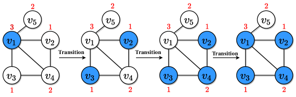
Figure 1: The evolution of a $(\textsc{Bool},\textsc{Thresh})$-SyDS $\mathcal{S}=(G_{\mathcal{S}}{},\mathcal{F})$ where $V(G_{\mathcal{S}}{})=\{v_{i}:i=1,...,5\}$. The threshold values are shown in red: $\tau_{1}=3,\tau_{2}=1,\tau_{3}=1,\tau_{4}=2,$ and $\tau_{5}=2$. State-1 nodes are highlighted in blue. The system undergoes the following evolution: $(1,0,0,0,0)\rightarrow(0,1,1,0,0)\rightarrow(0,1,1,1,0)\rightarrow(1,1,1,1,0)$, with the last configuration being a fixed point.

Constant-state nodes.

A node $v\in V$ is a constant-1 node if $\tau_{v}=0$, that is, given any configuration $C$, the state of $v$ is 1 in the successor $C^{\prime}$ of $C$. Similarly, $v$ is a constant-0 node if $\tau_{v}=deg(v)+2$.

3.1 Problem definition

Let $\mathcal{S}=(G_{\mathcal{S}}{},\mathcal{F})$ be a SyDS and let $C$ be a configuration of $\mathcal{S}$. The Hamming weight of $C$, denoted by $H(C)$, is the number of $1$’s in $C$. A minimum fixed point of $\mathcal{S}$ is a fixed point with the smallest possible Hamming weight. Note that when a $(\textsc{Bool},\textsc{Thresh})$-SyDS $\mathcal{S}$ has no constant-1 nodes, the minimum fixed point of $\mathcal{S}$ is trivially $\textbf{0}^{n}$. A nontrivial fixed point is a fixed point that is different from $\textbf{0}^{n}$. Our work focuses on finding nontrivial minimum fixed points.

Definition 3.1.

A nontrivial minimum fixed point of $\mathcal{S}$ is a nontrivial fixed point of minimum Hamming weight.

We now provide a formal definition of the problem.

Nontrivial Minimum Fixed Point Existence (NMin-FPE)

Instance: A SyDS $\mathcal{S}=(G_{\mathcal{S}}{},\mathcal{F})$ and a positive integer $q$.

Question: Is there a fixed point $C$ of $\mathcal{S}$ with Hamming weight at least $1$ and at most $q$?

We focus on the NP-optimization version of NMin-FPE which is to find a nontrivial minimum fixed point.

4 Computational Hardness of NMIN-FPE

In this section, we present an inapproximability result for NMin-FPE. Specifically, we show that NMin-FPE cannot be poly-time approximated within a factor $n^{1-\epsilon}$ for any constant $\epsilon>0$, unless $\textbf{P}=\textbf{NP}$. We also establish that NMin-FPE is W[1]-hard, with the parameter being the Hamming weight of a fixed point. Under standard hypotheses in computational complexity, our results rule out the possibility of obtaining efficient approximation algorithms with provable performance guarantees and fixed parameter tractable algorithms w.r.t. the Hamming weight for NMin-FPE.

Theorem 4.1.

The problem NMin-FPE cannot be approximated to within a factor $n^{1-\epsilon}$ for any constant $\epsilon>0$, unless $\textbf{P}=\textbf{NP}$. This inapproximability holds even when the underlying graph is bipartite.

Proof.

We first consider the case where $0<\epsilon<1$. The overall scheme of our proof is a reduction from minimum vertex cover to NMin-FPE such that if there exists a poly-time factor $n^{1-\epsilon}$ approximation algorithm $\mathcal{A}$ for NMin-FPE, we then can use $\mathcal{A}$ to solve the Minimum vertex cover problem in polynomial time, implying $\textbf{P}=\textbf{NP}$. Let $\mathcal{M}=\langle G_{\mathcal{M}},k\rangle$ be an arbitrary instance of Minimum vertex cover (MVC) with target size $k$, where $n_{\mathcal{M}}=|V(G_{\mathcal{M}})|$ and $m_{\mathcal{M}}=|E(G_{\mathcal{M}})|$. Without loss of generality, we assume that $G_{\mathcal{M}}$ is connected. Moreover, observe when $k=n_{\mathcal{M}}-1$, MVC can be solved in polynomial time. Therefore, we assume that $k<n_{\mathcal{M}}-1$.

Let $\mathcal{A}$ be a polynomial time factor $n^{1-\epsilon}$ approximation algorithm for NMin-FPE, $0<\epsilon<1$, where $n$ is the number of vertices in the underlying graph. We build an instance $\mathcal{S}=(G_{\mathcal{S}}{},\mathcal{F})$ of NMin-FPE for which $n_{\mathcal{S}}=|V(G_{\mathcal{S}}{})|$ and $m_{\mathcal{S}}=|E(G_{\mathcal{S}}{})|$. Let $\alpha=m_{\mathcal{M}}+n_{\mathcal{M}}+1$, and $\beta=\alpha^{\lceil 2/\epsilon\rceil}$. The construction is as follows.

1. The vertex set $V(G_{\mathcal{S}})$. Let $X=\{x_{u}:u\in V(G_{\mathcal{M}})\}$ and $Y=\{y_{e}:e\in E(G_{\mathcal{M}})\}$ be two sets of vertices that corresponds to vertices and edges in $G_{\mathcal{M}}$, respectively. Let $w,z$ be two additional vertices. Lastly, we introduce a set of $\beta$ vertices $R=\{r_{1},...,r_{\beta}\}$. Then $V(G_{\mathcal{S}})=X\cup Y\cup R\cup\{w\}\cup\{z\}$.

   We use notations $x_{u}\in X$, $y_{e}\in Y$, $r_{i}\in R$, $w$ and $z$ and to distinguish the five classes of vertices in $G_{\mathcal{S}}$.

2. The edge set $E(G_{\mathcal{S}})$. Let $E_{1}=\{(x_{u},y_{e}):$ $u\in V(G_{\mathcal{M}})$ is incident to $e\in E(G_{\mathcal{M}})\}$ be the edge set such that if a vertex $u$ and an edge $e$ are incident in $G_{\mathcal{M}}$, their corresponding vertices $x_{u}$ and $y_{e}$ are adjacent in $G_{\mathcal{S}}$. Let $E_{2}=\{(y_{e},z):y_{e}\in Y\}$ be the edge set where vertex $z$ is adjacent to all $y_{e}\in Y$. Let $E_{3}=\{(x_{u},w):x_{u}\in X\}$ be the edge set such that $w$ is adjacent to all $x_{u}\in X$. Let $E_{4}=\{(r_{i},r_{i+1}):r_{i}\in R,1\leq i\leq\beta-1\}$, that is, vertices in $R$ form a path. Lastly, we introduce an additional edge $(w,r_{1})$ to connect $w$ with an endpoint of the above path. The edge set of $G_{\mathcal{S}}$ is then defined as $E(G_{\mathcal{S}}{})=\bigcup_{i=1}^{4}E_{i}\cup\{(w,r_{1})\}$.

3. Thresholds. The threshold $\tau_{x_{u}}$ of each $x_{u}\in X$ is $deg(u)+1$ where $deg(u)$ is the degree of vertex $u$ in $G_{\mathcal{M}}$. The thresholds $\tau_{y_{e}}$ of all $y_{e}\in Y$ is $3$. The thresholds of $w$ and $z$ are $k+1$ and $m_{\mathcal{M}}+1$, respectively. Lastly, all $r_{i}\in R$ have threshold $1$.

This completes the construction of the NMin-FPE instance $\mathcal{S}=(G_{\mathcal{S}},\mathcal{F})$ which clearly takes polynomial time w.r.t. $n_{\mathcal{M}}$. The resulting graph $G_{\mathcal{S}}{}$ has $n_{\mathcal{S}}=n_{\mathcal{M}}+m_{\mathcal{M}}+\beta+2$ vertices and $m_{\mathcal{S}}=n_{\mathcal{M}}+3m_{\mathcal{M}}+\beta$ edges. Furthermore, $G_{\mathcal{S}}{}$ is bipartite. An example of reduction is shown in Figure 2. We now argue that $G_{\mathcal{M}}$ has a vertex cover of size at most $k$ if and only if the algorithm $\mathcal{A}$ returns a non-zero fixed point of size at most $n_{\mathcal{S}}^{1-\epsilon}\alpha$ where $\alpha=m_{\mathcal{M}}+n_{\mathcal{M}}+1$.

• Let $V^{\prime}\subseteq V(G_{\mathcal{M}})$ be a vertex cover of size $k$. We can construct a fixed point $I$ of $\mathcal{S}$ by setting (1) the states of all $y_{e}\in Y$ to $1$, (2) for all $u\in V^{\prime}$, the states of $x_{u}\in X$ to $1$, and (3) the state of vertex $z$ to 1. The number of 1’s in the resulting configuration $I$ is $m_{\mathcal{M}}+k+1$. We now show that $I$ is a fixed point. Let $I^{\prime}$ be the successor of $I$. It is easy to see that the state of vertices in $R\cup\{w\}$ remains $0$ and state of $z$ remains 1 in $I^{\prime}$. We consider the following two cases of the state of a vertex $x_{u}\in X$ under $I$. If the state of $x_{u}$ is 1, then since all $y_{e}$’s have state $1$, the input to $x_{u}$’s local function is $deg(x_{u})+1=\tau_{x_{u}}$. Thus, $x_{u}$ remains in state $1$ under $I^{\prime}$. If the state of $x_{u}$ is $0$ under $I$, the input to $x_{u}$’s local function is $deg(x_{u})<\tau_{x_{u}}$ and $x_{u}$ remains in state $0$ under $I^{\prime}$. It follows that $I$ is a fixed point.

  Let $\textsc{OPT}(\mathcal{S})$ denote the Hamming weight of a nontrivial minimum fixed point of $\mathcal{S}$ which is at most $k+m_{\mathcal{M}}+1$ Let $C$ be a fixed point returned by algorithm $\mathcal{A}$. Since $\mathcal{A}$ have an approximation factor of $n^{1-\epsilon}$, we have

  $$H(C)\leq n_{\mathcal{S}}^{1-\epsilon}\cdot\textsc{OPT}\leq n_{\mathcal{S}}^{1-\epsilon}\cdot(k+m_{\mathcal{M}}+1)\leq n_{\mathcal{S}}^{1-\epsilon}\cdot\alpha$$ (1)

• We prove the contrapositive. Suppose $G_{\mathcal{M}}$ does not have a vertex cover of size at most $k$, we establish the following two claims.

  Claim 3.1.1.

  Under any fixed point $C$ of $\mathcal{S}$ where the vertex $w$ is in state $0$, there exists a state-1 vertex in $X\cup Y\cup\{z\}$ if and only if all $y_{e}\in Y$’s have state $1$ under $C$.

  The necessity of the claim clearly holds. We prove the contrapositive of the other direction. Suppose there exists a vertex $y_{e}\in Y$ with state $0$ under $C$, let $x_{u}$ and $x_{v}$ be the two neighbors of $y_{e}$. Observe $x_{u}$ and $x_{v}$ must have state $0$ since their thresholds are degrees plus one. Similarly, the vertex $z$ also has state $0$ under $C$. As a result, all neighbors of $x_{u}$ and $x_{v}$ have state $0$. By recursion, all vertices in $X\cup Y\cup\{z\}$ have state $0$ under $C$. This concludes the claim.

  Claim 3.1.2.

  For any non-zero fixed point $C$ of $\mathcal{S}$, all vertices in $R$ must have state $1$ under $C$.

  Suppose there exists a non-zero fixed point $C$ where at least one vertex $r_{i}\in R$ has state $0$. Since $\tau_{r_{i}}=1,\;\forall r_{i}\in R$, it follows that all vertices in $R$ and vertex $w$ must have state $0$ under $C$. We now consider the states of other vertices under $C$. Given the $\tau_{w}=k+1$, the number of state-$1$ vertices in $X$ is at most $k$. Note that however, since $G_{\mathcal{M}}$ does not have a vertex cover of size $k$, under any combinations of $k$ state-$1$ vertices in $X$, there exists at least one vertex $y_{e}\in Y$ such that both $y_{e}$’s neighbors in $X$ have state $0$ under $C$. Since $\tau_{y_{e}}=3,\;\forall y_{e}\in Y$, there must exist a vertex $y_{e}\in Y$ with state $0$ under $C$. Follows from the Claim 3.1.1, $C$ is a zero fixed point which yields the contraposition. This concludes the proof of the claim.

  By the claim above, we have $\textsc{OPT}(\mathcal{S})\geq\beta=\alpha^{\lceil 2/\epsilon\rceil}$. We now argue that $n_{\mathcal{S}}^{1-\epsilon}\cdot\alpha<\alpha^{\lceil 2/\epsilon\rceil}$. Let $\lambda=\lceil 2/\epsilon\rceil-2/\epsilon$, we then rewrite $n_{\mathcal{S}}^{1-\epsilon}\cdot\alpha$ as

  $$n_{\mathcal{S}}^{1-\epsilon}\cdot\alpha=(\alpha^{\frac{2}{\epsilon}+\lambda}+\alpha+1)^{1-\epsilon}\cdot\alpha$$ (2)

  where $n_{\mathcal{S}}=n_{\mathcal{M}}+m_{\mathcal{M}}+\beta+2=\alpha+\alpha^{\lceil 2/\epsilon\rceil}+1$. Since $n_{\mathcal{M}}\geq 1$ and $0\leq\epsilon<1$, we have $\alpha\geq 2$ and $2/\epsilon+\lambda=\lceil 2/\epsilon\rceil\geq 3$. Thus,

  $$\alpha+1<\alpha^{\frac{2}{\epsilon}+\lambda}\leq(\alpha-1)\cdot\alpha^{\frac{2}{\epsilon}+\lambda}$$ (3)

  and it follows that

  $$\alpha^{\frac{2}{\epsilon}+\lambda}+\alpha+1<\alpha^{\frac{2}{\epsilon}+\lambda+1}$$ (4)

  Since $1-\epsilon>0$,

  $$(\alpha^{\frac{2}{\epsilon}+\lambda}+\alpha+1)^{1-\epsilon}\cdot\alpha <(\alpha^{\frac{2}{\epsilon}+\lambda+1})^{1-\epsilon}\alpha$$

  $$=\alpha^{(\frac{2}{\epsilon}+\lambda+1)(1-\epsilon)+1}$$

  $$=\alpha^{\lceil\frac{2}{\epsilon}\rceil-\epsilon\lambda-\epsilon}$$

  $$<\alpha^{\lceil\frac{2}{\epsilon}\rceil}$$

  Overall, we have $n_{\mathcal{S}}^{1-\epsilon}\cdot\alpha<\alpha^{\lceil 2/\epsilon\rceil}\leq\textsc{OPT}(\mathcal{S})$. Let $C$ be the non-zero fixed point returned by $\mathcal{A}$. It follows immediately that $H(C)>n_{\mathcal{S}}^{1-\epsilon}\cdot\alpha$.

Since $n_{\mathcal{S}}=n_{\mathcal{M}}+m_{\mathcal{M}}+\beta+1$ is polynomial w.r.t. $n_{\mathcal{M}}$, the algorithm $\mathcal{A}$ runs in polynomial time w.r.t. $n_{\mathcal{M}}$. The reduction implies that if there exists such an algorithm $\mathcal{A}$ with approximation factor $n^{1-\epsilon}$ for any constant $0<\epsilon<1$, based on the Hamming weight of the fixed point returned by $\mathcal{A}$, we can solve MVC in polynomial time, implying $\textbf{P}=\textbf{NP}$. For the case where $\epsilon\geq 1$, note that the resulting approximation factor $n^{1-\epsilon}$ is less than any factor when $0<\epsilon<1$, thus, the inapproximability follows immediately. Overall, we conclude that NMin-FPE cannot be approximated within a factor $n^{1-\epsilon}$ for any constant $\epsilon>0$, unless $\textbf{P}=\textbf{NP}$, and the hardness holds even when the underlying graph is bipartite. ∎

Figure 2: An example of the reduction from MVC to NMin-FPE where $G_{\mathcal{M}}$ and $G_{\mathcal{S}}$ are graphs for MVC and NMin-FPE, respectively.

Theorem (4.1) establishes a strong inapproximability result for NMin-FPE; it points out that even obtaining an approximation guarantee that is slightly better than a linear factor is hard.

Parameterized Complexity of NMIN-FPE.

Next, we examine whether NMin-FPE is fixed-parameter tractable (FPT) w.r.t. a natural structural parameter of the problem, namely the Hamming weight of a fixed point.

Theorem 4.2.

The problem NMin-FPE is W[1]-hard w.r.t. to the natural parameter (i.e., the Hamming weight of a fixed point) for (Bool, Thresh)-SyDSs.

Proof.

We give a parameterized reduction from the Clique problem to NMin-FPE. Let $\langle G_{\mathcal{C}},k\rangle$ be an arbitrary instance of the clique problem, we construct a NMin-FPE instance $\langle\mathcal{S}=(G_{\mathcal{S}},\mathcal{F}),q\rangle$ by generating a subdivision of $G_{\mathcal{C}}$. In particular, each edge $e=(u,v)\in E(G_{\mathcal{C}})$ is transformed into two edges $(x_{u},y_{e})$ and $(y_{e},x_{v})$ in $E(G_{\mathcal{S}})$, where (1) $x_{u},x_{v}\in V(G_{\mathcal{S}})$ correspond to the vertices $u,v\in V(G_{\mathcal{C}})$, respectively, and (2) $y_{e}\in V(G_{\mathcal{S}})$ corresponds to the edge $e\in E(G_{\mathcal{C}})$. For clarity, we use $X=\{x_{u}:u\in V(G_{\mathcal{C}})\}$ and $Y=\{y_{e}:e\in E(G_{\mathcal{C}})\}$ to denote the sets of two types of vertices in $G_{\mathcal{S}}$ that correspond to vertices and edges in $G_{\mathcal{C}}$, respectively. Subsequently, $V(G_{\mathcal{S}})=X\cup Y$. The threshold of each $y_{e}\in Y,e\in E(G_{\mathcal{C}})$ is $3$, and the threshold value of each $x_{u}\in X,u\in V(G_{\mathcal{C}})$ is $k$. Lastly, we set $q=k+k(k-1)/2=k(k+1)/2$. This completes the construction of the NMin-FPE instant. An example reduction is shown in Figure 3. To see that this is a parameterized reduction, we remark that the reduction can be carried out in $O(|V(G_{\mathcal{C}})+E(G_{\mathcal{C}})|)$ time, which is fixed parameter tractable w.r.t. $k$. Furthermore, we have $q<k^{3}$.

We now claim that there is a clique of size $k$ in $G_{\mathcal{C}}$ if and only if $\mathcal{S}$ has a fixed point $C$ with Hamming weight $1\leq H(C)\leq q$.

• Let $V^{\prime}\subseteq V(G_{\mathcal{C}})$ be the subset of vertices that form a $k$-clique in $G_{\mathcal{C}}$. We construct a fixed point $C$ of $\mathcal{S}$ by first setting vertices $x_{u}\in X,\forall u\in V^{\prime}$ to state $1$. Furthermore, for each edge $e=(u,v)\in E(G_{\mathcal{C}})$ where $u,v\in V^{\prime}$, we set the vertex $y_{e}\in Y$, which is the vertex that corresponds to $e$, to state $1$. All other vertices in $V(G_{\mathcal{S}})$ are set to state $0$ under $C$. Note that the number of state-$1$ vertices in $X$ are $Y$ is $k$ and $k(k-1)/2$, respectively, thus, we have $H(C)=k+k(k-1)/2=k(k+1)/2=q$.

  We now claim that $C$ is a fixed point. Let $C^{\prime}$ be the successor of $C$. We first consider each vertex $x_{u}\in X$. If the state of $x_{u}$ is $1$ under $C$, then we have $u\in V^{\prime}$ and by the construction above, $x_{u}$ has exactly $k-1$ neighbors in state $1$. Thus, $\tau_{u}$ is satisfied and $x_{u}$ remains state $1$ under $C^{\prime}$. On the other hand, if $x_{u}$ is in state $0$, then $u$ is not in the $k$ clique of $G_{\mathcal{C}}$, and $x_{u}$ would have no neighbors in state $1$ under $C$. Thus, the state of $x_{u}$ remains $0$ in $C^{\prime}$. A similar argument can be made for each vertex $y_{e}\in V(G_{\mathcal{S}})$. Overall, we conclude that $C$ is a fixed point.

• We first prove the following claim.

  Claim 3.2.1.

  Any non-zero fixed point $C$ of $\mathcal{S}$ has Hamming weight at least $q=k(k+1)/2$.

  Let $x_{u}\in X$ be a state-1 vertex under $C$. Since the threshold of $x_{u}$ is $k$, at least $k-1$ of its neighbors are in state $1$. Let $y_{e}$ be a state-1 neighbor of $x_{u}$. Given that the threshold value of $y_{e}$ is $3$, both of its neighbors should also be in state $1$ under $C$. Therefore, under any non-zero fixed point, the number of $x_{u}\in X$ in state $1$ is at least $k$ and the number of $y_{e}\in Y$ in state 1 is at least $k(k-1)/2$. Thus, the Hamming weight of $C$ is at least $k(k+1)/2$. This concludes the claim.

  Now suppose there exists a fixed point $C$ with $1\leq H(C)\leq q$, by the claim above, we must have $H(C)=q$. Note that the equality in the claim 3.2.1 holds only when the number of state-1 $x_{u}\in V(G_{\mathcal{S}})$ is exactly $k$ and the number of state-1 $y_{e}\in V(G_{\mathcal{S}})$ is exactly $k(k-1)/2$, that is, the set of vertices $\{u\in V(G_{\mathcal{C}}),\text{$x_{u}$ is in state-1 under $C$}\}$ form a $k$ clique of $G_{\mathcal{C}}$.

Since clique is W[1]-hard w.r.t. the natural parameter $k$, the theorem follows immediately. ∎

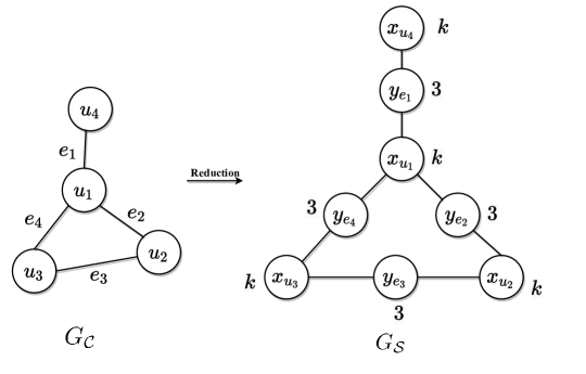
Figure 3: An example of the W[1]-hardness reduction from Clique to NMin-FPE where $G_{\mathcal{C}}$ and $G_{\mathcal{S}}$ are graphs for Clique and NMin-FPE, respectively. Threshold values are placed next to vertices in $G_{\mathcal{S}}$

Theorem (4.2) implies that NMin-FPE is not FPT w.r.t. to the natural parameter. Note that this does not exclude FPT results for other parameters, as we identify one such parameter in the next section.

5 Approaches for Solving NMIN-FPE

In this section, we consider several approaches for tackling the hardness of NMin-FPE. We start by identifying special cases where the problem can be solved efficiently. We also present an integer linear programming (ILP) formulation that can be used to obtain optimal solutions for networks of reasonable sizes. Then we introduce a heuristic framework for NMin-FPE that is useful in obtaining good (but not necessarily optimal) solutions in larger networks.

5.1 Efficient algorithms for special classes

Restricted classes.

We identify four special classes of problem instances where NMin-FPE can be solved in polynomial time. Motivated by real-world scenarios, we consider the classic progressive threshold model [18], where once a vertex changes to state $1$, it retains the state $1$ for all subsequent time-steps. We also investigate special graph classes such as directed acyclic graphs and complete graphs.

Observation 5.1.

Let $\mathcal{S}$ be a $(\textsc{Bool},\textsc{Thresh})$-SyDS. Given two configurations $C_{1}$ and $C_{2}$ of $\mathcal{S}$, let $C_{1}^{\prime}$ and $C_{2}^{\prime}$ be the successors of $C_{1}$ and $C_{2}$, respectively. If $C_{1}\preceq C_{2}$, then $C_{1}^{\prime}\preceq C_{2}^{\prime}$.

Theorem 5.2.

4.1 For (Bool, Thresh)-SyDSs, NMin-FPE admits a polynomial time algorithm for any of the following restricted cases:

1. There exists at least one vertex with $\tau_{v}=0$.

2. The SyDS uses the progressive threshold model.

3. The underlying graph is a directed acyclic graph.

4. The underlying graph is a complete graph.

Proof.

Let $\mathcal{S}=(G_{\mathcal{S}}{},\mathcal{F})$ be an arbitrary (Bool, Thresh)-SyDS.

Claim 4.1.1.

If there exists a vertex $v$ with $\tau_{v}=0$, then NMin-FPE can be solved in $O(m+n)$ time.

Let $V^{\prime}=\{v\;:\;v\in V(G_{\mathcal{S}}),\tau_{v}=0\}$ be the subset of vertices with thresholds $0$. Let $C_{1}$ be the configuration that consists of all $0$’s. We consider the evolution of $\mathcal{S}$ from $C_{1}$. Let $C_{i}$ denote the successor of the configuration $C_{i-1}$, $i\geq 2$, that is, $C_{2}$ is the successor of $C_{1}$, $C_{3}$ is the successor of $C_{2}$, etc. Following from the observation 5.1, we have $C_{i}\preceq C_{i+1}$, $i\geq 1$. Since $G_{\mathcal{S}}$ has a finite number of vertices, by recursion, $\mathcal{S}$ must reach a fixed point, denoted by $C_{k}$, from $C_{1}$ in $O(n)$ transitions. The evolution of $\mathcal{S}$ from $C_{1}$ to $C_{k}$ can be seen as a BFS process which takes $O(m+n)$ time.

We now argue that $C_{k}$ is a nontrivial minimum fixed point of $\mathcal{S}$. It is easy to see that $C_{k}$ is non-zero since all vertices in $V^{\prime}$ must be in state $1$ under $C_{k}$. Furthermore, for any non-zero fixed point $C$, we have $C_{1}\preceq C$. Since $C$ is a fixed point, the successor of $C$ is $C$ itself. Thus, by the observation 5.1, we have $C_{i}\preceq C$, $1\leq i\leq k$. It follows that all state-1 vertices in $C_{k}$ are also in state $1$ under $C$, and $H(C_{k})\leq H(C)$. This concludes the claim 4.1.1.

For other cases below, we assume that $\tau_{v}>0,\forall v\in V(G_{\mathcal{S}})$ without losing generality.

Claim 4.1.2 .

Under the progressive threshold model, NMin-FPE can be solved in $O(mn+n^{2})$ time.

We label vertices in $V(G_{\mathcal{S}}{})$ from $v_{1}$ to $v_{n}$ arbitrarily. The algorithm consists of $n$ iterations. At the $i$th iteration, $1\leq i\leq n$, we construct an initial configuration $C_{i}$ by setting only vertex $v_{i}$ to state $1$, and all other vertices to state $0$. We then evolve the system from $C_{i}$ which always reaches to some fixed point $C_{i}^{*}$ in $O(n)$ time-step, since no vertices can flip from state $0$ back to state $1$. By repeating the above process for $n$ iterations, we get a collection of $n$ fixed points $\mathcal{I}=\{C^{*}_{1},C^{*}_{2},...,C^{*}_{n}\}$ (they are not necessarily unique). Because of the progressive model, all $n$ fixed points are non-zero. We remark that a fixed point with minimum Hamming weight in $\mathcal{I}$ is a nontrivial minimum fixed point of the system, denoted by $C^{*}$. To see this, note that given any non-zero fixed point $C$ of $\mathcal{S}$, if the state of some $v_{i}\in V(G_{\mathcal{S}})$ is $1$ under $C$, then all state-$1$ vertices in $C^{*}_{i}$ must also be in state $1$ under $C$, thus, $H(C)\geq H(C_{i}^{*})\geq H(C^{*})$.

As of running time, each iteration involves a full evolution of $\mathcal{S}$ from an initial configuration to a fixed point which can be seen as a BFS process taking $O(m+n)$ time. Thus, the overall running time is $O(mn+n^{2})$. We remark that if $G_{\mathcal{S}}$ is connected, then the running time is $O(mn)$. This concludes the proof of the Claim 4.1.2.

Claim 4.1.3.

NMin-FPE can be solved in $O(mn+n^{2})$ time for $\mathcal{S}$ when $G_{\mathcal{S}}$ is a directed acyclic graph.

We first establish that if all vertices have thresholds greater than $1$, then $\mathcal{S}$ has no valid nontrivial minimum fixed point (In particular, the only fixed point of the system is the configuration that consists of all $0$’s). Given any fixed point $C$ of $\mathcal{S}$, let $v_{1}\in V(G_{\mathcal{S}})$ be a vertex with $0$ in-degree. Note that such a vertex $v_{1}$ must exist, or else, $G_{\mathcal{S}}$ has at least one directed cycle. Since $\tau_{v_{1}}\geq 2>d^{-}_{v_{1}}+1$ where $d^{-}_{v}=0$ is the in-degree of $v_{1}$, the state of $v_{1}$ is $0$ under $C$, and the input from $v_{1}$ to any one of its out-neighbors’ local functions is $0$. Thus, we can only consider the subgraph induced on $V(G_{\mathcal{S}})\setminus\{v_{1}\}$. Note that the resulting subgraph is also acyclic. Let $v_{2}\in V(G_{\mathcal{S}})\setminus\{v_{1}\}$ be the next vertex with $0$ in-degree. Similarly, $v_{2}$ must also have state $0$ under $C$. By recursion, we conclude that all vertices have state $0$ under $C$ if all vertices have thresholds greater than $1$.

Suppose there exists at least one vertex with a threshold equals to $1$ (we have assumed that no vertices have threshold $0$) in $\mathcal{S}$. The algorithm in finding a nontrivial minimum fixed point is shown in Algorithm 1. We now prove its correctness. Let $C$ be any non-zero fixed point of $\mathcal{S}$. We claim that among all the vertices with state $1$ under $C$, one of them must have a threshold equal to $1$. For contradiction, suppose all the state-$1$ vertices have thresholds at least $2$. This implies that each state-$1$ vertex must have an in-neighbor who also has state $1$ under $C$. Since the graph is finite, the state-1 vertices form a cycle which contradicts $G_{\mathcal{S}}$ being acyclic. Thus, any non-zero fixed point $C$ of $\mathcal{S}$ must contain at least one state-$1$ vertex with a threshold equal to $1$. Let $v$ denote such a vertex, we then have $H(C)\leq H(C^{*}_{v})$, where $C^{*}_{v}$ is the fixed point reach from the initial configuration with only $v$ being in state $1$. The correctness of the algorithm follows immediately. Lastly, a full evolution of $\mathcal{S}$ from an initial configuration to a fixed point can be treated as a BFS process which takes $O(m+n)$ time, thus, the running time of the algorithm is $O(mn+n^{2})$.

Claim 4.1.4.

NMin-FPE can be solved in $O(n^{2}+m)$ time for $\mathcal{S}$ when $G_{\mathcal{S}}$ is a complete graph.

Let $q$ be the number of distinct threshold values in $\mathcal{S}$. We partition the vertex set $V(G_{\mathcal{S}})$ into $q$ non-empty subsets $P=\{V_{1},...,V_{p}\}$, such that two vertices have the same threshold if and only if they are in the same subset $V_{i}$, $1\leq i\leq q$. Moreover, subsets are in ascending order by thresholds, that is, $\tau_{u}<\tau_{v}$ if and only if $u\in V_{i}$, $v\in V_{j}$ and $1\leq i<j\leq q$. Given that $G_{\mathcal{S}}$ is a complete graph, we make the following key observations. First, under a configuration $C$, the number of state-$1$ vertices in the closed neighborhood of each vertex is $H(C)$. Second, if $C$ is a fixed point and a vertex $u\in V_{i}$, $1\leq i\leq q$ is in state $1$, then all vertices in the subsets $V_{1},...,V_{i}$ must be in state $1$.

Under a configuration $C$, we call a state-$1$ vertex $v$ unsatisfied if the number of state-$1$ vertices in $v$’s closed neighborhood is less than $\tau_{v}$, that is, $H(C)<\tau_{v}$. Overall, the algorithm starts with a configuration $I$ of all $0$’s and iteratively sets vertices to state $1$ until a there are no unsatisfied vertices. Specifically, at an iteration of the algorithm, let $V^{\prime}$ be the subset of unsatisfied vertices under $I$, and let $\tau^{\prime}$ denote the smallest threshold among all state-$0$ neighbors of vertices in $V^{\prime}$. We set the states of all vertices with thresholds at most $\tau^{\prime}$ to $1$ under $I$ and repeat the process until $V^{\prime}$ is an empty set. The detailed pseudocode is given in Algorithm 2. The while loop (line 5) in Algorithm 2 consists of at most $n$ iterations. The for loop from line 6 to 10 takes $O(n)$ time since we never set the same vertex to state $1$ twice. Furthermore, all other operations from line 11 to 15 take $O(n)$ time. Given that the system evolution at line $17$ takes $O(m+n)$ time, the running time of the Algorithm 2 is $O(n^{2}+m)$.

We now claim the correctness of the algorithm. Consider the configuration $I$ (defined in the pseudocode) after the termination of the while loop in the algorithm 2. It is easy to see that the thresholds of all state-$1$ vertices are satisfied under $I$. Follows from the monotonicity of threshold functions, $\mathcal{S}$ evolving from $I$ will always reach a non-zero fixed point $I^{*}$.

We argue that $I^{*}$ is minimum. Let $C$ be any non-zero fixed point, and let $\tau_{C}=\max\{\tau_{v}\;|\;\forall v\in V(G_{\mathcal{S}}{}),C(v)=1\}$ be the largest threshold over all state-$1$ vertices under $C$. Moreover, let $\tau_{I}=\max\{\tau_{v}\;|\;\forall v\in V(G_{\mathcal{S}}{}),I(v)=1\}$ be the largest threshold over all state-$1$ vertices under $I$. We must have $\tau_{I}\leq\tau_{C}$. For contradiction, suppose $\tau_{I}>\tau_{C}$. Let $V_{j}\in P$ be the subset in the partition where $\tau_{v}=\tau_{C},\forall v\in V_{j}$. Follows from $C$ being a fixed point, the while loop would have terminated when the states of all vertices in $V_{j}$ are set to one under $I$, implying that $\tau_{I}=\tau_{C}$ which yields a contradiction. It follows that $\tau_{I}\leq\tau_{C}$. Since $G_{\mathcal{S}}{}$ is a complete graph, in any non-zero fixed point of $\mathcal{S}$, if $v\in V(G_{\mathcal{S}}{})$ has state $1$, then all vertices $u$ with $\tau_{u}\leq\tau_{v}$ are in state $1$. Subsequently, all state-$1$ vertices in $I$ are also in state $1$ under $C$. It follows immediately that all state-$1$ vertices in $I^{*}$ are also in state $1$ under $C$, implying $H(I^{*})\leq H(C)$. This concludes the claim 4.1.4. ∎

Input : A (Bool, Thresh)-SyDS $\mathcal{S}$ = $(G_{\mathcal{S}},\mathcal{F})$ where $G_{\mathcal{S}}$ is a dag.

1

Output : A non-trivial minimum fixed point $C^{*}$

2

3$V^{\prime}=\{v:v\in V(G_{\mathcal{S}}),\tau_{v}=1\}$

4

5$min\_h=|V(G_{\mathcal{S}})|+1$

6

7for each $v\in V^{\prime}$ do

8        $C_{v}\leftarrow$ the configuration where only $v$ is in state $1$

9       

10       $C^{*}_{v}\leftarrow$ the fixed point of $\mathcal{S}$ reached from $C_{v}$

11       

12       if $H(C^{*}_{v})<min\_h$ then

13               $min\_h=H(C^{*}_{v})$

14              

15              $C^{*}=C^{*}_{v}$

16              

17        end if

18       

19 end for

20return $C^{*}$

21

Algorithm 1 NMin-FPE_DAG($\mathcal{S}$)

Input : A (Bool, Thresh)-SyDS $\mathcal{S}=(G_{\mathcal{S}},\mathcal{F})$; $G_{\mathcal{S}}$ is a complete graph

1

Output : A non-trivial minimum fixed point $C^{*}$

2

3$P\leftarrow\{V_{1},V_{2},...,V_{p}\}:$ a partition of $V(G_{\mathcal{S}})$ such that two vertices have the same threshold iff they are in the same subset, and $\tau_{u}<\tau_{v}$ iff $u\in V_{i}$, $v\in V_{j}$ and $1\leq i<j\leq 1$.

4

5$V^{\prime}\leftarrow V_{1}$

6

7$I\leftarrow$ a configuration that consists of all zeros

8

9$j=k=1$

10

11while $V^{\prime}\neq\emptyset$ do

12        for $i$ from $j$ to $k$ do

13               for $v\in V_{i}$ do

14                      $I(v)=1$ $\triangleright$ Change the state of $v$ to $1$ under $I$

15               end for

16              

17        end for

18       

19       $V^{\prime}=\{v\in\bigcup_{l=1}^{k}V_{l}\;:\;H(I)<\tau_{v}\}$

20       $N^{\prime}=\{u:\exists v\in V^{\prime},(u,v)\in E(G_{\mathcal{S}}),u\notin\bigcup_{l=1}^{k}V_{l}\}$

21       

22       $\tau^{\prime}=\min\{\tau_{u}\;|\;u\in N^{\prime}\}$

23       

24       $j=k+1$

25       

26       $k=$ index of the subset $V_{k}\in P$ where $\tau_{v}=\tau^{\prime},\forall v\in V_{k}$

27       

28 end while

29

30$I^{*}\leftarrow$ the fixed point of $\mathcal{S}$, evolved from $I$

31

32return $I^{*}$

Algorithm 2 NMin-FPE_complete_graphs($\mathcal{S}$)

Fixed parameter tractability.

We further extend the solvability of NMin-FPE and establish that NMin-FPE is fixed parameter tractable w.r.t. the number of nodes with thresholds greater than $1$. Specifically, we develop a quadratic kernelization algorithm that finds a nontrivial minimum fixed point in time $O(2^{k}+n+m)$.

Theorem 5.3.

For (Bool, Thresh)-SyDSs, NMin-FPE is fixed parameter tractable w.r.t. the parameter $k$ which is the number of nodes with thresholds greater than $1$.

Proof.

Given an instance $\mathcal{S}=(G_{\mathcal{S}}{},\mathcal{F})$ of NMin-FPE, let $k$ be the number of vertices with thresholds greater than $1$. We present an algorithm for finding a nontrivial minimum fixed point of $\mathcal{S}$ that runs in fpt-time w.r.t. $k$.

Let $\mathcal{P}=\{CC_{1},CC_{2},...CC_{l}\}$ be the collection of subsets of vertices with thresholds equal to $1$, such that each subset $CC_{i}\in\mathcal{P}$ forms a maximally connected components that consists of only threshold-$1$ vertices, where $l\geq 1$ is the number of such components. Observe that for each $CC_{i},1\leq i\leq l$, if one vertex in $CC_{i}$ has state $1$ under some fixed point $C$, then all vertices in $CC_{i}$ are in state $1$ under $C$ (with the possibility that some other vertices outside of $CC_{i}$ are also in state $1$). Let $I_{i}$ be the configuration where $I_{i}(v)=1$ iff $v\in CC_{i}$, that is, all vertices in $CC_{i}$ are in state $1$ and other vertices are in state $0$ under $I_{i}$. By the monotonicity of the threshold function, $\mathcal{S}$ evolving from $I_{i}$ must reach a fixed point, denoted by $C_{i}$, $1\leq i\leq l$. Subsequently, we have a collection $\{C_{1},C_{2},...,C_{l}\}$ of fixed points (not necessarily unique) where each $C_{i}$ corresponds a fixed point reached from the initial configuration $I_{i}$, $1\leq i\leq l$. We remark that for any fixed point $C$, if there exists a vertex $v\in CC_{i}$, $1\leq i\leq l$, with state $1$ under $C$, then $H(C)\geq H(C_{i})$ where equality holds only when $C=C_{i}$.

Now consider a nontrivial minimum fixed point $C^{*}$ of $\mathcal{S}$. Let $V^{*}=\{v\in V(G_{\mathcal{S}}{}):C^{*}(v)=1\}$ be the set of state-$1$ vertices under $C^{*}$. We distinguish between two cases, either (1) $\exists CC_{i}\in\mathcal{P}$, s.t. $V^{*}\cap CC_{i}\neq\emptyset$, or (2) $\forall CC_{i}\in\mathcal{P}$, s.t. $V^{*}\cap CC_{i}=\emptyset$. If $\exists CC_{i}\in\mathcal{P}$, $V^{*}\cap CC_{i}\neq\emptyset$, by our previous remark, $C^{*}=C_{i}$.

Now suppose that $\forall CC_{i}\in\mathcal{P}$, $V^{*}\cap CC_{i}=\emptyset$, that is, all state-$1$ vertices under $C^{*}$ have thresholds greater than $1$. We can then find such a $C^{*}$ by removing vertices with thresholds equal to $1$ in $G_{\mathcal{S}}{}$, leaving only the subgraph

$$G_{\mathcal{S}}{}^{\prime}=G_{\mathcal{S}}{}[V(G_{\mathcal{S}}{})\setminus\bigcup_{i=1}^{l}CC_{i}]$$

of $k$ vertices, where $G_{\mathcal{S}}{}[V(G_{\mathcal{S}}{})\setminus\bigcup_{i=1}^{l}CC_{i}]$ is the subgraph induced on $V(G_{\mathcal{S}}{})\setminus\bigcup_{i=1}^{l}CC_{i}$. Since thresholds of vertices in $CC_{i}$ $1\leq i\leq l$ are $1$, neighbors of vertices in $CC_{i}$ must have state $0$ under $C^{*}$. Therefore, to find an optimal solution $C^{*}$ within the subgraph $G_{\mathcal{S}}{}^{\prime}$, we need an additional constraint such that for each vertex $v\in V(G_{\mathcal{S}}{}^{\prime})$ that is adjacent to vertices in $CC_{i}$, $1\leq i\leq l$, $v$ must have state $0$.

Overall, our algorithm in finding a nontrivial minimum fixed point is as follows. First, we construct the collection $\mathcal{P}=\{CC_{1},CC_{2},....,CC_{i}\}$ of maximally connected component that consist of only threshold-$1$ vertices. Then, we compute the collection $\mathcal{Q}=\{C_{1},C_{2},...C_{l}\}$ of corresponding fixed points. Let $C^{\prime}=\operatorname*{arg\,min}\{H(C_{i}):C_{i}\in\mathcal{Q}\}$ be a fixed point in $\mathcal{Q}$ of the minimum Hamming weight. Next, we construct the subgraph $G_{\mathcal{S}}{}^{\prime}$ and enumerate over all fixed points restricted to $G_{\mathcal{S}}{}^{\prime}$ to find the an optimal fixed point, denoted by $C^{\prime\prime}$. Lastly, the algorithm returns $\operatorname*{arg\,min}\{H(C^{\prime}),H(C^{\prime\prime})\}$. The correctness of the algorithm follows immediately from our arguments above.

As of the running time, observe that $\mathcal{P}$, $\mathcal{Q}$ and $C^{\prime}$ can all be computed in $O(n+m)$ time. Moreover, since $|V(G_{\mathcal{S}}{}^{\prime})|=k$, $C^{\prime\prime}$ can be found in $O(2^{k})$ time. Thus, the overall running time is then $O(2^{k}+n+m)$, ftp w.r.t. $k$. This concludes the proof. ∎

5.2 Solving NMIN-FPE in general networks

We make the following assumptions without losing generality. As shown in Theorem 5.2, the problem NMin-FPE can be solved efficiently when constant-1 vertices are presented in the system. To tackle the hardness of the problem, we thus assume that there are no constant-1 vertices in the system. Furthermore, we assume that the underlying graph is connected. Lastly, one can determine in polynomial time whether the only fixed point of a threshold-SyDS is the trivial fixed point (by starting the system with all nodes set to state 1, and the evolve the system). Therefore, the proposed heuristic does not explicitly consider this case and we assume the system has at least one non-trivial fixed point.

An ILP formulation.

Given a (Bool, Thresh)-SyDS $\mathcal{S}=(G_{\mathcal{S}}{},\mathcal{F})$, our ILP solves the NMin-FPE problem by constructing a nonempty minimum-cardinality subset $V^{*}\subseteq V(G_{\mathcal{S}}{})$ of nodes to set to state $1$, and all nodes not in $V^{*}$ to state $0$, such that the resulting configuration is a fixed point of $\mathcal{S}$. Let $x_{v},\;v\in V(G_{\mathcal{S}}{})$, be a binary variable where $x_{v}=1$ if and only if node $v\in V^{*}$. Let $\Delta=max\_deg(G)+2$ denote a constant that is greater than the maximum degree of $G$. Let $N(v),\;v\in V(G_{\mathcal{S}}{})$ denote the closed neighborhood of $v$. Then an ILP formulation for NMin-FPE is defined as follows in (5). An optimal solution to the ILP yields a set of state-$1$ nodes in a nontrivial minimum fixed point.

$${\min} \sum_{v\in V(G_{\mathcal{S}}{})}x_{v}$$ (5a)

s.t. $$\tau_{v}x_{v}\leq\sum_{u\in N(v)}x_{u},\;\;\;\forall v\in V(G_{\mathcal{S}}{})$$ (5b)

$$\sum_{v\in V(G_{\mathcal{S}}{})}x_{v}\geq 1$$ (5c)

$$\Delta\cdot x_{v}+\tau_{v}\geq\sum_{u\in N(v)}x_{u}+1,\;\;\;\forall v\in V(G_{\mathcal{S}}{})$$ (5d)

$$x_{v}\in\{0,1\},\;\;\;\forall v\in V(G_{\mathcal{S}}{})$$ (5e)

Proof.

Under an optimal solution of the ILP, let $V^{*}=\{v\in V(G_{\mathcal{S}}{}):x_{v}=1\}$ be the subset of vertices $v$ whose variable $x_{v}$ is set to $1$. Let $C^{*}$ be the configuration where $C^{*}(v)=1$ if and only if $v\in V^{*}$. We now argue that $C^{*}$ is a fixed point. For a state-$1$ vertex $v$ under $C^{*}$, by the constraint (5b), the number of state-$1$ vertices in the closed neighborhood of $v$ is at least $\tau_{v}$, thus, $v$ is fixed at state $1$. For a vertex $v$ with state $0$, by constraint (5d), we have $\tau_{v}>\sum_{u\in N(v)}x_{u}$, that is, the number of state-$1$ vertices in the closed neighborhood is less than $\tau_{v}$ and the state of $v$ is fixed at $0$. Overall, we conclude that $C^{*}$ is a fixed point of $\mathcal{S}$. Since $V^{*}$ is minimum with $|V^{*}|\geq 1$, $C^{*}$ is a nontrivial minimum fixed point.

By a similar argument, given a nontrivial fixed point $C^{*}$ of $\mathcal{S}$, the vertex set $V^{*}=\{v\in V(G_{\mathcal{S}}{}):C^{*}(v)=1\}$ correspond to an optimal solution of the ILP that satisfies all the constraints. This concludes the proof. ∎

The greedy framework for heuristics.

As we have shown that NMin-FPE is hard to approximate, one can only rely on heuristics to quickly find solutions for large networks. Given a (Bool, Thresh)-SyDS $\mathcal{S}=(G_{\mathcal{S}}{},\mathcal{F})$, we propose a general framework that iteratively constructs a fixed point by greedily setting nodes to state $1$. Specifically, the framework iterates over each node $u\in V(G_{\mathcal{S}}{})$ and finds a fixed point seeded at $u$, which is denoted as $C_{u}$. In $C_{u}$, we have ($1$) $u$ is in state $1$, and ($2$) the Hamming weight of $C_{u}$ is heuristically the smallest. The algorithm then returns a fixed point $C_{u}$ with the smallest Hamming weight over all $u\in V(G_{\mathcal{S}}{})$ as shown in Algorithm 3.

Input : SyDS $\mathcal{S}=(G_{\mathcal{S}}{},\mathcal{F})$

Output : A fixed point $C^{*}\in\{0,1\}^{n}$

1 $best\_obj=|V(G_{\mathcal{S}}{})|$

2 for $u\in V(G)$ do

3        $C_{u}$ = Greedy_Seeded_NM1FPE$(\mathcal{S},\;u)$

4        if $H(C_{u})<best\_obj$ then

5               $best\_obj=H(C_{u})$

6              

7              $C^{*}=C_{u}$

8              

9        end if

10       

11 end for

12return $C^{*}$

13

Algorithm 3 NM1FPE$(\mathcal{S})$

We now introduce the greedy scheme to compute $C_{u},u\in V(G_{\mathcal{S}}{})$. Let $A_{u}\subseteq V(G_{\mathcal{S}}{})$ be a subset of state $1$ nodes under $C_{u}$. The scheme constructs $C_{u}$ by progressively adding nodes to $A_{u}$, which effectively set them to state $1$. Overall, the scheme has the following two key steps: (1) the construction of $A_{u}$ terminates when the fixed point condition is met. Specifically, ($i$) for each node $v\in A_{u}$, the threshold $\tau_{v}$ is satisfied, that is, the number of $v$’s neighbors (including $v$ itself) in $A_{u}$ is at least $\tau_{v}$, and ($ii$) for each node $v\in V(G_{\mathcal{S}}{})\setminus A_{u}$, the number of $v$’s neighbors in $A_{u}$ is less than $\tau_{v}$; (2) nodes are added to $A_{u}$ based on a greedy selection method specified by a heuristic. Under this framework, different heuristics can be obtained by using different greedy selection strategies.

The fixed point condition.

We use a superscript to denote the iteration number. Initially, $A_{u}^{(0)}$ contains only $u$, and we actively add a new node to $A_{u}^{(k)}$ in each iteration $k\geq 1$. To determine if the fixed point condition is met at the $k$th iteration, we maintain a value $\delta^{(k)}$ that is the number of additional nodes that need to be selected to satisfy the thresholds of nodes in $A_{u}^{(k)}$ at the $k$th iteration. Heuristically, $\delta^{(k)}=\sum_{v\in A_{u}^{(k)}}\tilde{\tau}_{v}^{(k)}$ where $\tilde{\tau}_{v}^{(k)}=\max\{0,\tau_{v}-|A_{u}^{(k)}\cap N(v)|\}$ is the residual threshold of $v$ at the $k$th iteration. We can view $\tilde{\tau}_{v}^{(k)}$ as the additional number of $v$’s neighbors that need to be selected to satisfy $\tau_{v}$.

Given a node $w\in A_{u}^{(k)}$, we call $w$ unsatisfied if $\tilde{\tau}_{w}\neq 0$. Note that after adding a node $v$ to $A_{u}^{(k+1)}$, $v$ decreases the residual thresholds of its unsatisfied neighbors in $A_{u}^{(k)}$; yet, $v$ may remain unsatisfied. Furthermore, we might “passively” satisfy the thresholds of some other nodes that are not in $A_{u}^{(k)}$. Let $A^{\prime}$ denote such a set of “passive” nodes. We define $\epsilon_{v}^{(k)}$ to be the decrease of $\delta^{(k)}$ after selecting $v$ and $A^{\prime}$. Thus, $\delta^{(k+1)}$ for the next iteration is computed by $\delta^{(k+1)}=\delta^{(k)}+\tilde{\tau}_{v}-\epsilon_{v}^{(k)}$. Lastly, $A_{u}^{(k+1)}=A_{u}^{(k)}\cup\{v\}\cup A^{\prime}$. We have the following proposition.

Proposition 5.4.

The fixed point condition is met at the $k$th iteration of the algorithm if and only if $\delta^{(k)}=0$.

The subroutine returns the fixed point $C_{u}$ where a node $v$ is in state $1$ iff $v\in A_{u}$. The pseudocode of the entire framework is presented under Algorithms 3 and 4.

Input : SyDS $\mathcal{S}=(G_{\mathcal{S}}{},\mathcal{F})$; node $u\in V(G_{\mathcal{S}}{})$

Output : A fixed point $C_{u}$ seeded at node $u$

1

2$A^{\prime}\leftarrow$ The set of nodes being passively set to state $1$ if $s(u)=1$

3

4$A_{u}\leftarrow\{u\}\cup A^{\prime}$

5

6$B\leftarrow\{N(u)\setminus A_{u}\}$ $\triangleright$ Candidate nodes

7$D=\{v\in A_{u}:\tilde{\tau}_{v}\neq 0\}$ $\triangleright$ Unsatisfied nodes

8$\delta=\max\{0,\tau_{u}-|A_{u}\cap N(u)|\}$

9

10while $\delta\neq 0$ do

11        $v^{*}=\operatorname*{arg\,min}_{v\in B}\{obj(v)\}$ $\triangleright$ Greedy selection

12       $\delta=\delta+\tilde{\tau}_{v^{*}}-\epsilon_{v^{*}}$

13       

14       $A^{\prime}\leftarrow$ The set of nodes being passively set to state $1$ after selecting $v^{*}$

15       $A_{u}=A_{u}\cup\{v^{*}\}\cup A^{\prime}$

16       

17       Update sets $B$ and $D$

18       

19 end while

20$C_{u}\leftarrow$ the configuration with $v\in V(G_{\mathcal{S}}{})$ in state $1$ iff $v\in A_{u}$

21

22return $C_{v}$

23

Algorithm 4 Greedy_Seeded_NM1FPE$(\mathcal{S},u)$

Greedy selection strategies.

We now discuss a methodology for adding a new node $v$ to $A_{u}^{(k)}$. Observe that under any nontrivial minimum fixed point, the subgraph induced by the state-1 nodes is connected. Thus, only the unselected neighbors of unsatisfied nodes, denoted by $B^{(k)}$, are candidate nodes at the $k$th iteration. Specifically, we greedily select a node $v=\operatorname*{arg\,min}_{v\in B}\{obj(v)\}$ into $A_{u}^{(k)}$ where $obj(v)$ is an objective function specified by some heuristic. We now present objective functions for three heuristics. Let $\rho_{v}^{(k)}$ denote the number of unselected nodes that will be passively set to state 1 if $v$ is set to state $1$ at the $k$th iteration. The objective for the first heuristic GreedyFull is defined as $obj_{1}(v)=\tilde{\tau}_{v}^{(k)}+\rho_{v}^{(k)}-\epsilon_{v}^{(k)}$ which considers $v$’s residual thresholds, the number of passive nodes, and the decrease of $\delta^{(k)}$. The objective functions of two other methods, namely GreedyNP and GreedyThresh, are simplifications of the first heuristic with $obj_{2}(v)=\tilde{\tau}_{v}^{(k)}-\epsilon_{v}^{(k)}$ and $obj_{3}(v)=\tilde{\tau}_{v}^{(k)}$, respectively. To speed up the execution time, we use pruning in the implementation of heuristics. Specifically, for each node $u$ enumerated in the heuristic framework, we keep track of the current optimal Hamming weight and actively terminate construction of $C_{u}$ if the accumulated Hamming weight of $C_{u}$ is larger than the current optimal value. In addition, we examine nodes in ascending order of their threshold values, thus heuristically attempting to find a small fixed point faster. To further simplify the GreedyFull algorithm, we propose GreedySub, which only examine the seeded fixed points for nodes $v$ if they have never been set to state one under $C_{u}$ for each node $u$ that is examined in previous iterations.

The running time.

We first analyze the running time of Algorithm 4. Remark that computing the set of nodes being passively put to state $1$ takes $O(m)$ time (line 1 and line 9) for each selected node. Further, the set of candidate nodes and unsatisfied nodes can be found in $O(n)$ time, corresponding to line 3, 4, and 11 of Algorithm 4. If follows that the set of operations in line 1 to 5 and in line 8 to 11 take $O(m)$ time, given that $G_{\mathcal{S}}$ is connected and $n=O(m)$. Let $q$ denote the running time of a single greedy selection process at line $7$. The running time of one iteration of the while loop at line $6$ is then $O(m+q)$. Lastly, since at most $n$ vertices can be selected into $A_{u}$, the while loop at line $6$ consists of $O(n)$ iteration. It follows that the time complexity of Algorithm 4 is $O(nq+nm)$.

Algorithm (4), as a subroutine, is called exactly $n$ times by Algorithm 3. Therefore, the time complexity of the proposed framework is $O(n^{2}\cdot q+n^{2}m)$. Note that computing the objective values under the greedy rules of GreedyNP/Thresh takes constant time, since both $\tilde{\tau}_{v}^{(k)}$ and $\epsilon_{v}^{(k)}$ are precomputed for each iteration $k\geq 1$. As for GreedySub/Full, observe that their objective value involves finding the set of passive nodes which takes $O(m)$ time. Subseqeuntly, the time complexity of GreedyNP/Thresh and GreedySub/Full are $O(n^{2}m)$ and $O(n^{3}m)$ respectively. We remark that via the pruning technique, the proposed algorithms empirically run much faster on networks of reasonable sizes, in contrast to their theoretical time complexity.

6 Experimental Results

We conduct extensive experiments to investigate the performance of the heuristics under different experimental scenarios and stretch their performance boundaries. Overall, the results demonstrate high effectiveness of the heuristics in real-world networks.

6.1 Experimental setup

Datasets. We select the networks based on their sizes, diversity and application areas. Overall, we evaluate the heuristics on $13$ real-world networks from various domains (listed in Table 1) and on Erdös Rényi (Gnp) random networks.

Dataset	Type	$n$	$m$	Max deg
router	Infrastructure	2,113	6,632	109
power	Infrastructure	5,300	8,271	19
twitch	Social	7,126	35,324	720
retweet	Social	7,252	8,060	1,884
lastfm	Social	7,624	27,806	216
arena	Social	10,680	24,316	205
gnutella	Peer-to-Peer	10,876	39,994	103
auto	Infrastructure	11,370	22,002	2,312
astroph	Coauthor	17,903	196,972	504
condmat	Coauthor	21,363	91,286	279
facebook	Social	22,470	170,823	709
google+	Social	23,613	39,182	2,761
Deezer	Social	28,281	92,752	172

Table 1: List of networks

Heuristics and baselines.

We evaluate the performance of the proposed greedy heuristics by comparing with the following baselines: (1) DegDis: a minimization version of the selection method proposed in  [9]; (2) Random: select nodes randomly. We also consider other methods that select nodes with a smallest value of the metrics: (3) Pagerank, (4) Distance (closeness centrality) which are also widely used by others as baselines [32, 18].

Experimental scenarios.

We consider the following three cases in investigating the effectiveness of the above natural heuristics. (1) Random thresholds, (2) Uniform thresholds, and (3) Gnp networks with increasing sizes. The details of each setting are given in later sections.

Evaluation metric.

We use the approximation ratio $\gamma=obj/OPT$ as the evaluation metric, where $OPT$ is the optimal objective (the Hamming weight of the fixed point) of a problem instance computed by solving the proposed ILP using Gurobi, and $obj$ is the objective value returned by a heuristics. We remark that $\gamma\geq 1$ and an algorithm with a lower $\gamma$ gives a better solution.

Machine and reproducibility.

All experiments were performed on Intel Xeon(R) Linux machines with 64GB of RAM. Our source code (in C++ and Python), documentation, and datasets are provided as supplementary materials.

6.2 Experimental results

In this section, we present the results of the heuristics under three experimental scenarios.

Random thresholds.

We first study the scenario where threshold values of nodes are assigned randomly in the range $[3,deg(v)+1]$. This construction guarantees that there are no constant-$1$ nodes, as the NMin-FPE would become efficiently solvable in that case by Theorem 5.2. The random threshold assignment is a way to cope with the incomplete knowledge of the actual threshold values of nodes [18].

The results are averaged over $10$ initializations of threshold assignments, shown in Fig. 4 under the $\log_{10}$ scale. Overall, we observe that the proposed Greedy family significantly outperforms other baselines. Specifically, the averaged approximation ratios (over all networks) of GreedyFull/NP/Sub are less than $3$, which is over $10$ times better than those of baselines on most networks. Within the Greedy family, the simplest heuristic GreedyThresh shows the lowest performance, with an averaged approximation ratio of $4.34$. Nevertheless, we remark that this empirically constant ratio is significantly better than that of other baselines. Further, GreedyThresh, which is the most efficient among all its counterparts, finds solutions in minutes.

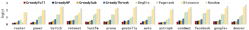
Figure 4: The approximation ratios (lower is better) under random threshold setting. The $y$ axis denotes the approximation ratios of heuristics under the $\log_{10}$ scale. The results are averaged over $10$ initializations of threshold assignments.

Uniform thresholds.

We assign all nodes the same threshold $\tau>3$. We consider different values of the uniform threshold $\tau$ to study how the heuristics perform. Note that as $\tau$ increases, more constant-$0$ nodes emerge in the system because their threshold values are larger than their degrees. Thus, the uniform-threshold setting pushes the performance limits of algorithms by ($1$) setting the thresholds of nodes to be indistinguishable and ($2$) introducing a considerable number of constant-$0$ nodes which makes it harder for the heuristics to even find a feasible solution.

We first present analyses on instances of the same network with different uniform thresholds $\tau$. Due to page limits, we show results for the Google+ network in Fig. 5; the results are similar for all other networks where the Greedy family outperforms the other heuristics in terms of approximation ratios. In particular, the averaged ratios for heuristics in the Greedy family are all less than $3$ for Google+ network, with GreedyThresh having the highest averaged ratio (lower is better) of $2.41$. We also observe when the uniform threshold $\tau$ is large enough, many natural heuristics failed to even find a valid solution due to the presence of a large number of constant-$0$ nodes. This experiment demonstrates the high effectiveness of the proposed framework when nodes have indistinguishable thresholds.

Next, we fix the uniform threshold $\tau$ and analyze the heuristics across all networks. We have investigated different values of $\tau$ from $3$ to $20$, where the Greedy family again outperforms the other heuristics on most instances, producing results that are over 10 times better than baselines. Due to the page limit, we show the results for $\tau=8$ in Fig. 6. Note we omit the results for networks power and peer because they have no feasible solutions when $\tau=8$.

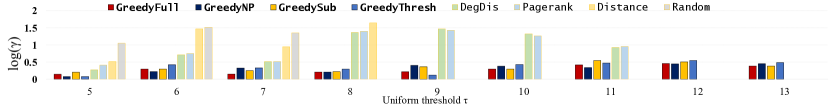
Figure 5: The approximation ratios (lower is better) of heuristics on google+ network under uniform threshold setting. The $y$ axis shows the approximation ratios of heuristics under the $\log_{10}$ scale. Results of several heuristics (DegDis, Pagerank, Distance, Random) are absent for some instances because they failed to find valid fixed points.

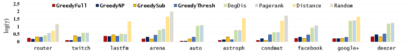
Figure 6: The approximation ratios (lower is better) of heuristics on networks under uniform threshold setting where $\tau=8$. The $y$ axis shows the approximation ratios of heuristics under the $\log_{10}$ scale. Results of several heuristics (DegDis, Pagerank, Distance, Random) are absent for some instances because they failed to find valid fixed points.

Gnp networks.

We study the heuristics on Erdös Rényi networks with sizes up to $1,000$ where thresholds are assigned randomly. We observe that the ratios of GreedyFull/NP/Thresh are all over $40$, and the ratios of GreedySub are as high as $148.48$. We remark that in a gnp network, the state-$1$ nodes in a nontrivial minimum fixed point are often surrounded by nodes with similar thresholds and similar degrees. Our results suggest a limitation of the proposed framework, that is, when networks exhibit uniformity at the node level, the heuristics might not correctly choose state-$1$ nodes to construct a minimum fixed point. Note that such results are expected since NMin-FPE is hard to approximate. We remark that the Greedy family still outperforms baselines on Gnp networks.

Efficiency.

Our results demonstrate that the proposed Greedy NP/Sub/Thresh are more efficient than the ILP solver Gurobi for the tested scenarios. In Table 2, we show the runtime of Greedy NP/Sub/Thresh and Gurobi solver on the two largest networks under the random threshold scenario.

The heuristics achieve high efficiency by the pruning technique. For some networks, Gurobi runs comparably fast, usually within $5$ minutes. Nevertheless, Gurobi uses parallelization mechanisms such as multithreading (over $30$ threads are used on each instance) whereas our heuristics achieve high efficiency while executing in serial mode.

Network	GreedyNP	GreedySub	GreedyThresh	Gurobi
Google+	26.13s	263.64s	32.16s	1153.04s
Deezer	104.76s	395.89s	96.22s	794.89s

Table 2: Execution times of heuristics in seconds.

7 Conclusions and Future Work

In this paper, we study the NMin-FPE problem from both the theoretical and empirical points of view. We establish the computational hardness of the problem and propose effective algorithms for solving NMin-FPE under special cases and general graphs. Our results point to a new way of quantifying system resilience against the diffusion of negative contagions and a new approach to tackle the influence minimization problem. One limitation of the proposed heuristics is the cubic time complexity. Thus, a future direction is to develop more efficient methods for solving NMin-FPE. Another promising direction is to approximate NMin-FPE under restricted graph classes such as regular graphs. Lastly, we want to extend the model to multi-layer networks and investigate problems in this new domain.

References

- [1] Elie M Adam, Munther A Dahleh, and Asuman Ozdaglar. On the behavior of threshold models over finite networks. In 2012 IEEE 51st IEEE Conference on Decision and Control (CDC), pages 2672–2677. IEEE, 2012.
- [2] Simon P Anderson, Jacob K Goeree, and Charles A Holt. Minimum-effort coordination games: Stochastic potential and logit equilibrium. Games and economic behavior, 34(2):177–199, 2001.
- [3] Vincenzo Auletta, Diodato Ferraioli, and Gianluigi Greco. Reasoning about consensus when opinions diffuse through majority dynamics. In IJCAI, pages 49–55, 2018.
- [4] Chris Barrett, Harry B. Hunt III, Madhav V Marathe, S. S. Ravi, Daniel J. Rosenkrantz, Richard E. Stearns, and Mayur Thakur. Predecessor existence problems for finite discrete dynamical systems. Theoretical Computer Science, 386(1):3–37, 2007.
- [5] Christopher L Barrett, Harry B Hunt III, Madhav V Marathe, SS Ravi, Daniel J Rosenkrantz, and Richard E Stearns. Complexity of reachability problems for finite discrete dynamical systems. Journal of Computer and System Sciences, 72(8):1317–1345, 2006.
- [6] Hui Cao, Emre Ertin, and Anish Arora. Minimax equilibrium of networked differential games. ACM Transactions on Autonomous and Adaptive Systems (TAAS), 3(4):1–21, 2008.
- [7] Chen Chen, Hanghang Tong, B Aditya Prakash, Tina Eliassi-Rad, Michalis Faloutsos, and Christos Faloutsos. Eigen-optimization on large graphs by edge manipulation. ACM Transactions on Knowledge Discovery from Data (TKDD), 10(4):1–30, 2016.
- [8] Chen Chen, Hanghang Tong, B Aditya Prakash, Charalampos E Tsourakakis, Tina Eliassi-Rad, Christos Faloutsos, and Duen Horng Chau. Node immunization on large graphs: Theory and algorithms. IEEE Transactions on Knowledge and Data Engineering, 28(1):113–126, 2015.
- [9] Wei Chen, Yajun Wang, and Siyu Yang. Efficient influence maximization in social networks. In Proceedings of the 15th ACM SIGKDD international conference on Knowledge discovery and data mining, pages 199–208, 2009.
- [10] Justin Cheng, Jon Kleinberg, Jure Leskovec, David Liben-Nowell, Karthik Subbian, Lada Adamic, et al. Do diffusion protocols govern cascade growth? In Proceedings of the International AAAI Conference on Web and Social Media, volume 12, 2018.
- [11] Dmitry Chistikov, Grzegorz Lisowski, Mike Paterson, and Paolo Turrini. Convergence of opinion diffusion is pspace-complete. In Proceedings of the AAAI Conference on Artificial Intelligence, volume 34, pages 7103–7110, 2020.
- [12] C. Daskalakis and C. H. Papadimitriou. Computing equilibria in anonymous games. In 48th Annual IEEE FOCS, pages 83–93. IEEE, 2007.
- [13] C. Daskalakis and C. H. Papadimitriou. Approximate Nash equilibria in anonymous games. Journal of Economic Theory, 156:207–245, 2015.
- [14] Ming Dong, Bolong Zheng, Nguyen Quoc Viet Hung, Han Su, and Guohui Li. Multiple rumor source detection with graph convolutional networks. In Proceedings of the 28th ACM International Conference on Information and Knowledge Management, pages 569–578, 2019.
- [15] Eric Goles and Servet Martínez. Neural and automata networks: dynamical behavior and applications, volume 58. Springer Science & Business Media, 2013.
- [16] Mark Granovetter. Threshold models of collective behavior. American journal of sociology, 83(6):1420–1443, 1978.
- [17] M. O. Jackson. Social and economic networks. Princeton university press, Princeton, NJ, 2010.
- [18] David Kempe, Jon Kleinberg, and Éva Tardos. Maximizing the spread of influence through a social network. In Proceedings of the ninth ACM SIGKDD international conference on Knowledge discovery and data mining, pages 137–146, 2003.
- [19] Elias Khalil, Bistra Dilkina, and Le Song. Cuttingedge: influence minimization in networks. In Proceedings of Workshop on Frontiers of Network Analysis: Methods, Models, and Applications at NIPS, pages 1–13. Citeseer, 2013.
- [20] Masahiro Kimura, Kazumi Saito, and Hiroshi Motoda. Minimizing the spread of contamination by blocking links in a network. In Aaai, volume 8, pages 1175–1180, 2008.
- [21] Masahiro Kimura, Kazumi Saito, and Ryohei Nakano. Extracting influential nodes for information diffusion on a social network. In AAAI, volume 7, pages 1371–1376, 2007.
- [22] Chris J. Kuhlman, V. S. Anil Kumar, Madhav V. Marathe, S. S. Ravi, and Daniel J. Rosenkrantz. Inhibiting diffusion of complex contagions in social networks: theoretical and experimental results. Data Min. Knowl. Discov., 29(2):423–465, 2015.
- [23] Chris J. Kuhlman, Gaurav Tuli, Samarth Swarup, Madhav V. Marathe, and S. S. Ravi. Blocking simple and complex contagion by edge removal. In Hui Xiong, George Karypis, Bhavani M. Thuraisingham, Diane J. Cook, and Xindong Wu, editors, 2013 IEEE 13th International Conference on Data Mining, Dallas, TX, USA, December 7-10, 2013, pages 399–408. IEEE Computer Society, 2013.
- [24] Pouria Ramazi, James Riehl, and Ming Cao. Networks of conforming or nonconforming individuals tend to reach satisfactory decisions. Proceedings of the National Academy of Sciences, 113(46):12985–12990, 2016.
- [25] Daniel J Rosenkrantz, Madhav V Marathe, SS Ravi, and Richard E Stearns. Synchronous dynamical systems on directed acyclic graphs (dags): Complexity and algorithms. In Proc. AAAI 2021, pages 11334–113432, 2021.
- [26] Farzad Salehisadaghiani and Lacra Pavel. Distributed nash equilibrium seeking in networked graphical games. Automatica, 87:17–24, 2018.
- [27] Lucas D Valdez, Louis Shekhtman, Cristian E La Rocca, Xin Zhang, Sergey V Buldyrev, Paul A Trunfio, Lidia A Braunstein, and Shlomo Havlin. Cascading failures in complex networks. Journal of Complex Networks, 8(2):cnaa013, 2020.
- [28] Biao Wang, Ge Chen, Luoyi Fu, Li Song, and Xinbing Wang. Drimux: Dynamic rumor influence minimization with user experience in social networks. IEEE Transactions on Knowledge and Data Engineering, 29(10):2168–2181, 2017.
- [29] Don E Willis, Jennifer A Andersen, Keneshia Bryant-Moore, James P Selig, Christopher R Long, Holly C Felix, Geoffrey M Curran, and Pearl A McElfish. Covid-19 vaccine hesitancy: Race/ethnicity, trust, and fear. Clinical and Translational Science, 14(6):2200–2207, 2021.
- [30] Robert M Wolfe and Lisa K Sharp. Anti-vaccinationists past and present. Bmj, 325(7361):430–432, 2002.
- [31] Lan Yang, Zhiwu Li, and Alessandro Giua. Influence minimization in linear threshold networks. Automatica, 100:10–16, 2019.
- [32] Qipeng Yao, Ruisheng Shi, Chuan Zhou, Peng Wang, and Li Guo. Topic-aware social influence minimization. In Proceedings of the 24th International Conference on World Wide Web, pages 139–140, 2015.
- [33] Mengbin Ye, Lorenzo Zino, Žan Mlakar, Jan Willem Bolderdijk, Hans Risselada, Bob M Fennis, and Ming Cao. Collective patterns of social diffusion are shaped by individual inertia and trend-seeking. Nature communications, 12(1):1–12, 2021.
- [34] Sixie Yu, Kai Zhou, Jeffrey Brantingham, and Yevgeniy Vorobeychik. Computing equilibria in binary networked public goods games. In Proceedings of the AAAI Conference on Artificial Intelligence, volume 34, pages 2310–2317, 2020.
- [35] Jianming Zhu, Peikun Ni, and Guoqing Wang. Activity minimization of misinformation influence in online social networks. IEEE Transactions on Computational Social Systems, 7(4):897–906, 2020.