Hybrid CGME and TCGME algorithms for large-scale general-form regularization

Abstract

Two new hybrid algorithms are proposed for large-scale linear discrete ill-posed problems in general-form regularization. They are both based on Krylov subspace inner-outer iterative algorithms. At each iteration, they need to solve a linear least squares problem. It is proved that the inner linear least squares problems, which are solved by LSQR, become better conditioned as $k$ increases, so LSQR converges faster. We also prove how to choose the stopping tolerance for LSQR in order to guarantee that the computed solutions have the same accuracy with the exact best regularized solutions. Numerical experiments are given to show the effectiveness and efficiency of our new hybrid algorithms, and comparisons are made with the existing algorithm.

MSC Classification] 65F22, 65F10, 65J20, 65F35, 65F50

1 Introduction

Consider the large-scale linear discrete ill-posed problem of the form

$$\min_{x\in\mathbb{R}^{n}}\|Ax-b\|\quad{\rm or}\quad Ax=b,\quad A\in\mathbb{R}^{m\times n},\quad b\in\mathbb{R}^{m},$$ (1)

where the norm $\|\cdot\|$ is the 2-norm of a vector or matrix, and $A$ is ill-conditioned with its singular values decaying to zero without a noticeable gap, and the right-hand side $b=b_{true}+e$ is assumed to be contaminated by a Gaussian white noise $e$, where $b_{true}$ is the noise-free right-hand side and $\|e\|<\|b_{true}\|$. Without loss of generality, assume that $Ax_{true}=b_{true}$. Discrete linear ill-posed problems of the form (1) are derived from the discretization of linear ill-posed problems, such as the first kind Fredholm integral equation, and arise in various scientific research and applications areas, including biomedical sciences, geoscience, mining engineering and astronomy; see, e.g., [1, 2, 3, 4, 5, 6, 7, 8, 9, 10, 11, 12, 13].

Because of the presence of the noise $e$ and the high ill-conditioning of $A$, the naive solution $x_{naive}=A^{{\dagger}}b$ to (1) generally is meaningless since it bears no relation to the true solution $x_{true}=A^{{\dagger}}b_{true}$, where ${\dagger}$ denotes the Moore-Penrose inverse of a matrix. To calculate a meaningful solution, it is necessary to employ regularization to overcome the inherent instability of ill-posed problems. The basic idea of regularization is that the underlying problem (1) is replaced with a modified problem which is relatively stable and can obtain a regularized solution to approximate the true solution. There are various regularization techniques taking many forms; see, e.g., [14, 15, 7] for more details.

The simple and popular regularization is the iterative regularization method. In this setting, an iterative method is applied directly to

$$\min_{x\in\mathbb{R}^{n}}\|Ax-b\|$$

and regularization is obtained by terminating early. It is well known that iterative algorithms exhibit semi-convergence on ill-posed problems, with errors decreasing initially but at some point beginning to increase since the small singular values of $A$ start to amplify noise [7, 15, 16]. Therefore, for iterative regularization, the number of iterations plays the role of regularization parameter and a vital and nontrivial task is to select a good stopping iteration which means determining a good regularization parameter. Unfortunately, some iterative algorithms only have partial regularization, which means only an iterative algorithm may not get the best regularized solution; see, e.g., [16, 17, 18] for more details.

The other popular way is the hybrid regularization method. Since O’Leary and Simmons [19] introduce the hybrid method using the Golub-Kahan bidiagonalization process and truncated singular value decomposition (SVD) for large-scale standard-form regularization, various hybrid methods based on the Krylov subspace method have been introduced including more general regularization terms and constraints; see, e.g., [20, 14, 21, 22, 23, 24, 25, 26, 27, 28]. The Hybrid regularization method generally calculates an approximation of $x_{true}$ by solving the following general-form regularization

$$\min_{x\in\mathbb{S}}\|Lx\|\ {\rm subject\ to}\ \mathbb{S}=\left\{x|\|Ax-b\|\leq\tau\|e\|\right\}$$ (2)

or

$$\min_{x\in\mathbb{R}^{n}}\left\{\|Ax-b\|^{2}+\lambda^{2}\|Lx\|^{2}\right\},$$ (3)

where $\tau\approx 1$, $L\in\mathbb{R}^{p\times n}$ is a regularization matrix and usually a discrete approximation of some derivative operators, and $\lambda>0$ is the regularization parameter that controls the amount of regularization to balance the fitting term and the regularization term; see, e.g., [15, 7, 29]. Problem (2) is the discrepancy principle-based general-form regularization which is equivalent to Problem (3) which is the general-form Tikhonov regularization; see [15, pp. 11, 85, 105, 179] and [7, pp.63-4, 172, 181-2] for the equivalence of the above two formulations. The solution to (3) is unique for a given $\lambda>0$ when $N(A)\cap N(L)={0}$ where $N(\cdot)$ denotes the null space of a matrix. When $L=I_{n}$, with $I_{n}$ being the $n\times n$ identity matrix, Problem (2) and Problem (3) are said to be in standard form.

It is worth mentioning that regularization in other norms than the 2-norm is also significant, and some ill-posed problems may have an underlying mathematical model that is not linear. Consider the general optimizations of the form

$$\min_{x\in\mathbb{S}}\mathcal{R}(Lx)\ {\rm subject\ to}\ \mathbb{S}=\left\{x|\mathcal{J}(Ax-b)=\min\right\}$$

or

$$\min_{x\in\mathbb{R}^{n}}\{\mathcal{J}(Ax-b)+\lambda^{2}\mathcal{R}(Lx)\},$$

where $\mathcal{J}$ is a fit-to-data term and $\mathcal{R}$ is a regularization term. It is known, for instance, that solving

$$\min_{x\in\mathbb{S}}\|Lx\|_{p}^{p}\ {\rm subject\ to}\ \mathbb{S}=\{x|\|Ax-b\|_{q}^{q}=\min\}$$ (4)

or

$$\min_{x\in\mathbb{R}^{n}}\{\|Ax-b\|_{q}^{q}+\lambda^{2}\|Lx\|_{p}^{p}\},$$ (5)

where $1\leq q<2$ and $1\leq p<2$. For these cases, one should take advantage of more sophisticated methods to solve nonlinear optimization problems; however, many of these methods require solving a subproblem with an approximate linear model; see, e.g., [20, 23] and [15, pp. 120-121] for more details.

In this paper, we focus our discussion on the linear problem, i.e., Problem (2). The reason we focus our study on Problem (2) instead of Problem (3) is that when we solve (2), the number of iterations plays the regularization parameter, which means that we do not have to determine the optimal regularization parameter prior to the solution at each iteration. The basic idea of the new hybrid method is first to solve the underlying problem (1) by a Krylov solver, and then apply a general-form regularization term to the projected problems which are generated by the Krylov solver. This means that only the constraint of Problem (2) is projected onto a consequence of nested Krylov subspaces and the regularization is retained unchanged. This way, on the one hand, can make full use of the advantages of the Krylov subspace method to reduce the large-scale problem into the small or medium problem. On the other hand, it can also retain as much information as possible. Therefore, what we can expect is that our method can capture the dominant generalized singular value decomposition (GSVD) of the matrix pair $\{A,L\}$ components information as much as possible.

Before proceeding, it should be emphasized that no matter what method is used, the most important basic ingredient for solving (2) and (3) successfully is that the best regularized solution must capture the dominant GSVD components of the matrix pair $\{A,L\}$ and meanwhile suppress those corresponding to small generalized singular values; see, e.g., [15, 7, 30, 31].

Kilmer et al. [30] adapt the joint bidiagonalization (JBD) process proposed by Zha [32] and develop a JBD process that successively reduces the matrix pair $\{A,L\}$ to lower and upper bidiagonal forms, respectively. Based on this process, they propose an iterative algorithm based on projections to solve (3). It is argued [30] that the underlying solution subspaces are legitimate since they appear to be more directly related to the generalized right singular vectors of the pair of matrix $\{A,L\}$ solution subspace. However, in the method, one needs to determine an optimal or suitable regularization parameter for each projected general-form Tikhonov regularization problem, and, in the meantime, one has to judge when the projection subspace is large enough. Unfortunately, the meaning of ‘sufficiently large’ or ‘large enough’ has been vague, and no a deterministic definition has been given without ambiguity up to now. Jia and Yang [31] propose a new JBD process-based iterative algorithm, called the JBDQR algorithm, for solving (2) instead of (3). The JBDQR algorithm using the same JBD process with the one due to Kilmer et al. [30]. Therefore, they have the same underlying solution subspace that is argued to be legitimate. Although they are based on the same JBD process and have the same underlying solution subspace, the mechanism and features of the two algorithms are different and it is argued [31] that JBDQR can be more efficient than the one in [30].

The JBD process is an inner-outer iterative process. At each outer iteration, the JBD process needs to compute the solution of a large-scale linear least squares problem with the coefficient matrix $(A^{T},L^{T})^{T}$ that is larger than the problem itself and supposed to be solved iteratively, called inner iteration. Fortunately, $(A^{T},L^{T})^{T}$ is generally well conditioned, as $L$ is typically so in applications [15, 7]. In these cases, the LSQR algorithm [33] can solve the least squares problems mentioned efficiently. Although the underlying solution subspaces generated by the process are legitimate, the overhead of computation of the methods based on the process may be extremely expensive. Unfortunately, methods based on the JBD process can not avoid solving the large-scale inner least squares problem at every iteration. Finally, methods based on the process need to solve a large-scale least squares problem with the coefficient matrix $(A^{T},L^{T})^{T}$ to form a regularized solution. Therefore, the method based on the JBD process may come at considerable computational costs.

Novati and Russo [34] propose a Arnoldi-Tikhonov (AT) method for solving (3). First, the method uses the Arnoldi process to reduce the underlying matrix $A$ to a sequence of small upper Hessenberg matrix $H_{m}$. Then the regularization matrix $L$ is multiplied by the column orthogonal matrix $W_{m}$, which is generated by the Arnoldi process applied to $A$ with starting vector $b$. In other words, the AT method first projects $A$ onto a sequence of Krylove subspaces, while projects $L$ onto the same Krylov subspaces which have nothing to do with $L$ because they are generated only by $A$ and $b$. Gazzola and Novati [35] propose an iterative algorithm based on the AT method and the discrepancy principle [7, 15] for multiparameter Tikhonov regularization problems. They also present a generalized AT (GAT) method in [24] for solving (3). The difference between the GAT method and the AT method is the parameter selection method. Gazzola and Nagy [23] applying the flexible Krylov subspaces and the restarting Arnoldi algorithm to the AT method obtain two new algorithms for solving (3). Novati and Russo [36] propose an adaptive AT algorithm for image restoration.

These studies about AT and GAT methods are all based on the Arnoldi process. The process requires that the underlying matrix $A$ must be a square matrix, and the process takes advantage of only $A$ but does not use its transpose, so the information on $A^{T}$ is lacking. In fact, for $L=I_{n}$, Hansen [7, p.126] points out that the success of Arnoldi process-based methods is highly problem dependent, because they mix the SVD components in each iteration, and they can be successful when the mixing of the SVD components is weak, e.g., $A$ is (nearly) symmetric. Therefore, these algorithms are not theoretically guaranteed to capture the dominant SVD components of $A$ and because the regularization matrix $L$ is blindly projected to the Krylove subspaces generated only by $A$ and $b$, the algorithms may lose important information on the regularization. Therefore, there is no guarantee that these algorithms can capture the dominant GSVD components of the matrix pair $\{A,L\}$. This may cause the algorithms to fail, or even if the algorithms work, the accuracy of the regularized solution obtained by the algorithms may not be so high, because, as we mentioned above, the key to solving (2) and (3) successfully is that the regularized solution must capture all the needed dominant GSVD components of the matrix pair $\{A,L\}$; see, e.g., [15, 7, 31, 30]. In addition, these algorithms are for solving Problem (3). They need to determine the optimal regularization parameter prior to the solution. In fact, it is hard to prove the optimal regularization parameter of the projected problem is the one of Problem (2).

Gazzola et al. [25] propose an iterative algorithm based on the nonsymmeteric Lanczos process solving (3). First, they review the fundamental Krylov-Tikhonov techniques based on Lanczos bidiagonalization and the Arnoldi algorithms. Then the QMR algorithm based on the nonsymmetric Lancos bidiagonalization process is proposed to solve (3) with $L=I_{n}$ and $L\neq I_{n}$. Finally, they present the theoretical framework based on the Krylov method. Hochstenbach and Reichel [37] propose an iterative method, based on Golub-Kahan bidiagonalization, for solving (3). Viloche Bazn et al. [38] extend the GKB-FP algorithm proposed by Bazán and Borges [28] to general-form Tikhonov regularization. They carry the GKB-FP algorithm over to standard-form transformation and free-of-standard-form transformation, respectively.

All of these studies are based on the Golub-Kahan bidiagonazation process. Just like the AT method and the GAT method, these algorithms, except for the extension of GKB-FP for standard-form transformation, first project the underlying matrix $A$ onto a sequence of Krylov subspaces and then simultaneously project the regularization matrix $L$ onto the same Krylov subspaces. Finally, QR factorization or GSVD and parameter choice methods are used to solve the projected problems. Although Gloub-Kahan process based algorithms, such as LSQR and CGME, has partial or full regularization [18, 16, 17] which means they can capture some or all of the dominant SVD components of $A$, blindly projecting the regularization matrix $L$ onto the Krylov subspaces which only generated by $A$ and $b$, just as we mentioned above, may lost important information about the regularization. As a consequence, these algorithms can not be theoretically guaranteed to capture the dominant GSVD components of $\{A,L\}$, which is crucial to solve (2) and (3) successfully.

In this paper, we propose two new hybrid algorithms for solving (2). First, we exploit a Krylov solver to solve the underlying problem (1). Then a general-form regularization term is applied to the projected problems which are generated by the Krylov solver. Finally, we solve the projected problem with the general-form regularization term. They are inner-outer iterative algorithms. At every iteration, we need to solve a linear least squares problem, called inner iteration. The resulting algorithms are called hybrid CGME and hybrid truncation CGME (TCGME), because the Krylov solvers are the CGME algorithm and the TCGME algorithm presented by Jia in [16], respectively. They are abbreviated as hyb-CGME and hyb-TCGME, respectively.

One of the benefits of our method is that it can capture the dominant SVD components of $A$ and simultaneously it also includes all the information of $L$, therefore, it is can be expected that our method can capture the dominant GSVD of the matrix pair $\{A,L\}$ components information as much as possible, which is the key to solve (2) and (3) successfully. Another benefit is that we no longer determine an optimal regularization parameter for each projected problem with general-form regularization prior to the solution, which itself, unlike the optimal regularization parameter of the original problem (3), may be hard to define because the projected problem may fail to satisfy the discrete Picard condition, so that regularized solutions may behave irregularly. The other benefit is that we avoid solving the large-scale linear least squares problems with the coefficient matrix $(A^{T},L^{T})^{T}$ in JBDQR to obtain the regularized solution, and the size of inner linear least squares problems is much less than the one of JBDQR. Therefore, it is can be expected that our method is substantially cheaper than JBDQR.

We will provide strong theoretical supports for our algorithms by establishing a number of results. we prove that the inner least squares problems to become better conditioned as $k$ increases. Then LSQR chosen to solve the inner least squares problems converges faster as $k$ increases. In principle the inner linear least squares problems are supposed to be solved accurately, but in practice, they are solved by a iterative algorithm since they are large-scale problem. We prove how to choose the stopping tolerance for the iterative algorithm to solve the inner least squares problems, In order to guarantee that the computed regularized solution have the same accuracy as the accurate regularized solution.

The rest of this paper is organized as follows. In Section 2, we briefly review CGME and TCGME. We propose hyb-CGME and hyb-TCGME algorithms and make an analysis on the conditioning of inner least squares problems in Section 3. In Section 4, we make a theoretical analysis on the stopping tolerance for LSQR. Numerical experiments are presented in Section 5. Finally, we conclude the paper in Section 6.

2 The CGME and TCGME algorithms

In this section we provide some necessary background. We describe CGME and TCGME, which are based on the Golub-Kahan bidiagonalization process [39]. Given the initial vectors $\beta_{1}p_{1}=b$ and $\beta_{1}q_{0}=0$, for $i=1,2,3,\cdots$, the Golub-Kahan iterative bidiagonalization computes

$$\alpha_{i}q_{i} = A^{T}p_{i}-\beta_{i}q_{i-1},$$ (6)

$$\beta_{i+1}p_{i+1} = Aq_{i}-\alpha_{i}p_{i},$$ (7)

where $\beta_{i+1}\geq 0$ and $\alpha_{i+1}\geq 0$ are normalization constants chosen so that $\|q_{i}\|=\|p_{i+1}\|=1$. In particular, $\beta_{1}=\|b\|$.

With the definitions

$$Q_{k}=(q_{1},\ldots,q_{k}),\ P_{k}=(p_{1},\ldots,p_{k}),$$ (8)

and

$$B_{k}=\left(\begin{array}[]{cccc}\alpha_{1}&&&\\ \beta_{2}&\alpha_{2}&&\\ &\ddots&\ddots&\\ &&\beta_{k}&\alpha_{k}\\ \end{array}\right)\in\mathbb{R}^{k\times k},\ B_{k+}=\left(\begin{array}[]{c}B_{k}\\ \beta_{k+1}e_{k}^{T}\\ \end{array}\right)\in\mathbb{R}^{{(k+1)}\times k},$$ (9)

where $e_{k}$ is the $k$-th vector of the standard Euclidean basis vector of $\mathbb{R}^{k}$, the recurrence relations (6) and (7) can be written of the form

$$A^{T}P_{k} = Q_{k}B_{k}^{T},$$

$$AQ_{k} = P_{k+1}B_{k+}.$$

These matrices can be computed by the following $k$-step Golub-Kahan bidiagonalization process.

Algorithm 1  $k$-step Golub-Kahan bidiagonalization process.

1:Take $p_{1}=b/\|b\|\in\mathbb{R}^{m}$, and define $\beta_{1}q_{0}=0$.

2:for $\ \textbf{do}j=1,2,\cdots,k$

3:     $r=A^{T}p_{j}-\beta_{j}q_{j-1}$

4:     $\alpha_{j}=\|r\|$;  $q_{j}=r/\alpha_{j}$

5:     $s=Aq_{j}-\alpha_{j}p_{j}$

6:     $\beta_{j+1}=\|s\|$;  $p_{j+1}=s/\beta_{j+1}$.

7:end for

It is well known that CGME [40, 41, 42, 16] is the CG method implicitly applied to

$$\min\|AA^{T}y-b\|\ {\rm or}\ AA^{T}y=b\ {\rm and}\ x=A^{T}y,$$

and it solves the problems

$$\|x_{naive}-x_{k}^{cgme}\|=\min_{x\in\mathcal{V}_{k}}\|x_{naive}-x\|$$

for the iterate $x_{k}^{cgme}$, where $\mathcal{V}_{k}=\mathcal{K}_{k}(A^{T}A,A^{T}b)$ is the $k$ dimensional Krylove subspace generated by the Golub-Kahan bidiagonalization process.

From the $k$-step Golub-Kahan bidiagonalization process, it follows

$${B}_{k}=P_{k}^{T}AQ_{k}.$$ (10)

Noting $\|b\|e_{1}=P_{k}^{T}b$ and (10), we have

$$x_{k}^{cgme}=Q_{k}{B}_{k}^{-1}P_{k}^{T}b.$$ (11)

Therefore, CGME solves a sequence of problems

$$\min\|P_{k}{B}_{k}Q_{k}^{T}x-b\|$$

for $x_{k}^{cgme}$ starting with $k=1$, where the projection $P_{k}{B}_{k}Q_{k}^{T}$, a rank-$k$ approximation to $A$, substitutes $A$ in the underlying ill-posed problem (1).

TCGME [16] solves a sequence of problems

$$\min\|P_{k+1}{C}_{k}Q_{k+1}^{T}x-b\|$$ (12)

for $x_{k}^{tcgme}$ starting with $k=1$, where ${C}_{k}$ is the best rank-$k$ approximation for ${B}_{k+1}$ defined in (9). Obviously, the solution to (12) is

$$x_{k}^{tcgme}=Q_{k+1}{C}_{k}^{-1}P_{k+1}^{T}b.$$ (13)

About the accuracy of the rank-$k$ approximations $P_{k}{B}_{k}Q_{k}^{T}$ and $P_{k+1}{C}_{k}Q_{k+1}^{T}$ to $A$, Jia has established the following results (cf. [16, Theorem 1 and Theorem 5]).

Theorem 1.

For the rank-$k$ approximations $P_{k}{B}_{k}Q_{k}^{T}$ and $P_{k+1}{C}_{k}Q_{k+1}^{T}$ to $A$, $k=1,2,\dots,n-1,$ we have

$$\gamma_{k}^{lsqr}<\gamma_{k}^{cgme}<\gamma_{k-1}^{lsqr},$$ (14)

$$\gamma_{k+1}^{cgme}<\gamma_{k}^{cgme},$$ (15)

$$\gamma_{k}^{tcgme}\leq{\theta}_{k+1}^{k+1}+\gamma_{k+1}^{cgme},$$ (16)

where ${\theta}_{k+1}^{k+1}$ is the smallest singular value of ${B}_{k+}$, $\gamma_{k}^{cgme}=\|A-P_{k}{B}_{k}Q_{k}^{T}\|,\gamma_{k}^{tcgme}=\|A-P_{k+1}{C}_{k}Q_{k+1}^{T}\|,\gamma_{k}^{lsqr}=\|A-P_{k+1}B_{k+}Q_{k}^{T}\|$, and $\gamma_{0}^{lsqr}=\|A\|$.

Jia in [16] points that inequalities (14) imply that $P_{k}{B}_{k}Q_{k}^{T}$ is definitely a less accurate rank-$k$ approximation to $A$ than $P_{k+1}B_{k+}Q_{k}^{T}$ and there is no guarantee that $P_{k}{B}_{k}Q_{k}^{T}$ is a near best rank-$k$ approximation to $A$ even for severely and moderately ill-posed problems. From (15) and (16), it follows that

$$\gamma_{k}^{tcgme}<{\theta}_{k+1}^{k+1}+\gamma_{k}^{cgme}.$$

The above relation implies that when ${\theta}_{k+1}^{k+1}$ is very small, the rank-$k$ approximation $P_{k+1}C_{k}Q^{T}_{k+1}$ to $A$ is more accurate than the rank-$k$ approximation $P_{k}B_{k}Q^{T}_{k}$.

As there is a lack of theory to guarantee that $P_{k}B_{k}Q^{T}_{k}$ and $P_{k+1}C_{k}Q^{T}_{k+1}$ are the best rank-$k$ approximations to $A$, in fact, it is not even theoretically guaranteed that $P_{k}B_{k}Q^{T}_{k}$ and $P_{k+1}C_{k}Q^{T}_{k+1}$ are the near best rank-$k$ approximations to $A$, which means the regularized solution obtained by Krylov solvers, CGME or TCGME, alone possibly only has partial regularization [16]. In other words, the regularized solution obtained by CGME or TCGME alone at semi-convergence point is not the best one. We now recall the semi-convergence phenomenon: at the beginning of the iterative process the iterates converge to $x_{true}$; afterwards the noise $e$ starts to deteriorate the iterates so that they start to diverge from $x_{true}$ and instead converge to $x_{naive}$, which is a well-known basic property of Krylov solvers are used to solve discrete ill-posed problems; see, e.g., [15, 7, 25]. Semi-convergence is due to the fact that the projected problem starts to inherit the ill-conditioning of (1) after a certain number of steps. That is to say, before the best regularized solution is obtained, the projected problems generated by Krylov solvers, CGME and TCGME, start to inherit the ill-condition of (1). In order to get the best regularized solution which is as accurate as the regularized solution with full regularization, we consider to employ the general-form regularization term to the projected problems, which is the basic idea of the hybrid method.

3 New hybrid algorithms

According to the above analysis of the accuracy of the rank-$k$ approximations $P_{k}B_{k}Q_{k}^{T}$ and $P_{k+1}{C}_{k}Q_{k+1}^{T}$ to $A$, we know that CGME and TCGME used to solve (1) only have partial regularization, which illustrates that the iterative regularization which uses CGME or TCGME alone is not sufficient to achieve the best possible regularized solution. In order to obtain the best possible regularized solution, we are interested in a new hybrid method.

We shall propose two projection based hybrid algorithms which solve (2). Our method would be as easy to implement as the JBDQR algorithm and much cheaper than it because at each iteration it solves a inner linear least squares problem, the size of which is significant less than the one of JBDQR, and our method avoids to solve a large-scale linear least squares problem to get the regularized solution; see [31] for more details. We will establish a number of theoretical results and get insight into the effectiveness of the method. Particularly, we will prove how the conditioning of the inner least squares problems changes as $k$ increases and prove how to choose the stopping tolerance of LSQR which is chosen to solve the inner least squares problems.

Now we propose the new hybrid algorithms. First of all, Krylov solvers CGME and TCGME are exploited to solve the underlying problem, respectively, and the $A$ is substituted with the projections $P_{k}{B}_{k}Q_{k}^{T}$ and $P_{k+1}{C}_{k}Q_{k+1}^{T}$ , respectively, which are generated by the Krylov solvers. This means the underlying problem is projected onto

$$\left\|P_{k}{B}_{k}Q_{k}^{T}x-b\right\|=\min\ {\rm or}\ \left\|P_{k+1}{C}_{k}Q_{k+1}^{T}x-b\right\|=\min,\ k=1,2,\cdots,n.$$ (17)

With the iteration, before the semi-convergence point, the projections $P_{k}{B}_{k}Q_{k}^{T}$ and $P_{k+1}{C}_{k}Q_{k+1}^{T}$ are the near best rank-$k$ approximation to $A$, and then becomes ill-conditioned, because the matrices $B_{k}$ and $C_{k}$ have singular values which are rough approximations to the small ones [16, 19]. Next, therefore, we consider to employ a general-form regularization term to the projections in (17), which means we solve the following problem

$$\min_{x\in\mathbb{S}}\|Lx\|\ {\rm subject\ to}\ \mathbb{S}=\left\{x|\left\|P_{k}{B}_{k}Q_{k}^{T}x-b\right\|=\min\right\},\ k=1,2,\cdots,n,$$ (18)

or

$$\min_{x\in\mathbb{S}}\|Lx\|\ {\rm subject\ to}\ \mathbb{S}=\left\{x|\left\|P_{k+1}{C}_{k}Q_{k+1}^{T}x-b\right\|=\min\right\},\ k=1,2,\cdots,n-1.$$ (19)

Problems (18) and (19) can be seen as projecting the constraint of problem (2) onto a consequence of the nested Krylov subspace and retaining the regularization matrix unchanged. The algorithm that solves (2) by computing the solution to (18) is called the hybrid CGME algorithm which is abbreviated as hyb-CGME since the projetions $P_{k}{B}_{k}Q_{k}^{T}$ are generated by CGME. For the same reason, the algorithm that computes the solution to (2) by solving (19) is named the hybrid TCGME algorithm.

If $P_{k}{B}_{k}Q_{k}^{T}$ and $P_{k+1}{C}_{k}Q_{k+1}^{T}$ are the best rank-$k$ approximation to $A$, our new algorithms would be the same as the MTSVD method in [43]. In this sense, the MTSVD method is also a hybrid method, so is the MTRSVD method [44].

With regard to the solution $x_{L,k}^{cgme}$ to (18) and the solution $x_{L,k}^{tcgme}$ to (19), we establish the following results.

Theorem 2.

Let $Q_{k}$ and $Q_{k+1}$ be defined in (8). Then the solution to (18) is

$$x_{L,k}^{cgme}=x_{k}^{cgme}-\left(L(I_{n}-Q_{k}Q_{k}^{T})\right)^{\dagger}Lx_{k}^{cgme},$$ (20)

and the solution to (19) can be written as

$$x_{L,k}^{tcgme}=x_{k}^{tcgme}-\left(L(I_{n}-Q_{k+1}Q_{k+1}^{T})\right)^{\dagger}Lx_{k}^{tcgme},$$ (21)

where $x_{k}^{cgme}$ and $x_{k}^{tcgme}$ are defined in (11) and (13), respectively.

Proof.

Let $P_{cgme}=P_{k}{B}_{k}Q_{k}^{T}$ and $P_{tcgme}=P_{k+1}{C}_{k}Q_{k+1}^{T}$. From Eld$\acute{e}$n [45], we derive at iteration $k$, the solution to (18) is

$$x_{L,k}^{cgme}=(I_{n}-(L(I_{n}-P_{cgme}^{\dagger}P_{cgme}))^{\dagger}L)P_{cgme}^{\dagger}b$$

and to (19) is

$$x_{L,k}^{tcgme}=(I_{n}-(L(I_{n}-P_{tcgme}^{\dagger}P_{tcgme}))^{\dagger}L)P_{tcgme}^{\dagger}b.$$

Combining the above equations with (11) as well as (13), we obtain

$$x_{L,k}^{cgme}=(I_{n}-(L(I_{n}-P_{cgme}^{\dagger}P_{cgme}))^{\dagger}L)x_{k}^{cgme}.$$ (22)

and

$$x_{L,k}^{tcgme}=(I_{n}-(L(I_{n}-P_{tcgme}^{\dagger}P_{tcgme}))^{\dagger}L)x_{k}^{tcgme}.$$ (23)

Since ${B}_{k}$ is invertible and $P_{k}$ and $Q_{k}$ are matrices with orthonormal columns, it is easy to see that

$$P_{cgme}^{\dagger}P_{cgme}=Q_{k}Q_{k}^{T}.$$ (24)

As $C_{k}$ is the best rank-$k$ approximation to $B_{k}$, and $P_{k+1}$ and $Q_{k+1}$ are matrices with orthonormal columns, we have

$$P_{tcgme}^{\dagger}P_{tcgme}=Q_{k+1}Q_{k+1}^{T}.$$ (25)

Throwing (24) into (22) yields (20) and, similarly, bringing (25) into (23) derives (21). ∎

Remark 1.

From the form of the regularized solutions (20) and (21), these two solutions can be thought of as the iterative solutions (11) and (13) derived by CGME and TCGME are modified by $\left(L(I_{n}-Q_{k}Q_{k}^{T})\right)^{\dagger}Lx_{k}^{cgme}$ and $\left(L(I_{n}-Q_{k+1}Q_{k+1}^{T})\right)^{\dagger}Lx_{k}^{tcgme}$, respectively.

Remark 2.

When $L=I_{n}$, recalling (11) and $Q_{k}^{T}Q_{k}=I_{n}$, it follows from (20) that

$$x_{I_{n},k}^{cgme} = x_{k}^{cgme}-\left((I_{n}-Q_{k}Q_{k}^{T})\right)^{\dagger}x_{k}^{cgme}$$

$$= (I_{n}-(I_{n}-Q_{k}Q_{k}^{T}))x_{k}^{cgme}$$

$$= Q_{k}Q_{k}^{T}x_{k}^{cgme}=Q_{k}Q_{k}^{T}Q_{k}{B}_{k}^{-1}P_{k}^{T}b$$

$$= Q_{k}{B}_{k}^{-1}P_{k}^{T}b=x_{k}^{cgme}$$

with $\left((I_{n}-Q_{k}Q_{k}^{T})\right)^{\dagger}=I_{n}-Q_{k}Q_{k}^{T}$ because $(I_{n}-Q_{k}Q_{k}^{T})$ is an orthogonal projection. In the same way, from (13), (21) and $Q_{k+1}^{T}Q_{k+1}=I_{n}$, we derive

$$x_{I_{n},k}^{tcgme} = x_{k+1}^{tcgme}-\left((I_{n}-Q_{k+1}Q_{k+1}^{T})\right)^{\dagger}x_{k}^{tcgme}$$

$$= (I_{n}-(I_{n}-Q_{k+1}Q_{k+1}^{T})x_{k}^{tcgme}$$

$$= x_{k}^{tcgme}.$$

This means that when $L=I_{n}$, the regularized solutions obtained by our hybrid algorithms are the ones to standard-form regularization.

Next, we consider how to calculate the solutions $x_{L,k}^{cgme}$ and $x_{L,k}^{tcgme}$. Obviouly, the first part of them is easy to compute. For the second part, $L(I_{n}-Q_{k}Q_{k}^{T})$ and $L(I_{n}-Q_{k+1}Q_{k+1}^{T})$, it is infeasible or extremely expensive to compute the Moore-Penrose inverses of $L(I_{n}-Q_{k}Q_{k}^{T})$ and $L(I_{n}-Q_{k+1}Q_{k+1}^{T})$ directly, because $L$ is a regularization matrix and large, and therefore these matrix products $L(I_{n}-Q_{k}Q_{k}^{T})$ and $L(I_{n}-Q_{k+1}Q_{k+1}^{T})$ are large and dense.

Let $z_{k}^{cgme}=(L(I_{n}-Q_{k}Q_{k}^{T}))^{\dagger}Lx_{k}^{cgme}$ and $z_{k}^{tcgme}=(L(I_{n}-Q_{k+1}Q_{k+1}^{T}))^{\dagger}Lx_{k}^{tcgme}$. Then $z_{k}^{cgme}$ and $z_{k}^{tcgme}$ are the minimum 2-norm solutions to the least squares problems

$$\min_{z\in\mathbb{R}^{n}}\left\|\left(L(I_{n}-Q_{k}Q_{k}^{T})\right)z-Lx_{k}^{cgme}\right\|$$ (26)

and

$$\min_{z\in\mathbb{R}^{n}}\left\|\left(L(I_{n}-Q_{k+1}Q_{k+1}^{T})\right)z-Lx_{k}^{tcgme}\right\|,$$ (27)

respectively.

Evidently, problems (26) and (27) have the same structures. The only difference between them is $Q_{k+1}$ in (27), which has one more column than $Q_{k}$ in (26). Obviously, they can be solved by the same algorithm. As a consequence, in what follows, we take (26) as an example to study how to solve them.

Due to the large size of $L(I_{n}-Q_{k}Q_{k}^{T})$, we suppose that the problems (26) can only be solved by iterative algorithms. We will use the LSQR algorithm [33] to solve the problem. In order to take fully advantage of the sparsity of $L$ itself and reduce the overhead of computation and the storage memory, it is critical to avoid forming the dense matrix $L(I_{n}-Q_{k}Q_{k}^{T})$ explicitly within LSQR. Note that the only action of $L(I_{n}-Q_{k}Q_{k}^{T})$ in the Lanczos diagonalization process is to form the products of it and its transpose with vectors. We propose Algorithm 2, which efficiently implements the Lanczos bidiagonalization process without forming $L(I_{n}-Q_{k}Q_{k}^{T})$ explicitly.

Algorithm 2 $\widehat{k}$-step Lanczos bidiagonalization process on $L(I_{n}-Q_{k}Q_{k}^{T})$.

1:Taking $\beta_{1}\widehat{u}_{1}=Lx_{k}$, $\beta_{1}=\|Lx_{k}\|$, $w_{1}=L^{T}\widehat{u}_{1}$, and define $\widehat{\beta}_{1}\widehat{v}_{0}=0$.

2:for $\ \textbf{do}j=1,2,\ldots,\widehat{k}$

3:     $\widehat{r}=w_{j}-Q_{k}(Q_{k}^{T}w_{j})-\widehat{\beta}_{j}\widehat{v}_{j-1}$

4:     $\widehat{\alpha}_{j}=\|\widehat{r}\|$;  $\widehat{v}_{j}=\widehat{r}/\widehat{\alpha}_{j}$;  $g_{j}=Q_{k}^{T}\widehat{v}_{j}$

5:     $\widehat{s}=L\widehat{v}_{j}-L(Q_{k}g_{j})-\widehat{\alpha}_{j}\widehat{u}_{j}$

6:     $\widehat{\beta}_{j+1}=\|\widehat{s}\|$;  $\widehat{u}_{j+1}=\widehat{s}/\widehat{\beta}_{j+1}$; $w_{j+1}=L^{T}\widehat{u}_{j+1}$

7:end for

We now consider the solution of (26) using LSQR. Let

$$Q=\left(\begin{array}[]{cc}Q_{k}&Q_{k}^{\perp}\\ \end{array}\right)$$ (28)

be an orthogonal matrix and $Q_{k}^{\perp}\in\mathbb{R}^{n\times(n-k)}$ an orthogonal complement of the matrix $Q_{k}$. With the notation of (28), we have

$$L(I_{n}-Q_{k}Q_{k}^{T})=LQ_{k}^{\perp}(Q_{k}^{\perp})^{T}.$$ (29)

Because $Q_{k}^{\perp}$ is column orthonormal, the nonzero singular values of $LQ_{k}^{\perp}(Q_{k}^{\perp})^{T}$ are identical to the singular values of $LQ_{k}^{\perp}$, we have

$$\kappa(L(I_{n}-Q_{k}Q_{k}^{T}))=\kappa(LQ_{k}^{\perp}(Q_{k}^{\perp})^{T})=\kappa(LQ_{k}^{\perp}).$$ (30)

We now investigate how the conditioning of (26) changes as $k$ increases with the notations.

Theorem 3.

Let the matrix $Q_{k}^{\perp}$ be defined in (28) and $L\in\mathbb{R}^{p\times n}$. When $p\geq n-k$, we obtain

$$\kappa(LQ_{k}^{\perp})\geq\kappa(LQ_{k+1}^{\perp}),\quad k=2,3,\cdots,n-1,$$ (31)

that is,

$$\kappa(L(I_{n}-Q_{k}Q_{k}^{T}))\geq\kappa(L(I_{n}-Q_{k+1}Q_{k+1}^{T})),\quad k=2,3,\cdots,n-1.$$ (32)

Proof.

Exploiting the lemma presenting in [46, pp.78] yields

$$\sigma_{\max}(LQ_{k}^{\perp})\geq\sigma_{\max}(LQ_{k+1}^{\perp}),$$

$$\sigma_{\min}(LQ_{k}^{\perp})\leq\sigma_{\min}(LQ_{k+1}^{\perp}).$$

From the above of the inequalities, we derive

$$\kappa(LQ_{k}^{\perp})=\frac{\sigma_{\max}(LQ_{k}^{\perp})}{\sigma_{\min}(LQ_{k}^{\perp})}\geq\frac{\sigma_{\max}(LQ_{k+1}^{\perp})}{\sigma_{\min}(LQ_{k+1}^{\perp})}=\kappa(LQ_{k+1}^{\perp}),$$

that is, (31) holds. Noticing (29), we directly obtain (32) from (31). ∎

Theorem 3 indicates that, when applied to solve (26), the LSQR algorithm generally converges faster with $k$ because the worst LSQR convergence factor is $\frac{\kappa(LQ_{k}^{\perp})-1}{\kappa(LQ_{k}^{\perp})+1}$, see [47, p. 291]. In particular, in exact arithmetic, LSQR will find the exact solution of (26) after at most $n-k$ iterations.

Exploiting the same method and technology, we can derive similar results for (27), which means that we can use LSQR with Algorithm 2 by replacing $Q_{k}$ with $Q_{k+1}$ to solve (27). This indicates that LSQR with Algorithm 2 computes the Moore-Penrose inverses of $L(I_{n}-Q_{k+1}Q_{k+1}^{T})$ approximately and it is faster convergence as $k$ increases.

Now we present the hyb-CGME and hyb-TCGME algorithms, named Algorithm 3 and Algorithm 4, respectively.

Algorithm 3 (hyb-CGME)  Given $A\in\mathbb{R}^{m\times n}$, $L\in\mathbb{R}^{p\times n}$ and $b\in\mathbb{R}^{n}$, compute the solution $x_{L,k}^{cgme}$.

1:Use Algorithm 1 to compute the projection $P_{k}^{T}B_{k}Q_{k}$.

2:Compute $x_{k}^{cgme}$ by (11).

3:Compute the solution $z_{k}^{cgme}$ to (26) by LSQR with Algorithm 2.

4:Compute the solution $x_{L,k}^{cgme}=x_{k}^{cgme}-z_{k}^{cgme}$ .

Algorithm 4 (hyb-TCGME)  Given $A\in\mathbb{R}^{m\times n}$, $L\in\mathbb{R}^{p\times n}$ and $b\in\mathbb{R}^{n}$, compute the solution $x_{L,k}^{tcgme}$.

1:Use Algorithm 1 to compute the projection $P_{k+1}^{T}{C}_{k}Q_{k+1}$.

2:Compute $x_{k}^{tcgme}$ by (13).

3:Compute the solution $z_{k}^{tcgme}$ to (27) by LSQR with Algorithm 2 replacing $Q_{k}$ with $Q_{k+1}$.

4:Compute the solution $x_{L,k}^{tcgme}=x_{k}^{tcgme}-z_{k}^{tcgme}$ .

We emphasize that, in step 3 of Algorithm 3-4, we will use LSQR with Algorithm 2 to compute the Moore-Penrose inverses approximately in (20) and (21) by solving (26) and (27) with a given tolerance $tol$ as the stopping criterion that substantially exploits the Matlab built-in function lsqr.m without explicitly computing the matrix products $L(I_{n}-Q_{k}Q_{k}^{T})$ and $L(I_{n}-Q_{k+1}Q_{k+1}^{T})$. We will make an insightful analysis in next section and show that the default $tol=10^{-6}$ is generally good enough and larger $tol$ can be allowed in practical applications.

4 The stopping tolerance of LSQR

In this section we establish some important theoretical results on our proposed new algorithms and get insight into how to determine the stopping tolerance of LSQR which is used to solve the inner least squares problems. We only take the hyb-CGME algorithm as an example to analyze the accuracy of the calculated and accurate regularized solution because the hyb-TCGME algorithm is the similar with it. For convenience of writing and without any ambiguity, in what follows, we drop the superscript, which means we will use $z_{k}$, $x_{k}$ and $x_{L,k}$ instead of $z_{k}^{cgme}$, $x_{k}^{cgme}$ and $x_{L,k}^{cgme}$, respectively.

First of all, with the notation in Section 3, we establish the result of the accuracy of the computed solution $\bar{z}_{k}$ with the stopping tolerance $tol$ in the following lemma.

lemma 1.

Let $z_{k}$ and $\bar{z}_{k}$ be the exact solution and the computed solution by LSQR with stopping criterion $tol$ for the problem (26), respectively. Then

$$\frac{\|z_{k}-\bar{z}_{k}\|}{\|z_{k}\|}\leq\frac{\kappa(LQ_{k}^{\perp})}{1-tol\cdot\kappa(LQ_{k}^{\perp})}\left(2+\frac{\kappa(LQ_{k}^{\perp})\|r\|}{\|LQ_{k}^{\perp}\|\|z_{k}\|}\right)tol.$$ (33)

with $r=Lx_{k}-L(I_{n}-Q_{k}Q_{k}^{T})z_{k}$.

Proof.

From [33] it follows that with the stopping tolerance $tol$ the computed solution $\bar{z}_{k}$ is the exact solution to the perturbed problem

$$\min_{z\in\mathbb{R}^{n}}\|(L(I_{n}-Q_{k}Q_{k}^{T})+E_{k})z-Lx_{k}\|,$$ (34)

where

$$E_{k}=-\frac{r_{k}r_{k}^{T}L(I_{n}-Q_{k}Q_{k}^{T})}{\|r_{k}\|^{2}}$$

is the perturbation matrix with $r_{k}=Lx_{k}-L(I_{n}-Q_{k}Q_{k}^{T})\bar{z}_{k}$ and

$$\frac{\|E_{k}\|}{\|L(I_{n}-Q_{k}Q_{k}^{T})\|}=\frac{\|(I_{n}-Q_{k}Q_{k}^{T})L^{T}r_{k}\|}{\|L(I_{n}-Q_{k}Q_{k}^{T})\|\|r_{k}\|}\leq tol.$$

Exploiting the standard perturbation theory [48, p. 382] and (30), we obtain

$$\frac{\|z_{k}-\bar{z}_{k}\|}{\|z_{k}\|}\leq\frac{\kappa(LQ_{k}^{\perp})}{1-tol\cdot\kappa(LQ_{k}^{\perp})}\left(2+(\kappa(LQ_{k}^{\perp})+1)\frac{\|r\|}{\|LQ_{k}^{\perp}\|\|z_{k}\|}\right)tol,$$ (35)

According to the proof of Wedin’s Theorem; see [48, pp. 400], we find that the factor $\kappa(LQ_{k}^{\perp})+1$ in (35) can be replaced by $\kappa(LQ_{k}^{\perp})$ in the context since the right-hand side $Lx_{k}$ in (34) is unperturbed. Therefore, it is easy to get (33) from (35). ∎

In applications, $L$ is typically well conditioned [15, 7], so is $LQ_{k}^{\perp}$ because of the orthonormality of $Q_{k}^{\perp}$. Therefore, the left hand side of (33) is at least as small as ${\cal O}(tol)$ with a generic constant in ${\cal O}(\cdot)$, which means

$$\frac{\|z_{k}-\bar{z}_{k}\|}{\|z_{k}\|}\leq{\cal O}(tol).$$ (36)

Keep in mind that the hyb-CGME solution can be written as $x_{L,k}=x_{k}-z_{k}.$ Define the computed hyb-CGME solution

$$\bar{x}_{L,k}=x_{k}-\bar{z}_{k}.$$

Therefore, we thus derive

$$\|x_{L,k}-\bar{x}_{L,k}\|=\|z_{k}-\bar{z}_{k}\|.$$ (37)

From (36) and (37) it is reasonable to suppose

$$\frac{\|x_{L,k}-\bar{x}_{L,k}\|}{\|x_{L,k}\|}\leq{\cal O}(tol)$$ (38)

since it is generally impossible that $\|x_{L,k}\|$ is much smaller or larger than $\|z_{k}\|$.

Let $x_{L}^{opt}$ be an optimal regularized solution to the problem (2) with the white noise $e$. Then under a certain necessary discrete Picard condition, a GSVD analysis indicates that the error $\|x_{L}^{opt}-x_{true}\|\geq{\cal O}(\|e\|)$ with a generic constant in ${\cal O}(\cdot)$; see [15, p. 83] and [44].

Define $x_{L,k_{0}}$ and $\bar{x}_{L,k_{0}}$ to be the best regularized solution and the computed best regularized solution by hyb-CGME algorithm, respectively. Obviously,

$$\|x_{L,k_{0}}-x_{true}\|\geq\|x_{L}^{opt}-x_{true}\|\geq{\cal O}(\|e\|).$$ (39)

With these notations, the following theorem compares the accuracy of the best regularized solution with the computed best regularized solution.

Theorem 4.

If $L$ is well conditioned and $\|A\|\approx 1$, then

$$\frac{\|x_{L,k_{0}}-x_{true}\|}{\|x_{true}\|}\geq{\cal O}\left(\frac{\|e\|}{\|b_{true}\|}\right).$$ (40)

If

$${\cal O}(tol)<\frac{\|e\|}{\|b_{true}\|},$$ (41)

then

$$\left|\frac{\|\bar{x}_{L,k_{0}}-x_{true}\|}{\|x_{true}\|}-\frac{\|x_{L,k_{0}}-x_{true}\|}{\|x_{true}\|}\right|\leq{\cal O}(tol)$$ (42)

with a generic constant in ${\cal O}(\cdot)$.

Proof.

Supposing that $Ax_{true}=b_{true}$ which means that the noise-free problem of (1) is consistent, we have $\|b_{true}\|\leq\|A\|\|x_{true}\|$. Using the inequality, it follows from (39) that

$$\frac{\|x_{L,k_{0}}-x_{true}\|}{\|x_{true}\|}\approx\|A\|\frac{\|x_{L,k_{0}}-x_{true}\|}{\|b_{true}\|}\geq\|A\|{\cal O}\left(\frac{\|e\|}{\|b_{true}\|}\right).$$

Because by suitable scaling $\|A\|\approx 1$ can always be done, we derive (40) from the above relations. Using (35) and (38) as well as $\|x_{L,k_{0}}\|\approx\|x_{true}\|$ obtains

$$\frac{\|\bar{x}_{L,k_{0}}-x_{true}\|}{\|x_{true}\|} \leq \frac{\|x_{L,k_{0}}-x_{true}\|}{\|x_{true}\|}+\frac{\|x_{L,k_{0}}-\bar{x}_{L,k_{0}}\|}{\|x_{true}\|}$$ (43)

$$= \frac{\|x_{L,k_{0}}-x_{true}\|}{\|x_{true}\|}+\frac{\|x_{L,k_{0}}-\bar{x}_{L,k_{0}}\|}{\|x_{L,k_{0}}\|}\frac{\|x_{L,k_{0}}\|}{\|x_{true}\|}$$

$$\leq \frac{\|x_{L,k_{0}}-x_{true}\|}{\|x_{true}\|}+{\cal O}(tol).$$

On the other hand, we similarly obtain

$$\frac{\|\bar{x}_{L,k_{0}}-x_{true}\|}{\|x_{true}\|}\geq\frac{\|x_{L,k_{0}}-x_{true}\|}{\|x_{true}\|}-{\cal O}(tol).$$ (44)

Combining (43) with (44) obtains

$$\frac{\|x_{L,k_{0}}-x_{true}\|}{\|x_{true}\|}-{\cal O}(tol)\leq\frac{\|\bar{x}_{L,k_{0}}-x_{true}\|}{\|x_{true}\|}\leq\frac{\|x_{L,k_{0}}-x_{true}\|}{\|x_{true}\|}+{\cal O}(tol),$$

which implies (42). ∎

Clearly, (40) and (42) imply that, under condition (41), the computed $\bar{x}_{L,k_{0}}$ is almost the same as the exact $x_{L,k_{0}}$ as an approximation to $x_{true}$. Furthermore, according to the analysis above, we can establish more general results, including Theorem 4 as a special case.

Theorem 5.

If $L$ is well conditioned and $\|A\|\approx 1$, then

$$\frac{\|x_{L,k}-x_{true}\|}{\|x_{true}\|}\geq{\cal O}\left(\frac{\|e\|}{\|b_{true}\|}\right),\ k=1,2,\ldots,\min\{m,n\}.$$ (45)

Let $\bar{x}_{L,k}$ be the computed solutions obtained by Algorithm 3 using LSQR in step 3 with the stopping criterion $tol$. Then if the condition (41) is satisfied, for $k=1,2,\ldots,k_{0}$ and a few $k>k_{0}$ we have

$$\left|\frac{\|\bar{x}_{L,k}-x_{true}\|}{\|x_{true}\|}-\frac{\|x_{L,k}-x_{true}\|}{\|x_{true}\|}\right|\leq{\cal O}(tol)$$ (46)

with a generic constant in ${\cal O}(\cdot)$.

Proof.

Notice that $x_{L,k_{0}}$ is the best possible regularized solutions by hyb-CGME and Algorithm 1 is run for $k=1,2,\ldots,\min\{m,n\}$, i.e.,

$$\frac{\|x_{L,k_{0}}-x_{true}\|}{\|x_{true}\|}=\min_{k=1,2,\ldots,\min\{m,n\}}\frac{\|x_{L,k}-x_{true}\|}{\|x_{true}\|}.$$ (47)

Because the iterates $\|x_{L,k}\|$ exhibits increasing tendency, and it first approximates $x_{true}$ from below for $k=1,2,\cdots,k_{0}$, in later stages, however, the iterates will start to diverge from $x_{true}$. But it will not deviate from $x_{true}$ too much for a few $k>k_{0}$, therefore, for $k=1,2,...,k_{0}\ {\rm and\ a\ few}\ k>k_{0}$, we have

$$\frac{\|x_{L,k}\|}{\|x_{true}\|}={\cal O}(1).$$ (48)

From (47), (48) and the proof of Theorem 4, we attain that when the index $k_{0}$ is replaced by $k=1,2,\ldots,k_{0}$ and a few $k>k_{0}$, (40) and (42) also hold under the condition (41). ∎

Clearly, (45) and (46) imply that, under condition (41), the calculated $\bar{x}_{L,k}$ is almost the same as the exact $x_{L,k}$ as an approximation to $x_{true}$ for $k=1,2,\ldots,k_{0}$ and a few $k>k_{0}$. Although the above analysis is for using LSQR to solve (26), taking advantage of the same method and technique, for solving (27) we can get exactly the same results.

What we have to highlight is that the relative noise level $\frac{\|e\|}{\|b_{true}\|}$ is typically more or less around $10^{-3}$ or $10^{-2}$ in practice applications, three or four orders greater than $10^{-6}$. From the above analysis, we draw the conclusion that it is generally enough to set $tol=10^{-6}$ in LSQR at step 3 of Algorithms 3–4. A smaller $tol$ will result in more inner iterations without any gain in the accuracy of $\bar{x}_{L,k}$ for $k=1,2,\ldots,k_{0}$ and a few $k>k_{0}$. Moreover, Theorems 4–5 indicate that $tol=10^{-6}$ is generally well conservative and larger $tol$ can be used, so that LSQR fewer iterations to achieve the convergence and the hyb-CGME algorithm and the hyb-TCGME algorithm are more efficient.

In summary, the conclusion is that a widely varying choice of $tol$ has no effects on the regularized solution of hyb-CGME and hyb-TCGME, provided that $tol<\frac{\|e\|}{\|b_{true}\|}$ is considerably and the regularization matrix $L$ is well conditioned, but has substantial effects on the efficiency of hyb-CGME and hyb-TCGME.

Finally, we should mention something about the efficiency comparison of Algorithm 3-4 with the JBDQR algorithm which is more efficient than the algorithm in [30]; see [31] for more details. It is obvious that at iteration $k$, Algorithm 3 and 4 cost almost the same computation, since the truncation in Algorithm 4 costs little. And they may be considerably cheaper than JBDQR because JBDQR has to compute a large-scale least squares problem with coefficient matrix $(A^{T},L^{T})^{T}$ which is larger than the problem itself and may be very expensive. Compared with JBDQR, Algorithm 3 and Algorithm 4 only need to solve a large-scale least squares problem with coefficient matrices $L(I_{n}-Q_{k}Q_{k}^{T})$ and $L(I_{n}-Q_{k+1}Q_{k+1}^{T})$, respectively, and it turns out that they become better conditioned with $k$. This means used to solve the inner least squares problems in hyb-CGEM and hyb-TCGME, LSQR converges faster as $k$ increases. The faster LSQR converges, the cheaper our proposed new hybrid algorithms. In addition, to obtain the regularized solution, JBDQR finally has to solve a large-scale linear least squares problem with coefficient matrix $(A^{T},L^{T})^{T}$, which may also be particularly expensive.

5 Numerical experiments

In this section, we report numerical experiments on several problems, including one dimensional and two dimensional problems, to demonstrate that the proposed new hybrid algorithms work well and the regularized solutions obtained by hyb-TCGME are at least as accurate as those obtained by JBDQR, and the proposed new method is considerably more efficient than JBDQR. All the computations are carried out in Matlab R2019a 64-bit on 11th Gen Intel(R) Core(TM) i5-1135G7 2.40GHz processor and 16.0 GB RAM with the machine precision $\epsilon_{\rm mach}=2.22\times 10^{-16}$ under the Miscrosoft Windows 10 64-bit system.

Table 1 lists all test problems together with some of their basic properties, where one dimensional examples from the regularization toolbox [49] and two dimensional problems from the Matlab Image Processing Toolbox and [2, 50]. We denote the relative noise level

$$\varepsilon=\frac{\|e\|}{\|b_{true}\|}.$$

Table 1: The description of test problems.

Problem	Description	Ill-posedness
shaw	one dimensional image restoration model	severe
baart	one dimensional gravity surveying problem	severe
heat	Inverse heat equation	moderate
deriv2	Computation of second derivative	mild
grain	spatially variant Gaussian blur	unknown
mri	symmetric doubly Toeplitz PSF matrix	unknown
satellite	spatially invariant atmospheric turbulence blur	unknown
GaussianBlur440	spatially invariant Gaussian blur	unknown

Let $x^{reg}$ denote the regularized solution obtained by algorithms. We use the relative error

$$\frac{\|L(x^{reg}-x_{true})\|}{\|Lx_{true}\|}$$ (49)

to plot the convergence curve of each algorithm with respect to $k$, which is more instructive and suitable to use the relative error (49) in the general-form regularization context other than the standard relative error of $x_{reg}$; see [15, Theorems 4.5.1-2] and [31] for more details. In the tables to be presented, we will list the smallest relative errors and the total outer iterations required to obtain the smallest relative errors in the braces. We also will list the total CPU time which is counted in seconds by the Matlab built-in commands tic and toc and the corresponding total outer iterations.

For our new algorithms hyb-CGME and hyb-TCGME, we use the Matlab built-in function lsqr with Algorithm 2 avoiding forming the dense matrices $L(I_{n}-Q_{k}Q_{k}^{T})$ and $L(I_{n}-Q_{k+1}Q_{k+1}^{T})$ explicitly to compute (26) and (27) with the default stopping tolerance $tol=10^{-6}$. For the JBDQR algorithm [31], we use the same function with the same stopping tolerance to solve the inner least squares problems, which means the inner least squares problems of JBDQR are solved by the Matlab built-in function lsqr with the same default stopping tolerance $tol=10^{-6}$. We have observed that for each test problem, when taking three $tol=10^{-6},10^{-5}$ and $10^{-4}$, the computed best regularized solutions by hyb-CGME, hyb-TCGME and JBDQR have the same accuracy. As a consequence, if not explicitly stated, we will only report the results on $tol=10^{-6}$.

5.1 One dimension case

For the four test problems we use the code of [49] to generate $A$, the true solution $x_{true}$ and noise-free right-hand side $b_{true}$. They are severely, moderately and mildly ill-posed, respectively. We mention that the test problem deriv2 has three kinds of right-hand sides, distinguished by the parameter ”$example=1,2,3$”. We only report the results on the parameter ”$example=2$” since we have obtained very similar results on the problem with ”$example=1,3$”. In the experiments, we take $m=n=10,000$. Purely for test purposes, we choose $L=L_{1}$ defined by

$$L_{1}=\left(\begin{array}[]{ccccc}1&-1&&&\\ &1&-1&&\\ &&\ddots&\ddots&\\ &&&1&-1\\ \end{array}\right)\in\mathbb{R}^{(n-1)\times n}.$$ (50)

Table 2: The relative errors defined by (33) and the optimal regularization parameters in the braces for the first four test problems in Table 1 with $L=L_{1}$.

	$\varepsilon=10^{-1}$
	hyb-CGME	JBDQR	hyb-TCGME
shaw	0.9908(2)	3.2943(1)	0.2244(7)
baart	0.9663(2)	0.6093(1)	0.5615(4)
heat	0.9516(4)	0.3636(1)	0.3689(13)
deriv2	0.8002(2)	1.2761(1)	0.4805(6)

	$\varepsilon=5\times 10^{-2}$
	hyb-CGME	JBDQR	hyb-TCGME
shaw	0.9770(3)	1.3390(1)	0.2515(7)
baart	0.9869(2)	0.6063(1)	0.5535(3)
heat	0.7805(5)	0.3470(1)	0.3499(15)
deriv2	0.5907(2)	0.9265(1)	0.4443(9)

	$\varepsilon=10^{-2}$
	hyb-CGME	JBDQR	hyb-TCGME
shaw	0.9681(4)	0.3237(1)	0.1972(7)
baart	0.8803(3)	0.7054(1)	0.5500(3)
heat	0.5695(9)	0.2146(5)	0.2128(20)
deriv2	0.6113(2)	0.4359(1)	0.6625(3)

	$\varepsilon=10^{-3}$
	hyb-CGME	JBDQR	hyb-TCGME
shaw	0.3312(6)	0.1246(2)	0.1222(9)
baart	0.5503(3)	0.5257(3)	0.4272(5)
heat	0.3057(15)	0.1427(22)	0.1442(28)
deriv2	0.3826(6)	0.2337(9)	0.5808(2)

From Table 2, we observe that for all four test problems the best regularized solution by hyb-TCGME is at least as accurate as and can be considerably more accurate than that by JBDQR; see, e.g., the results on test problems shaw and baart, and the regularized solution by hyb-CGME is less accurate than that by JBDQR and hyb-TCGME, except for the test problem shaw with $\varepsilon=10^{-1}$ and $\varepsilon=5\times 10^{-2}$ and deriv2 with $\varepsilon=5\times 10^{-3}$. Furthermore, for the test problemsshaw and deriv2, we find the JBDQR algorithm fails while hyb-CGME and hyb-TCGME work very well, especially hyb-TCGME which derives the best regularized solutions with high accuracy with noise levels $\varepsilon=10^{-1}$ and $5\times 10^{-2}$.

Insightfully, we observe from comparing the second column with the fourth column of Table 2 that for each test problem and given $\varepsilon$, hyb-TCGME obtains the best regularized solution that is correspondingly more accurate and requires a correspondingly larger regularization parameter than hyb-CGME. This indicates that, compared with hyb-TCGME, hyb-CGME captures less dominant GSVD components of $\{A,L\}$. Recall the comments at the end of Section 2. CGME only has partial regularization and the rank-$k$ approximation to $A$ obtained by it is less accurate than the counterpart by TCGME. Therefore, the less accurate rank-$k$ approximation to $A$ generated by the projection, the less accurate of the generalized solution obtained by our new hybrid method. This is reasonable, because if the projection capture the less SVD dominant components of $A$, it cannot be expected that the new hybrid method captures all the needed GSVD dominant components of $\{A,L\}$.

By summarizing the above, hyb-TCGME is more effective than hyb-CGME and JBDQR on the test problems. In particular, for severely problems shaw and baart, hyb-TCGME obtained more accurate best regularized solutions.

Table 3: The CPU time of hyb-CGME, JBDQR and hyb-TCGME, the ratio of the CPU time of JBDQR to that of hyb-CGME (times1), the ratio of the CPU time of JBDQR to that of hyb-TCGME (times2), and the total outer iterations (iter) for the first four test problems in Table 1 with $L=L_{1}$.

	$\varepsilon=10^{-1}$
	hyb-CGME	JBDQR	hyb-TCGME	times1	times2	iter
shaw	6.5319	2678.8398	7.4490	410.1164	359.6241	12
baart	3.0381	1940.6978	3.0063	638.7866	645.5436	12
heat	11.9812	2744.7590	8.5197	229.0888	322.1662	20
deriv2	20.1345	8718.1975	26.2901	432.9979	331.6152	20

	$\varepsilon=5\times 10^{-2}$
	hyb-CGME	JBDQR	hyb-TCGME	times1	times2	iter
shaw	7.7211	2652.1893	8.2861	343.4989	320.0769	12
baart	3.7360	1815.0300	3.2283	485.8217	562.2247	12
heat	13.2105	2985.5863	8.6991	226.0010	343.2063	20
deriv2	10.6474	4719.4951	13.7445	443.2533	343.3733	18

	$\varepsilon=10^{-2}$
	hyb-CGME	JBDQR	hyb-TCGME	times1	times2	iter
shaw	8.3601	4120.1932	8.7147	492.8401	472.7865	16
baart	3.1327	1966.6141	3.0570	627.7697	643.3150	12
heat	15.4444	7149.1920	12.5738	462.8987	568.5785	30
deriv2	11.6898	4937.2102	14.9254	422.3520	330.7925	20

	$\varepsilon=10^{-3}$
	hyb-CGME	JBDQR	hyb-TCGME	times1	times2	iter
shaw	8.8225	3440.0999	8.7474	389.9235	393.2711	16
baart	7.5228	7718.6538	7.3403	1026.0346	1051.5447	20
heat	14.2565	8246.0108	11.4969	578.4036	717.2378	40
deriv2	12.5638	4639.1439	14.4195	369.2469	321.7271	20

Recall the analysis of the method based on JBD process of Section 2 and the comments of Section 4. At the same outer iterations, hyb-CGME and hyb-TCGME may be much cheaper than JBDQR, and they may cost the same overhead because the truncation in hyb-TCGME is very cheap. As can be seen from Table 3, for each test problem, the CPU time of hyb-CGME and hyb-TCGME is significantly less than that of JBDQR at the same outer iterations. For the severely ill-posed problems shaw and baart, hyb-CGME and hyb-TCGME take less than ten seconds, respectively, while JBDQR takes almost two thousands of seconds; in particular, for the test problems baart with noise level $\varepsilon=10^{-3}$, our new method only takes no more than 10 seconds, on the other hand, JBDQR takes more than even thousands of seconds. For the moderately and mildly ill-posed problems heat and deriv2, the CPU time of hyb-CGME and hyb-TCGME is less than 20 seconds except for deriv2 with the noise level $\varepsilon=10^{-1}$, the CPU time of hyb-TCGME is 26.2901, a little bit more than 20 seconds. In addition, we also observe from the table that, for each test problem, the new proposed algorithms need almost the same CPU time.

More importantly, we can see from the fifth and sixth columns of the table that the CPU time of JBDQR is almost 300 to 500 times that of hyb-CGME and hyb-TCGME for the test problems shaw and deriv2 with all noise levels. And for the test problem heat with higher noise levels $\varepsilon=10^{-1}$ and $\varepsilon=5\times 10^{-2}$, the CPU time of JBDQR is around 200 to 300 times that of hyb-CGME and hyb-TCGME, however, with lower noise levels $\varepsilon=10^{-2}$ and $\varepsilon=5\times 10^{-3}$, it is even 500 to 700 times. Especially for the severely ill-posed test problem baart, the CPU time of JBDQR is around 400 to 600 times that of hyb-CGME and hyb-TCGME when the noise levels are $10^{-1},5\times 10^{-2}\ {\rm and}\ 10^{-2}$, and the ratio of the CPU time between JBDQR and hyb-CGME and the one between JBDQR and hyb-TCGME are even as high as 1000 when the noise level is $\varepsilon=10^{-3}$. Therefore, hyb-CGME and hyb-TCGME are considerable more efficient than JBDQR on these test problems; in particular, for shaw and baart, hyb-TCGME used much less CPU time and outperformed hyb-CGME and JBDQR very substantially.

Obviously, for these four test problems, hyb-TCGME performs better than JBDQR. Of JBDQR, hyb-TCGME is favorable because of its faster overall convergence and its higher accuracy.

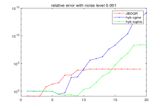
(a)

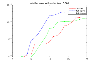
(b)

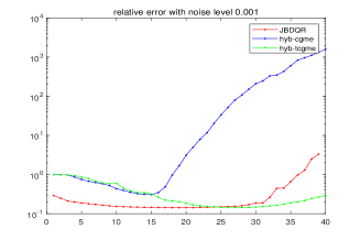
(c)

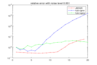
(d)

Figure 1: the relative error of hyb-CGME, JBDQR and hyb-TCGME with $L=L_{1}$ and $\varepsilon=10^{-3}$: (a) baart; (b) shaw; (c) heat; (d) deriv2.

Figure 1 draws the convergence processes of hyb-CGME, JBDQR and hyb-TCGME for $\varepsilon=10^{-3}$. We observe from the figure that the best regularized solutions by hyb-TCGME at semi-convergence point are more accurate than those by hyb-CGME and JBDQR. Moreover, as the figure shows, for every test problem, all three algorithms under consideration exhibit semi-convergence [15, 7]: the convergence curves of the three algorithms first decrease with $k$, then increase. This means the iterates converge to $x_{true}$ in an initial stage; afterwards the iterates start to diverge from $x_{true}$. It is worth mentioning that it is proved [31] that the JBDQR iterates take the form of filtered GSVD expansions, which shows that JBDQR have the semi-convergence property.

In summary, for the four test problems, hyb-TCGME performs best for both accuracy and efficiency, while hyb-CGME is considerably more efficient than JBDQR but a little less accurate than it.

5.2 Two dimension case

In this section, We test the two dimensional image deblurring problems listed in Table 1. The goal in this case is to recover an image $x_{true}$ from a blurred and noisy image $b=b_{true}+e$ .

We consider the problem mri from the Matlab Image Processing Toolbox. The exact image $x_{true}$ of mri is the $15$th slice of the three dimensional MRI image dataset which has $N\times N$ pixels. The blurred operator $A$ is a symmetric doubly Toeplitz PSF matrix and is of Kroneck product form $A=(2\pi\sigma^{2})^{-1}T\otimes T\in\mathbb{R}^{N^{2}\times N^{2}}$, where $T\in\mathbb{R}^{N\times N}$ is a symmetric banded Toeplitz matrix with half-bandwidth $band$ and $\sigma$ controlling the width of Gaussian point spread function (PSF). In what follows, we use $band=16$, $\sigma=2$ and $N=128$. The size of mri is $m=n=128^{2}=16,284$.

For the problems grain, satellite and GaussianBlur440, the size of them is $m=n=2562=65,536$ and they are from [50]. The blurring of the grain is a spatially variant Gaussian blur, satellite is caused by spatially invariant atmospheric turbulence, and GaussianBlur440 is a spatially invariant Gaussian blur. For convenience of writing, satellite and GaussianBlur440 are abbreviated as sate and blur440, respectively.

The regularization matrix is chosen as

$$L=\left(\begin{array}[]{c}I_{N}\otimes L_{1}\\ L_{1}\otimes I_{N}\\ \end{array}\right),$$ (51)

where $L_{1}$ is defined in (50), which is the scaled discrete approximation of the first derivative operator in the two dimensional case incorporating no assumptions on boundary conditions; see [7, Chapter 8.1-2].

Table 4: The relative errors defined by (33) and the optimal regularization parameters in the braces for the latter four test problems in Table 1 with $L$ defined by (51).

	$\varepsilon=10^{-1}$
	hyb-CGME	JBDQR	hyb-TCGME
grain	0.9992(4)	0.9524(9)	0.9601(31)
mri	0.9883(2)	0.9134(6)	0.9169(12)
sate	0.9968(6)	0.9681(13)	0.9682(47)
blur440	0.9913(2)	0.9711(6)	0.9721(21)

	$\varepsilon=10^{5\times-2}$
	hyb-CGME	JBDQR	hyb-TCGME
grain	0.9975(7)	0.9070(19)	0.9237(43)
mri	0.9540(4)	0.8840(12)	0.8873(20)
sate	0.9924(11)	0.9597(26)	0.9597(61)
blur440	0.9855(4)	0.9654(13)	0.9666(39)

	$\varepsilon=10^{-2}$
	hyb-CGME	JBDQR	hyb-TCGME
grain	0.9835(22)	0.7089(71)	0.8005(57)
mri	0.8838(12)	0.8412(51)	0.8448(68)
sate	0.9713(35)	0.9321(132)	0.9345(117)
blur440	0.9717(12)	0.9511(69)	0.9528(159)

	$\varepsilon=10^{-3}$
	hyb-CGME	JBDQR	hyb-TCGME
grain	0.6486(78)	0.5355(225)	0.5727(148)
mri	0.8262(63)	0.7952(461)	0.8003(459)
sate	0.9316(84)	0.9002(377)	0.9077(248)
blur440	0.9514(76)	0.9334(622)	0.9349(895)

Table 4 displays the relative errors and the optimal regularization parameters in the braces of algorithms for the test problems with $\varepsilon=10^{-2},5\times 10^{-2},10^{-2},10^{-3}$ and $L$ defined by (51). We can see that for each test problem the best regularized solution accuracy of JBDQR and hyb-TCGME are very comparable. Importantly, by comparing the results in the second column of Table 4 with those in the fourth column, we observe the same results as in Table 2 that the best regularized solution by hyb-CGME is less accurate than the counterpart by hyb-TCGME. This indicates that if the rank-$k$ approximation to $A$ of the projection is more accurate, the regularized solution is more accurate. This is reasonable just as we mentioned above because a good regularized solution must capture all the needed dominant GSVD components of the matrix pair $\{A,L\}$ and, meanwhile, suppress those corresponding to small generalized singular values; see, e.g.,[15, 7, 30, 31]. The higher the accuracy of the rank-$k$ approximation of the projection to $A$, the more likely it is to ensure that our proposed new algorithms are able to capture all the needed dominant GSVD components of the matrix pair $\{A,L\}$, and the higher the accuracy of the regularized solution obtained by our new method.

Table 5: The CPU time of hyb-CGME, JBDQR and hyb-TCGME, the ratio of the CPU time of JBDQR to that of hyb-CGME(times1), the ratio of the CPU time pf JBDQR to that of hyb-CGME(times2), and the total outer iterations(iter) for the latter four test problems in Table 1 with $L$ defined by (51).

	$\varepsilon=10^{-1}$
	hyb-CGME	JBDQR	hyb-TCGME	times1	times2	iter
grain	33.9623	339.2248	37.3480	9.9883	9.0828	50
mri	7.1192	47.9356	6.9455	6.7333	6.9017	50
satellite	25.4080	230.6816	36.3500	9.0791	6.3461	50
blur440	24.8721	57.2304	42.8874	2.3010	1.3344	50

	$\varepsilon=5\times 10^{-2}$
	hyb-CGME	JBDQR	hyb-TCGME	times1	times2	iter
grain	76.2086	730.3901	72.8844	9.5841	10.0212	100
mri	26.4831	120.9110	26.4821	4.5656	4.5658	100
satellite	62.3031	443.2401	71.8914	7.1143	6.1655	100
blur440	73.8359	112.0466	46.0917	1.5175	2.4309	100

	$\varepsilon=10^{-2}$
	hyb-CGME	JBDQR	hyb-TCGME	times1	times2	iter
grain	365.3413	3094.4985	249.2137	8.4702	12.4170	300
mri	435.0728	1976.4200	422.5347	4.5427	4.6775	500
satellite	281.9240	1764.3952	301.2180	6.2584	5.8575	400
blur440	917.5464	1975.2774	795.1023	2.1528	2.4843	1000

Table 5 reports the results obtained where all the notations and meanings are the same as those in Table 3. As can be seen from the table that for these four test problems with all noise levels, JBDQR takes significantly more CPU time than our new algorithms do, and our new algorithms take almost the same CPU time at the same outer iterations. By observing the results in the fourth and fifth columns of Table 5, we can see that for the test problem grain with all noise levels, the CPU time of JBDQR is almost 10 times that of hyb-CGME and hyb-TCGME. For the test problems mri and satellite, JBDQR takes six to eight times more CPU time than hyb-CGME and hyb-TCGME do, and for the test problem blur440, the CPU time of JBDQR is around two to three times that of hyb-CGME and hyb-TCGME, as shown in Table 5.

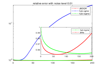
(a)

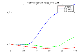
(b)

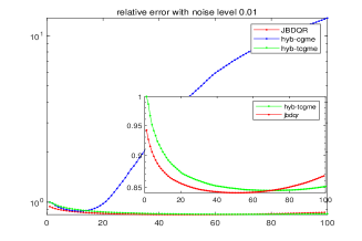
(c)

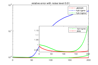
(d)

Figure 2: The relative error of hyb-CGME, JBDQR and hyb-TCGME with $\varepsilon=10^{-2}$ and $L$ defined by (51): (a) blur440; (b) grain; (c) mri; (d) satellite.

In Figure 2 we display the convergence processes of hyb-CGME, JBDQR and hyb-TCGME for $\varepsilon=10^{-3}$ and $L$ defined by (51). We can see that the best regularized solutions by hyb-TCGME are almost same as the counterparts by JBDQR except grain and the best regularized solution by hyb-TCGME and JBDQR is better than that by hyb-CGME for the four test problems. Insightfully, we observe the same phenomenon as Figure 1: for each test problem and every convergence curve initially approaches a regularized solution and then, in later stages of the iterations, converges to some other undesired vector. These results indicate that all three algorithms have the semi-convergence property. We have numerically verified this assertion, and the details are omitted. The semi-convergence property is a desired property because we can exploit the L-curve criterion and the discrepancy principle to estimate the optimal regularized parameter at which the semi-convergence occurs.

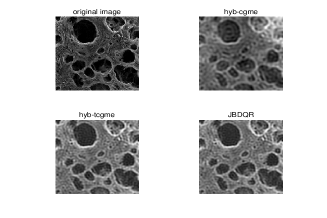
(a)

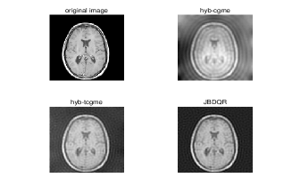
(b)

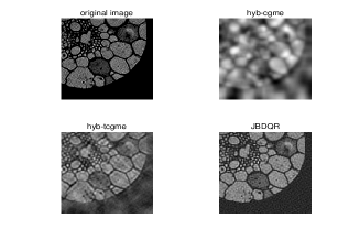
(c)

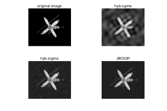
(d)

Figure 3: The exact images and the reconstructed images for the four two dimensional test problems with $\varepsilon=10^{-2}$ and $L$ defined in (51): (a) blur440; (b) mri; (c) grain; (d) satellite.

The exact images and the reconstructed images for the four test problems with $\varepsilon=10^{-2}$ and $L$ defined by (51) are displayed in Figure 3. Clearly, the reconstructed images by hyb-TCGME are at least as sharp as those by JBDQR and the reconstructed images by hyb-TCGME and JBDQR are much more sharp than the counterparts by hyb-CGME .

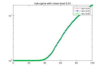
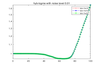
Figure 4: The convergence process of grain with $\varepsilon=10^{-2}$ and $L$ defined by (51).

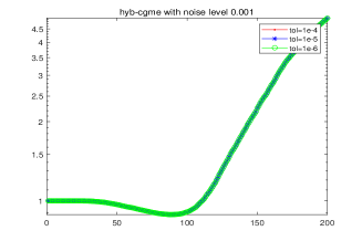
(c)

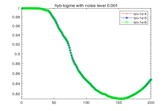
(d)

Figure 5: The convergence process of grain with $\varepsilon=10^{-3}$ and $L$ defined by (51).

In the end, taking the test problem grain as an example, in Figures 4 and 5, we draw the convergence processes of it with $\varepsilon=10^{-2}$ and $\varepsilon=10^{-3}$, respectively, where different stopping tolerances of LSQR are used to solve the inner least squares problems. Clearly, we find that hyb-CGME and hyb-TCGME behave very similarly. We can observe that the convergence curves are indistinguishable in Figures 4–5 when taking three stopping tolerances $tol=10^{-6},10^{-5}\ {\rm and}\ 10^{-4}$. Actually, for each test problem in Table 1, we have observed the same results. These results confirm Theorems 4-5.

6 Concluding remarks and future work

we have proposed two new hybrid algorithms hyb-CGME and hyb-TCGME for solving (3). The number of iterations plays the regularized parameter in our new hybrid algorithms, so it does not have to determine the optimal regularized parameter prior to the solution at every iteration. Therefore it is easy to implement our algorithm.

We have established a number of theoretical results on hyb-CGME and hyb-TCGME and made a detailed analysis on them. We have proved that the conditioning of inner least squares problems becomes better conditioned as the regularization parameter $k$ increases. As a result, LSQR generally converges faster with $k$ and uses fewer iterations. In the meantime, we have made a detailed analysis on the stopping tolerance of LSQR for solving inner least squares problems and shown how to choose it to guarantee that the computed regularized solutions have the same accuracy as the accurate regularized solutions. Numerical experiments have confirmed our theorems.

Numerical experiments have shown that our hyb-TCGME algorithm can compute regularized solutions with very comparable accuracy to the JBDQR algorithm, and hyb-TGCME is significantly more efficient than JBDQR. It turns out hyb-TCGME should at least be a highly competitive alternative of JBDQR. On the other hand, numerical experiments also demonstrate that although our hyb-CGME algorithm is not as accurate as JBDQR, it is considerably more efficient than JBDQR.

There are some important problems that deserve future considerations. The GCV and WGCV methods are $\|e\|$-free parameter choice methods which can be used when the noise level or the estimation of the noise level is unknown in advance. However, the GCV or WGCV parameter-choice method is not directly applicable to our hyb-CGME and hyb-TCGME algorithm, and some nontrivial effects are needed to derive the corresponding GCV or WGCV function. We will consider the GCV and WGCV parameter-choice method for hyb-CGME and hyb-TCGME in future work.

Declarations

We would like to declare that the general content of the manuscript, in whole or in part, is not submitted, accepted, or published elsewhere, including conference proceedings, while it is under consideration or in production.

This work was funded by department of Zhejiang Educational Committee (No. Y202250116).

References

- \bibcommenthead
- Aster et al. [2018] Aster, R.C., Borchers, B., Thurber, C.H.: Parameter Estimation and Inverse Problems. Elsevier, New York (2018)
- Berisha and Nagy [2012] Berisha, S., Nagy, J.: Restore tools: Iterative methods for image restoration (2012). http://www.mathcs.emory.edu/∼nagy/RestoreTools
- Engl [1992] Engl, H.W.: Regularization Methods for the Stable Solution of Inverse Problems, Univ., Institut für Mathematik (1992)
- Engl et al. [1996] Engl, H.W., Hanke, M., Neubauer, A.: Regularization of Inverse Problems vol. 375. Springer Science & Business Media (1996)
- Epstein [2007] Epstein, C.L.: Introduction to the Mathematics of Medical Imaging. SIAM, Philadelphia, PA (2007)
- Haber [2014] Haber, E.: Computational Methods in Geophysical Electromagnetics. SIAM, Philadelphia, PA (2014)
- Hansen [2010] Hansen, P.C.: Discrete Inverse Problems: Insight and Algorithms. SIAM, Philadelphia, PA (2010)
- Kaipio and Somersalo [2006] Kaipio, J., Somersalo, E.: Statistical and Computational Inverse Problems vol. 160. Springer Science & Business Media (2006)
- Kern [2016] Kern, M.: Numerical Methods for Inverse Problems, John Wiley & Sons (2016)
- Kirsch et al. [2011] Kirsch, A., et al.: An Introduction to the Mathematical Theory of Inverse Problems vol. 120. Springer, New York (2011)
- Miller [1970] Miller, K.: Least squares methods for ill-posed problems with a prescribed bound. SIAM J. Math. Anal. 1(1), 52–74 (1970)
- Natterer [2001] Natterer, F.: The Mathematics of Computerized Tomography, SIAM (2001)
- Vogel [2002] Vogel, C.R.: Computational Methods for Inverse Problems, SIAM (2002)
- Chung and Gazzola [2021] Chung, J., Gazzola, S.: Computational methods for large-scale inverse problems: A survey on hybrid projection methods. arXiv preprint arXiv:2105.07221 (2021)
- Hansen [1998] Hansen, P.C.: Rank-deficient and Discrete Ill-posed Problems: Numerical Aspects of Linear Inversion. SIAM, Philadelphia, PA (1998)
- Jia [2020a] Jia, Z.: Regularization properties of krylov iterative solvers cgme and lsmr for linear discrete ill-posed problems with an application to truncated randomized svds. Numer. Algor. 85(4), 1281–1310 (2020)
- Jia [2020b] Jia, Z.: The low rank approximations and ritz values in lsqr for linear discrete ill-posed problem. Inverse Problems 36(4), 045013 (2020)
- Jia [2020c] Jia, Z.: Regularization properties of lsqr for linear discrete ill-posed problems in the multiple singular value case and best, near best and general low rank approximations. Inverse Problems 36(8), 085009 (2020)
- O’Leary and Simmons [1981] O’Leary, D.P., Simmons, J.A.: A bidiagonalization-regularization procedure for large scale discretizations of ill-posed problems. SIAM J. Sci. Stat. Comput. 2(4), 474–489 (1981)
- Chung and Gazzola [2019] Chung, J., Gazzola, S.: Flexible krylov methods for regularization. SIAM J. Sci. Comput. 41(5), 149–171 (2019)
- Chung and Palmer [2015] Chung, J., Palmer, K.: A hybrid lsmr algorithm for large-scale tikhonov regularization. SIAM J. Sci. Comput. 37(5), 562–580 (2015)
- Chung and Saibaba [2017] Chung, J., Saibaba, A.K.: Generalized hybrid iterative methods for large-scale bayesian inverse problems. SIAM J. Sci. Comput. 39(5), 24–46 (2017)
- Gazzola and Nagy [2014] Gazzola, S., Nagy, J.G.: Generalized arnoldi–tikhonov method for sparse reconstruction. SIAM J. Sci. Comput. 36(2), 225–247 (2014)
- Gazzola and Novati [2014] Gazzola, S., Novati, P.: Automatic parameter setting for arnoldi–tikhonov methods. J. Comput. Appl. Math. 256, 180–195 (2014)
- Gazzola et al. [2015] Gazzola, S., Novati, P., Russo, M.R.: On krylov projection methods and tikhonov regularization. Electron. Trans. Numer. Anal. 44(1), 83–123 (2015)
- Gazzola and Sabaté Landman [2019] Gazzola, S., Sabaté Landman, M.: Flexible gmres for total variation regularization. BIT Numer. Math. 59(3), 721–746 (2019)
- Lampe et al. [2012] Lampe, J., Reichel, L., Voss, H.: Large-scale tikhonov regularization via reduction by orthogonal projection. Linear Algebra Appl. 436(8), 2845–2865 (2012)
- Viloche Bazan et al. [2014] Viloche Bazan, F.S., Cunha, M.C., Borges, L.S.: Extension of gkb-fp algorithm to large-scale general-form tikhonov regularization. Numer. Linear Algebra with Appl. 21(3), 316–339 (2014)
- Tihonov [1963] Tihonov, A.N.: Solution of incorrectly formulated problems and the regularization method. Soviet Math. 4, 1035–1038 (1963)
- Kilmer et al. [2007] Kilmer, M.E., Hansen, P.C., Espanol, M.I.: A projection-based approach to general-form tikhonov regularization. SIAM J. Sci. Comput. 29(1), 315–330 (2007)
- Jia and Yang [2020] Jia, Z., Yang, Y.: A joint bidiagonalization based iterative algorithm for large scale general-form tikhonov regularization. Appl. Numer. Math. 157, 159–177 (2020)
- Zha [1996] Zha, H.: Computing the generalized singular values/vectors of large sparse or structured matrix pairs. Numerische Mathematik 72(3), 391–417 (1996)
- Paige and Saunders [1982] Paige, C.C., Saunders, M.A.: Lsqr: An algorithm for sparse linear equations and sparse least squares. ACM Trans. Math. Software 8(1), 43–71 (1982)
- Novati and Russo [2014] Novati, P., Russo, M.R.: A gcv based arnoldi-tikhonov regularization method. BIT Numerical mathematics 54, 501–521 (2014)
- Gazzola et al. [2013] Gazzola, S., Novati, P., et al.: Multi-parameter arnoldi-tikhonov methods. Electron. Trans. Numer. Anal 40, 452–475 (2013)
- Novati and Russo [2014] Novati, P., Russo, M.R.: Adaptive arnoldi-tikhonov regularization for image restoration. Numerical Algorithms 65, 745–757 (2014)
- Hochstenbach and Reichel [2010] Hochstenbach, M.E., Reichel, L.: An iterative method for tikhonov regularization with a general linear regularization operator. The Journal of Integral Equations and Applications, 465–482 (2010)
- Viloche Bazan et al. [2014] Viloche Bazan, F.S., Cunha, M.C., Borges, L.S.: Extension of gkb-fp algorithm to large-scale general-form tikhonov regularization. Numerical Linear Algebra with Applications 21(3), 316–339 (2014)
- Golub and Kahan [1965] Golub, G., Kahan, W.: Calculating the singular values and pseudo-inverse of a matrix. J. Soc. Indust. Appl. Math. Ser. B Numer. Anal. 2(2), 205–224 (1965)
- Björck [2015] Björck, Å.: Numerical Methods in Matrix Computations vol. 59. Springer, Texts in Applied Mathematics (2015)
- Hanke [2001] Hanke, M.: On lanczos based methods for the regularization of discrete ill-posed problems. BIT Numer. Math. 41(5), 1008–1018 (2001)
- Hnětynková et al. [2009] Hnětynková, I., Plešinger, M., Strakoš, Z.: The regularizing effect of the golub-kahan iterative bidiagonalization and revealing the noise level in the data. BIT Numer. Math. 49(4), 669–696 (2009)
- Hansen et al. [1992] Hansen, P.C., Sekii, T., Shibahashi, H.: The modified truncated svd method for regularization in general form. SIAM J. Sci. Comput. 13(5), 1142–1150 (1992)
- Jia and Yang [2018] Jia, Z., Yang, Y.: Modified truncated randomized singular value decomposition (mtrsvd) algorithms for large scale discrete ill-posed problems with general-form regularization. Inverse Probl. 34(5), 055013 (2018)
- Eldén [1982] Eldén, L.: A weighted pseudoinverse, generalized singular values, and constrained least squares problems. BIT Numer. Math. 22(4), 487–502 (1982)
- Golub and Van Loan [2013] Golub, G.H., Van Loan, C.F.: Matrix Computations. Johns Hopkins University Press, Baltimore (2013)
- Björck [1996] Björck, Å.: Numerical Methods for Least Squares Problems. SIAM, Philadelphia, PA (1996)
- Higham [2002] Higham, N.J.: Accuracy and Stability of Numerical Algorithms. SIAM, Philadelphia, PA (2002)
- Hansen [2007] Hansen, P.C.: Regularization tools version 4.0 for matlab 7.3. Numer. Algor. 46(2), 189–194 (2007)
- Nagy et al. [2004] Nagy, J.G., Palmer, K., Perrone, L.: Iterative methods for image deblurring: a matlab object-oriented approach. Numer. Algor. 36(1), 73–93 (2004)