Benchmarking Robustness in Neural Radiance Fields

Abstract

Neural Radiance Field (NeRF) has demonstrated excellent quality in novel view synthesis, thanks to its ability to model 3D object geometries in a concise formulation. However, current approaches to NeRF-based models rely on clean images with accurate camera calibration, which can be difficult to obtain in the real world, where data is often subject to corruption and distortion. In this work, we provide the first comprehensive analysis of the robustness of NeRF-based novel view synthesis algorithms in the presence of different types of corruptions.

We find that NeRF-based models are significantly degraded in the presence of corruption, and are more sensitive to a different set of corruptions than image recognition models. Furthermore, we analyze the robustness of the feature encoder in generalizable methods, which synthesize images using neural features extracted via convolutional neural networks or transformers, and find that it only contributes marginally to robustness. Finally, we reveal that standard data augmentation techniques, which can significantly improve the robustness of recognition models, do not help the robustness of NeRF-based models. We hope that our findings will attract more researchers to study the robustness of NeRF-based approaches and help to improve their performance in the real world.

1 Introduction

Novel View Synthesis (NVS), a long-standing problem in computer vision and computer graphics research, aims to generate photo-realistic images at unseen viewpoints of a 3D scene given a set of posed images. Existing works, including those of image-based rendering, primarily rely on explicit geometry and hand-crafted heuristics [10, 36, 51], which require sophisticated design, extensive efforts for data collection and preprocessing and have difficulty in generalizing to new scenes and settings.

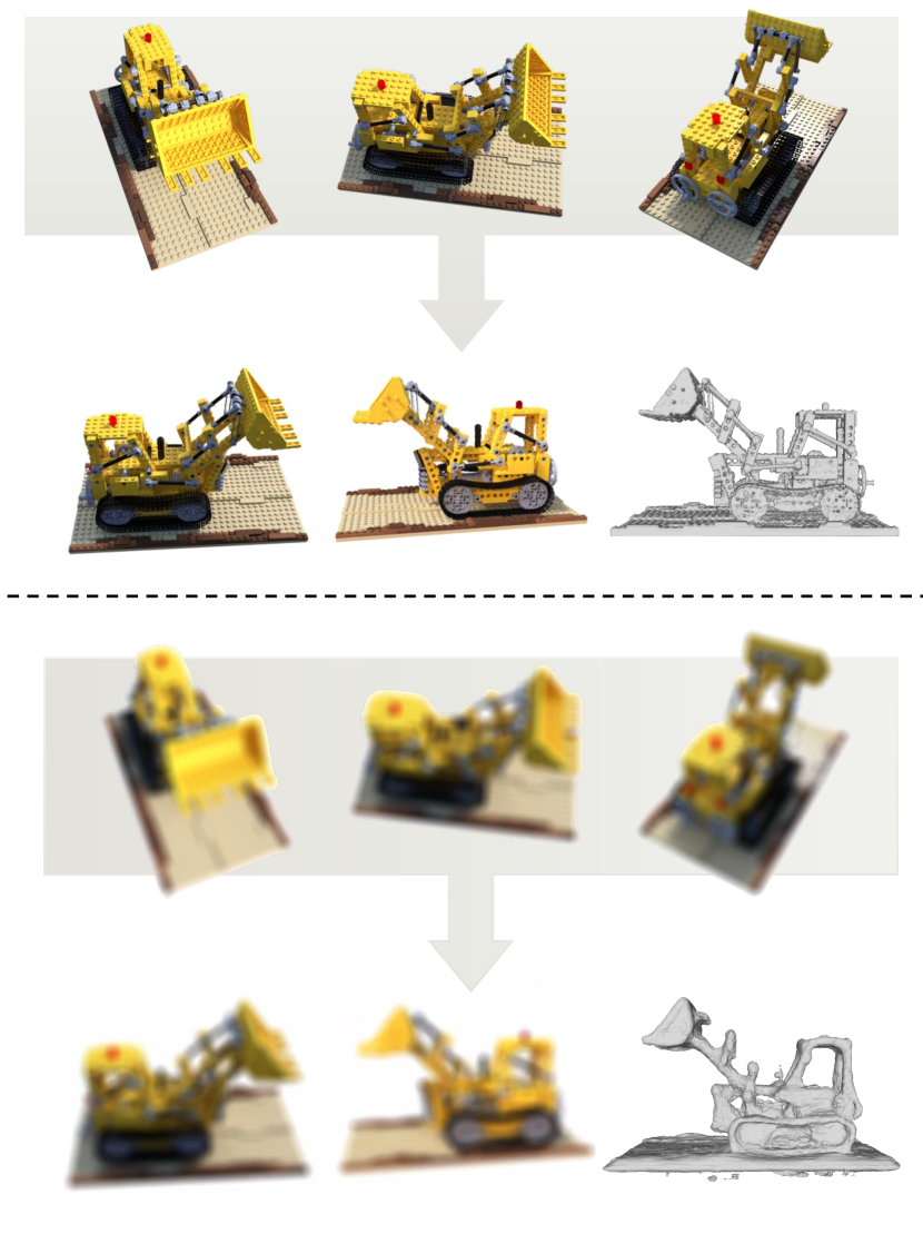
Figure 1: NeRF produces high quality novel view synthesis and accurate surface reconstruction when training on clean images (top). However, corruption on training images will significantly affect both the renderings and geometry of the objects (bottom). Meshes were obtained with marching cubes [19].

Recently, Neural Radiance Fields (NeRF) [24] have demonstrated as an effective implicit 3D scene representation over recent years and achieved state-of-the-art performance on NVS by leveraging end-to-end learnable components with 3D geometry context to reconstruct input images. NeRF encodes a scene into a continuous multi-layer perceptron (MLP), which regresses color and density given any 3D location and view direction. Novel views can thus be synthesized through differentiable volumetric rendering from arbitrary viewpoints.

The emergence of NeRF has made NVS more usable in real-world scenarios by reducing the need for tedious preprocessing steps. In practice, we only have to take images with our phones and estimate camera poses with off-the-shelf structure-from-motion (SfM) techniques to train NeRF-based approaches, which can achieve remarkable view synthesis results with accurately calibrated poses and clean images. However, to generate photo-realistic images at novel viewpoints, it is necessary to comprehensively model the 3D space, including the scene geometry, illumination, and reflections. This requires capturing local high-frequency details, which can make NeRF-based methods sensitive and fragile to perturbations in the inputs. In addition, NeRF-based methods are often optimized using a pixel-based L2 reconstruction loss, which can lead to overfitting the target scene without prior information. When the inputs are corrupted, such as being compressed in JPEG format or blurred due to motion, the reconstructed scenes may exhibit visible artifacts. Most importantly, corruptions often occur during the real-world capture and preprocessing stages. It may seem evident that they can lead to inaccurate reconstruction, but the more important and interesting question—how different types and severities of corruption affect the robustness of NeRF—remains open.

As a step forward, in this paper, we present the first benchmark to comprehensively evaluate the robustness of current NeRF-based methods. Firstly, we construct two benchmarking datasets: LLFF-C and Blender-C, both of which are the corrupted counterparts of the standard datasets used in NeRF-based methods, and the latter also contains 3D-aware corruptions. Using the metrics we propose, we show that modern NeRF-based models exhibit significant degradation across all types of corruptions, and that there is still a significant opportunity for improvement on both LLFF-C and Blender-C. In addition, difficulties for each corruption type exhibit a totally different nature in NeRF-based methods from recognition tasks. Especially, for generalizable methods that use image features to assist neural rendering, we find that scaling the feature encoder does not enhance robustness. We also show that fine-tuning a pretrained generalizable model leads the model to overfit the “incorrect” data, sometimes resulting in worse synthesis quality than using the pretrained model directly.

In summary, the contributions of our paper include:

• We present the first framework for benchmarking and assessing the robustness of NeRF-based systems to visual corruptions.

• Our findings demonstrate that current NeRF-based methods perform poorly under corruptions, including those generalizable ones.

• We systematically analyze and discuss the robustness of NeRF-based methods under various corruptions, feature encoder design, etc.

• We find that standard image data-augmentation techniques do not improve the robustness of novel view synthesis that relies on cross-view consistency.

2 Related Work

Novel view synthesis with NeRF. Traditional image-based rendering methods generate novel views by warping and blending input frames [8, 18], and learning-based methods predict blending weights through neural networks or hand-crafted heuristics [9, 31, 30]. Different from these, geometry-based methods render images through an explicit 3D model, e.g., Thies et al.  [36] stored neural textures on 3D meshes and rendering with standard graphics pipeline. Other 3D proxies such as point clouds [32, 1], voxel grids [27, 16], multi-plane images [23, 34, 51] are also used. However, these approaches often require large amounts of data and memory to produce satisfying results.

Recently, neural fields [45] leverages an MLP to represent 3D shapes or scenes by encoding them into signed-distance, occupancy, or density fields. Among them, NeRF [24] demonstrated remarkable results for novel view synthesis with posed images. NeRF uses a coordinate-based MLP representation and obtains color by differentiable volumetric rendering. The optimization of NeRF can be simply done by minimizing the photometric loss at training camera viewpoints. Although NeRF has been investigated in several aspects, e.g., generation [25], 3D recontruction [43, 40], 3D super-resolution [38], in this work, we still focus on the novel view synthesis task.

Robustness benchmarks. The robustness of deep learning models is crucial for real-world applications, and its assessment has received growing attention in recent years [12, 28, 17]. ImageNet-C [12] benchmark, as one of the pioneering works, evaluates image classifiers’ robustness under simulated image corruptions such as motion blur and jpeg compression. Imagenet-V2 [28] creates new test sets for ImageNet and CIFAR-10 and evaluates the accuracy gap caused by natural distribution shift. Specifically for object recognition, ObjectNet [2] presents a real-world test set containing objects with random backgrounds, rotations, and imaging viewpoints. ImageNet-A [14] and ImageNet-R [11] further propose additional benchmarks for natural adversarial examples and abstract visual renditions like image style, camera operation, and geographic location etc.

Researchers have also examined benchmarks beyond image classification. RobustNav [4] quantifies the performance of embodied navigation agents when exposed to both visual and dynamic corruptions. Ren et al.  [29] provide a taxonomy of common 3D corruptions and identify the atomic corruptions for point clouds for the first time, followed by an evaluation of existing point cloud classification models. More recently, Kar [17] proposes 3D common corruptions that resemble real-world ones by integrating geometry information i.e., depth, into the corruption process. However, a comprehensive benchmark for evaluating the robustness of NeRF is still lacking.

Improving model robustness. Adversarial training [21] is a common method used to protect models from corruption. For example, Xie et al.  [44] show that adversarial perturbations can be used as data augmentation and improve image classification accuracy. Similar conclusions are also reached in natural language processing [39].

On the other hand, data augmentation can significantly improve generalization performance, and many works augment input images to boost recognition. Mixup [49] enforces neural networks to favor linear behavior between training examples by creating convex interpolated samples. Similarly, CutMix [48] also mixes two images, but embeds one in a part of another. Augmix [13] creates compositions of multiple augmented samples that preserve original semantics and statistics. However, mixup [49] and cutmix [48] are not suitable for NeRF augmentation as they disturb the cross-view constraint required by NeRF, while the efficacy of augmix [13] remains to be studied.

To increase the robustness of NeRF, Aug-NeRF [6] firstly proposes a triple-level augmentation training pipeline that is robust to noisy inputs. Some works tackle specific corruptions, e.g., Deblur-NeRF [20] for blurred images, NAN-NeRF [26] for burst noise. Our work differs from them in that we aim to evaluate the robustness of standard NeRF methods and seek ways to improve them.

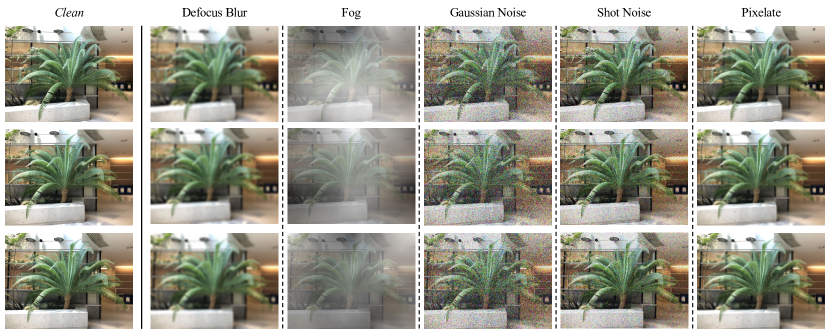
Figure 2: Examples of our proposed LLFF-C on the fern scene under five corruption types at the severity of 2.

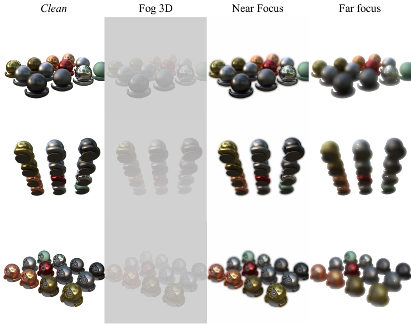
Figure 3: Examples of our proposed Blender-C (left) on the materials scene under 3D-aware corruptions, from which we can see that the same corruption has varying effects across scene depth.

3 Background

We present a benchmark for evaluating the robustness of rendering models that utilize NeRF [24]. This section provides an overview of NeRF and our classification of NeRF-based methods.

3.1 NeRF for Novel View Synthesis

NeRF represents a 3D scene as a continuous function, which takes as inputs a 5D vector containing 3D position $\mathbf{x}=(x,y,z)$ and viewing direction $\mathbf{d}=(\bm{\theta},\bm{\phi})$, and outputs the corresponding radiance $\mathbf{c}(\mathbf{x},\mathbf{d})=(r,g,b)$ with volume density $\sigma(\mathbf{x})$. NeRF is typically parameterized as an MLP $f:(\mathbf{x},\mathbf{d})\rightarrow(\mathbf{c},\sigma)$.

NeRF is an emission-only model, i.e., the color of a pixel only depends on the radiance along the viewing ray. Therefore, according to volume rendering [15], the color along the camera ray $\mathbf{r}(t)=\mathbf{o}+t\mathbf{d}$ that shots from the camera center $\mathbf{o}$ in direction $\mathbf{d}$ can be calculated via standard volume rendering, the discrete format is expressed as the following:

$$F\hat{\mathbf{C}}(\mathbf{r})=\sum_{i=1}^{N}T_{i}(1-\mathrm{exp}(-\sigma_{i}\delta_{i}))c_{i},$$ (1)

$$T_{i}=\mathrm{exp}(-\sum_{j=1}^{i-1}\sigma_{j}\delta_{j}),$$ (2)

where $N$ is the number of sampled points along the ray, $\delta_{i}=t_{i+1}-t_{i}$ is the distance between two adjacent samples, $c_{i}$ and $\sigma_{i}$ are the per-point radiance and density, and $T_{i}$ denotes the accumulated transmittance.

NeRF is trained to minimize the mean-squared error (MSE) between the predicted renderings and the corresponding ground-truth color:

$$\mathcal{L}_{\mathrm{MSE}}=\frac{1}{|\mathcal{R}|}\sum_{r\in\mathcal{R}}\|\hat{\mathbf{C}}(\mathbf{r})-\mathbf{C}(\mathbf{r})\|^{2},$$ (3)

where $\mathcal{R}$ denotes the batch of rays randomly sampled from all training images or one specific image. $\hat{\mathbf{C}}(r)$ and $\mathbf{C}(r)$ are the ground truth and output color of ray $r$. This per-pixel optimization lacks holistic spatial understanding and might make NeRF sensitive to disturbance in pixel values.

After the emergence of NeRF, several other methods based on NeRF have been proposed for novel view synthesis. Although they differ in many aspects, e.g., sampling strategy, positional encoding, network architecture etc, all of them aggregate colors and densities of discontinuous points along viewing rays via differentiable volumetric rendering to synthesize novel views, which are named NeRF-based methods. Non-NeRF-based neural rendering methods obtain pixel colors using explicit representations [32, 37], e.g., point clouds or surface-based implicit representation [46] without volume densities.

3.2 Two genres of NeRF-based methods

We further divide NeRF-based methods into two categories: scene-specific and generalizable. Scene-specific methods such as [24, 3] optimize a single model from scratch with a set of training images of one scene, leading to different network parameters for each scene. In contrast, generalizable methods [41, 5, 47] firstly train a model on a dataset containing hundreds of 3D scenes, then directly infer or fine-tune a few steps on a single testing scene. Specifically, generalizable methods contain CNN or transformer encoders $\bm{F}$ to extract image features from inputs $\mathcal{I}_{i},i=1,2,...n$:

$$\bm{f}_{i}=\bm{F}({\mathcal{I}_{i}}),$$ (4)

For a 3D point $\bm{p}$, image features $\bm{f}_{i}$ across input views are aggregated by the function $\mathcal{A}$. $\mathcal{A}$ is quite different in different methods, but often it consists of a series of operations: perspective projection $\bm{p}$ into input each image, image feature interpolation, and multi-view feature fusion (e.g., cost volume, pooling or simple concatenation):

$$\bm{f}_{\bm{p}}=\mathcal{A}(\bm{f}_{i};\bm{p}),$$ (5)

The features are further decoded to the color $\mathbf{c}_{\bm{p}}$ and density $\sigma_{\bm{p}}$ of $\bm{p}$:

$$\mathbf{c}_{\bm{p}} =\mathcal{D}_{c}(\bm{f}_{\bm{p}};\bm{z}_{c}),$$ (6)

$$\sigma_{\bm{p}} =\mathcal{D}_{\sigma}(\bm{f}_{\bm{p}};\bm{z}_{\sigma}),$$ (7)

where $\bm{z}_{c}$ and $\bm{z}_{\sigma}$ are optional auxiliary vectors (e.g., visibility) to enhance decoding, $\mathcal{D}_{c}$ and $\mathcal{D}_{\sigma}$ denote the decoding networks (mostly MLPs) for color and density respectively ($\mathcal{D}_{c}$ and $\mathcal{D}_{\sigma}$ sometimes share the parameters). With colors and densities for queried 3D points, the final pixel color can be similarly obtained using Equation (1).

4 Corruptions and Test Suite

In this section, we present a detailed description of the structure of our benchmark. Our study focuses on the impact of corruption on NeRF-based models, and we primarily conduct experiments on NeRF-based novel view synthesis methods. However, our test suite can also be directly applied to recent non-NeRF-based methods, such as the one presented in [35], as described in Section 5.1. Additionally, the test suite can be easily adapted to other tasks that involve NeRF, e.g., relighting, reconstruction, and video synthesis.

The goal of our work is to act as a foundation for building robust NeRF-based systems in the real world. Unlike previous benchmarks [12], each data chunk in ours is not a single image, but a 3D scene comprising multi-view images of one scene. Scene-specific methods are optimized directly on “corrupted” unseen scenes, while generalizable methods have already been pretrained on clean training scenes and then tested or finetuned on corrupted target scenes. To avoid confusion, in this paper, training set only refers to the 3D scenes used for pretraining generalizable methods, while target training set and target testing set refer to the training and testing images for a specific target scene or object. The corruptions are drawn from a predefined set which we will elaborate in the following.

4.1 Corruptions

Similar to images, scene corruptions are artifacts that degrade the quality of a system’s RGB observations. The corruptions we include have the following characteristics: (1) the target training set and target testing set have the same lighting conditions; and (2) corrupted images and their clean counterparts are taken from the same camera poses, with only the content altered. We provide around ten types (the exact number depends on the dataset) of corruptions e.g., gaussian noise and fog, mainly from those proposed in [12] and exclude those that do not meet the above requirements. Each corruption has three levels of severity ($1\xrightarrow{}3$) indicating an increase in the degree of degradation.

4.2 Datasets

LLFF-C. LLFF [23] consists of 8 real-world scenes that contain mainly forward-facing images. Each of the eight images is held out as the target testing set. We corrupt the target training set in each scene with 9 corruptions to create the LLFF-C test suite (see Figure 2 for an example).

Blender-C. Blender-C is constructed based on the Blender dataset (also known as NeRF-Synthetic) [22] that contains 8 detailed synthetic objects with 100 images taken from virtual cameras arranged on a hemisphere pointed inward. Inspired by [17], we specifically create 3D-aware fog, near focus, and far focus on replacing their 2D counterparts for Blender-C (see Figure 3). For example, in 3D-aware fog, pixels far from the camera are occluded to a higher extent. The RGB images and the corresponding depth maps are rendered with the official blend files for 3D-aware corruptions. We use 100 images as the target training set and 25 images as the target testing set for each scene.

4.3 Task and Metrics

The task of our benchmark is novel view synthesis learned from images of a 3D scene. The standard procedure for evaluating the performance of novel view synthesis methods is to compare the ground truth images and predicted images at testing viewpoints with the three mostly used metrics: Peak Signal-to-Noise Ratio (PSNR) and Structural Similarity Index Measure (SSIM) [42] and LPIPS [50]. For scene-specific models, we directly provide a corrupted target training set for each model. Generalizable methods are trained on clean training scenes but perform inference or finetuning on corrupted target scenes.

Inspired by the 2D common corruptions on images [12] and point clouds [29], the first step for evaluation is to optimize (inference or finetune for generalizable methods) a model $f$ with a set of clean images and compute the relevant metrics $m_{\mathrm{clean}}^{f},m\in M$ at the target testing set. Next, the same process will be repeated, but with corrupted target training set for each corruption type $c$ and severity $s$. We then calculated the metrics again, which are denoted by $m_{\mathrm{c,s}}^{f},m\in M$. Thus, the corruptions metric (CM) is defined as the mean metric over severities:

$$\mathrm{CM}_{c,m}=\frac{1}{3}\sum_{s=1}^{3}m_{c,s},$$ (8)

Different from classification benchmarks, we do not use another baseline model as the denominator in Equation (8) because it washes out the models’ absolute performance on the corrupted data. Mean CM is thus the average of CM over all the corruption types:

$$\mathrm{mCM}_{m}=\frac{1}{N}\sum_{c}\mathrm{CM}_{c,m},$$ (9)

where $N$ is the number of corruption types.

While $\mathrm{CM}$ and $\mathrm{mCM}$ measure the absolute robustness of NeRF-based models, we are also interested in their relative performance drop, i.e., the amount a model degrades from clean inputs to corrupted ones, defined by Relative mCM as the following:

$$\mathrm{RCM}_{c,m}=\frac{1}{3}\sum_{s=1}^{3}\frac{|m_{\mathrm{clean}}-m_{c,s}|}{m_{\mathrm{clean}}},$$ (10)

$$\mathrm{RmCM}_{m}=\frac{1}{N}\sum_{c}\mathrm{RCM}_{c,m},$$ (11)

where $m\in M$. We use absolute $|m_{\mathrm{clean}}-m_{c,s}|$ in $\mathrm{RCM}_{c,m}$ considering that PSNR and SSIM are higher the better, while LPIPS is lower the better.

5 Experiment

5.1 Setup

We benchmark a total of seven methods, all of which are representative of recent novel view synthesis works. For scene-specific methods, we include NeRF [24], MipNeRF [3], and the network-free method Plenoxels [7]. For generalizable methods, we experiment with IBRNet [41] and MVSNeRF [5]. We also include Generalizable Patch-Based Neural Rendering (GPNR) [35], the latest pure transformer-based architecture, as we were interested in its robustness compared to other methods. We omit PixelNeRF [47] due to its poor performance on datasets other than its testing set, DTU.

For all of the methods, we use publicly available codebases and checkpoints, re-training some as necessary. For IBRNet [41] and MVSNeRF [5], we present results for both direct inference and fine-tuning. The details of dataset processing, training, etc., for each method are included in the supplementary material.

		Noise			Blur			Weather	Digital
	Clean	Gauss.	Shot	Impulse	Defocus	Glass	Motion	Fog	Pixel	JPEG
NeRF	27.68/0.151	24.32/0.297	23.74/0.300	24.04/0.297	20.84/0.501	22.26/0.372	19.20/0.483	11.87/0.528	24.28/0.302	25.29/0.288
MipNeRF	27.69/0.159	23.96/0.340	23.34/0.345	23.69/0.341	20.86/0.510	22.24/0.380	19.10/0.507	12.03/0.545	24.22/0.316	22.13/0.257
Plenoxel	27.45/0.100	20.72/0.480	20.31/0.486	17.71/0.494	20.45/0.509	21.91/0.373	19.20/0.463	12.44/0.660	23.81/0.289	24.78/0.300
MVSNeRF	17.03/0.409	16.78/0.545	16.50/0.551	16.72/0.550	17.13/0.576	17.33/0.500	16.30/0.558	12.97/0.567	17.65/0.448	17.37/0.465
MVSNeRF (ft)	23.94/0.244	21.51/0.442	21.17/0.443	21.41/0.441	20.58/0.517	21.62/0.408	19.42/0.490	13.12/0.606	22.70/0.353	23.15/0.349
IBRNet	25.71/0.158	21.88/0.452	21.36/0.455	22.05/0.434	20.54/0.514	21.77/0.392	19.39/0.453	13.74/0.453	23.35/0.311	23.91/0.338
IBRNet (ft)	27.80/0.112	24.03/0.321	21.33/0.451	23.83/0.322	19.67/0.517	21.84/0.395	19.45/0.456	13.33/0.501	22.82/0.341	24.67/0.311
GPNR	24.58/0.210	21.56/0.481	21.11/0.482	21.43/0.476	20.31/0.530	21.38/0.418	19.13/0.483	12.83/0.569	22.82/0.341	23.34/0.346

Table 1: PSNR$\uparrow$ / LPIPS$\downarrow$ results for clean and corrupted data on LLFF-C, ft indicates results after fine-tuning for generalizable methods.

		Noise			Blur				Weather	Digital
	Clean	Gauss.	Shot	Impulse	Near Focus	Far Focus	Glass	Motion	Fog	Pixel	JPEG
NeRF	30.98/0.071	22.02/0.163	19.21/0.208	23.75/0.167	26.99/0.127	24.81/0.158	22.48/0.210	20.73/0.233	15.44/0.200	26.81/0.138	28.34/0.117
MipNeRF	33.34/0.061	22.68/0.149	19.59/0.211	24.94/0.178	27.92/0.099	25.93/0.121	22.49/0.208	21.04/0.211	15.52/0.184	27.66/0.118	29.74/0.098
Plenoxel	32.94/0.035	20.53/0.556	17.68/0.603	22.41/0.461	27.68/0.100	25.73/0.116	22.28/0.210	21.10/0.225	15.62/0.477	26.56/0.130	28.58/0.115
MVSNeRF	19.56/0.288	15.68/0.559	14.26/0.603	15.36/0.599	19.17/0.310	18.98/0.322	18.24/0.357	17.21/0.364	14.11/0.467	19.28/0.316	19.26/0.314
MVSNeRF (ft)	23.28/0.199	17.72/0.512	16.12/0.561	18.25/0.538	18.25/0.538	22.87/0.217	22.58/0.208	21.38/0.255	14.33/0.406	22.87/0.220	23.03/0.217
IBRNet	27.15/0.143	20.45/0.489	18.16/0.535	21.49/0.499	24.98/0.142	23.80/0.212	21.74/0.270	20.64/0.254	15.28/0.237	24.87/0.120	25.64/0.120
IBRNet (ft)	29.91/0.081	20.97/0.483	19.97/0.496	22.36/0.489	24.88/0.126	22.72/0.197	21.42/0.203	19.95/0.210	15.17/0.256	23.94/0.177	23.81/0.186

Table 2: PSNR$\uparrow$ / LPIPS$\downarrow$ results for clean and corrupted data on Blender-C, ft indicates results after fine-tuning for generalizable methods.

5.2 Results and Findings

We report the $\mathrm{CM}$ values of PSNR and LPIPS on LLFF-C and Blender-C at Table 7 and Table 8. Figure 4 shows part of the qualitative results. Other results, including $\mathrm{CM}$ values of SSIM and detailed $\mathrm{RmCM}$ can be found in the supplementary materials.

Generally, all state-of-the-art methods suffer a performance drop from the clean setting across all corruptions. As seen in Figure 5, methods that achieve better quality on clean data mostly excel in $\mathrm{mCM}$, with scene-specific models more robust than generalizable ones. However, it seems that the corruption robustness is mainly explained by the model’s original ability for scene representation since, by looking at $\mathrm{RmCE}$, no models have demonstrated a remarkable ability to resist corruption.

In terms of relative robustness, Plenoxel [7] and IBRNet (ft) [41] have the highest $\mathrm{RmCM}$ on LLFF-C ($25.5\%/331\%$ and $25.7\%/271\%$ for PSNR/LPIPS) and Blender-C ($31.7\%/751\%$ and $28.1\%/248\%$ for PSNR/LPIPS). Moreover, as a voxel-based approach, Plenoxel [7] sometimes consumes much higher GPU memory on corrupted data than usual due to incorrect density distributions in the empty space of optimized 3D scenes. Also, from Figure 4, we can find it struggles with Gaussian Noise and Fog. This reveals that explicit representation might not be suitable for highly corrupted situations. MVSNeRF [5] has the lowest $\mathrm{RmCM}$ on both datasets because its $m_{\mathrm{clean}}$ is fairly low and leaves little room for degradation. Generalizable methods without finetuning are more relatively robust, maybe due to their prior knowledge learned from massive training data.

Not all corruptions are equally severe. For example, Pixelate and JPEG Compression only lead to an absolute drop of PSNR in less than 15%. However, Fog is the hardest of all methods, resulting in a nearly 50% absolute drop in PSNR for all methods except MVSNeRF [5]. The main reason for this huge discrepancy is that the Pixelate and JPEG have limited influence on original inputs, while Fog corruption leads to a drastic change in images, i.e., occludes the objects with fog (see Figure 2). The difficulties of recognition tasks and 3D reconstruction can also vary. From [12], for image classification, Fog is the easiest corruption type, while Glass Blur is the hardest.

With regard to generalizable methods, fine-tuning on clean data significantly boosts models’ performance (See the first column in Table 7 and Table 8). However, this does not hold for corrupted data. Although MVSNeRF [5] improves on all corruptions because of its generalization performance, IBRNet [41] drops on both datasets across several corruptions, with the largest degradation occurring at severity levels $>1$. The main reason is that highly corrupted scenes disrupt the multi-view consistency that NeRF training relies on, and fine-tuning on such data causes the pretrained network to overfit incorrect geometries. An example can be found in Figure 4.

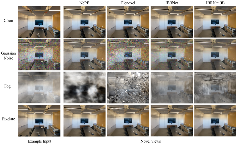
Figure 4: Qualitative results across corruptions (severity = 3) and methods on the room scene. Note we hereby use multiple input images for the scene and only show one example. We can see that each method behaves differently under these corruptions. We encourage the readers to zoom in for a better inspection.

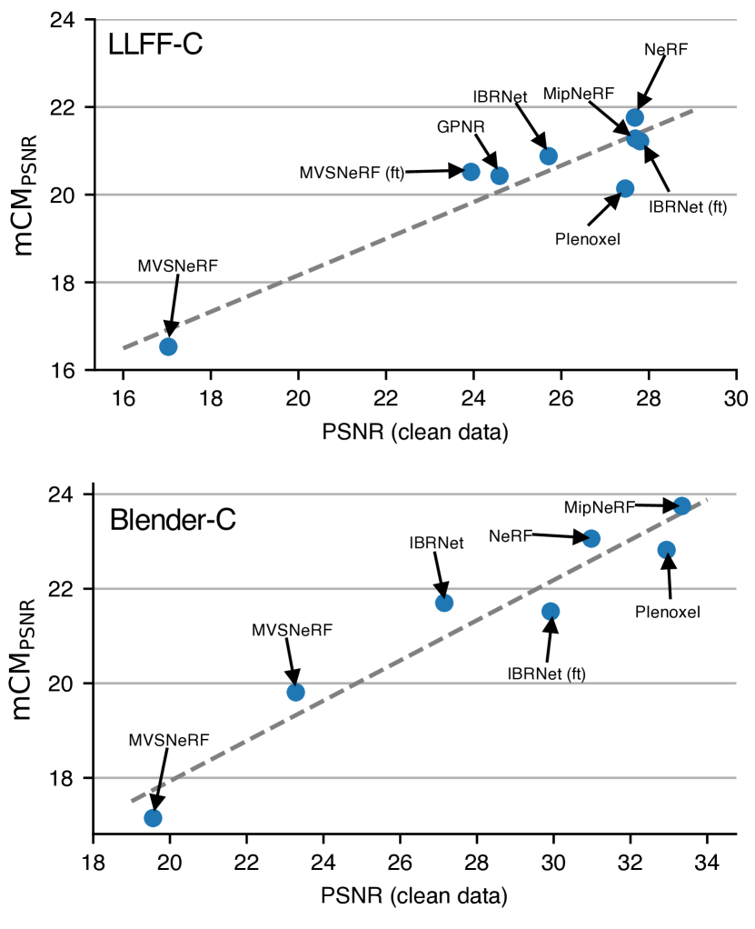
Figure 5: Robustness (mCM) of PSNR values on LLFF-C and Blender-C.

6 Discussion

In this section, we discuss various design and training details in NeRF-based systems and explore how they affect model robustness.

Feature encoding. As mentioned in Section 3.2, generalizable methods include an encoder $\bm{F}$ for image feature extraction. However, different existing methods have different encoder designs. For example, IBRNet [41] uses a U-Net structure containing several downsampling residual blocks and upsampling layers, resulting in 7.96 GFlops and 8.92M parameters, while MVSNeRF [5] only has a few convolutional downsampling layers with 484.5 MFlops and 42.26k parameters. It is important to understand whether the choice of the encoder impacts both the quality of novel view synthesis and the robustness of generalizable methods. The number of parameters also has a direct impact on total training time, as volume rendering is already quite time-intensive.

Therefore, we present additional control studies on IBRNet [41] and MVSNeRF [5] with encoders of different design choices by decreasing the channels of IBRNet’s encoder or residual blocks (Please found the architecture details in the supplementary). We re-trained both methods on the IBRNet Collected and LLFF released scenes. Since the direct inference performance of MVSNeRF [5] remains poor, we continue fine-tuning each target testing scene. The results are reported on Table 3.

		IBRNet			MVSNeRF (ft)
Encoder	Flops	PSNR	SSIM	LPIPS	PSNR	SSIM	LPIPS
ResUNet	7.96G	20.82	0.593	0.421	20.55	0.702	0.453
ResNet	2.62G	20.97	0.593	0.422	20.53	0.701	0.454
ResUNet-Small	2.22G	20.81	0.593	0.422	20.50	0.700	0.456
ResUNet-Tiny	1.09G	20.84	0.594	0.420	20.52	0.700	0.454
MVSNeRF	0.48G	20.76	0.586	0.424	20.58	0.702	0.453

Table 3: Robustness results with different encoder designs.

According to the results, surprisingly, the choices of encoder contribute marginally both to clean data and corruption data. However, training time does vary, e.g., in IBRNet, the total time for training ResUNet-Tiny compared with ResUNet-Big is reduced by more than 60%. This suggests that only low-level features are needed for generalizable models in current frameworks, and the results might be more related to the feature aggregation part.

Patch-based sampling. Recall that NeRF-based methods randomly sample a batch of rays in each training iteration and compare their predicted color with ground truth, which ensures ray diversity while training. Here, we explore another patch-based sampling strategy in which we sample $m$ numbers of $n\times n$ image patches instead, and $m\times n\times n$ equals the number of rays per iteration. We experiment with $n=2,4$ on NeRF [22] and MVSNeRF [5], and find that it drops performance on clean data, but improves the absolute robustness on Fog ($0.1$ and $0.2$ PSNR increase respectively). With $n=2$, they are also more relatively robust.

Data augmentation. We study if data-augmentation techniques help to improve NeRF-based methods’ resistance to visual corruption. We sought image data augmentation at generalizable methods originally designed for classification to help the encoders extract more robust features. However, most augmentations disturb the pixel values and even corrupt the semantic information, making it impossible to train with NeRF-based methods. We test on Augmix [13] that offer minimal deviation on the original image. We augment each image of a training scene with the same set of hyperparameters and train IBRNet [41], MVSNeRF [5] and GPNR [35], and fail to observe improvements upon these methods, for example, IBRNet trained with augmentation have a 0.35 and 0.13 drop in PSNR for clean and corrupted inputs. The main reason those image-based data augmentation offers limited help is that the augmented scenes fail to correspond to a real physical 3D scene, so NeRF-based methods cannot find enough cross-view information to be trained with. We also removed the random crop and random flip operation originally in IBRNet, and found a performance drop in both clean and corrupted data (PSNR decreases by 0.17 and 0.15, respectively).

Pose estimation. In the real-world scenario, structure-from-motion algorithms would be applied to estimate camera poses for each input image. It often fails with sparse or textureless inputs, let alone corrupted images that are difficult to find enough correspondence. Therefore, as part of our study, we also study how image corruption would influence bundle adjustment. We tested the commonly used open-source COLMAP framework [33] on the real-world dataset LLFF-C. During the experiment, we found that COLMAP output is not fully deterministic and sometimes would fail even on dense clean images. Therefore, we try for each set of images a maximum of 5 times and stop when successful. If it fails all of them, the estimation is deemed unsuccessful.

For pose estimation, we are interested in whether a set of images for a 3D scene can be successfully calibrated. Following [33], we use the number of triangulated points, mean track length, the number of images registered, and the number of observations per image as the metrics. Part of the results are shown in Table 5, and the rest can be found in the supplementary materials.

	Num. Points Registered			Mean Track Length
	1	2	3	1	2	3
Clean Data (0%)	4086.00			10.06
10%	3948.53	3817.69	3821.90	7.90	7.80	7.81
20%	3798.23	3796.88	3422.49	7.80	7.80	7.31
50%	3663.30	3410.06	2828.70	7.21	6.95	6.18
80%	3281.86	2661.33	2092.42	6.70	5.96	5.21
100%	3087.33	2227.38	1434.42	6.90	5.81	4.59

Table 4: Reconstruction results on the LLFF-C dataset at different corruption severity and ratio.

From Table 5, we can see that both severity and ratio negatively affect the reconstruction quality. When a small ratio of images is corrupted (10%), the reconstruction is nearly not disturbed, and increases in the severity do not affect the results. However, with a higher corruption ratio, both metrics degraded quickly, and severity began to play a role. This suggests that when only a limited number of inputs are corrupted, camera poses can still be accurately estimated. However, the reconstruction system also becomes unreliable with severed corruptions, warranting pose correction modules in NeRF-based systems.

7 Conclusion

In this paper, we present the first benchmark for evaluating the robustness of NeRF-based methods, which was made possible by introducing two new datasets containing corrupted 3D scenes of several severity levels. To succeed in this benchmark, a system must have the ability to recover the physical world despite encountering different types of unseen corruption. Our results show that existing methods suffer significant performance drops in a manner different than recognition models, and standard image-based augmentation offers limited improvements. For generalizable methods, the feature encoder for current architectures contributes little to the robustness. Our findings offer valuable insights into the robustness of NeRF-based models. We hope this will inspire future research towards developing more robust NeRF systems for real-world applications.

Appendix A More Results

A.1 CM and RmCM

$\mathrm{CM_{SSIM}}$ for LLFF-C and Blender-C can be found in Table 7 and Table 8. $\mathrm{RmCM}$ for PSNR, SSIM and LPIPS can be found from Table 9 to Table 14. We can see that most methods have a more than 25% performance drop in PSNR both at LLFF-C and Blender-C.

A.2 Pose Estimation

More results for pose estimation are shown in Table 5. We can see that both the number of images registered and the number of observations per image decrease with the ratio of corrupted inputs.

A.3 Patch Sampling

We experimented with patch sampling on NeRF and MVSNeRF (See Table 6). Generally, the absolute performance drops with larger patches, but the relative robustness increases.

A.4 Finetuning on different encoders

We further fine-tuned IBRNet with two encoders: ResUNet and ResUNet-Tiny. Same to direct inference, results showed that ResUNet ($27.64/0.891/0.114$ for PSNR/SSIM/LPIPS) is slightly better when finetuned on clean data ($27.52/0.888/0.117$ for PSNR/SSIM/LPIPS), but the robustness of ResUNet ($21.82/0.656/0.380$ for PSNR/SSIM/LPIPS) on corrupted data doesn’t differ much with ResUNet-Tiny ($21.79/0.653/0.384$ for PSNR/SSIM/LPIPS).

	Num. Imaged Registered			Num. Observations Per Image
	1	2	3	1	2	3
Clean Data (0%)	38.125			1006.75
10%	34.982	34.777	34.830	976.73	924.87	947.57
20%	34.741	35.652	33.946	912.45	908.74	789.07
50%	33.938	35.813	33.107	826.90	699.68	568.39
80%	32.232	33.375	31.741	720.71	497.82	366.10
100%	32.241	31.821	27.634	679.31	420.37	261.68

Table 5: Reconstruction results on the LLFF-C dataset at different corruption severity and ratio.

Appendix B Dataset

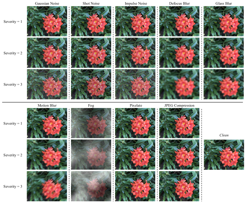
Figure 6: More image samples on LLFF-C

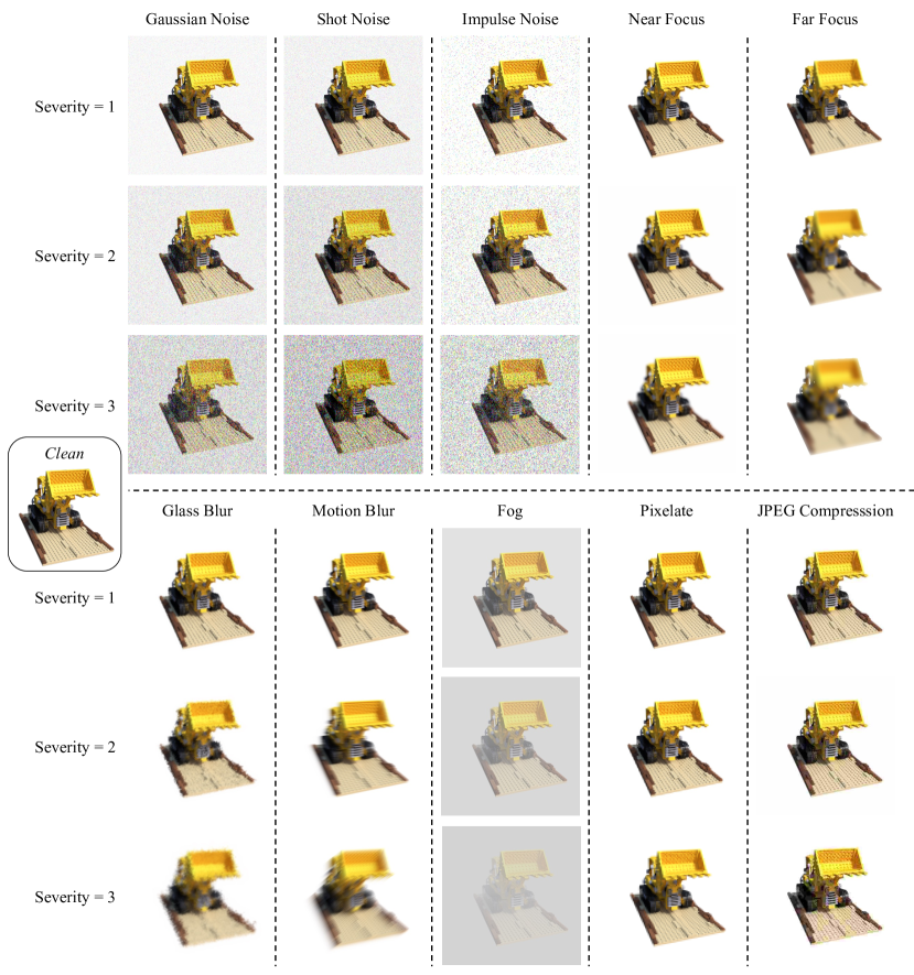
Figure 7: More image samples on LLFF-C

We construct LLFF-C at the resolution of $504\times 378$, and Blender-C at the resolution of $400\times 400$, mainly to save training time. See Figure 6 and Figure 7 for a full set of corruption examples.

Appendix C Details for Each Method

NeRF [24], MipNeRF [3] We trained scenes in both datasets for 200,000 iterations.

IBRNet [41] We fine-tuned each scene in the LLFF-C and Blender-C datasets for 45,000 steps and 15,000 steps respectively.

MVSNeRF [5] requires the height and width of the image resolution divisible by 32, so the inputs images in LLFF-C and Blender-C are resized to $480\times 320$ and $384\times 384$ respectively. The metric evaluation is done at the resized resolution. MVSNeRF uses 15 images for training and another 4 images for testing in the LLFF dataset, but we followed the original train-test split for LLFF as in the original NeRF. As for the Blender-C dataset, we use the target training set and target testing set partition in MVSNeRF since we found MVSNeRF performs badly on the standard one. We fine-tuned each scene for 1 epoch.

Plenoxel [7] We use the official code directly for optimization and evaluation.

GPNR [35] Since there is no official checkpoint available, we trained GPNR on the IBRNet collected dataset for 150,000 steps and tested it on LLFF-C.

Appendix D Encoder Architecture

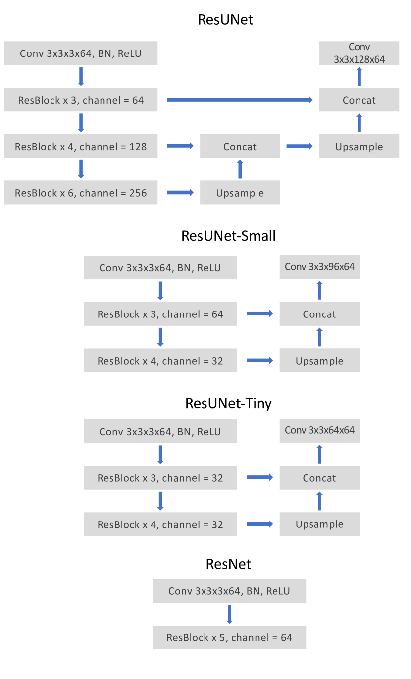
Figure 8: More image samples on LLFF-C

The feature encoders we experimented with for generalizable methods can be found in Figure 8.

		Noise			Blur			Weather	Digital
	Clean	Gauss.	Shot	Impulse	Defocus	Glass	Motion	Fog	Pixel	JPEG
NeRF (patch=2)	27.40/0.164	24.16/0.308	23.58/0.311	23.90/0.307	20.83/0.507	22.24/0.378	19.35/0.483	11.99/0.545	24.23/0.306	25.20/0.293
NeRF (patch=4)	26.92/0.184	23.98/0.313	23.45/0.317	23.78/0.312	20.84/0.512	22.19/0.385	19.47/0.489	11.89/0.635	23.31/0.299	24.99/0.301
MVSNeRF (patch=2)	23.24/0.267	21.13/0.457	20.84/0.458	21.06/0.457	20.36/0.523	21.29/0.425	19.24/0.504	13.35/0.610	22.23/0.373	22.61/0.368
MVSNeRF (patch=4)	22.74/0.285	20.73/0.470	20.51/0.469	20.70/0.470	20.07/0.536	20.89/0.442	19.00/0.516	13.53/0.614	21.78/0.389	22.09/0.385

Table 6: PSNR/LPIPS results for clean and corrupted data on LLFF-C, ft indicates results after fine-tuning for generalizable methods.

		Noise			Blur			Weather	Digital
	Clean	Gauss.	Shot	Impulse	Defocus	Glass	Motion	Fog	Pixel	JPEG
NeRF	0.876	0.769	0.773	0.768	0.521	0.661	0.498	0.398	0.750	0.797
MipNeRF	0.874	0.722	0.719	0.718	0.521	0.658	0.487	0.396	0.746	0.698
Plenoxel	0.900	0.481	0.481	0.458	0.529	0.659	0.527	0.249	0.747	0.788
MVSNeRF	0.629	0.546	0.543	0.542	0.549	0.588	0.523	0.487	0.616	0.613
MVSNeRF (ft)	0.842	0.735	0.743	0.736	0.645	0.729	0.635	0.510	0.777	0.806
IBRNet	0.844	0.572	0.575	0.598	0.508	0.637	0.516	0.473	0.722	0.748
IBRNet (ft)	0.893	0.745	0.577	0.740	0.491	0.631	0.517	0.429	0.685	0.766
GPNR	0.813	0.576	0.575	0.581	0.500	0.616	0.497	0.376	0.699	0.731

Table 7: SSIM results for clean and corrupted data on LLFF-C, ft indicates results after fine-tuning for generalizable methods.

		Noise			Blur				Weather	Digital
	Clean	Gauss.	Shot	Impulse	Near Focus	Far Focus	Glass	Motion	Fog	Pixel	JPEG
NeRF	0.952	0.919	0.912	0.918	0.912	0.881	0.832	0.812	0.836	0.906	0.925
MipNeRF	0.857	0.849	0.717	0.759	0.808	0.848	0.841	0.694	0.796	0.850	0.823
Plenoxel	0.966	0.445	0.338	0.538	0.928	0.896	0.828	0.811	0.750	0.904	0.923
MVSNeRF	0.857	0.849	0.717	0.759	0.808	0.848	0.841	0.694	0.796	0.850	0.823
MVSNeRF (ft)	0.883	0.806	0.781	0.874	0.818	0.876	0.877	0.782	0.805	0.879	0.850
IBRNet	0.926	0.667	0.587	0.616	0.896	0.867	0.820	0.815	0.824	0.889	0.898
IBRNet (ft)	0.951	0.685	0.635	0.631	0.893	0.857	0.835	0.817	0.816	0.878	0.875

Table 8: SSIM results for clean and corrupted data on Blender-C, ft indicates results after fine-tuning for generalizable methods.

		Noise			Blur			Weather	Digital
	Avg.	Gauss.	Shot	Impulse	Defocus	Glass	Motion	Fog	Pixel	JPEG
NeRF	0.21	0.12	0.14	0.13	0.25	0.31	0.20	0.57	0.12	0.09
MipNeRF	0.23	0.13	0.16	0.14	0.25	0.31	0.20	0.57	0.13	0.20
Plenoxel	0.27	0.25	0.26	0.35	0.26	0.30	0.20	0.55	0.13	0.10
MVSNeRF	0.05	0.01	0.03	0.02	0.01	0.04	0.02	0.24	0.04	0.02
MVSNeRF (ft)	0.14	0.10	0.12	0.11	0.14	0.19	0.10	0.45	0.05	0.03
IBRNet	0.19	0.15	0.17	0.14	0.20	0.25	0.15	0.47	0.09	0.07
IBRNet (ft)	0.24	0.14	0.23	0.14	0.29	0.30	0.21	0.52	0.18	0.11
GPNR	0.17	0.12	0.14	0.13	0.17	0.22	0.13	0.48	0.07	0.05

Table 9: RmCM results for PSNR on LLFF-C, ft indicates results after fine-tuning for generalizable methods.

		Noise			Blur			Weather	Digital
	Avg.	Gauss.	Shot	Impulse	Defocus	Glass	Motion	Fog	Pixel	JPEG
NeRF	0.25	0.12	0.12	0.12	0.41	0.25	0.43	0.55	0.14	0.09
MipNeRF	0.28	0.17	0.18	0.18	0.40	0.25	0.44	0.55	0.15	0.20
Plenoxel	0.39	0.47	0.47	0.49	0.41	0.27	0.41	0.72	0.17	0.12
MVSNeRF	0.12	0.13	0.14	0.14	0.13	0.07	0.17	0.23	0.02	0.03
MVSNeRF (ft)	0.17	0.13	0.12	0.13	0.23	0.13	0.25	0.39	0.08	0.04
IBRNet	0.30	0.32	0.32	0.29	0.40	0.25	0.39	0.44	0.15	0.11
IBRNet (ft)	0.31	0.17	0.35	0.17	0.45	0.29	0.42	0.52	0.23	0.14
GPNR	0.30	0.29	0.29	0.29	0.39	0.24	0.39	0.54	0.14	0.10

Table 10: RmCM results for SSIM on LLFF-C, ft indicates results after fine-tuning for generalizable methods.

		Noise			Blur			Weather	Digital
	Avg.	Gauss.	Shot	Impulse	Defocus	Glass	Motion	Fog	Pixel	JPEG
NeRF	1.48	0.97	0.99	0.97	2.36	1.46	2.20	2.50	1.00	0.91
MipNeRF	1.47	1.13	1.17	1.14	2.20	1.38	2.18	2.42	0.98	0.61
Plenoxel	3.50	3.80	3.86	3.94	4.08	2.72	3.63	5.59	1.88	2.00
MVSNeRF	0.29	0.33	0.35	0.35	0.41	0.22	0.36	0.39	0.10	0.14
MVSNeRF (ft)	0.84	0.81	0.81	0.81	1.11	0.67	1.01	1.48	0.45	0.43
IBRNet	1.67	1.86	1.88	1.75	2.25	1.48	1.87	1.87	0.97	1.14
IBRNet (ft)	2.57	1.85	3.01	1.87	3.59	2.51	3.05	3.46	2.03	1.77
GPNR	1.18	1.28	1.29	1.26	1.52	0.98	1.29	1.70	0.62	0.64

Table 11: RmCM results for LPIPS on LLFF-C, ft indicates results after fine-tuning for generalizable methods.

		Noise			Blur				Weather	Digital
	Avg.	Gauss.	Shot	Impulse	Near Focus	Far Focus	Glass	Motion	Fog	Pixel	JPEG
NeRF	0.26	0.29	0.38	0.23	0.13	0.20	0.27	0.33	0.50	0.13	0.09
MipNeRF	0.29	0.32	0.41	0.25	0.16	0.22	0.33	0.37	0.53	0.17	0.11
Plenoxel	0.31	0.38	0.46	0.32	0.16	0.22	0.32	0.36	0.53	0.19	0.13
MVSNeRF	0.12	0.02	0.27	0.20	0.12	0.01	0.03	0.21	0.28	0.02	0.07
MVSNeRF (ft)	0.15	0.24	0.31	0.03	0.19	0.02	0.02	0.22	0.38	0.01	0.08
IBRNet	0.20	0.25	0.33	0.21	0.08	0.12	0.20	0.24	0.44	0.08	0.06
IBRNet (ft)	0.28	0.30	0.33	0.25	0.17	0.24	0.28	0.33	0.49	0.20	0.20

Table 12: RmCM results for PSNR on Blender-C, ft indicates results after fine-tuning for generalizable methods.

		Noise			Blur				Weather	Digital
	Avg.	Gauss.	Shot	Impulse	Near Focus	Far Focus	Glass	Motion	Fog	Pixel	JPEG
NeRF	0.07	0.03	0.04	0.04	0.04	0.07	0.13	0.15	0.12	0.05	0.03
MipNeRF	0.07	0.01	0.16	0.11	0.06	0.01	0.02	0.19	0.07	0.01	0.04
Plenoxel	0.24	0.54	0.65	0.44	0.04	0.07	0.14	0.16	0.22	0.06	0.04
MVSNeRF	0.07	0.01	0.16	0.11	0.06	0.01	0.02	0.19	0.07	0.01	0.04
MVSNeRF (ft)	0.05	0.09	0.12	0.01	0.07	0.01	0.01	0.11	0.09	0.01	0.04
IBRNet	0.15	0.28	0.37	0.34	0.03	0.06	0.11	0.12	0.11	0.04	0.03
IBRNet (ft)	0.17	0.28	0.33	0.34	0.06	0.10	0.12	0.14	0.14	0.08	0.08

Table 13: RmCM results for SSIM on Blender-C, ft indicates results after fine-tuning for generalizable methods.

		Noise			Blur				Weather	Digital
	Avg.	Gauss.	Shot	Impulse	Near Focus	Far Focus	Glass	Motion	Fog	Pixel	JPEG
NeRF	1.41	1.29	1.91	1.34	0.78	1.21	1.94	2.26	1.81	0.93	0.63
MipNeRF	1.58	1.44	2.45	1.91	0.62	0.99	2.40	2.47	2.01	0.92	0.60
Plenoxel	7.51	14.82	16.16	12.11	1.85	2.29	4.96	5.40	12.56	2.70	2.26
MVSNeRF	0.46	0.08	1.10	0.94	0.26	0.10	0.12	1.08	0.62	0.09	0.24
MVSNeRF (ft)	0.73	1.58	1.82	0.05	0.53	0.11	0.09	1.70	1.04	0.09	0.28
IBRNet	1.13	2.43	2.75	2.49	0.01	0.48	0.89	0.78	0.66	0.39	0.39
IBRNet (ft)	2.48	4.96	5.12	5.04	0.55	1.43	1.50	1.60	2.16	1.18	1.30

Table 14: RmCM results for LPIPS on Blender-C, ft indicates results after fine-tuning for generalizable methods.

References

- [1] Kara-Ali Aliev, Artem Sevastopolsky, Maria Kolos, Dmitry Ulyanov, and Victor Lempitsky. Neural point-based graphics. In European Conference on Computer Vision, pages 696–712. Springer, 2020.
- [2] Andrei Barbu, David Mayo, Julian Alverio, William Luo, Christopher Wang, Dan Gutfreund, Josh Tenenbaum, and Boris Katz. Objectnet: A large-scale bias-controlled dataset for pushing the limits of object recognition models. Advances in neural information processing systems, 32, 2019.
- [3] Jonathan T Barron, Ben Mildenhall, Matthew Tancik, Peter Hedman, Ricardo Martin-Brualla, and Pratul P Srinivasan. Mip-nerf: A multiscale representation for anti-aliasing neural radiance fields. In Proceedings of the IEEE/CVF International Conference on Computer Vision, pages 5855–5864, 2021.
- [4] Prithvijit Chattopadhyay, Judy Hoffman, Roozbeh Mottaghi, and Aniruddha Kembhavi. Robustnav: Towards benchmarking robustness in embodied navigation. In Proceedings of the IEEE/CVF International Conference on Computer Vision, pages 15691–15700, 2021.
- [5] Anpei Chen, Zexiang Xu, Fuqiang Zhao, Xiaoshuai Zhang, Fanbo Xiang, Jingyi Yu, and Hao Su. Mvsnerf: Fast generalizable radiance field reconstruction from multi-view stereo. In Proceedings of the IEEE/CVF International Conference on Computer Vision, pages 14124–14133, 2021.
- [6] Tianlong Chen, Peihao Wang, Zhiwen Fan, and Zhangyang Wang. Aug-nerf: Training stronger neural radiance fields with triple-level physically-grounded augmentations. In Proceedings of the IEEE/CVF Conference on Computer Vision and Pattern Recognition, pages 15191–15202, 2022.
- [7] Sara Fridovich-Keil, Alex Yu, Matthew Tancik, Qinhong Chen, Benjamin Recht, and Angjoo Kanazawa. Plenoxels: Radiance fields without neural networks. In Proceedings of the IEEE/CVF Conference on Computer Vision and Pattern Recognition, pages 5501–5510, 2022.
- [8] Steven J Gortler, Radek Grzeszczuk, Richard Szeliski, and Michael F Cohen. The lumigraph. In Proceedings of the 23rd annual conference on Computer graphics and interactive techniques, pages 43–54, 1996.
- [9] Peter Hedman, Julien Philip, True Price, Jan-Michael Frahm, George Drettakis, and Gabriel Brostow. Deep blending for free-viewpoint image-based rendering. ACM Transactions on Graphics (TOG), 37(6):1–15, 2018.
- [10] Peter Hedman, Tobias Ritschel, George Drettakis, and Gabriel Brostow. Scalable inside-out image-based rendering. ACM Transactions on Graphics (TOG), 35(6):1–11, 2016.
- [11] Dan Hendrycks, Steven Basart, Norman Mu, Saurav Kadavath, Frank Wang, Evan Dorundo, Rahul Desai, Tyler Zhu, Samyak Parajuli, Mike Guo, et al. The many faces of robustness: A critical analysis of out-of-distribution generalization. In Proceedings of the IEEE/CVF International Conference on Computer Vision, pages 8340–8349, 2021.
- [12] Dan Hendrycks and Thomas Dietterich. Benchmarking neural network robustness to common corruptions and perturbations. arXiv preprint arXiv:1903.12261, 2019.
- [13] Dan Hendrycks, Norman Mu, Ekin D Cubuk, Barret Zoph, Justin Gilmer, and Balaji Lakshminarayanan. Augmix: A simple data processing method to improve robustness and uncertainty. arXiv preprint arXiv:1912.02781, 2019.
- [14] Dan Hendrycks, Kevin Zhao, Steven Basart, Jacob Steinhardt, and Dawn Song. Natural adversarial examples. In Proceedings of the IEEE/CVF Conference on Computer Vision and Pattern Recognition, pages 15262–15271, 2021.
- [15] James T Kajiya and Brian P Von Herzen. Ray tracing volume densities. ACM SIGGRAPH computer graphics, 18(3):165–174, 1984.
- [16] Nima Khademi Kalantari, Ting-Chun Wang, and Ravi Ramamoorthi. Learning-based view synthesis for light field cameras. ACM Transactions on Graphics (TOG), 35(6):1–10, 2016.
- [17] Oğuzhan Fatih Kar, Teresa Yeo, Andrei Atanov, and Amir Zamir. 3d common corruptions and data augmentation. In Proceedings of the IEEE/CVF Conference on Computer Vision and Pattern Recognition, pages 18963–18974, 2022.
- [18] Marc Levoy and Pat Hanrahan. Light field rendering. In Proceedings of the 23rd annual conference on Computer graphics and interactive techniques, pages 31–42, 1996.
- [19] William E Lorensen and Harvey E Cline. Marching cubes: A high resolution 3d surface construction algorithm. ACM siggraph computer graphics, 21(4):163–169, 1987.
- [20] Li Ma, Xiaoyu Li, Jing Liao, Qi Zhang, Xuan Wang, Jue Wang, and Pedro V Sander. Deblur-nerf: Neural radiance fields from blurry images. In Proceedings of the IEEE/CVF Conference on Computer Vision and Pattern Recognition, pages 12861–12870, 2022.
- [21] Aleksander Madry, Aleksandar Makelov, Ludwig Schmidt, Dimitris Tsipras, and Adrian Vladu. Towards deep learning models resistant to adversarial attacks. arXiv preprint arXiv:1706.06083, 2017.
- [22] Ben Mildenhall, Peter Hedman, Ricardo Martin-Brualla, Pratul P Srinivasan, and Jonathan T Barron. Nerf in the dark: High dynamic range view synthesis from noisy raw images. In Proceedings of the IEEE/CVF Conference on Computer Vision and Pattern Recognition, pages 16190–16199, 2022.
- [23] Ben Mildenhall, Pratul P Srinivasan, Rodrigo Ortiz-Cayon, Nima Khademi Kalantari, Ravi Ramamoorthi, Ren Ng, and Abhishek Kar. Local light field fusion: Practical view synthesis with prescriptive sampling guidelines. ACM Transactions on Graphics (TOG), 38(4):1–14, 2019.
- [24] Ben Mildenhall, Pratul P Srinivasan, Matthew Tancik, Jonathan T Barron, Ravi Ramamoorthi, and Ren Ng. Nerf: Representing scenes as neural radiance fields for view synthesis. In European conference on computer vision, pages 405–421. Springer, 2020.
- [25] Michael Niemeyer and Andreas Geiger. Giraffe: Representing scenes as compositional generative neural feature fields. In Proceedings of the IEEE/CVF Conference on Computer Vision and Pattern Recognition, pages 11453–11464, 2021.
- [26] Naama Pearl, Tali Treibitz, and Simon Korman. Nan: Noise-aware nerfs for burst-denoising. In Proceedings of the IEEE/CVF Conference on Computer Vision and Pattern Recognition, pages 12672–12681, 2022.
- [27] Eric Penner and Li Zhang. Soft 3d reconstruction for view synthesis. ACM Transactions on Graphics (TOG), 36(6):1–11, 2017.
- [28] Benjamin Recht, Rebecca Roelofs, Ludwig Schmidt, and Vaishaal Shankar. Do imagenet classifiers generalize to imagenet? In International Conference on Machine Learning, pages 5389–5400. PMLR, 2019.
- [29] Jiawei Ren, Liang Pan, and Ziwei Liu. Benchmarking and analyzing point cloud classification under corruptions. arXiv preprint arXiv:2202.03377, 2022.
- [30] Gernot Riegler and Vladlen Koltun. Free view synthesis. In European Conference on Computer Vision, pages 623–640. Springer, 2020.
- [31] Gernot Riegler and Vladlen Koltun. Stable view synthesis. In Proceedings of the IEEE/CVF Conference on Computer Vision and Pattern Recognition, pages 12216–12225, 2021.
- [32] Darius Rückert, Linus Franke, and Marc Stamminger. Adop: Approximate differentiable one-pixel point rendering. ACM Transactions on Graphics (TOG), 41(4):1–14, 2022.
- [33] Johannes L Schonberger and Jan-Michael Frahm. Structure-from-motion revisited. In Proceedings of the IEEE conference on computer vision and pattern recognition, pages 4104–4113, 2016.
- [34] Pratul P Srinivasan, Richard Tucker, Jonathan T Barron, Ravi Ramamoorthi, Ren Ng, and Noah Snavely. Pushing the boundaries of view extrapolation with multiplane images. In Proceedings of the IEEE/CVF Conference on Computer Vision and Pattern Recognition, pages 175–184, 2019.
- [35] Mohammed Suhail, Carlos Esteves, Leonid Sigal, and Ameesh Makadia. Generalizable patch-based neural rendering. arXiv preprint arXiv:2207.10662, 2022.
- [36] Justus Thies, Michael Zollhöfer, and Matthias Nießner. Deferred neural rendering: Image synthesis using neural textures. ACM Transactions on Graphics (TOG), 38(4):1–12, 2019.
- [37] Angtian Wang, Peng Wang, Jian Sun, Adam Kortylewski, and Alan Yuille. Voge: A differentiable volume renderer using gaussian ellipsoids for analysis-by-synthesis. arXiv preprint arXiv:2205.15401, 2022.
- [38] Chen Wang, Xian Wu, Yuan-Chen Guo, Song-Hai Zhang, Yu-Wing Tai, and Shi-Min Hu. Nerf-sr: High quality neural radiance fields using supersampling. In Proceedings of the 30th ACM International Conference on Multimedia, pages 6445–6454, 2022.
- [39] Dilin Wang, Chengyue Gong, and Qiang Liu. Improving neural language modeling via adversarial training. In International Conference on Machine Learning, pages 6555–6565. PMLR, 2019.
- [40] Peng Wang, Lingjie Liu, Yuan Liu, Christian Theobalt, Taku Komura, and Wenping Wang. Neus: Learning neural implicit surfaces by volume rendering for multi-view reconstruction. arXiv preprint arXiv:2106.10689, 2021.
- [41] Qianqian Wang, Zhicheng Wang, Kyle Genova, Pratul P Srinivasan, Howard Zhou, Jonathan T Barron, Ricardo Martin-Brualla, Noah Snavely, and Thomas Funkhouser. Ibrnet: Learning multi-view image-based rendering. In Proceedings of the IEEE/CVF Conference on Computer Vision and Pattern Recognition, pages 4690–4699, 2021.
- [42] Zhou Wang, Eero P Simoncelli, and Alan C Bovik. Multiscale structural similarity for image quality assessment. In The Thrity-Seventh Asilomar Conference on Signals, Systems & Computers, 2003, volume 2, pages 1398–1402. Ieee, 2003.
- [43] Yi Wei, Shaohui Liu, Yongming Rao, Wang Zhao, Jiwen Lu, and Jie Zhou. Nerfingmvs: Guided optimization of neural radiance fields for indoor multi-view stereo. In Proceedings of the IEEE/CVF International Conference on Computer Vision, pages 5610–5619, 2021.
- [44] Cihang Xie, Mingxing Tan, Boqing Gong, Jiang Wang, Alan L Yuille, and Quoc V Le. Adversarial examples improve image recognition. In Proceedings of the IEEE/CVF Conference on Computer Vision and Pattern Recognition, pages 819–828, 2020.
- [45] Yiheng Xie, Towaki Takikawa, Shunsuke Saito, Or Litany, Shiqin Yan, Numair Khan, Federico Tombari, James Tompkin, Vincent Sitzmann, and Srinath Sridhar. Neural fields in visual computing and beyond. In Computer Graphics Forum, volume 41, pages 641–676. Wiley Online Library, 2022.
- [46] Lior Yariv, Yoni Kasten, Dror Moran, Meirav Galun, Matan Atzmon, Basri Ronen, and Yaron Lipman. Multiview neural surface reconstruction by disentangling geometry and appearance. Advances in Neural Information Processing Systems, 33:2492–2502, 2020.
- [47] Alex Yu, Vickie Ye, Matthew Tancik, and Angjoo Kanazawa. pixelnerf: Neural radiance fields from one or few images. In Proceedings of the IEEE/CVF Conference on Computer Vision and Pattern Recognition, pages 4578–4587, 2021.
- [48] Sangdoo Yun, Dongyoon Han, Seong Joon Oh, Sanghyuk Chun, Junsuk Choe, and Youngjoon Yoo. Cutmix: Regularization strategy to train strong classifiers with localizable features. In Proceedings of the IEEE/CVF international conference on computer vision, pages 6023–6032, 2019.
- [49] Hongyi Zhang, Moustapha Cisse, Yann N Dauphin, and David Lopez-Paz. mixup: Beyond empirical risk minimization. arXiv preprint arXiv:1710.09412, 2017.
- [50] Richard Zhang, Phillip Isola, Alexei A Efros, Eli Shechtman, and Oliver Wang. The unreasonable effectiveness of deep features as a perceptual metric. In Proceedings of the IEEE conference on computer vision and pattern recognition, pages 586–595, 2018.
- [51] Tinghui Zhou, Richard Tucker, John Flynn, Graham Fyffe, and Noah Snavely. Stereo magnification: Learning view synthesis using multiplane images. arXiv preprint arXiv:1805.09817, 2018.