Modeling the vertical distribution of the Milky Way’s flat subsystem objects

Abstract

This paper is an initial stage of consideration of the general problem of joint modeling of the vertical structure of a Galactic flat subsystem and the average surface of the disk of the Galaxy, taking into account the natural and measurement dispersions. We approximate the average surface of the Galactic disk in the region covered by the data with a general (polynomial) model and determine its parameters by minimizing the squared deviations of objects along the normal to the model surface. The smoothness of the model, i.e., its order $n$, is optimized. An outlier elimination algorithm is applied. The developed method allows us to simultaneously identify significant details of the Galactic warping and estimate the offset $z_{\sun}$ of the Sun relative to the average (in general, non-flat) surface of the Galactic disk and the vertical scale of the object system under consideration for an arbitrary area of the disk covered by data. The method is applied to data on classical Cepheids (Berdnikov et al., Mel’nik et al.). Significant local extremes of the average disk surface model were found based on Cepheid data: the minimum in the first Galactic quadrant and the maximum in the second. A well-known warp (lowering of the disk surface) in the third quadrant has been confirmed. The optimal order of the model describing all these warping details was found to be $n_{\text{o}}=4$. The local (for a small neighborhood of the Sun, $n_{\text{o}}=0$) estimate of $z_{\sun}=28.1\pm\left.6.1\right|_{\text{stat.}}\left.{}\pm 1.3\right|_{\text{cal.}}$ pc is close to the non-local (taking into account warping, $n_{\text{o}}=4$) $z_{\sun}=27.1\pm\left.8.8\right|_{\text{stat.}}\left.{}^{+1.3}_{-1.2}\right|_{\text{cal.}}$ pc (statistical and calibration uncertainties are indicated), which suggests that the proposed modeling method eliminates the influence of warping on the $z_{\sun}$ estimate. However, the non-local estimate of the vertical standard deviation of Cepheids $\sigma_{\rho}=132.0\pm\left.3.7\right|_{\text{stat.}}\left.{}^{+6.3}_{-5.9}\right|_{\text{cal.}}$ pc differs significantly from the local $\sigma_{\rho}=\left.76.5\pm 4.4\right|_{\text{stat.}}\left.{}^{+3.6}_{-3.4}\right|_{\text{cal.}}$  pc, which means the need to introduce more complex models for the vertical distribution outside the Sun’s vicinity.

1 Introduction

The vertical distribution of objects in various Galactic subsystems contains valuable information about the origin, evolution and dynamics of our Galaxy, so determining the characteristics of this distribution is an important task of Galactic Astronomy. The study of the vertical distribution may include consideration of many phenomena, but one of them should be taken into account necessarily—this is the offset $z_{\sun}$ of the Sun relative to the plane of the Milky Way’s disk towards the North Galactic Pole. Therefore, in the simplest case, modeling of the vertical distribution is reduced to determining the value of $z_{\sun}$ and some dispersion parameter (standard deviation, scale height, etc.) that characterizes the scattering of subsystem objects relative to the average plane of the Galactic disk (usually relative to the midplane of this subsystem). The first estimate of $z_{\sun}=13.5\pm 1.7\,\text{pc}$ was obtained by van Tulder (1942) from the analysis of nearby stars. Subsequently, in many papers, the solar offset was determined by different methods for various objects and Galactic subsystems. Bland-Hawthorn & Gerhard (2016) adopted as the best (local) estimate the result of Jurić et al. (2008) from the complete SDSS photometric survey, $z_{\sun}=25\pm 5\,\text{pc}$, which covers many other estimates.

However, the solar offset relative to the differently defined midplane of the disk does not seem to be described by a single value of $z_{\sun}$. For example, Bobylev & Bajkova (2016b) obtained significantly different results for reference objects (tracers) of different types: $z_{\sun}=5.7\pm 0.5$ pc for a sample of methanol masers, $z_{\sun}=7.6\pm 0.4$ pc for data on H II regions and $z_{\sun}=10.1\pm 0.5$ pc for data on giant molecular clouds; at the same time, Ferguson et al. (2017) derived values of $z_{\sun}=14.9\pm 0.5$ pc for a uniform selection of SDSS K and M dwarf stars and $z_{\sun}=15.3\pm 0.4$ pc for an expanded selection, Buckner & Froebrich (2014) found an estimate $z_{\sun}=18.5\pm 1.2\,\text{pc}$ for open clusters, and Majaess et al. (2009) obtained values of $z_{\sun}=26\pm 3$ pc for Cepheids. A comparison of these and other $z_{\sun}$ estimates obtained in various studies (see, e.g., summaries in Yao et al. 2017; Skowron et al. 2019a) shows that the differences between these estimates cannot be explained only by statistical errors, with some estimates varing significantly, even for objects of the same type (e.g., for open clusters and Cepheids). This shows that the discrepancies reflect not only the possible objective difference in the values of $z_{\sun}$ between different types of objects (subsystems of the Galaxy), but also other factors in the problem.

In addition to the $Z$-offset of the Sun, the number of already established or potential factors affecting the results of modeling the vertical distribution of objects includes: 1) the warp of the Galactic disk, 2) the dependence of the values of the characteristics of the vertical distribution on the position on the disk for the selected Galactic subsystem (e.g., the flare of the Galactic disk), 3) the possible (and in the case of vertical dispersion, real) dependence of these characteristics on the type of Galactic subsystem, 4) the need to establish the functional type of the vertical distribution and its possible variations with the position on the disk and with the type of subsystem, as well as 5) taking into account the random uncertainty of heliocentric distances, systematically distorting the true vertical distribution. The problem in general (taking into account all these factors) has not yet been solved. Meanwhile, different combinations of these factors may be responsible for discrepancy of the results (in particular, of $z_{\sun}$ estimates) in different papers. Subjective factors can also lead to this: the choice of the general appearance of the model of the average surface of the disk, possible mismatch of the distance scales used in different works, the dependence of the results of modeling on the size and configuration of the disk area under consideration (the area covered by the data).

Despite the lack of a solution to the problem in general, some of these factors and their combinations were considered. The most important factor is the presence of a warp of the Milky Way’s disk. The warp was noticed as soon as the observation data in the 21-cm line of neutral hydrogen appeared for the southern hemisphere (Burke 1957; Kerr 1957). Subsequent studies (Oort et al. 1958; see, e.g., Binney & Merrifield 1998 and Bland-Hawthorn & Gerhard 2016 reviews and references therein; Skowron et al. 2019a; Chrobáková et al. 2020, among others) have shown that a significant stellar/gas warp begins outside the solar circle, and in the inner Galaxy the disk is very close to flat, including on the far side of the disk (Minniti et al. 2021). Various data indicate that one part of the warped disk deviates from the plane of the inner disk towards the North Galactic Pole, the other deviates in the opposite direction.

Not taking into account the large-scale warp (if a plane parallel to the equator of the Galactic coordinate system $b=0^{\circ}$ is taken as a model of the average surface of the Galactic disk) can significantly affect the estimates of the solar offset $z_{\sun}$ and the vertical scales of flat subsystems (see, e.g., the dependence of these characteristics for planetary nebulae on the size of considered near-solar region in Bobylev & Bajkova 2017). One way to avoid this is to exclude the warp zone from consideration under the assumption that in the remaining area of the disk its average surface is flat: restrictions are imposed on the selection of tracers, for example, by the heliocentric distances $r$ (e.g., $r\lesssim 4$ kpc in Bobylev & Bajkova 2016a; $r\lesssim 4.5$ kpc in Bobylev & Bajkova 2016b), by the predicted maximum warp offsets (${<}10$ pc in Yao et al. 2017), by the distance $R$ to the axis of rotation of the Galaxy ($R<7.0$ kpc in Reid et al. 2019). However, the exclusion of the warp zone requires the adoption of a specific warp model, and it is often taken simple for this and other applications: the disk in the inner Galaxy ($R\leq R_{\text{w}}$) is considered undisturbed, and in the outer one ($R>R_{\text{w}}$) it is usually represented by a combination of a power dependence on $R$ and a simple trigonometric function of the azimuthal coordinate (e.g., Binney & Merrifield 1998; Pohl et al. 2008; Xu et al. 2015; Yao et al. 2017; Romero-Gómez et al. 2019; Cheng et al. 2020; Mosenkov et al. 2021). At the same time, to describe the warp in the outer Galaxy, in most of its morphological studies, simple symmetric models with a limited set of parameters are used—the radius $R_{\text{w}}$ at which the disk starts bending, the phase angle of the line-of-nodes and the maximum amplitude of the warp (see, e.g., Romero-Gómez et al. 2019 and references therein).

However, the warp is clearly more complicated. Firstly, the inner part of the disk is not perfectly flat— there are corrugations on the scale of ${\sim}30$ pc (Oort et al. 1958, fig. 3; Spicker & Feitzinger 1986; Binney & Merrifield 1998, fig. 9.22). $N$-body simulations of the Milky Way interacting with a satellite similar to the Sagittarius dwarf galaxy show that repeated satellite passes can generate local ripples, including in the inner disk (Poggio et al. 2020, fig. 2). According to kinematics, the onset of the warp occurs at a guiding radius inside the Solar circle, $R_{\text{g}}\lesssim 7$ kpc (Schoenrich & Dehnen 2018), or even in the center of the Galaxy (Li et al. 2020). Secondly, the outer part of the warp is also not described by a simple model—there are manifestations of lopsidedness of the warp and twisting of its line-of-nodes (Romero-Gómez et al. 2019; Chrobáková et al. 2020); Xu et al. (2015) detected an oscillating asymmetry in the SDSS main-sequence star counts on either side of the Galactic plane in the anticenter region, between longitudes of $110^{\circ}<l<229^{\circ}$. In addition, the morphology and kinematics of the warp depend on the type/age of the tracers (e.g., Romero-Gómez et al. 2019; Chrobáková et al. 2020). Moreover, hydrodynamic modeling of the evolution of an ensemble of stars formed in the warp shows that only younger populations trace the warp detected by HI (Khachaturyants et al. 2021) and that the influence of the bending waves excited by irregular gas inflow is most strongly manifested in the young populations (Khachaturyants et al. 2022). This means that the warp model, universal for all disk subsystems of the Galaxy, can hardly be accepted.

Kinematic manifestations of the warp also indicate its asymmetry and complexity in general, as well as the dependence of its characteristics on the age of tracers (e.g., Romero-Gómez et al. 2019; Li et al. 2020; Cheng et al. 2020 and references in these works).

Based on the above, the exclusion of the warp zone as a method of eliminating biases in the vertical distribution parameters can only give a partial (local) solution to the problem, the accuracy of which depends on the details of the accepted warp model and on its realism in the case of the tracers under consideration and on assumptions about the boundaries of the warp-distorted area. All these assumptions can be sources of systematic errors. That is why it seems important to us to abandon simplified warp models and consider the most general analytical warp model describing all the significant structural features of the middle surface of the disk identified by the tracers under consideration. The method of excluding the warp zone is also unsuccessful due to the presence of the disk flaring, which begins at $R\gtrsim R_{0}$, where $R_{0}$ is the Galactic center distance (e.g., Reid et al. 2019; Mosenkov et al. 2021), since the dependence of the dispersion parameter on the accepted boundaries of the area “undisturbed” by the warp appears.

The warp is currently being actively explored in many ways. In particular, warp precession is actively discussed (e.g., Cheng et al. 2020). However, as noted by Poggio et al. (2020), the precession parameters depend on our knowledge of the shape of the warp and its differences for different stellar populations. In addition, Chrobáková & López-Corredoira (2021) even raise the question of the very existence of precession, since the application of a warp model inconsistent with the tracers used leads to a fictitious precession.

Detailed warp models are also important both for studying the dependence of $z_{\sun}$ and vertical dispersion characteristics on the type/age of tracers, and for identifying the cause and dynamic nature of the warp of our Galaxy, which remain unclear (Binney & Merrifield 1998; Poggio et al. 2020; Khachaturyants et al. 2021).

Note also that in the framework of an alternative approach applied by Mosenkov et al. (2021)— photometric 3D decomposition of the Milky Way taking into account flaring and warp—the parameters of the warp disk are poorly determined, since only a 2D map is considered, whereas for creating a reliable 3D model of the warp one needs to have a 3D distribution of stars in the Galaxy.

Despite the fact that the best solution would be to model the $Z$-distribution of objects taking into account all the factors mentioned at once, due to the complexity of the overall task we focus in this paper on the task of constructing a detailed warp model with a minimum of assumptions. We will not consider the influence of random errors in the distance here (the selected data catalog allows this, see Sect. 3), as well as the disk flaring, since without taking into account errors in distances, the flaring parameters may turn out to be strongly biased.

2 Method

We will study the spatial distribution of objects in the heliocentric Cartesian coordinate system, which does not require taking any value of $R_{0}$: $X$-axis is directed towards the Galactic center, $Y$-axis is towards the rotation of the Galaxy, $Z$-axis is towards the North Galactic Pole.

In order to free the warp model as much as possible from pre-accepted assumptions, we will consider as models the $\zeta_{n}(X,Y)$ polynomials, each of which is a Maclaurin series expansion in the solar neighborhood up to the $n$-th order of the average $Z$-coordinate of the Galactic disk as a function of position on the $XY$ plane:

$$\begin{split}\zeta_{n}(X,Y)&=\sum_{i=0}^{n}{\sum_{j=0}^{i}{z_{i-j,\,j}X^{i-j}Y^{j}}}\\ &=z_{00}+z_{10}X+z_{01}Y+z_{20}X^{2}+z_{11}XY+z_{02}Y^{2}+\>\ldots\>+z_{n0}X^{n}+\>\ldots\>+z_{0n}Y^{n},\end{split}$$ (1)

$$\mathbf{z}_{\zeta}=\big{\{}z_{ij}\big{\}}_{0\,0}^{n\,i}\,,\quad\quad z_{\sun}=-z_{00}.$$

Here $\mathbf{z}_{\zeta}$ is the vector of $M=(n+2)(n+1)/2$ parameters of the model. Function (1) represents the average surface of the Galactic disk, defined by the spatial distribution of objects (in the general case of matter) of the selected Galactic subsystem. The distance $\rho$ from the object to the surface $\zeta_{n}(R,Z)$ along the normal to this surface will be considered as the value of the deviation of the object from the model average surface of the disk.

To obtain an estimate of the vector $\mathbf{z}_{\zeta}$, we generally use the maximum likelihood method. In this paper, to simplify, we assume that $\rho$ as a random variable is distributed according to a normal law with zero mean, that is, that the probability density of $\rho$ has the form

$$f(\rho)=\frac{1}{\sigma_{\rho}\sqrt{2\pi}}\ e^{-\frac{\rho^{2}}{2\sigma_{\rho}^{2}}},$$ (2)

where $\sigma_{\rho}$ is the standard deviation. We assume that the value of $\sigma_{\rho}$ is the same for all objects in the sample. However, in future work we propose to investigate and take into account the dependence of $\sigma_{\rho}$ and/or other dispersion parameters on the Galactocentric distance. With probability density (2), the likelihood function $L$ and logarithmic likelihood function $\cal L$ are

$$L=\prod\limits_{i=1}^{N}\frac{1}{\sigma_{\rho}\sqrt{2\pi}}\,e^{-\frac{\rho_{i}^{2}}{2\sigma_{\rho}^{2}}},$$

$${\cal L}\equiv-\ln{L}=\frac{N}{2}\ln{(2\pi)}+N\ln{\sigma_{\rho}}+\frac{1}{2}\sum\limits_{i=1}^{N}\frac{\rho_{i}^{2}}{\sigma_{\rho}^{2}}\,,$$ (3)

$$\rho_{i}=\rho_{i}(r_{i},l_{i},b_{i};\mathbf{z}_{\zeta}),$$

where $N$ is the number of objects in the sample; $r_{i}$, $l_{i}$ and $b_{i}$ are the heliocentric distance, galactic longitude and latitude of $i$-th object, correspondingly. Being a dispersion parameter under parametrization (2), $\sigma_{\rho}$ is included in the general vector of the problem parameters $\mathbf{z}=(\sigma_{\rho},\mathbf{z}_{\zeta})=(z_{1},z_{2},\>\ldots,\>z_{K})$, where $K=M+1$. The minimum of the function $\cal L$ gives estimates of the parameters, including the value of the standard deviation $\sigma_{\rho}$ of objects across the disk, which represents the contributions of both the true (natural) vertical dispersion of objects and the random uncertainty of distance estimates (the latter contribution is negligible, see Section 5). Thus, under assumption (2), the maximum likelihood method was reduced to the nonlinear least squares method (Eq. (3)). The resulting value of $\sigma_{\rho}$ was multiplied by the coefficient $\sqrt{N/(N-M)}$ to obtain an unbiased estimate. The vector $\mathbf{z}_{\text{err}}$ of mean parameter errors and the mean model prediction error $\sigma_{\zeta_{n}}(X,Y)$ were calculated based on the Hessian $H({\cal L})$ with elements $h_{ij}$ (Hudson 1964; Wall & Jenkins 2012):

$$\begin{gathered}h_{ij}=\frac{\partial{\cal L}^{2}}{\partial{z}_{i}\partial{z}_{j}}\,,\enskip i=1,\>\ldots,\>K,\enskip j=1,\>\ldots,\>K,\qquad C=[H({\cal L})]^{-1},\\ \mathbf{z}_{\text{err}}=\left\{\sqrt{c_{ii}}\right\}_{i=1}^{K}\,,\quad\sigma^{2}_{\zeta_{n}}(X,Y)=\{\mathop{\rm grad}\nolimits[\zeta_{n}(X,Y;\mathbf{z}_{\zeta})]\}^{\text{T}}\,C^{\prime}\,\mathop{\rm grad}\nolimits[\zeta_{n}(X,Y;\mathbf{z}_{\zeta})],\end{gathered}$$ (4)

where $c_{ii}$ are diagonal elements of the covariance matrix $C$, $C^{\prime}$ is a submatrix of $C$ that does not contain covariances involving $\sigma_{\rho}$; here, an estimate of the vector $\mathbf{z}$ obtained by minimizing ${\cal L}$ is substituted for all values.

After finding the parameters, an outlier exclusion algorithm described in Nikiforov (2012) was applied to the sample of objects under consideration. This algorithm differs from the usual $3\sigma$ criterion in that it uses a variable exclusion limit, which increases as the number of objects increases.

In order to check how well the observed distribution of sample objects by deviations $\rho$ agrees with the model probability density function (2), we use Pearson’s chi-square test.

A priori choice of the order $n$ of expansion (1) would lead to significant errors in all parameters, including $z_{00}$ (see Sect. 4), so the value of $n$ was also optimized using a simple algorithm. Models of the order $n=0$, 1, 2 and so on are built sequentially. For each model of order $n$, the number of parameters $z_{ij}$ of order $n$ ($i+j=n$) whose estimates differ from zero at the significance level ${\geq}2\sigma$ ($\sigma_{z_{ij}}/|z_{ij}|\leq 0.5$) is calculated. Then we find a model of the highest order such that it has at least one $2\sigma$-significant parameter of the same order as the model. If the total number of significant parameters of the selected model is greater than the corresponding number for any lower-order model, then the selected model of order $n$ is assumed to be optimal. Otherwise, a model of order $n-1$ is considered as possibly optimal and is compared in the same way with models of lower orders in terms of the number of significant parameters. Then either the order $n-1$ is assumed to be optimal, or a transition is made to the order $n-2$, and so on until some order $n\geq 0$ is accepted as optimal, $n_{\text{o}}$. The importance of choosing the correct model order will be illustrated in Section 4.

3 Data

We use the catalog of classical Cepheids by Berdnikov et al. (2000) in the version of Mel’nik et al. (2015), which provides data for 674 Cepheids from the General Catalogue of Variable Stars (e.g., Samus et al. 2017). The catalog is an updated version of the catalog of Cepheid parameters by Berdnikov et al. (2000). Observational data were obtained with 0.4–1 m telescopes of the Maidanak Observatory (Republic of Uzbekistan), Cerro Tololo and Las Campanas observatories (Chile), Cerro Armazones Observatory of the Catholic University (Chile) and South African Astronomical Observatory (see Dambis et al. 2015 for details). In particular, in order to reliably determine the distances, Cepheids discovered during the CCD monitoring of the southern sky performed as a part of the All Sky Automated Survey (ASAS) project (Pojmanski 2002) were observed, therefore, a survey of Cepheids across the entire sky was performed. The peak of the distribution of Cepheids by the mean apparent magnitudes in the $V$ band falls on the values of $\langle V\rangle=12$–$13$ mag, the limiting magnitude of the catalog is $\langle V\rangle=15$ mag. The distances were obtained based on the period–luminosity relation in the $K$ infrared band and interstellar-extinction law using the period – normal color $(B-V)$ relation derived earlier (see Dambis et al. 2015).

The authors of the catalog did not specify the possible value of the distance modulus error. However, the analysis of these data in Veselova & Nikiforov (2020) showed that the nominal random errors of distance estimates given in Mel’nik et al. (2015) are small (the mean error of distance moduli $\sigma_{d}<0.14^{m}$). Using this distance catalog gives us the opportunity to apply a simpler method that does not take into account random distance errors. In the future, we intend to use newer data covering more extensive areas where taking into account the uncertainty of distances within a more complex method is necessary. Recent versions of Berdnikov et al.’s catalog have been successfully used to study the Galactic structure. Based on the catalog, Mel’nik et al. (2015) identified signs of ring formations in the Galaxy, Dambis et al. (2015) and Veselova & Nikiforov (2020) performed spatial modeling to determine the parameters of spiral arm segments.

According to the original distance scale calibration of the catalog the distance to the Large Magellanic Cloud (LMC) is $d^{*}_{\text{LMC}}=18.25\pm 0.05\,\text{mag}$ (Berdnikov et al. 2000). Modern LMC calibration is $d_{\text{LMC}}=18.49\pm 0.09\,\text{mag}$ (de Grijs et al. 2014), which leads to a correction factor $c$ for the distances of the catalog used:

$$c=\frac{r+\Delta r}{r}=10^{0.2\Delta d}=1.117^{+0.053}_{-0.050},\qquad\Delta d=d_{\text{LMC}}-d^{*}_{\text{LMC}}.$$ (5)

We analyzed the original catalog estimates of distances, and then adjusted the main results for the factor $c$.

Spatially isolated objects were manually excluded from the initial sample, i.e., those that are nominally located clearly far from the main group of catalog objects. The remaining objects, the totality of which we called the working sample, were used for calculations. After applying the outlier elimination algorithm (Nikiforov 2012) during the analysis of the working sample, we obtained the final working sample containing 615 objects (Fig. 1).

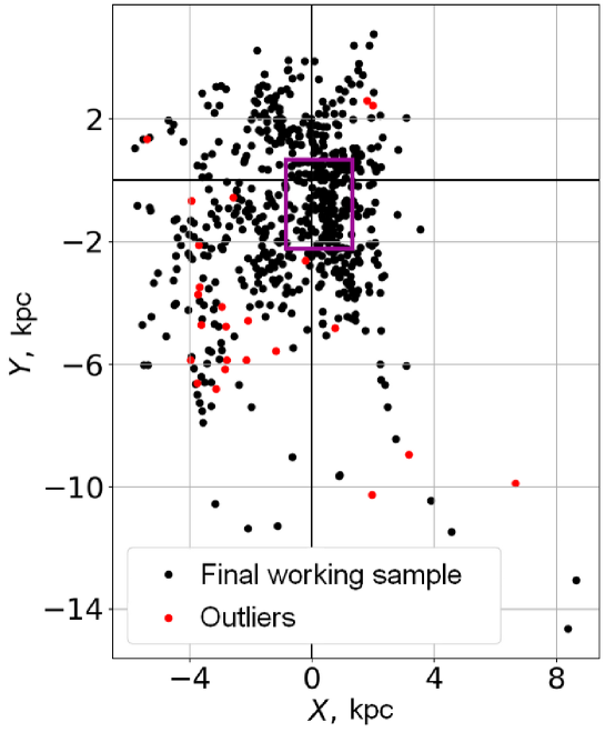
Figure 1: Objects of the final working sample and outliers projected onto the $XY$ plane. The purple rectangle marks the boundary of the local sample (see text). $X$-axis is directed towards the Galactic center, $Y$-axis is towards the rotation of the Galaxy. The Sun is placed at $X=0$ kpc, $Y=0$ kpc.

We also identified a local sample, which is part of the working sample representing the largest neighborhood of the Sun with the property of relative completeness of the identification of objects of this type (classical Cepheids). Assuming a homogeneous distribution of objects projected onto the $XY$-plane (the Galactic plane) in a vicinity of the Sun, the number of objects projected onto a section of the $XY$-plane should be proportional to the area of this section. Usually, a set of concentric rings is used to select a local, close to complete, subsample, but the working sample has an asymmetry with respect to the origin of coordinates on the $XY$ plane. For this reason, it was decided to use a set of rectangular frames with borders homothetic to the rectangular border of the working sample: the lengths of each side of the frame vary according to a given scale factor, and the ratio of distances from the origin to the edges of the frames remain constant (Fig. 2, left panel). In the case of a small frame width, the area of the frame will be proportional to the outer perimeter, so for a complete sample, the number of objects in the frame should increase linearly with the size of the frame (scale factor). On the right panel of Fig. 2 the linear growth is observed within the first three bins (frames), which are marked in red; objects within these frames were taken as a local sample. The boundaries of this sample are shown in Fig. 1 (purple rectangle). The sample size is 154. After excluding an outlier, the final local sample of 153 objects was obtained.

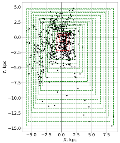
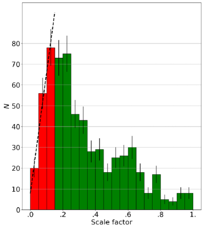
Figure 2: Left: Homothetic boundaries of rectangular frames used to construct the local sample (see text), superimposed on the distribution of objects of the working sample in projection on the $XY$ plane. Right: Histogram of the distribution of objects of the working sample in rectangular frames. The red color corresponds to the frames within which the sample (local sample) can be considered complete; the dashed straight line shows the linear growth area of the number of objects in the first three bins.

4 Results

The influence of the accepted order of the model $\zeta_{n}$ on the results can be illustrated by the example of the dependence of $z_{00}$ on $n$ for the final working sample (Fig. 3). It can be seen that for small orders the estimates of $z_{00}$ strongly depend on $n$, while for larger orders the estimates vary insignificantly.

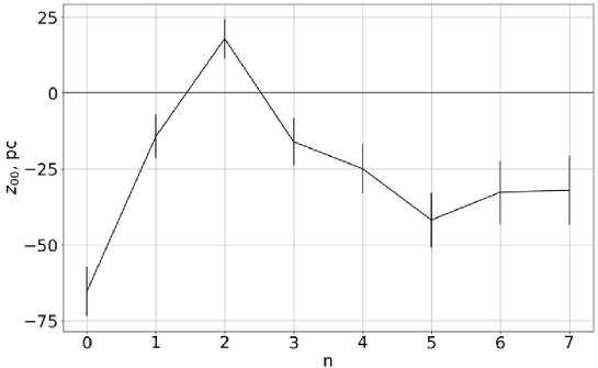
Figure 3: Dependence of $z_{00}$ (${=}-z_{\sun}$) on the model order $n$ for the final working sample. Vertical bars show the uncertainties of estimates.

The optimal order of the model $\zeta_{n}$ for the final working sample turned out to be $n_{\text{o}}=4$. Estimates of model parameters are presented in Table 1, significant estimates are given in bold. For the local and final local samples, $n_{\text{o}}$ is $0$. Final results for $z_{\sun}$ and $\sigma_{\rho}$ without and with the correction of distance scale (5) for the final working and final local samples are listed in Table 2. Comparison with Figure 3 shows that the choice of an underestimated order ($n<n_{\text{o}}$) of the model can lead to an obviously incorrect estimate of $z_{\sun}$ (here at $n=0$, 2).

Table 1: Parameter estimates for the model $\zeta_{n}$ of the average surface of the Galactic disk of optimal order $n_{\text{o}}=4$ obtained for the final working sample of classical Cepheids. Estimates that differ from zero at a significance level of at least $2\sigma$ are highlighted in bold. The standard deviation ${\sigma_{\rho}}$ is given in kiloparsecs, while values of $z_{ij}$ are in units of $\text{kpc}^{1-i-j}$

Parameter	Estimation	$\sigma_{z_{i}}/|z_{i}|$	Parameter	Estimation	$\sigma_{z_{i}}/|z_{i}|$
$\sigma_{\rho}$	$0.1187\pm 0.0033$	$0.03$	$z_{21}$	$0.00289\pm 0.00094$	$0.33$
$z_{00}$	$-0.0243\pm 0.0079$	$0.33$	$z_{12}$	$0.00288\pm 0.00055$	$0.19$
$z_{10}$	$-0.0320\pm 0.0061$	$0.19$	$z_{03}$	$0.00180\pm 0.00028$	$0.16$
$z_{01}$	$-0.0131\pm 0.0040$	$0.31$	$z_{40}$	$-0.00012\pm 0.00012$	$1.00$
$z_{20}$	$0.0055\pm 0.0025$	$0.45$	$z_{31}$	$0.00013\pm 0.00014$	$1.08$
$z_{11}$	$0.0008\pm 0.0018$	$2.25$	$z_{22}$	$0.00022\pm 0.00010$	$0.45$
$z_{02}$	$-0.0007\pm 0.0010$	$1.43$	$z_{13}$	$0.000185\pm 0.000048$	$0.26$
$z_{30}$	$0.00203\pm 0.00087$	$0.43$	$z_{04}$	$0.000099\pm 0.000020$	$0.20$

Table 2: Final estimates of $z_{\sun}$ and $\sigma_{\rho}$ for the optimal models $\zeta_{n_{\text{o}}}(X,Y)$ obtained for two samples of Cepheids. The estimates are given in the original catalog distance scale and in the scale adjusted for calibration $d_{\text{LMC}}=18.49\pm 0.09\,\text{mag}$ (see text)

Sample	Original distance scale	Corrected distance scale
Final working sample	$z_{\sun}=24.3\pm 7.9\ \text{pc}$	$z_{\sun}=27.1\pm 8.8\big{|}_{\text{stat.}}\>^{+1.3}{}_{-1.2}\big{|}_{\text{cal.}}\>\text{pc}$
($N=615$, $n_{\text{o}}=4$)	$\sigma_{\rho}=118.7\pm 3.3\ \text{pc}$	$\sigma_{\rho}=132.0\pm 3.7\big{|}_{\text{stat}}\>^{+6.3}{}_{-5.9}\big{|}_{\text{cal.}}\>\text{pc}$
Final local sample	$z_{\sun}=25.2\pm 5.5\ \text{pc}$	$z_{\sun}=28.1\pm 6.1\big{|}_{\text{stat.}}\>\pm 1.3\big{|}_{\text{cal.}}\>\text{pc}$
($N=153$, $n_{\text{o}}=0$)	$\sigma_{\rho}=68.5\pm 3.9\ \text{pc}$	$\sigma_{\rho}=76.5\pm 4.4\big{|}_{\text{stat.}}\>^{+3.6}{}_{-3.4}\big{|}_{\text{cal.}}\>\text{pc}$

The model surface $\zeta_{4}(X,Y)$ for the final working sample is shown in Figure 4. Here the level

$${\zeta_{4}}(X,Y)=z_{00}$$ (6)

is represented by a black line. This line is the intersection of the model of the average surface of the disk with the nominal plane of the Galaxy $XY$. Line (6) corresponds to the line-of-nodes in simple models. Figure 4 shows that in reality the line (6), skirting the areas of local extrema, is quite curved. By analogy with the line-of-nodes, the curve $\zeta_{n_{\text{o}}}(X,Y)=z_{00}$ can be called a “curve-of-nodes”. Of course, the constructed model $\zeta_{4}(X,Y)$ is real only for the area of the disk that is covered by the data used. Boundaries of areas within which the mean error of the model is $\sigma_{\zeta_{4}}(X,Y)\leq\frac{1}{6}\sigma_{\rho}=20\,\text{pc}$, ${\leq}\frac{1}{4}\sigma_{\rho}=40\,\text{pc}$ and ${\leq}\frac{1}{2}\sigma_{\rho}=59\,\text{pc}$ shown in Figure 4 by dotted, dashed and dashed–dotted lines, respectively, give an idea of the applicability of the model $\zeta_{4}$ depending on the specified level of its uncertainty. Here $\sigma_{\zeta_{4}}(X,Y)$ was calculated using the formula (4), and $\sigma_{\rho}=119$ pc (see Table 1).

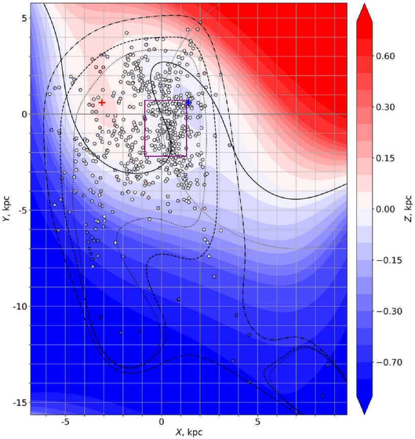
Figure 4: A map of the model $\zeta_{4}$ of the average disk surface of optimal order, constructed from the objects of the final working sample. The color shows the value of the function $\zeta_{4}(X,Y)$. The objects are shown as colored circles with color representing the $Z$-coordinate. The black line represents the $z_{00}$-level, the red and blue crosses depict the local extrema (maximum and minimum, respectively), the purple rectangle shows the boundary of the local sample, the grey line denotes the solar circle $R=R_{0}=8$ kpc. The dotted, dashed and dashed–dotted lines are the boundaries of the applicable areas of the model $\sigma_{\zeta_{4}}$, within which the mean error of the model is $\sigma_{\zeta_{4}}(X,Y)\leq\frac{1}{6}\sigma_{\rho}=20\,\text{pc}$, ${\leq}\frac{1}{4}\sigma_{\rho}=40\,\text{pc}$ and ${\leq}\frac{1}{2}\sigma_{\rho}=59\,\text{pc}$, respectively.

An alternative representation of the resulting model is given in Figure 5, which shows the extremum and boundary lines of the model surface $\zeta_{4}(X,Y)$ in projections on the planes $XZ$ and $YZ$ in comparison with the Cepheids of the final working sample. The extremum lines (there may be several of them for each projection) are dependencies of $Z$-coordinates of points of local extremes of the surface $\zeta_{4}(X,Y)$ with fixed $X$—$\zeta_{\text{max}}(X,\mathbf{Y})$, $\zeta_{\text{min}}(X,\mathbf{Y})$ (Figure 5, top panel) or with fixed $Y$—$\zeta_{\text{max}}(\mathbf{X},Y)$, $\zeta_{\text{min}}(\mathbf{X},Y)$ (bottom panel). The boundary lines show the values of $\zeta_{4}(X,Y)$ at the boundaries of the final working sample: $\zeta_{4}(X,Y_{\text{min}})$ and $\zeta_{4}(X,Y_{\text{max}})$ (top panel), and $\zeta_{4}(X_{\text{min}},Y)$ and $\zeta_{4}(X_{\text{max}},Y)$ (bottom panel), where $X_{\text{min}}=-5.8$ kpc, $X_{\text{max}}=8.6$ kpc, $Y_{\text{min}}=-14.6$ kpc, $Y_{\text{max}}=4.8$ kpc. Figure 5 affirms that the extremum lines mainly fall on the areas covered by the data, and the boundary lines indicate edge approximation effects in the area $X\gtrsim 4$ kpc, $Y\gtrsim 0$ kpc.

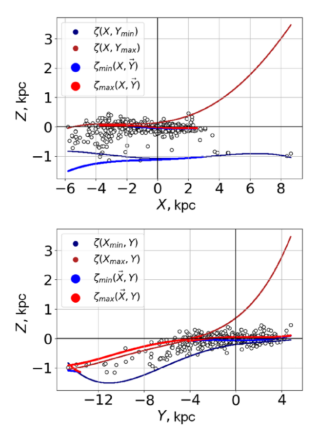
Figure 5: Extremum lines (thicker lines of lighter color) and boundary lines of the model surface $\zeta_{4}(X,Y)$ in comparison with Cepheids of the final working sample in the projection on the plane $XZ$ (top panel) and $YZ$ (bottom panel); see text. Local maxima and lines of the largest values of $\zeta_{4}$ at the sample boundaries are shown in red, while local minima and lines of the smallest boundary values are shown in blue.

The well-known general shape of the Galactic disk warp is clearly visible in Figure 4—in the first and second quadrants, the model surface as a whole rises above the $XY$ plane; in the third and fourth quadrants, the surface decreases below this plane. In the area near $X\approx-3$ kpc, $Y\approx-6$ kpc, the decrease in the average surface is observed for almost all objects.

However, in addition, we found two extrema in the first and second quadrants that do not fit into simple warp models. The sections of the model with planes parallel to the $XZ$ and $YZ$ planes and passing through the points of extrema are shown in Figure 6. The significance $S$ of the extrema was estimated by the formula

$$S_{\zeta_{4}}(X,Y)=\frac{\zeta_{4}(X,Y)-z_{00}}{\sigma_{\zeta_{4}}(X,Y)}\,.$$ (7)

Table 3 shows the parameters of local extrema. The given values of $S$ show that the local minimum and maximum are significant at the level of at least $2\sigma$ and $5\sigma$, respectively.

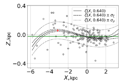
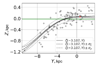
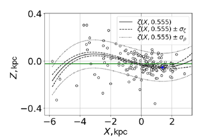
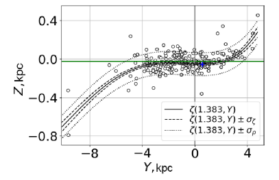
Figure 6: Sections of the model $\zeta_{4}(X,Y)$ of the middle surface of the disk passing through the local maximum (upper panels) and minimum (lower panels). Each panel shows the confidence area for the model values $\zeta_{4}(X,Y)$ ($\pm 1\sigma_{\zeta}$) and the area of object deviations from the model $\pm 1\sigma_{\rho}$, as well as projections of the position of objects located in the $\pm 1\,\text{kpc}$ band from the cut line. The green line indicates the position of the plane $Z=z_{00}$.

Table 3: Parameters of local extrema of the optimal model $\zeta_{4}(X,Y)$ constructed for the final working sample: The Cartesian heliocentric coordinates $X,Y$ of the extremum, the value of $\zeta_{4}(X,Y)$ at the extremum point and the significance level $S_{\zeta_{4}}(X,Y)$ of the extremum (the number of $\sigma$)

Extremum	$X$ (kpc)	$Y$ (kpc)	$\zeta_{4}(X,Y)$ (pc)	$S_{\zeta_{4}}(X,Y)$
Local maximum	$-3.1$	$0.6$	$58.4\pm 15.0$	$5.43$
Local minimum	$1.4$	$0.6$	$-55.0\pm 11.0$	$-2.81$

In Figure 6 the slope of the model surface $\zeta_{4}(X,Y)$ to the nominal plane of the Galaxy $XY$ is visible. Having calculated the distance $\rho_{\sun}$ from the Sun to the surface $\zeta_{4}(X,Y)$ along the normal to the latter, we obtained an estimate of the angle of inclination of the local average surface of the Galactic disk to the plane $XY$ of the galactic coordinate system

$$\gamma=\arccos\left(\frac{\rho_{\sun}}{z_{\sun}}\right)=1\fdg 79^{+0\fdg 34}_{-0\fdg 33}.$$ (8)

The $1\sigma$-uncertainty of the angle $\gamma$ indicated here was found by the Monte Carlo method based on the results of processing 50 mock data catalogs.

According to Pearson’s chi-square test, the probability density function $f(\rho)$ (2) does not fit data well (see Fig. 7, left panel)—the probability of accepting the null hypothesis that the observed distribution has a probability density of the form (2) is less than $1\%$. This means the other functions $f(\rho)$ or combinations of them should be considered in the future. However, for the final local sample the chi-square test gives a probability of acceptance of the hypothesis (2) of about $30\%$ (see Fig. 7, right panel), i.e., the Gaussian distribution as a model for $f(\rho)$ should not be excluded from consideration.

  

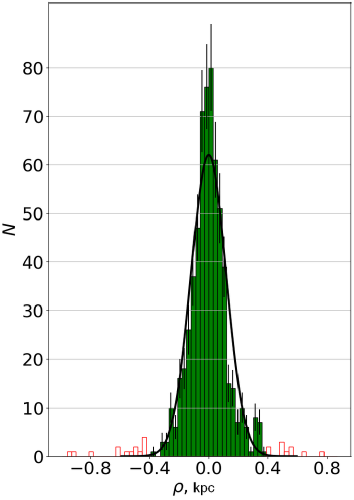
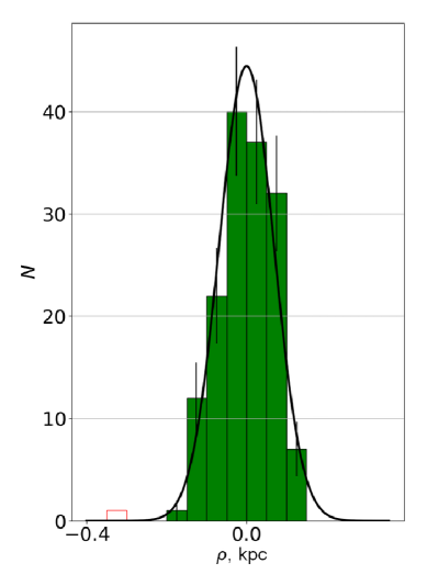
Figure 7: Observed (green columns) and model (black line) distributions of object deviations $\rho$ along the normal to the model average surface for the working sample (left panel, for $n_{\text{o}}=4$ and the model parameters given in Table 1) and local sample (right panel, for $n_{\text{o}}=1$ and the parameters given in Table 2). Outliers are shown in red.

Since in this paper we used a catalog (Mel’nik et al. 2015) based on observations in infrared bands ($I_{\text{C}}$ and $K$; see Dambis et al. 2015), this allows us to expect a low selection effect due to the absorption of light by dust in the Galactic disk. In particular, there should be no significant differential selection in the vertical direction, i.e., statistical sample bias to the north of the disk. Indeed, due to the position of the Sun above the average surface of the disk, a ray of light from an object located south of the average surface of the disk passes through a larger thickness of the disk and experiences greater light absorption. Indeed, due to the position of the Sun above the average surface of the disk, a ray of light from an object located south of the average surface of the disk passes through a larger thickness of the disk and experiences greater light absorption compared to a northern object at the same distance from the average surface. Therefore, in principle, one would expect a sharper truncation of the observed distribution of deviations $\rho$ from the model from the negative $\rho$ side compared to the positive ones, i.e., greater detection of northern objects compared to southern ones. Asymmetry of this type in the distribution of deviations $\rho$ does not really manifest itself in a noticeable way (fig. 7). In reality, for the working sample, instead of a sharper truncation on negative $\rho$, rather on the contrary, there is some deficit on $\rho\sim+0.2$ kpc (fig. 7, left panel). The standard deviation calculated for objects with $\rho>0$ pc for any sample does not significantly exceed the standard deviation found for objects with $\rho<0$ kpc (see Table 4). These results support of the insignificance of north–south selection.

Table 4: Standard deviations of Cepheids across the disk, calculated for objects of the considered samples with only positive deviations $\rho$ from the model, $\sigma_{\rho}^{+}$, and with only negative ones, $\sigma_{\rho}^{-}$

Sample	$\sigma_{\rho}^{+}$ (kpc)	$\sigma_{\rho}^{-}$ (kpc)
Working sample	$0.1621\pm 0.0045$	$0.1641\pm 0.0046$
Final working sample	$0.1277\pm 0.0053$	$0.1162\pm 0.0048$
Local sample	$0.0765\pm 0.0043$	$0.0894\pm 0.0046$
Final local sample	$0.0757\pm 0.0043$	$0.0792\pm 0.0043$

Note that the increase in the selection effect with distance from the Sun in the sense of incomplete sampling (Fig. 2, right panel) does not in itself lead to bias, i.e., to systematic errors in the position of the average (model) surface of the disk and in estimation of the dispersion of objects relative to this surface. Classical Cepheids belong to population I and, being quite young objects—${\sim}10^{7}$–$10^{8}$ years (see, e.g., Veselova & Nikiforov 2020)— represent a thin disk of the Galaxy. Moreover, the vertical deviation of the subsystem of classical Cepheids $\sigma_{\rho}{\sim}130$ pc (this work) is significantly smaller than the average vertical scale $h_{z}=300\pm 50$ pc of the thin disk as a whole (Bland-Hawthorn & Gerhard 2016). This makes classical Cepheids a good tracer of the thin disk of the Galaxy: even in areas where there are few of them, they still represent the position of the disk with a relatively small spread. In such areas the mathematical expectation of the average $Z$-coordinate of the Cepheids, $\overline{Z}$, remains equal to the true $Z$-coordinate of the average surface of the disk, only the mean error of $\overline{Z}$ estimate increases, i.e., in the case of our method, the mean error of the model $\sigma_{\zeta_{4}}$ increases (isolines of $\sigma_{\zeta_{4}}(X,Y)$ are shown on Figure 4).

On the other hand, Cepheids, concentrating towards spiral arms (see, e.g., Veselova & Nikiforov 2020), like other tracers of the spiral structure of the Galaxy, often have not a uniform, but a “patchy” distribution along the spiral arms (for example, Efremov 2011, fig. 1; Nikiforov & Veselova 2018, fig. 13; Reid et al. 2019, fig. 2; Veselova & Nikiforov 2020, fig. 5). This, as well as the growth of incomplete detection of objects and a decrease in the density of the disk to the periphery, leads to the fact that at large distances from the Sun, gaps appear in the distribution of Cepheids, for example at $(X,Y)\sim(0,-7)$ kpc (Figure 4). Of course, in the areas of such gaps, the constructed model should be treated only as a smooth interpolation of the average trend between the areas represented by the data. However, when imposing a stricter restriction on the mean error of the model, e.g., $\sigma_{\zeta_{4}}(X,Y)\leq\frac{1}{6}\sigma_{\rho}=20\,\text{pc}$, the internal area of applicability of the model does not include most of these lacunae (see Figure 4). The relatively high accuracy of the model for the area in the lower right corner of Figure 4 is, of course, only formal, due to the fact that any sufficiently flexible model must pass through a few Cepheids in this area, located at some distance from the bulk of the sample objects. On the other hand, these and other Cepheids at large negative $Y$ are in the general trend of a well-known decrease in the average surface of the disk in this area. So, in the region  $Y<-10$ kpc, all Cepheids of the working sample are in the range $-1.2\leq Z\leq-0.8$ kpc (Figure 5, bottom panel), which agrees well with the disk level in this area according to other data—e.g., $-2\leq Z\leq 1$ kpc (Skowron et al. 2019b, from Cepheids), $\overline{Z}=-1.22$ kpc (Romero-Gómez et al. 2019, from red giant branch (RGB) stars), $-1\leq Z\leq-0.5$ kpc (Lemasle et al. 2022, from Cepheids). The vertical dispersion of objects at large negative $Y$ is consistent with that for the rest of the working sample (Figure 5, bottom panel). At the same time, the use of the entire working sample, despite the gaps, does not create any fictitious ripples in the model of the average surface of the disk in the area $Y<-6$ kpc (Figure 4, 6). Thus, there was no reason to discard Cepheids at large negative $Y$. In addition, it was important to keep in the sample objects representing the decline of the disk surface in the III and IV quadrants in order to test the capabilities of the general model (1) within the framework of the proposed method to describe this well-known feature together with other possible details of the disk surface (as it turned out, local extremes). Note that the value of the decrease in the disk level of $\Delta Z{\sim}1$ kpc relative to the plane $Z=z_{00}$ is much larger than the standard deviation for Cepheids ($\sigma_{\rho}\sim 130$ pc), i.e., the downward trend is detected confidently, despite the incompleteness of the sample in this area.

We tested the algorithm used here for choosing the optimal order of the $\zeta_{n}$ model by the Monte Carlo method. As a model of the disk surface, the constructed model $\zeta_{4}$ was adopted (Table 1) and 100 mock catalogs were generated with object deviations from $\zeta_{4}(X,Y)$ along the normal to this surface, distributed according to the law (2) with the value of $\sigma_{\rho}$ indicated in Table 1. The results are shown in Figure 8. They show that in most cases the order of the initial model is restored exactly, and the probability that the order of the model will be underestimated is less than 1%. These results suggest that, acting according to this algorithm, it is possible to obtain a model that does not fully reflect some details of the real disk structure, but it is unlikely to build an excessively complex model with fictitious details.

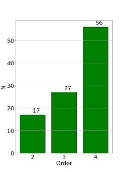
Figure 8: Distribution of optimal order values for 100 mock samples (see text).

Table 5: Same as in Table 1, but for the odd subsample of the final working sample (see text). $n_{\text{o}}=4$

Parameter	Estimation	$\sigma_{z_{i}}/|z_{i}|$	Parameter	Estimation	$\sigma_{z_{i}}/|z_{i}|$
$\sigma_{z}$	$0.1218\pm 0.0050$	$0.04$	$z_{21}$	$0.0017\pm 0.0013$	$0.76$
$z_{00}$	$-0.026\pm 0.011$	$0.42$	$z_{12}$	$0.00214\pm 0.00080$	$0.37$
$z_{10}$	$-0.0321\pm 0.0093$	$0.29$	$z_{03}$	$0.00145\pm 0.00040$	$0.28$
$z_{01}$	$-0.0077\pm 0.0061$	$0.79$	$z_{40}$	$0.00025\pm 0.00022$	$0.88$
$z_{20}$	$0.0074\pm 0.0039$	$0.53$	$z_{31}$	$0.00026\pm 0.00021$	$0.81$
$z_{11}$	$-0.0002\pm 0.0026$	$13.00$	$z_{22}$	$-0.00008\pm 0.00018$	$2.25$
$z_{02}$	$-0.0013\pm 0.0014$	$1.08$	$z_{13}$	$0.000133\pm 0.000065$	$0.49$
$z_{30}$	$0.0038\pm 0.0015$	$0.39$	$z_{04}$	$0.000092\pm 0.000029$	$0.32$

To check the stability of the results, we divided the final working sample (hereinafter, for short, “full sample”) into two parts: one part included objects with odd numbers in the sample list (we will call it the odd subsample), and the other objects with even numbers (even subsample). This separation is actually random. On the other hand, it keeps the relative population of data of different longitude intervals approximately the same for both subsamples and for the full sample, since in the catalog Mel’nik et al. (2015) objects are ordered by their names, i.e., mainly by the names of constellations. The latter is important if we want to check the reproducibility of the detected details on the relief of the disk surface. The calculations were repeated for each of the two independent subsamples. The results are presented in Tables 5–7 and in Figure 9. The optimal orders of the model $\zeta_{n}$ for both subsamples turned out to be the same and equal to $n_{\text{o}}$ for the full sample: $n_{\text{o}}=4$. The parameters of the model $\zeta_{4}$ for even and odd subsamples and for the full sample within the error limits are consistent with each other (cf. Tables 1, 5, 6). At the same time, all significant parameters obtained from subsamples are also significant for the full sample. The characteristics of the local extremes for the odd subsample turned out to be similar to the characteristics for the full sample (cf. Tables 3, 7). For the even subsample, the model $\zeta_{4}(X,Y)$ does not formally have local extremes, but it has areas of depression and elevation (Figure 9, right panel), in position and amplitude close to those for models obtained from the full sample and odd subsample (Figure 4; Figure 9, left panel). The curves-of-nodes also turned out to be similar for all three samples in the area of applicability of the model (Figures 4, 9). Thus, the topology of the resulting model as a whole is preserved even when the sample is divided. At the same time, the drop in the significance of the details of the model surface $\zeta_{4}(X,Y)$ for subsamples shows that dividing the sample into a larger number of parts is hardly meaningful.

Table 6: Same as in Table 1, but for the even subsample of the final working sample (see text). $n_{\text{o}}=4$

Parameter	Estimation	$\sigma_{z_{i}}/|z_{i}|$	Parameter	Estimation	$\sigma_{z_{i}}/|z_{i}|$
$\sigma_{z}$	$0.1227\pm 0.0050$	$0.04$	$z_{21}$	$0.0037\pm 0.0015$	$0.41$
$z_{00}$	$-0.028\pm 0.011$	$0.39$	$z_{12}$	$0.00249\pm 0.00086$	$0.35$
$z_{10}$	$-0.0279\pm 0.0097$	$0.35$	$z_{03}$	$0.00210\pm 0.00044$	$0.21$
$z_{01}$	$-0.0167\pm 0.0060$	$0.36$	$z_{40}$	$-0.00030\pm 0.00020$	$0.67$
$z_{20}$	$0.0046\pm 0.0036$	$0.78$	$z_{31}$	$0.00010\pm 0.00020$	$2.00$
$z_{11}$	$0.0011\pm 0.0028$	$2.55$	$z_{22}$	$0.00035\pm 0.00016$	$0.46$
$z_{02}$	$0.0011\pm 0.0016$	$1.45$	$z_{13}$	$0.000125\pm 0.000088$	$0.70$
$z_{30}$	$0.0008\pm 0.0014$	$1.75$	$z_{04}$	$0.000097\pm 0.000033$	$0.34$

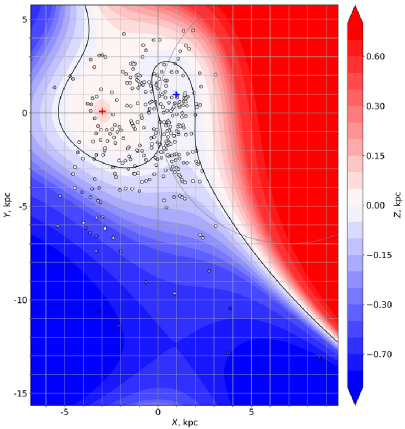
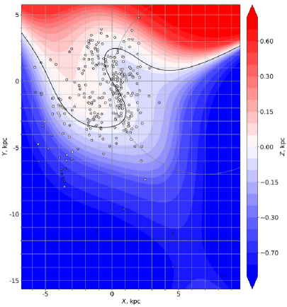
Figure 9: Maps of the models $\zeta_{4}$ of the average disk surface of optimal order, constructed from the objects of independent odd (left panel) and even (right panel) subsamples of the final working sample (see text). The notation is the same as in Figure 4.

Table 7: Same as in Table 3, but for the odd subsample of the final working sample (see text)

Extremum	$X$ (kpc)	$Y$ (kpc)	$\zeta_{4}(X,Y)$ (pc)	$S_{\zeta_{4}}(X,Y)$
Local maximum	$-3.0$	$0.1$	$53.0\pm 20$	$4.01$
Local minimum	$1.0$	$1.0$	$-50.4\pm 15$	$-1.59$

5 Discussion

Consistency of local solar offset estimate $z_{\sun}=28.1\pm 6.1\big{|}_{\text{stat}}\>^{+1.3}{}_{-1.3}\big{|}_{\text{cal}}\>\text{pc}$ and global estimate $z_{\sun}=27.1\pm 8.8\big{|}_{\text{stat}}\>^{+1.3}{}_{-1.2}\big{|}_{\text{cal}}\>\text{pc}$ (Table 2) also implies that the proposed algorithm is valid and the model order is correct—when optimizing the order of the model, the value of the solar offset does not depend systematically on whether a large or small neighborhood of the Sun is considered. Our estimates also agree with the best estimate of the solar offset $z_{\sun}=25\pm 5\,\text{pc}$ (Bland-Hawthorn & Gerhard 2016) and local estimates specifically for classical Cepheids (see below).

However, the estimate of $\sigma_{\rho}=68.5\pm 3.9$ pc obtained for the final local sample is inconsistent with the estimate of $\sigma_{\rho}=118.7\pm 3.3$ pc for the final working sample (in original distance scale, see Table 2). Since the estimates were obtained by optimizing the order of the model $\zeta_{n}$, this mismatch should mainly be a consequence of a combination of the flaring and random errors in distances. Indeed, the observed deviation of objects relative to the model $\zeta_{n_{\text{o}}}$ is due to two factors: the natural (true, cosmic) dispersion of objects relative to the average surface of the Galactic disk and the measuring dispersion—the deviation of the observed positions of objects from their true positions due to random errors in distance moduli. The latter means that more distant objects have larger distance errors. On the other hand, the natural dispersion can grow to the periphery (the disk flaring). Indeed, at $X<0$ kpc, the apparent spread of objects relative to the model increases somewhat (Figure 6, left panels). In order to separate the contributions of these two effects, a more complex version of the present method is required with direct consideration of random errors in distances. This will allow you to get more reliable results about flaring itself.

Note that the contribution of the measuring dispersion to the observed dispersion $\sigma_{\rho}$ in this case is very small, as shown by the following approximate estimates. For photometric distances, their standard deviation due to measuring dispersion is $\sigma_{r}=\frac{\ln 10}{5}\,\sigma_{d}\,r$, where $\sigma_{d}$ is the standard uncertainty of distance moduli. In the case of local sample, the main contribution of distance errors to the observed vertical standard deviation $\sigma_{Z}$ (close to $\sigma_{\rho}$) occurs due to objects at high latitudes $b$. Then the assumption that the standard $\sigma_{r}$ for all objects of the sample completely passes into vertical standard deviation gives an upper estimate for the contribution of the measuring dispersion to $\sigma_{Z}$: $\sigma_{Z,\text{mes}}<\sigma_{r}$. For the distance $r=1\sigma_{\rho}=76.5$ pc (see Table 2) and $\sigma_{d}=0.14^{m}$ (Veselova & Nikiforov 2020), this results in $\sigma_{Z,\text{mes}}<4.9$ pc and the natural dispersion $\sigma_{Z,0}=\sqrt{\sigma_{Z}^{2}-\sigma_{Z,\text{mes}}^{2}}>76.3$ pc, i.e., the correction is no more than $-0.2\%$.

In the case of a working sample, most of the objects are located at small $|b|$: for characteristic distances $r=3$–$6$ pc (see Fig. 1) and $Z=1\sigma_{\rho}=132$ pc (Table 2) $|b|=1\fdg 3$–$2\fdg 5$. For sample objects, the contribution of the measuring dispersion is $\sigma_{Z,\text{mes}}=\sigma_{r}\sin|b|$, $\tan b=Z/(r\cos b)$, then for small $|b|$ $b\approx Z/r$, $\sigma_{Z,\text{mes}}\approx\sigma_{r}|b|=\frac{\ln 10}{5}\,\sigma_{d}\,|Z|$. Then for $Z=1\sigma_{\rho}=132$ pc it turns out: $\sigma_{Z,\text{mes}}\approx 8.5$ pc, $\sigma_{Z,0}\approx 131.7$ pc, i.e., correction $-0.2\%$. Thus, in both cases, the contribution of random distance uncertainty to the observed vertical dispersion is negligible.

From classical Cepheids on $r<2$ kpc Majaess et al. (2009) obtained $z_{\sun}=26\pm 3$ pc and the scale height of ${\leq}75\pm 10$ pc which are consistent with our estimates (Table 2). Estimates of $z_{\sun}=(23$–$24)\pm 2\;\text{pc}$ and $\sigma_{\rho}=76.4\pm 1.8\;\text{pc}$ were found by Bobylev & Bajkova (2016a) for classical Cepheids according to the same version of the Berdnikov et al.’s catalog as in this work. Bobylev & Bajkova (2016a) considered the cylindrical region $r\leq 4$ pc. As they used the original calibration of the catalog we can compare these estimates with ours in the same calibration (Table 2). There is consistency with our estimates of the solar offset for both final local and final working samples. However, the vertical scale estimates are consistent only in the case of final local sample. Exactly the same situation is for Cepheids-based estimates in Skowron et al. (2019a). The authors considered data on 2431 Cepheids, and the most part of the data was obtained by the OGLE-IV project. Skowron et al. obtained an estimate of the disk scale height of $73.5\pm 3.2$ pc, so our estimate for the final local sample does not contradict this value. All this also points out the importance of taking into account the warp of the Galactic average disk surface in order to have the ability of proper consideration of all the data available. Otherwise, only local regions can be considered.

In addition, the fact that the estimates of $z_{\odot}$ differ, as noted in Introduction, also suggests that the a priori assumption about the flat model of the Galactic disk should be limited. Indeed, according to our results such assumption might be made only for specific regions like the local one, i.e., close enough to the Sun. Moreover, it can be noticed that the value of $z_{\sun}$ is less dependent on the Galactic disk warping than the value of $\sigma_{\rho}$. Based on what has been said, we can conclude that any a priori assumption about the Galactic disk warping must be carefully studied especially when the vertical scale parameter is estimated.

The detected local extrema of the average surface of the disk may be manifestations of bending waves caused by interaction with the Sagittarius dwarf galaxy, in the form of local structures elongated in the azimuthal direction (Gómez et al. 2013, fig. 5; Laporte et al. 2019; Poggio et al. 2021, fig. 2), or by interaction with the Large Magellanic Cloud (Thulasidharan et al. 2022 and references therein).

The method used after testing on classical Cepheids can now be applied to other data (in particular, to Gaia data) and/or in other assumptions about the distribution function $f(\rho)$. The Gaia DR2 catalog was used in recent work by Ablimit et al. (2020) to obtain data on classical Cepheids. Despite the fact the direct study of the Galactic disk warping was not conducted in the work of these authors, according to the pictures plotted in the work on these data, the disk warping is clearly revealed. Unfortunately, the use of the current version of our method with these data as is will lead to significant biases mainly because of the dependence of distance uncertainty on distance, which will be significant due to the need to consider the large neighborhood of the Sun.

Taking into account the uncertainty of distances may also solve the problem of establishing the form of the vertical distribution law $f(\rho)$. Note that the analysis of the 2D distribution does not allow us to draw a definite conclusion about the functional form of this law (Mosenkov et al. 2021).

In the future, we plan to apply the proposed method in the variant of accounting for distance uncertainties to new databases.