Role of chemical potential at kinetic freeze-out using Tsallis non-extensive statistics in proton-proton collisions at the Large Hadron Collider

Abstract

The charged-particle transverse momentum spectra ($p_{\rm T}$-spectra) measured by ALICE collaboration for $pp$ collisions at $\sqrt{s}=$ 7 and 13 TeV have been studied using a thermodynamically consistent form of Tsallis non-extensive statistics. The Tsallis distribution function is fitted to the $p_{\rm T}$-spectra and the results are analyzed as a function of final state charged-particle multiplicity for various light flavor and strange particles, such as $\pi^{\pm},K^{\pm},p+\bar{p},\phi,\Lambda+\bar{\Lambda},\Xi+\bar{\Xi},\Omega+\bar{\Omega}$. At LHC energies, particles and antiparticles are produced in equal numbers. However, there are various processes that contribute to the asymmetry between hadrons and anti-hadrons at kinetic freeze-out, which could contribute to make the chemical potential finite. This article emphasizes the importance of the chemical potential of the system produced in $pp$ collisions at the LHC energies using the Tsallis distribution function.

I Introduction

It has been the ambitious force of research in high-energy physics to use particle colliders like the Relativistic Heavy Ion Collider (RHIC) at Brookhaven National Laboratory (BNL) and the Large Hadron Collider (LHC) at CERN (European Council for Nuclear Research), which fulfill the appetite for understanding the matter formed during ultra-relativistic collisions. The primary objective of these experiments is to create extreme conditions of high temperature and/or energy densities through compression or heating in high-energy nuclear collisions Gyulassy:2004zy ; Braun-Munzinger:2007edi ; Jacak:2012dx , where a system of deconfined quarks and gluons can be formed. These extreme conditions lead to the asymptotic freedom of the QCD system, where the quarks and gluons are no longer confined inside the nucleon Itoh:1970uw ; Collins:1974ky ; Cabibbo:1975ig ; Chapline:1976gy . Afterwards, the produced system undergoes expansion through cooling of the systems where the quarks and gluons are combined to form hadrons. In this course of action, the inelastic collisions cease at the chemical freeze-out boundary where the stable particle yields get fixed at chemical freeze-out temperature ($T_{\rm ch}$). Finally, at the kinetic freeze-out boundary the elastic collisions among the final state particles no longer exist and a stream of particles gets detected in our detectors. This enables us to get the kinetic freeze-out temperature ($T_{\rm th}$) of the system from the transverse momentum spectra of the identified particles. The chemical freeze-out stage is well understood and is strongly supported by experimental results Andronic:2017pug . Furthermore, the results are in agreement with a Lattice Quantum Chromodynamics (LQCD) model based on first principles and a well-established hydrodynamic technique Sollfrank:1990qz . Similarly, the kinetic freeze-out stage has also been explored by several phenomenological works, where information about the system is extracted by fitting different fitting functions to the transverse momentum spectra of the final state particles.

Over the past several years, numerical studies of lattice QCD have been successful at high temperatures and with zero chemical potential. However, studying the phase structure of QCD at non-zero chemical potential is one of the most exciting problems in contemporary physics Allton:2002zi ; Allton:2003vx ; Gavai:2003mf ; Allton:2005gk ; Bazavov:2017dus . It is noteworthy that on the theoretical side, the color superconducting and superfluid phases have been conjectured at high baryon densities Book . Therefore, it is necessary to investigate the QCD phase transition utilizing lattice gauge theory simulations at the non-zero chemical potential. As discussed in Ref.  Andronic:2017pug , a consequence of the vanishing baryon-chemical potential leads to the vanishing of strangeness chemical potential $\mu_{s}$, which implies that the strange quantum number is no longer relevant for particle production. The yield of strange and multi-strange mesons and baryons in the fireball is solely determined by their mass, $m$, spin degeneracy, $g$, and the temperature, $T$. At the LHC energies near chemical freeze-out, the baryochemical potential is expected to be zero due to both particles and antiparticles being produced in equal numbers. However, assuming the same case at the kinetic freeze-out temperature is not entirely trivial. Thus, there can be a finite total chemical potential at the kinetic freeze-out stage, and its implications cannot be ignored. Specifically, this study considers the implications of chemical potentials at kinetic freeze-out. It is worth noting that like heavy-ion collisions, in LHC $pp$ collisions, one also observes a finite hadronic phase lifetime ALICE:2019xyr ; Sahu:2019tch ; Scaria:2022lap . This prompts us to look into the effect of chemical potential in TeV $pp$ collisions at the kinetic freeze-out using the non-extensive Tsallis distribution function which describes the identified particle spectra up to several tens of GeV/c.

As discussed earlier, the $p_{\rm T}$-spectra measured in $pp$ collisions at the LHC energies can give information about the kinetic freeze-out stage of the collision. We generally fit a Boltzmann-type distribution function to the $p_{\rm T}$-spectra to extract useful information. However, the Boltzmann distribution function can only explain the low-$p_{\rm T}$ part of the spectra. As we know, transverse momenta up to hundred of GeV have been measured in high-energy hadronic collisions. This suggests that the high-$p_{\rm T}$ regime is also very significant to understand the system formed in such collisions and cannot be ignored. Power-law type distribution functions can explain the high-$p_{\rm T}$ part of the spectra very well, which comes from the perturbative QCD. But to understand the system fully, a unique distribution function is needed, which can explain both the low- and high-$p_{\rm T}$ part of the spectra. The thermodynamically consistent Tsallis distribution function has been widely used for this purpose Abelev:2006cs ; PHENIX:2010qqf ; PHENIX:2011rvu ; CMS:2010wcx ; CMS:2010tjh ; ATLAS:2010jvh ; Aamodt:2011zj ; Abelev:2012cn ; Abelev:2012jp ; Chatrchyan:2012qb . The non-extensive parameter, $q$, in the Tsallis distribution function quantifies the degree of deviation of the system from the equilibrium state. In addition, Tsallis temperature ($T$) and volume ($V$) can also be extracted by fitting the Tsallis distribution to the transverse momentum spectra.

This article is organized as follows. In the next section II, we explicitly discuss the single-particle Tsallis distribution to fit the transverse momentum spectra of the identified hadrons and determine the temperature $T$, volume $V$, and $q$ with the details of the formulation of estimating the chemical potential from kinetic freeze-out. In section III, we discuss our results, and finally, we summarize our results and conclude in section IV.

II Formulation

The Tsallis distribution function that satisfies the thermodynamic consistency relations  Cleymans:2011in ; Cleymans:2012ya ; Azmi:2015xqa is given by,

$$E\frac{d^{3}N}{d^{3}p}=gVE\frac{1}{(2\pi)^{3}}\left[1+(q-1)\frac{E-\mu}{T}\right]^{-\frac{q}{q-1}}.$$ (1)

Here, $E$ represents particles’ energy, $V$ is the volume of the system, $g$ is the degeneracy factor, $q$ is referred to as the non-extensive parameter, $T$ is the corresponding temperature, $p$ denotes the momentum, and $\mu$ is the total chemical potential ($\mu=B\mu_{B}+S\mu_{S}+Q\mu_{Q}$). Here $B$ is the baryon number, $S$ is the strangeness quantum number and $Q$ is the electric charge. Physical interpretation of $q$ can be found in ref. Wilk:1999dr . At mid rapidity, i.e, $y=0$, Eq. 1 in terms of transverse momentum, $p_{\rm T}$, transverse mass, $m_{T}=\sqrt{p_{T}^{2}+m^{2}}$ can be rewritten as,

$$\frac{d^{2}N}{dp_{T}dy}=gV\frac{p_{T}m_{T}}{(2\pi)^{2}}\left[1+(q-1)\frac{m_{T}-\mu}{T}\right]^{-\frac{q}{q-1}}.$$ (2)

For extracting Tsallis parameters for the identified non-strange, strange, and multi-strange particles, Eq. 2 has been used. The degeneracy factor $g=2\times(2s+1)$ is taken to be 2, 2, 4, 3, 8, 4 and 8 for $\pi^{\pm},K^{\pm},p+\bar{p},\phi,\Lambda+\bar{\Lambda},\Xi+\bar{\Xi},\Omega+\bar{\Omega}$ respectively. Here, $s$ is the particle’s spin, and factor 2 is for the antiparticles. $\Sigma^{0}$ and $\Lambda$ are not experimentally distinguishable. Thus the degeneracy factor for the $\Lambda$ particle is 8. It is worth noted that the four parameters $T,V,q$ and $\mu$ in Eq. 2 have a redundancy for $\mu\neq 0$ in ref. Cleymans:2013rfq ; Cleymans:2020ojr ; Cleymans:2020nvs . Precisely for a fixed values of $q$, let $T=T_{0}$ and $V=V_{0}$ at $\mu=0$. So, comparing Eq. 2 for $\mu=0$ and for a finite value of $\mu$, we obtain the following transformation relations,

$$T_{0} = T\left[1-(q-1)\frac{\mu}{T}\right],\text{with}\qquad\mu\leq\frac{T}{q-1},$$ (3)

$$V_{0} = V\left[1-(q-1)\frac{\mu}{T}\right]^{\frac{q}{1-q}}.$$ (4)

Hence, the variables $T$ and $V$ are functions of $\mu$ at fixed values of $q$ and can be determined if the parameters ($T_{0}$, $V_{0}$) and $q$ are known. This redundancy is not present when $\mu=0$. Then the transverse momentum distribution in terms of these modified variables can be written as,

$$\frac{d^{2}N}{dp_{T}dy}=gV_{0}\frac{p_{T}m_{T}}{(2\pi)^{2}}\left[1+(q-1)\frac{m_{T}}{T_{0}}\right]^{-\frac{q}{q-1}}$$ (5)

Here, the system’s chemical potential ($\mu$) does not appear explicitly. Analogous to the volumes $V$ and $V_{0}$ defined in Eq. 1 and 4, we also introduce the corresponding radii $R$ and $R_{0}$

$$V = \frac{4\pi}{3}R^{3},$$ (6)

$$V_{0} = \frac{4\pi}{3}R_{0}^{3}.$$ (7)

It is to be noted that most of the former analyses have confused the Eq. 2 with Eq. 5 and arrived at incorrect conclusions, particularly that different hadrons, e.g. $\pi,K,p,\phi...$, cannot be described by the same values of $T$ and $V$ at the LHC energies. This study will show that this is based on $T_{0}$ and $V_{0}$, not $T$ and $V$, at the LHC energies. It has been concluded that, at chemical equilibrium, one has $\mu=0$ for all quantum numbers as the number of particles and antiparticles are equal. However, the equality of particle-antiparticle at kinetic freeze-out implies equal chemical potential but not necessarily zero. We stress that Eqns. 2 and 5 carry different meanings where neither $T_{0}$ is not equal to $T$, nor is $V_{0}$ equal to $V$. It is worth noting that we do not have $\mu$ in Eqn. 5.

The purpose of the current paper is to resolve this issue. For this, we choose the following technique:

1. To determine the three parameters $T_{0}$, $q$, and $V_{0}$, we use Eqn. 5 to fit the transverse momentum distribution keeping all the parameters free.

2. Fix the value of parameter $q$, which is obtained from the previous step.

3. Then perform the fit to the transverse momentum distributions using Eqn. 2, keeping $q$ fixed as determined in the previous step, which determines the parameters $T$, $V$ and the chemical potential $\mu$.

4. We show that the choice of $q$, which is particle species dependent, appears to be independent of the chemical potential of the system for all particles.

5. At last, check the consistency with Eqns. 3 and 4.

Each step of the fitting procedure includes only three parameters to describe the transverse momentum distributions. This method was presented in  Cleymans:2020ojr ; Cleymans:2020nvs . The present work conveys that the chemical potential at kinetic freeze-out is not identical to that at chemical freeze-out. The chemical potentials are considered zero at chemical freeze-out, where thermal and chemical equilibrium has been established. At kinetic freeze-out, the observed particle-antiparticle symmetry only signifies that the chemical potentials for particles must be equal to those for antiparticles. However, they do not have to be zero due to the absence of chemical equilibrium at kinetic freeze-out. The only limitation is that they should be equal for particles and antiparticles.

III Results and Discussion

Table 1: Fit results at $\sqrt{s}$ = 7 TeV ALICE:2018pal , using data from the ALICE Collaboration using Eqns. 5 and 7.

${\bf Particles}$ Multiplicity class Mul1 Mul2 Mul3 Mul4 Mul5 Mul6 Mul7 Mul8 Mul9 Mul10 $\pi^{+}+\pi^{-}$ $T_{0}$ (GeV) 0.086$\pm$0.001 0.083$\pm$0.001 0.081$\pm$0.001 0.080$\pm$0.001 0.079$\pm$0.001 0.077$\pm$0.001 0.076$\pm$0.001 0.073$\pm$0.001 0.073$\pm$0.001 0.070$\pm$0.001 $R_{0}$ (fm) 6.878$\pm$0.008 6.583$\pm$0.083 6.354$\pm$0.006 6.188$\pm$0.094 6.042$\pm$0.066 5.855$\pm$0.007 5.596$\pm$0.077 5.454$\pm$0.010 5.021$\pm$0.083 4.553$\pm$0.090 $q$ 1.170$\pm$0.001 1.168$\pm$0.001 1.167$\pm$0.001 1.165$\pm$0.001 1.164$\pm$0.001 1.162$\pm$0.001 1.160$\pm$0.001 1.158$\pm$0.001 1.151$\pm$0.001 1.139$\pm$0.001 $\chi^{2}$/ndf 6.923 7.184 6.383 5.587 4.981 4.117 2.980 1.967 0.583 0.117 $K^{+}+K^{-}$ $T_{0}$ (GeV) 0.154$\pm$0.004 0.140$\pm$0.004 0.130$\pm$0.003 0.122$\pm$0.003 0.116$\pm$0.003 0.109$\pm$0.003 0.100$\pm$0.003 0.092$\pm$0.003 0.080$\pm$0.003 0.061$\pm$0.003 $R_{0}$ (fm) 2.394$\pm$0.072 2.467$\pm$0.076 2.523$\pm$0.082 2.577$\pm$0.088 2.645$\pm$0.096 2.687$\pm$0.101 2.795$\pm$0.113 2.933$\pm$0.129 3.181$\pm$0.168 4.144$\pm$0.323 $q$ 1.137$\pm$0.003 1.141$\pm$0.002 1.143$\pm$0.002 1.145$\pm$0.002 1.147$\pm$0.002 1.148$\pm$0.002 1.150$\pm$0.002 1.151$\pm$0.002 1.152$\pm$0.002 1.149$\pm$0.002 $\chi^{2}$/ndf 0.087 0.077 0.081 0.085 0.081 0.078 0.053 0.048 0.038 0.114 $p+\bar{p}$ $T_{0}$ (fm) 0.205$\pm$0.008 0.183$\pm$0.008 0.163$\pm$0.007 0.146$\pm$0.007 0.137$\pm$0.007 0.121$\pm$0.006 0.104$\pm$0.006 0.086$\pm$0.006 0.064$\pm$0.006 0.026$\pm$0.006 $R_{0}$ (fm) 1.339$\pm$0.070 1.472$\pm$0.082 1.643$\pm$0.102 1.845$\pm$0.128 1.973$\pm$0.145 2.271$\pm$0.186 2.737$\pm$0.275 3.600$\pm$0.003 5.699$\pm$0.009 32.505$\pm$0.010 $q$ 1.097$\pm$0.004 1.100$\pm$0.004 1.104$\pm$0.004 1.108$\pm$0.004 1.109$\pm$0.004 1.112$\pm$0.004 1.116$\pm$0.004 1.120$\pm$0.004 1.124$\pm$0.004 1.129$\pm$0.004 $\chi^{2}$/ndf 0.079 0.079 0.078 0.085 0.085 0.100 0.092 0.090 0.074 0.114 $\Lambda+\bar{\Lambda}$ $T_{0}$ (GeV) 0.253$\pm$ 0.005 0.217$\pm$ 0.004 0.186$\pm$0.004 0.165$\pm$0.003 0.151$\pm$0.008 0.137$\pm$0.001 0.107$\pm$0.003 0.079$\pm$0.002 0.054$\pm$0.006 0.014$\pm$0.001 $R_{0}$ (fm) 0.790$\pm$0.008 0.906$\pm$0.005 1.058$\pm$0.006 1.201$\pm$0.003 1.334$\pm$0.005 1.480$\pm$0.007 2.068$\pm$0.004 3.330$\pm$0.008 6.245$\pm$0.007 100.545$\pm$7.691 $q$ 1.081$\pm$0.004 1.089$\pm$0.005 1.097$\pm$0.002 1.102$\pm$0.004 1.104$\pm$0.004 1.106$\pm$0.001 1.115$\pm$0.006 1.124$\pm$0.001 1.128$\pm$0.005 1.136$\pm$0.001 $\chi^{2}$/ndf 0.419 0.184 0.161 0.176 0.197 0.121 0.053 0.129 0.120 0.091 $\Xi^{-}+\bar{\Xi}^{+}$ $T_{0}$ (GeV) 0.315$\pm$0.004 0.267$\pm$0.010 0.224$\pm$0.007 0.211$\pm$0.005 0.185$\pm$0.003 0.164$\pm$0.007 0.146$\pm$0.003 0.103$\pm$0.001 0.073$\pm$0.002 0.021$\pm$0.007 $R_{0}$ (fm) 0.405$\pm$0.004 0.463$\pm$0.010 0.569$\pm$0.007 0.582$\pm$0.083 0.675$\pm$0.008 0.775$\pm$0.007 0.868$\pm$0.024 1.470$\pm$0.013 2.511$\pm$0.392 32.494$\pm$1.897 $q$ 1.067$\pm$0.006 1.078$\pm$0.002 1.086$\pm$0.003 1.088$\pm$0.002 1.096$\pm$0.005 1.100$\pm$0.007 1.102$\pm$0.005 1.115$\pm$0.001 1.121$\pm$0.004 1.132$\pm$0.002 $\chi^{2}$/ndf 0.418 0.402 0.298 0.114 0.149 0.196 0.201 0.571 0.267 0.168 Mul1 Mul2 Mul3 Mul[4+5] Mul6 Mul7 Mul8 Mul9 Mul10 $\phi$ $T_{0}$ (GeV) 0.270$\pm$0.002 0.236$\pm$0.004 0.216$\pm$0.006 0.192$\pm$0.001 0.159$\pm$0.001 0.135$\pm$0.001 0.112$\pm$0.006 0.082$\pm$0.001 0.025$\pm$0.008 $R_{0}$ (fm) 0.540$\pm$0.009 0.591$\pm$0.007 0.630$\pm$0.007 0.680$\pm$0.005 0.817$\pm$0.006 0.955$\pm$0.007 1.173$\pm$0.004 1.740$\pm$0.010 15.414$\pm$0.069 $q$ 1.103$\pm$0.004 1.109$\pm$0.005 1.112$\pm$0.002 0.119$\pm$0.003 1.126$\pm$0.002 1.134$\pm$0.004 1.140$\pm$0.002 1.146$\pm$0.002 1.155$\pm$0.002 $\chi^{2}$/ndf 1.046 0.318 0.429 0.280 0.585 0.335 0.525 0.543 0.220 Mul[1+2] Mul[3+4] Mul[5+6] Mul[7+8] Mul[9+10] $\Omega^{-}+\bar{\Omega}^{+}$ $T_{0}$ (GeV) 0.360$\pm$0.006 0.309$\pm$0.007 0.242$\pm$0.010 0.122$\pm$0.007 0.036$\pm$0.001 $R_{0}$ (fm) 0.137$\pm$0.006 0.145$\pm$0.006 0.188$\pm$0.005 0.503$\pm$0.009 4.696$\pm$0.009 $q$ 1.056$\pm$0.009 1.065$\pm$0.001 1.076$\pm$0.005 1.110$\pm$0.009 1.130$\pm$0.007 $\chi^{2}$/ndf 0.362 0.450 0.411 0.236 0.580

Table 2: Fit results at $\sqrt{s}$ = 13 TeV ALICE:2020nkc ; ALICE:2019etb ; ALICE:2019avo , using data from the ALICE Collaboration using Eqns. 5 and 7.

${\bf Particles}$ Multiplicity class Mul1 Mul2 Mul3 Mul4 Mul5 Mul6 Mul7 Mul8 Mul9 Mul10 $\pi^{+}+\pi^{-}$ $T_{0}$ (GeV) 0.089$\pm$0.001 0.087$\pm$0.001 0.084$\pm$0.001 0.083$\pm$0.001 0.081$\pm$0.001 0.079$\pm$0.001 0.078$\pm$0.001 0.076$\pm$0.001 0.074$\pm$0.001 0.070$\pm$0.001 $R_{0}$ (fm) 6.989$\pm$0.006 6.652$\pm$0.006 6.422$\pm$0.005 6.250$\pm$0.003 6.105$\pm$0.006 5.922$\pm$0.006 5.671$\pm$0.006 5.431$\pm$0.006 5.068$\pm$0.006 4.585$\pm$0.008 $q$ 1.176$\pm$0.001 1.173$\pm$0.001 1.171$\pm$0.001 1.170$\pm$0.001 1.169$\pm$0.001 1.167$\pm$0.001 1.165$\pm$0.001 1.162$\pm$0.001 1.157$\pm$0.001 1.145$\pm$0.0 $\chi^{2}$/ndf 7.959 7.130 6.254 5.563 5.006 4.158 3.199 2.217 1.034 0.504 $K^{+}+K^{-}$ $T_{0}$ (GeV) 0.161$\pm$0.001 0.145$\pm$0.003 0.134$\pm$0.003 0.126$\pm$0.003 0.120$\pm$0.003 0.113$\pm$0.003 0.103$\pm$0.003 0.095$\pm$0.003 0.082$\pm$0.002 0.055$\pm$0.0 $R_{0}$ (fm) 2.328$\pm$0.007 2.462$\pm$0.070 2.515$\pm$0.075 2.569$\pm$0.080 2.609$\pm$0.085 2.666$\pm$0.092 2.775$\pm$0.104 2.858$\pm$0.114 3.126$\pm$0.139 4.815$\pm$0.014 $q$ 1.145$\pm$0.001 1.149$\pm$0.002 1.151$\pm$0.002 1.152$\pm$0.002 1.154$\pm$0.002 1.155$\pm$0.002 1.156$\pm$0.002 1.157$\pm$0.002 1.158$\pm$0.002 1.160$\pm$0.001 $\chi^{2}$/ndf 0.585 0.154 0.143 0.153 0.201 0.199 0.156 0.204 0.136 0.559 $p+\bar{p}$ $T_{0}$ (fm) 0.228$\pm$0.007 0.197$\pm$0.007 0.172$\pm$0.007 0.153$\pm$0.007 0.140$\pm$0.007 0.123$\pm$0.007 0.104$\pm$0.006 0.084$\pm$0.007 0.059$\pm$0.001 0.017$\pm$0.001 $R_{0}$ (fm) 1.227$\pm$0.006 1.348$\pm$0.013 1.563$\pm$0.098 1.768$\pm$0.124 1.935$\pm$0.148 2.250$\pm$0.198 2.785$\pm$0.0075 3.700$\pm$0.488 6.499$\pm$1.333 79.389$\pm$0.006 $q$ 1.098$\pm$0.004 1.104$\pm$0.004 1.109$\pm$0.004 1.114$\pm$0.004 1.116$\pm$0.004 1.120$\pm$0.004 1.123$\pm$0.004 1.128$\pm$0.004 1.133$\pm$0.004 1.139$\pm$0.004 $\chi^{2}$/ndf 0.170 0.151 0.168 0.152 0.137 0.158 0.142 0.119 0.166 0.192 $\phi$ $T_{0}$ (fm) 0.310$\pm$0.003 0.266$\pm$0.005 0.251$\pm$0.002 0.224$\pm$0.005 0.205$\pm$0.013 0.182$\pm$0.004 0.155$\pm$0.006 0.140$\pm$0.006 0.108$\pm$0.001 0.049$\pm$0.001 $R_{0}$ (fm) 0.481$\pm$0.006 0.533$\pm$0.003 0.535$\pm$0.006 0.570$\pm$0.010 0.618$\pm$0.006 0.691$\pm$0.005 0.796$\pm$0.007 0.832$\pm$0.004 1.108$\pm$0.007 3.505$\pm$0.009 $q$ 1.097$\pm$0.004 1.105$\pm$0.006 1.108$\pm$0.003 1.119$\pm$0.006 1.124$\pm$0.002 1.126$\pm$0.005 1.135$\pm$0.005 1.140$\pm$0.005 1.146$\pm$0.002 1.154$\pm$0.006 $\chi^{2}$/ndf 0.721 0.491 0.396 0.584 0.432 0.371 0.497 0.215 0.510 0.763 $\Lambda+\bar{\Lambda}$ $T_{0}$ (GeV) 0.286$\pm$ 0.005 0.246$\pm$ 0.006 0.218$\pm$0.006 0.187$\pm$0.004 0.176$\pm$0.006 0.152$\pm$0.003 0.121$\pm$0.002 0.101$\pm$0.006 0.069$\pm$0.004 0.018$\pm$0.005 $R_{0}$ (fm) 0.705$\pm$0.005 0.800$\pm$0.007 0.889$\pm$0.005 1.050$\pm$0.003 1.098$\pm$0.008 1.308$\pm$0.150 1.740$\pm$0.005 2.204$\pm$0.007 4.019$\pm$0.008 6.184$\pm$0.255 $q$ 1.081$\pm$0.007 1.088$\pm$0.007 1.093$\pm$0.004 1.102$\pm$0.007 1.103$\pm$0.007 1.109$\pm$0.007 1.117$\pm$0.001 1.122$\pm$0.007 1.128$\pm$0.002 1.138$\pm$0.001 $\chi^{2}$/ndf 0.560 0.355 0.373 0.433 0.338 0.230 0.333 0.178 0.229 0.260 $\Xi^{-}+\bar{\Xi}^{+}$ $T_{0}$ (GeV) 0.347$\pm$0.007 0.309$\pm$0.002 0.253$\pm$0.007 0.237$\pm$0.006 0.199$\pm$0.006 0.176$\pm$0.001 0.158$\pm$0.005 0.127$\pm$0.001 0.102$\pm$0.005 0.026$\pm$0.001 $R_{0}$ (fm) 0.383$\pm$0.008 0.405$\pm$0.005 0.495$\pm$0.006 0.515$\pm$0.007 0.630$\pm$0.008 0.722$\pm$0.008 0.796$\pm$0.003 1.079$\pm$0.005 1.330$\pm$0.007 1.784$\pm$0.040 $q$ 1.068$\pm$0.009 1.074$\pm$0.005 1.089$\pm$0.008 1.091$\pm$0.007 1.103$\pm$0.007 1.106$\pm$0.002 1.108$\pm$0.005 1.113$\pm$0.002 1.120$\pm$0.006 1.137$\pm$0.002 $\chi^{2}$/ndf 0.430 0.229 0.434 0.450 0.527 0.232 0.380 0.535 0.305 0.305 Mul[1+2] Mul[3+4] Mul[5+6] Mul[7+8] Mul[9+10] $\Omega^{-}+\bar{\Omega}^{+}$ $T_{0}$ (GeV) 0.402$\pm$0.007 0.311$\pm$0.002 0.265$\pm$0.005 0.198$\pm$0.007 0.130$\pm$0.009 $R_{0}$ (fm) 0.626$\pm$0.030 0.826$\pm$0.005 0.847$\pm$0.006 1.107$\pm$0.005 1.671$\pm$0.006 $q$ 1.057$\pm$0.009 1.065$\pm$0.010 1.085$\pm$0.011 1.097$\pm$0.006 1.106$\pm$0.005 $\chi^{2}$/ndf 0.048 1.625 0.430 1.525 0.729

Table 3: Fit results at $\sqrt{s}$ = 7 TeV ALICE:2018pal , using data from the ALICE Collaboration with $q$ from Table 1 following Eqns. 2 and 6.

${\bf Particles}$ Multiplicity class Mul1 Mul2 Mul3 Mul4 Mul5 Mul6 Mul7 Mul8 Mul9 Mul10 $\pi^{+}+\pi^{-}$ $T$ (GeV) 0.196$\pm$0.006 0.193$\pm$0.003 0.189$\pm$0.007 0.186$\pm$0.007 0.182$\pm$0.008 0.175$\pm$0.002 0.169$\pm$0.008 0.163$\pm$0.005 0.153$\pm$0.001 0.134$\pm$0.007 $R$ (fm) 1.060$\pm$0.008 0.959$\pm$0.007 0.900$\pm$0.007 0.861$\pm$0.006 0.851$\pm$0.005 0.848$\pm$0.008 0.811$\pm$0.004 0.788$\pm$0.006 0.787$\pm$0.007 0.785$\pm$0.005 $\mu$ 0.642$\pm$0.002 0.649$\pm$0.007 0.644$\pm$0.005 0.640$\pm$0.007 0.624$\pm$0.006 0.599$\pm$0.005 0.584$\pm$0.008 0.564$\pm$0.005 0.523$\pm$0.009 0.459$\pm$0.005 $\chi^{2}$/ndf 6.928 7.194 6.383 5.597 4.984 4.130 2.980 1.953 0.595 0.117 $K^{+}+K^{-}$ $T$ (GeV) 0.197$\pm$0.009 0.193$\pm$0.005 0.189$\pm$0.006 0.186$\pm$0.006 0.182$\pm$0.009 0.175$\pm$0.005 0.169$\pm$0.009 0.164$\pm$0.009 0.149$\pm$0.007 0.124$\pm$0.009 $R$ (fm) 1.227$\pm$0.005 1.046$\pm$0.005 0.941$\pm$0.005 0.871$\pm$0.007 0.821$\pm$0.005 0.802$\pm$0.008 0.736$\pm$0.007 0.675$\pm$0.006 0.672$\pm$0.006 0.671$\pm$0.006 $\mu$ 0.308$\pm$0.005 0.372$\pm$0.007 0.407$\pm$0.007 0.430$\pm$0.006 0.447$\pm$0.005 0.441$\pm$0.007 0.459$\pm$0.007 0.476$\pm$0.006 0.451$\pm$0.007 0.423$\pm$0.005 $\chi^{2}$/ndf 0.087 0.077 0.082 0.087 0.083 0.080 0.053 0.050 0.038 0.115 $p+\bar{p}$ $T$ (fm) 0.198$\pm$0.001 0.193$\pm$0.006 0.189$\pm$0.006 0.187$\pm$0.005 0.183$\pm$0.006 0.176$\pm$0.005 0.169$\pm$0.006 0.163$\pm$0.007 0.149$\pm$0.007 0.117$\pm$0.006 $R$ (fm) 1.546$\pm$0.005 1.214$\pm$0.005 0.984$\pm$0.006 0.794$\pm$0.008 0.739$\pm$0.005 0.676$\pm$0.007 0.578$\pm$0.005 0.491$\pm$0.006 0.448$\pm$0.008 0.446$\pm$0.007 $\mu$ -0.082$\pm$0.008 0.096$\pm$0.005 0.242$\pm$0.006 0.377$\pm$0.005 0.421$\pm$0.006 0.477$\pm$0.007 0.562$\pm$0.005 0.642$\pm$0.008 0.681$\pm$0.005 0.696$\pm$0.005 $\chi^{2}$/ndf 0.079 0.080 0.079 0.085 0.085 0.101 0.092 0.090 0.074 0.114 $\Lambda+\bar{\Lambda}$ $T$ (GeV) 0.201$\pm$ 0.007 0.196$\pm$ 0.008 0.191$\pm$0.006 0.187$\pm$0.006 0.184$\pm$0.005 0.180$\pm$0.007 0.171$\pm$0.007 0.163$\pm$0.007 0.153$\pm$0.009 0.119$\pm$0.009 $R$ (fm) 2.226$\pm$0.005 1.380$\pm$0.008 0.964$\pm$0.007 0.772$\pm$0.008 0.675$\pm$0.007 0.586$\pm$0.006 0.466$\pm$0.005 0.378$\pm$0.006 0.309$\pm$0.007 0.299$\pm$0.007 $\mu$ -0.653$\pm$0.006 -0.239$\pm$0.007 0.046$\pm$0.005 0.211$\pm$0.007 0.303$\pm$0.006 0.393$\pm$0.007 0.584$\pm$0.005 0.671$\pm$0.007 0.763$\pm$0.009 0.770$\pm$0.005 $\chi^{2}$/ndf 0.419 0.184 0.162 0.176 0.199 0.124 0.053 0.131 0.116 0.091 $\Xi^{-}+\bar{\Xi}^{+}$ $T$ (GeV) 0.202$\pm$0.005 0.197$\pm$0.002 0.194$\pm$0.007 0.188$\pm$0.007 0.185$\pm$0.006 0.179$\pm$0.007 0.171$\pm$0.007 0.164$\pm$0.007 0.156$\pm$0.008 0.122$\pm$0.007 $R$ (fm) 4.307$\pm$0.005 1.907$\pm$0.005 1.040$\pm$0.008 0.954$\pm$0.007 0.678$\pm$0.007 0.564$\pm$0.005 0.488$\pm$0.007 0.332$\pm$0.006 0.249$\pm$0.006 0.222$\pm$0.007 $\mu$ -1.698$\pm$0.006 -0.916$\pm$0.005 -0.353$\pm$0.006 -0.276$\pm$0.006 -0.005$\pm$0.005 0.146$\pm$0.005 0.249$\pm$0.007 0.521$\pm$0.005 0.670$\pm$0.007 0.757$\pm$0.009 $\chi^{2}$/ndf 0.418 0.409 0.299 0.115 0.149 0.196 0.201 0.562 0.268 0.168 Mul1 Mul2 Mul3 Mul[4+5] Mul6 Mul7 Mul8 Mul9 Mul10 $\phi$ $T$ (GeV) 0.198$\pm$0.007 0.193$\pm$0.007 0.189$\pm$0.005 0.183$\pm$0.005 0.175$\pm$0.005 0.171$\pm$0.006 0.163$\pm$0.005 0.149$\pm$0.005 0.118$\pm$0.001 $R$ (fm) 1.610$\pm$0.005 1.186$\pm$0.005 0.980$\pm$0.007 0.797$\pm$0.006 0.631$\pm$0.005 0.491$\pm$0.005 0.421$\pm$0.005 0.375$\pm$0.006 0.333$\pm$0.008 $\mu$ -0.687$\pm$0.005 -0.410$\pm$0.005 -0.241$\pm$0.007 -0.080$\pm$0.010 0.101$\pm$0.007 0.266$\pm$0.007 0.365$\pm$0.006 0.450$\pm$0.006 0.596$\pm$0.009 $\chi^{2}$/ndf 1.046 0.318 0.429 0.281 0.550 0.342 0.527 0.549 0.233 Mul[1+2] Mul[3+4] Mul[5+6] Mul[7+8] Mul[9+10] $\Omega^{-}+\bar{\Omega}^{+}$ $T$ (GeV) 0.204$\pm$0.008 0.199$\pm$0.007 0.189$\pm$0.005 0.165$\pm$0.006 0.134$\pm$0.005 $R$ (fm) 5.023$\pm$0.005 1.650$\pm$0.008 0.608$\pm$0.005 0.186$\pm$0.007 0.107$\pm$0.006 $\mu$ -2.838$\pm$0.006 -1.729$\pm$0.009 -0.721$\pm$0.008 0.382$\pm$0.005 0.752$\pm$0.005 $\chi^{2}$/ndf 0.354 0.450 0.400 0.237 0.580

Table 4: Fit results at $\sqrt{s}$ = 13 TeV ALICE:2020nkc ; ALICE:2019etb ; ALICE:2019avo , using data from the ALICE Collaboration with $q$ from Table 2 following Eqns. 2 and 6.

${\bf Particles}$ Multiplicity class Mul1 Mul2 Mul3 Mul4 Mul5 Mul6 Mul7 Mul8 Mul9 Mul10 $\pi^{+}+\pi^{-}$ $T$ (GeV) 0.200$\pm$0.007 0.194$\pm$0.003 0.190$\pm$0.007 0.186$\pm$0.002 0.182$\pm$0.007 0.177$\pm$0.007 0.170$\pm$0.006 0.162$\pm$0.007 0.150$\pm$0.003 0.131$\pm$0.007 $R$ (fm) 1.175$\pm$0.005 1.093$\pm$0.006 1.028$\pm$0.006 0.984$\pm$0.008 0.961$\pm$0.006 0.932$\pm$0.007 0.907$\pm$0.006 0.897$\pm$0.006 0.892$\pm$0.007 0.887$\pm$0.008 $\mu$ 0.626$\pm$0.005 0.617$\pm$0.005 0.612$\pm$0.007 0.606$\pm$0.005 0.595$\pm$0.005 0.581$\pm$0.005 0.557$\pm$0.007 0.529$\pm$0.007 0.486$\pm$0.006 0.419$\pm$0.007 $\chi^{2}$/ndf 7.960 7.134 6.264 5.566 5.007 4.165 3.200 2.220 1.035 0.505 $K^{+}+K^{-}$ $T$ (GeV) 0.200$\pm$0.008 0.194$\pm$0.005 0.190$\pm$0.006 0.186$\pm$0.006 0.182$\pm$0.007 0.177$\pm$0.009 0.170$\pm$0.007 0.162$\pm$0.006 0.151$\pm$0.007 0.131$\pm$0.005 $R$ (fm) 1.310$\pm$0.007 1.174$\pm$0.007 1.043$\pm$0.005 0.982$\pm$0.006 0.934$\pm$0.005 0.879$\pm$0.008 0.817$\pm$0.005 0.778$\pm$0.008 0.722$\pm$0.005 0.609$\pm$0.006 $\mu$ 0.274$\pm$0.005 0.326$\pm$0.007 0.369$\pm$0.006 0.384$\pm$0.007 0.398$\pm$0.008 0.410$\pm$0.006 0.423$\pm$0.006 0.425$\pm$0.007 0.430$\pm$0.006 0.462$\pm$0.005 $\chi^{2}$/ndf 0.585 0.154 0.143 0.157 0.201 0.201 0.160 0.204 0.138 0.424 $p+\bar{p}$ $T$ (fm) 0.202$\pm$0.006 0.196$\pm$0.003 0.192$\pm$0.007 0.188$\pm$0.007 0.183$\pm$0.007 0.178$\pm$0.007 0.171$\pm$0.007 0.163$\pm$0.005 0.150$\pm$0.006 0.130$\pm$0.005 $R$ (fm) 1.981$\pm$0.006 1.413$\pm$0.005 1.107$\pm$0.005 0.917$\pm$0.005 0.840$\pm$0.008 0.718$\pm$0.006 0.620$\pm$0.006 0.534$\pm$0.006 0.457$\pm$0.006 0.331$\pm$0.005 $\mu$ -0.286$\pm$0.007 -0.148$\pm$0.005 0.164$\pm$0.006 0.299$\pm$0.005 0.358$\pm$0.006 0.455$\pm$0.005 0.537$\pm$0.008 0.616$\pm$0.006 0.685$\pm$0.005 0.804$\pm$0.005 $\chi^{2}$/ndf 0.170 0.151 0.169 0.152 0.138 0.159 0.144 0.119 0.167 0.193 $\phi$ $T$ (fm) 0.203$\pm$0.003 0.196$\pm$0.007 0.193$\pm$0.007 0.188$\pm$0.007 0.183$\pm$0.005 0.178$\pm$0.006 0.173$\pm$0.006 0.164$\pm$0.008 0.152$\pm$0.007 0.126$\pm$0.009 $R$ (fm) 2.385$\pm$0.006 1.578$\pm$0.005 1.314$\pm$0.008 0.978$\pm$0.006 0.867$\pm$0.005 0.739$\pm$0.005 0.587$\pm$0.007 0.531$\pm$0.006 0.451$\pm$0.005 0.342$\pm$0.006 $\mu$ -1.113$\pm$0.006 -0.679$\pm$0.008 -0.540$\pm$0.006 -0.291$\pm$0.006 -0.173$\pm$0.007 -0.032$\pm$0.006 0.129$\pm$0.006 0.183$\pm$0.005 0.307$\pm$0.005 0.505$\pm$0.006 $\chi^{2}$/ndf 0.721 0.491 0.395 0.578 0.434 0.371 0.497 0.213 0.507 0.750 $\Lambda+\bar{\Lambda}$ $T$ (GeV) 0.205$\pm$ 0.007 0.198$\pm$ 0.007 0.194$\pm$0.004 0.190$\pm$0.007 0.185$\pm$0.005 0.180$\pm$0.005 0.175$\pm$0.006 0.166$\pm$0.005 0.154$\pm$0.006 0.135$\pm$0.009 $R$ (fm) 3.070$\pm$0.005 1.976$\pm$0.006 1.403$\pm$0.007 0.998$\pm$0.006 0.934$\pm$0.006 0.740$\pm$0.006 0.554$\pm$0.006 0.486$\pm$0.006 0.394$\pm$0.007 0.274$\pm$0.006 $\mu$ -0.998$\pm$0.006 -0.557$\pm$0.006 -0.261$\pm$0.007 0.022$\pm$0.005 0.072$\pm$0.005 0.252$\pm$0.007 0.445$\pm$0.005 0.530$\pm$0.006 0.649$\pm$0.005 0.844$\pm$0.006 $\chi^{2}$/ndf 0.560 0.356 0.373 0.434 0.340 0.231 0.335 0.178 0.231 0.260 $\Xi^{-}+\bar{\Xi}^{+}$ $T$ (GeV) 0.206$\pm$0.002 0.200$\pm$0.007 0.196$\pm$0.006 0.192$\pm$0.006 0.187$\pm$0.005 0.181$\pm$0.005 0.173$\pm$0.007 0.168$\pm$0.006 0.155$\pm$0.006 0.135$\pm$0.007 $R$ (fm) 5.823$\pm$0.009 3.384$\pm$0.006 1.402$\pm$0.005 1.118$\pm$0.006 0.796$\pm$0.007 0.656$\pm$0.005 0.581$\pm$0.006 0.438$\pm$0.006 0.467$\pm$0.006 0.195$\pm$0.006 $\mu$ -2.067$\pm$0.006 -1.501$\pm$0.005 -0.647$\pm$0.005 -0.498$\pm$0.008 -0.123$\pm$0.006 0.040$\pm$0.006 0.140$\pm$0.005 0.351$\pm$0.005 0.439$\pm$0.005 0.785$\pm$0.009 $\chi^{2}$/ndf 0.430 0.226 0.434 0.455 0.527 0.233 0.380 0.535 0.305 0.305 Mul[1+2] Mul[3+4] Mul[5+6] Mul[7+8] Mul[9+10] $\Omega^{-}+\bar{\Omega}^{+}$ $T$ (GeV) 0.207$\pm$0.007 0.203$\pm$0.006 0.192$\pm$0.006 0.166$\pm$0.006 0.138$\pm$0.007 $R$ (fm) 6.186$\pm$0.005 1.637$\pm$0.007 0.648$\pm$0.005 0.413$\pm$0.006 0.274$\pm$0.005 $\mu$ -3.141$\pm$0.006 -1.642$\pm$0.005 -0.845$\pm$0.006 -0.306$\pm$0.008 0.050$\pm$0.008 $\chi^{2}$/ndf 0.106 1.624 0.433 1.524 0.723

The $p_{\rm T}$-spectra for non-strange, strange, and multi-strange particles such as $\pi^{\pm},K^{\pm},p+\bar{p},\phi,\Lambda+\bar{\Lambda},\Xi+\bar{\Xi},$ and $\Omega+\bar{\Omega}$ are fitted upto $p_{\rm T}$ = 6 GeV/c with a thermodynamically consistent form of Tsallis distribution function for $pp$ collisions at $\sqrt{s}$ = 7 TeV and $\sqrt{s}$ = 13 TeV for different multiplicity classes. The fitting is performed utilizing the ROOT library. In the foremost step, we determine non-extensive parameter ($q$), temperature ($T_{0}$) and radius ($R_{0}$) at zero chemical potential ($\mu=0$). In the subsequent step, we fix the non-extensive parameter, which is obtained from the first step, to calculate all the fitting parameters such as temperature ($T$), the radius of the system ($R$), and chemical potential ($\mu$). The quality of the fits indicated by the reduced $\chi^{2}$ is listed in the tables and also plotted in fig. 8. This indicates that the spectra are well described by the non-extensive distribution function.

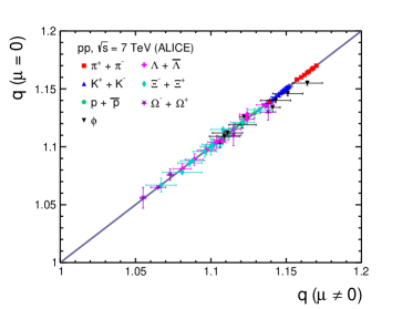
Figure 1: (Color online) Comparison of non-extensive parameter ($q$) at ($\mu=0$) and ($\mu\neq 0$) for $pp$ collisions at $\sqrt{s}$ = 7 TeV for different final state particles.

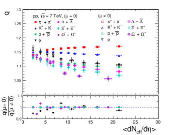
Figure 2: (Color online) Comparison of the non-extensive parameter ($q$) at ($\mu=0$) and ($\mu\neq 0$) for $pp$ collisions at $\sqrt{s}$ = 7 TeV for different final state particles as a function of final state multiplicity. Shown in the bottom panel is the ratio of both cases, which indicates that $q$ hardly depends on the chemical potential of the system.

Fig. 1 shows the variation of non-extensive parameter at ($\mu=0$) and ($\mu\neq 0$) for $pp$ collisions at $\sqrt{s}$ = 7 TeV for different final state particles. As in the formulation section of the article, we have mentioned that the value of the non-extensive parameter $q$ is kept fixed, and we perform the fit to the transverse momentum distributions to determine the parameters like $T$, $V$, and the chemical potential $\mu$. So to validate our method, we have plotted the value of $q$ for both the cases $\it{i.e.}$ $(\mu=0$) and ($\mu\neq 0$). This suggests the value of $q$ is independent irrespective of the value of $\mu$. The contribution of $\mu$ is taken care of by $T_{0}$ and $V_{0}$ as mentioned in Eqns. 3 and 4. We fitted the spectrum with $y=mx+c$, and found the parameters $m$ = 1.0 and the intercept $c=0$. Going one step further, we plot the variation of the $q$-parameter for both the cases of $\mu=0$ and $\mu\neq 0$ for all the considered particle species as a function of the final state-charged particle multiplicity. This is shown in Fig. 2. The bottom panel of which shows a ratio indicating a near-independency of the $q$-parameter on the chemical potential of the system. This justifies the procedure mentioned in the above section.

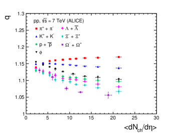
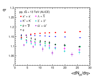
Figure 3: (Color online) Non-extensive parameter ($q$) as a function of charged-particle multiplicity for $pp$ collisions at $\sqrt{s}$ = 7 (left panel) and 13 TeV (right panel) for different final state particles.

In fig. 3, we use Eq. 5 to fit the transverse momentum spectra of various identified particles observed experimentally for different multiplicity classes at $\sqrt{s}$ = 7 TeV and $\sqrt{s}$ = 13 TeV. It illustrates the variation of non-extensive parameter ($q$) as a function of charged-particle multiplicity at $\sqrt{s}$ = 7 (left panel) and 13 TeV (right panel) for various final state particles. The value of $q$ decreases monotonically with an increase in multiplicity for all the particles, suggesting that the system created in higher multiplicity classes is close to thermal equilibrium. However, it can be observed that the value of $q$ is relatively independent of charged-particle multiplicity for pion. The decrease in $q$-values is an important observation as it infers that the hot and dense system formed in high multiplicities becomes close to a thermalized Boltzmann description of the system.

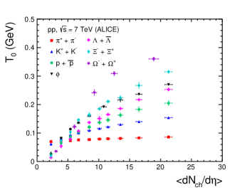
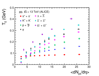
Figure 4: (Color online) Temperature ($T_{0}$) as a function of charged-particle multiplicity for $pp$ collisions at $\sqrt{s}$ = 7 (left panel) and 13 TeV (right panel) for different final state particles at zero chemical potential.

Further, fig. 4 represents the temperature parameter, ($T_{0}$) extracted from the fitting as a function of charged-particle multiplicity for $pp$ collisions at $\sqrt{s}$ = 7 (left panel) and 13 TeV (right panel) for different final state particles at zero chemical potential. We observe that with increasing charged-particle multiplicity, the temperature for all the hadrons increases. A mass-ordering in the trends can be observed in the figures with heavier mass particle having a higher temperature than a lighter mass particle at a certain charged particle multiplicity. This corresponds to a mass-dependent differential freeze-out scenario, where particles freeze-out at different times, corresponds to different volumes and temperatures for different particle species.

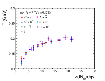
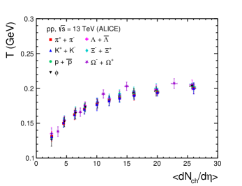
Figure 5: (Color online) Temperature ($T$) as a function of charged-particle multiplicity for $pp$ collisions at $\sqrt{s}$ = 7 (left panel) and 13 TeV (right panel) for different final state particles at the non-zero chemical potential.

Now, we use the $q$-values obtained from the first set of fits as fixed parameters for the second set of fits. In this case, the obtained parameters will change from $T_{0},R_{0}$ to $T$ and $R$, and the chemical potential is kept as a free parameter. In fig. 5, we show the temperature ($T$) at non-zero chemical potential as a function of charged-particle multiplicity for $pp$ at $\sqrt{s}$ = 7 (left panel) and 13 TeV (right panel) for various final state particles. We observe a monotonic increase in the temperature for all the hadrons as we move towards the higher charged multiplicity. If we consider a given charged-particle multiplicity, the temperature shows a weak particle species dependency in $pp$ collision for both the center-of-mass energies. It suggests that all the particles have the same kinetic freeze-out temperature for a certain charged-particle multiplicity. Similar results are obtained in ref. Khuntia:2018znt . At kinetic freeze-out, the observed particle-antiparticle symmetry only signifies that the chemical potentials for particles must be equal to those for antiparticles. However, they do not have to be zero due to the absence of chemical equilibrium at kinetic freeze-out.

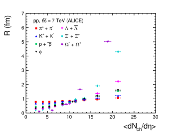
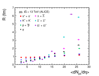
Figure 6: (Color online) Radius of the system ($R$) as a function of charged-particle multiplicity for $pp$ collisions at $\sqrt{s}$ = 7 TeV (left panel) and 13 TeV (right panel) for different final state particles.

Figure 6 shows the radius of the system ($R$) as a function of charged-particle multiplicity for $pp$ collisions at $\sqrt{s}$ = 7 (left panel) and 13 TeV (right panel) for different final state particles at non-zero $\mu$. We observe that the system’s radius for all the hadrons taken in this study is almost identical to a certain charged-particle multiplicity. After that, we see a particle species dependency in the value when we move toward the higher charged-particle multiplicity. Also, we observe that for lighter particles such as $\pi$, $K$, and $p$, the radius value is the same throughout.

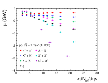
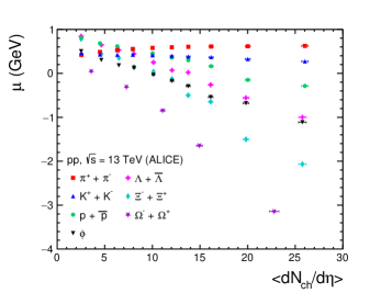
Figure 7: (Color online) Chemical potential ($\mu$) as a function of charged-particle multiplicity for $pp$ collisions at $\sqrt{s}$ = 7 (left panel) and 13 TeV (right panel) for different final state particles.

Figure 7 shows chemical potential ($\mu$) as a function of charged-particle multiplicity for $pp$ collisions at $\sqrt{s}$ = 7 (left panel) and 13 TeV (right panel) for different final state particles at a fixed value of non-extensive parameters. A non-zero value of the chemical potential at kinetic freeze-out temperature is observed for all the considered particle species. There is also a particle species dependency in the value of chemical potential for both the center-of-mass energies at the LHC. As we move towards massive particles, the chemical potentials go towards a negative value. However, we observe positive chemical potentials for all the charged-particle multiplicity for lighter particles such as $\pi$, $K$, and $p$. The observed values of chemical potential infer that there is no chemical equilibrium at the kinetic freeze-out, the values obtained for $\mu$ for different particle types vary considerably.

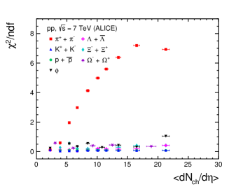
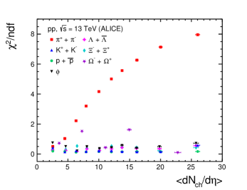
Figure 8: (Color online) $\chi^{2}/ndf$ as a function of charged-particle multiplicity for $pp$ collisions at $\sqrt{s}$ = 7 (left panel) and 13 TeV (right panel) for different final state particles.

In figure  8, $\chi^{2}/ndf$ as a function of charged-particle multiplicity for $pp$ collisions at $\sqrt{s}$ = 7 (left panel) and 13 TeV (right panel) for different final state particles at non-zero chemical potential is shown. The quality of the fits is given by the reduced $\chi^{2}$. This shows that the spectra are well described by the thermodynamically consistent form of Tsallis distribution. As the fit quality is very good up to 6 GeV in $p_{\rm T}$, the value of $\chi^{2}/ndf$ is always less than 1 except for $\pi$. We also did the $p$-value test of the fitting and got $p$-value equal to 1 for all the cases.

IV Summary

This article reviews another prospect to describe the kinetic freeze-out stage amidst significant chemical potential, specifically to explain the final state of the system produced in $pp$ collisions. A thorough analysis is presented, taking chemical potential into account in the Tsallis distribution Eq. (1) by following a two-step procedure. We have used the redundancy present in the variables $T$, $V$, $q$ and $\mu$ expressed in Eqns. (3) and (4) and performed all fits using Eq. (5), that is effectively establishing the chemical potential equal to zero. This study reviewed a comparison of $T$ and $T_{0}$ values for both the center-of-mass energies. This result confirms that the variables $T$, $V$, $q$, and $\mu$ in the Tsallis distribution function Eq. (1) have a redundancy for $\mu\neq 0$.

1. The non-extensive Tsallis distribution provides a good description of the $p_{\rm T}$-spectra of identified hadrons in $pp$ collisions.

2. The resulting temperatures, $T$, are the same for all particle species considered in this study. In contrast to the results obtained in  Bhattacharyya:2017hdc , the inconsistency can be traced back to the incorrect use of chemical potentials in the last analysis.

3. The decoupling temperature for all the particle species studied in this analysis seems to be the same when one considers a finite chemical potential at the kinetic freeze-out of the produced fireball.

4. The values obtained for $\mu$ for different particle species vary considerably and there is no chemical equilibrium at kinetic freeze-out in $pp$ collisions.

In this work, the importance of the chemical potential in the Tsallis distribution has been explored while analysing the identified particle spectra in $pp$ collisions. This leads to a detailed analysis of the various parameters in the new domain and confirms the usefulness of the Tsallis distribution in high-energy collisions.

References

- (1) M. Gyulassy and L. McLerran, Nucl. Phys. A 750, 30-63 (2005)
- (2) P. Braun-Munzinger and J. Stachel, Nature 448, 302-309 (2007)
- (3) B. V. Jacak and B. Muller, Science 337, 310-314 (2012)
- (4) N. Itoh, Prog. Theor. Phys. 44, 291 (1970)
- (5) J. C. Collins and M. J. Perry, Phys. Rev. Lett. 34, 1353 (1975)
- (6) N. Cabibbo and G. Parisi, Phys. Lett. B 59, 67 (1975)
- (7) G. Chapline and M. Nauenberg, Phys. Rev. D 16, 450 (1977)
- (8) A. Andronic, P. Braun-Munzinger, K. Redlich and J. Stachel, Nature 561, 321 (2018)
- (9) J. Sollfrank, P. Koch and U. W. Heinz, Phys. Lett. B 252, 256 (1990)
- (10) C. R. Allton, S. Ejiri, S. J. Hands, O. Kaczmarek, F. Karsch, E. Laermann, C. Schmidt and L. Scorzato, Phys. Rev. D 66, 074507 (2002)
- (11) C. R. Allton, S. Ejiri, S. J. Hands, O. Kaczmarek, F. Karsch, E. Laermann and C. Schmidt, Phys. Rev. D 68, 014507 (2003)
- (12) R. V. Gavai and S. Gupta, Phys. Rev. D 68, 034506 (2003)
- (13) C. R. Allton, M. Doring, S. Ejiri, S. J. Hands, O. Kaczmarek, F. Karsch, E. Laermann and K. Redlich, Phys. Rev. D 71, 054508 (2005)
- (14) A. Bazavov, H. T. Ding, P. Hegde, O. Kaczmarek, F. Karsch, E. Laermann, Y. Maezawa, S. Mukherjee, H. Ohno and P. Petreczky, et al. Phys. Rev. D 95, 054504 (2017)
- (15) K. Rajagopal and F. Wilczek, in At the Frontier of Particle Physics: Handbook of QCD ed. M. Shifman, p. 2061 (World Scientific, Singapore) (2001).
- (16) S. Acharya et al. [ALICE Collaboration], Phys. Lett. B 802, 135225 (2020).
- (17) D. Sahu, S. Tripathy, G. S. Pradhan and R. Sahoo, Phys. Rev. C 101, 014902 (2020).
- (18) R. Scaria, C. R. Singh and R. Sahoo, [arXiv:2208.14792 [hep-ph]].
- (19) B. I. Abelev et al. [STAR Collaboration], Phys. Rev. C 75, 064901 (2007).
- (20) A. Adare et al. [PHENIX], Phys. Rev. D 83, 052004 (2011)
- (21) A. Adare et al. [PHENIX], Phys. Rev. C 83, 064903 (2011)
- (22) V. Khachatryan et al. [CMS], JHEP 02, 041 (2010)
- (23) V. Khachatryan et al. [CMS], Phys. Rev. Lett. 105, 022002 (2010)
- (24) G. Aad et al. [ATLAS], New J. Phys. 13, 053033 (2011)
- (25) K. Aamodt et al. [ALICE Collaboration], Eur. Phys. J. C 71, 1655 (2011).
- (26) B. Abelev et al. [ALICE Collaboration], Phys. Lett. B 717, 162 (2012).
- (27) B. Abelev et al. [ALICE Collaboration], Phys. Lett. B 712, 309 (2012).
- (28) S. Chatrchyan et al. [CMS Collaboration], Eur. Phys. J. C 72, 2164 (2012).
- (29) J. Cleymans and D. Worku, J. Phys. G 39, 025006 (2012)
- (30) J. Cleymans and D. Worku, Eur. Phys. J. A 48, 160 (2012)
- (31) M. D. Azmi and J. Cleymans, Eur. Phys. J. C 75, 430 (2015)
- (32) G. Wilk and Z. Wlodarczyk, Phys. Rev. Lett. 84, 2770 (2000)
- (33) J. Cleymans, G. I. Lykasov, A. S. Parvan, A. S. Sorin, O. V. Teryaev and D. Worku, Phys. Lett. B 723, 351 (2013)
- (34) J. Cleymans and M. Wellington Paradza, MDPI Physics 2, 654 (2020)
- (35) J. Cleymans and M. W. Paradza, [arXiv:2010.05565 [hep-ph]].
- (36) A. Khuntia, H. Sharma, S. Kumar Tiwari, R. Sahoo and J. Cleymans, Eur. Phys. J. A 55, 3 (2019)
- (37) S. Acharya et al. [ALICE], Phys. Rev. C 99, 024906 (2019)
- (38) S. Acharya et al. [ALICE], Eur. Phys. J. C 80, 693 (2020)
- (39) S. Acharya et al. [ALICE], Phys. Lett. B 807, 135501 (2020)
- (40) S. Acharya et al. [ALICE], Eur. Phys. J. C 80, 167 (2020)
- (41) T. Bhattacharyya, J. Cleymans, L. Marques, S. Mogliacci, and M. W. Paradza, J. Phys. G 45, 055001 (2018)