Probing Pole Skipping through Scalar-Gauss-Bonnet coupling

Abstract

The holographic phenomena of pole skipping have been studied in the presence of scalar-Gauss-Bonnet interaction in four-dimensional Anti-de Sitter-Schwarzchild black hole background. Pole skipping points are special points in phase space where the bulk linearised differential equations have multiple ingoing solutions. Those special points are claimed to be connected to chaos. In this paper, we initiated a novel study on understanding the response of those special points under the application of external sources. The source is identified with the holographic dual operator of the bulk scalar field with its non-normalizable solutions. We analyze in detail the dynamics of pole skipping points in both sound and shear channels, considering linear perturbation in bulk. In the perturbative regime, characteristic parameters for chaos, namely Lyapunov exponent and butterfly velocity, remain unchanged. However, the diffusion coefficient has evolved non-trivially under the external source.

1 Introduction

Chaos, at the classical level, explains various macroscopic phenomena of hydrodynamics from a microscopic viewpoint. These phenomena are local criticality, zero temperature entropy, diffusion transport, Lyapunov exponent, and butterfly velocity. At the quantum level, chaos is similarly essential to studying those phenomena Gu:2016oyy ; Patel:2016wdy ; Grozdanov:2018atb . Recently, chaos in many body systems has drawn tremendous interest. It can be observed from the energy density two-point function. Since the holographic tools have an extensive advantage in studying those two-point functions from gravity theory, nowadays, the AdS/CFT correspondence Maldacena:1997re ; Aharony:1999ti is being used to describe the chaotic behavior in many-body quantum system Blake:2017ris ; Blake:2018leo ; Blake:2019otz ; Blake:2021hjj . However, using the holographic description, the microscopic behavior of quantum chaos was first established in Grozdanov:2017ajz . The two-point energy density function can be described with the four-point out-of-time-ordered correlator(OTOC).

$$\langle V(t,\vec{x})W(0)V(t,\vec{x})W(0)\rangle_{\beta_{0}}\approx e^{\lambda_{L}(t-|\vec{x}|/v_{B})}$$ (1.1)

where $\lambda_{L}$ is the Lyapunov exponent and $v_{B}$ is the butterfly velocity related to chaos. For a chaotic system, the two-point energy density function shows non-uniqueness around some special points in momentum space $(\omega,\,k)$. Holographically, the OTOC is non-uniquely defined at those points. These points are where the poles and zeros of the energy density function overlap. They are marked as the Pole-skipping (PS) points. For example, the boundary two-point (Green’s) function is a the ratio of the normalized mode to the non-normalized mode of the bulk field $\Phi$, which generally takes the form as $G_{R}\propto\frac{\Phi_{b}(\omega,k)}{\Phi_{a}(\omega,k)}$, At the pole-skipping point, $\Phi_{b}(\omega_{*},k_{*})=\Phi_{a}(\omega_{*},k_{*})=0$ and makes the Green’s function ill-defined. The line of poles is defined by $\Phi_{a}(\omega_{*},k_{*})=0$ whereas the line of zeros is given by $\Phi_{b}(\omega_{*},k_{*})=0$. Thus the pole-skipping points are some special locations in the $\omega-k$ plane. By analyzing the shock waves in an eternal black-hole background, chaos parameters are related to OTOC Shenker:2014cwa . At the above special points $(\omega_{*},k_{*})$ of energy-density two-point function, one can relate the parameters of chaos as,

$$\omega_{*}=i\lambda_{L},\hskip 28.45274ptk_{*}=\frac{i\lambda_{L}}{v_{B}}$$ (1.2)

where $\lambda_{L}$ and $v_{B}$ are the Lyapunov exponent and butterfly velocity associated with the considered chaotic system.

However, the behavior of the energy density function is universal for maximally chaotic systems. The microscopic dynamics of various hydrodynamic quantities are deeply related to the near-horizon analysis of holographic gravity. Indeed, the pole-skipping points can be identified from the in-going bulk field near the horizon. At those special points, the bulk field leads to the multi-valued Green’s function at the boundaryNatsuume:2019xcy . In simple words, there is no unique in-going solution at the horizon for those pole-skipping points. This holographic study has been performed for various bulk theories Natsuume:2019sfp ; Ahn:2019rnq ; Ahn:2020bks ; Blake:2021hjj ; Amano:2022mlu ; Sil:2020jhr ; Atashi:2022emh ; Yuan:2020fvv ; Kim:2020url ; Choi:2020tdj . In Ceplak:2019ymw ; Natsuume:2019xcy , the pole-skipping points have been found for the BTZ background. They have shown the intersection of the lines of poles and zeros and the existence of two regular in-going solutions near the horizon. The pole-skipping has been also studied with finite coupling correction Natsuume:2019vcv , with higher curvature correction Wu:2019esr and also in the case of zero temperature Natsuume:2020snz . Hydrodynamics transport phenomena have been studied with the pole-skipping Grozdanov:2018kkt ; Grozdanov:2019uhi ; Li:2019bgc ; Abbasi:2020ykq ; Abbasi:2020xli . Similar pole-skipping points have been also evaluated for the fermionic models Ceplak:2019ymw ; Ceplak:2021efc . In the above articles, we have seen some of the pole-skipping points in the $\omega-k$ plane located at $\text{Im}(\omega)$ are related to chaos. However, they follow the chaos bound Maldacena:2015waa . We have also seen that these special points describe various hydrodynamic mechanisms apart from chaos, e.g., the momentum density two-point function gives shear viscosity, diffusion modes, etc.

Higher curvature corrections and stringy correction to the pole-skipping have been explicitly studied Wu:2019esr ; Natsuume:2019vcv . Due to the effect of these corrections, the Lyapunov exponent and butterfly velocity have been modified. In this article, we discuss the effect of the higher order Gauss-Bonnet curvature term coupled with a scalar functional $\zeta(\phi)\sim\phi^{p}$ of a scalar field $\phi$, where $p$ is an integer. However, the effect of this coupling is considered to be so trivial that no back-reaction is included in the bulk solution. In the bulk theory, we take the standard four-dimensional Schwarzchild-Anti de-Sitter metric which asymptotically reduces to pure AdS. So, on the boundary, we have a Conformal Field Theory at a finite temperature which is maximally chaotic in nature. Therefore without modification (due to back-reaction) the chaos profile remains unaffected. In this background, we have studied the pole-skipping points for scalar and metric perturbations. We expect the effect of interaction on the pole-skipping points. We show this effect with respect to the variation of the source of the scalar field located on the boundary. We plot those effects for different powers $p$. In the sound channel, the flow and decay of energy density are expected to be affected by this interaction. Unlike the interaction-free background, we find decay in momentum density in the shear channel at a higher value of $p$. Here we have pointed out the variation of the diffusion coefficient with the scalar source. It also shows consistent behavior with the effect of interaction.

We briefly mention the result of this work as follows. We have noticed the effect of the interaction on the solution of the scalar field. To show this, we have plotted the values of the scalar $\phi$ at the horizon against its value on the boundary, i.e., scalar source $\mathcal{O}_{s}$. The relation between these two quantities has shown non-linearity for higher power $p$ of scalar. However, for a low regime of source value, it remains linear. Similarly in the pole-skipping points of the scalar field, we find an additional correction term in $k$ due to the interaction. Because of this correction, the imaginary value of $k$ decreases. As we are interested in the perturbative regime, we will not allow the scalar source to increase much. In all of the plots, we will take the maximum value of the scalar source in $\mathcal{O}(1)$. In the shear channel, we find a similar effect on $k$. However, for $p>3$, we find imaginary $k$ which implies the exponential decay or growth of the corresponding density function. Here we calculate the diffusion coefficient from the lowest point. It shows that the rate of diffusion decreases with the increase of scalar source and it is always below $1/4\pi T$ for $p>3$. On the other hand, in the sound channel, we find the effect of interaction for all $p>1$ are similar. In this channel, without interaction, $k^{4}$ has pure real ($<0$) values. Due to interaction, it encounters an imaginary part which increases with the effect of the scalar source. As the real $k^{4}<0$ gives $k$ with equal real and imaginary parts indicating the energy transport and decay/growth of energy density respectively. With the effect of interaction, the real and imaginary parts of $k$ become unequal. Thus one can conclude this is a result of the variation of thermal transport due to interaction.

We have organized the paper as follows. In section 2, we briefly describe our model, showing Einstein’s equation and background metric. We have also talked about the behaviour of the background scalar field and calculated the source and condensation values. In section 3, we have studied pole-skipping for scalar field perturbation. The metric perturbations – shear and sound modes – have been discussed in section 4. In the following section, we have calculated the chaos-related parameters, first, from the perturbed $vv$ component and then from the master equation. Finally, we concluded our results with a brief overview of the paper in section 6.

2 Holographic Gravity Background

Now, in the holographic model, as we want to study pole-skipping at finite temperatures, we need to use a black hole solution in bulk. We consider a four-dimensional Anti-de Sitter Schwarzchild black hole. Holographically, the boundary theory is three-dimensional gauge theory. The bulk metric asymptotically gives $(3+1)$ dimensional AdS space. So, the corresponding boundary theory is a finite temperature field theory. Initially, we consider pure black hole solution and associated Einstein’s action in the bulk theory as,

$$\mathcal{S}_{EH}=\int d^{4}x\sqrt{-g}\left(\kappa\mathcal{R}+\Lambda\right)$$ (2.1)

where $\kappa=(16\pi G_{N})^{-1}$ is a constant related to the four-dimensional Newton’s constant with mass dimensions $2$ (here we set it to unity.). The associated field equation

$$\mathcal{G}_{\mu\nu}\equiv\mathcal{R}_{\mu\nu}-\frac{1}{2}\mathcal{R}g_{\mu\nu}=\frac{1}{2\kappa}\Lambda g_{\mu\nu}$$ (2.2)

gives the $3+1$ dimensional AdS-Schwarzchild black hole solution

$$ds^{2}=L^{2}\left[-r^{2}f(r)dt^{2}+\frac{dr^{2}}{r^{2}f(r)}+h(r)\left(dx^{2}+dy^{2}\right)\right]$$ (2.3)

$$f(r)=1-\left(\frac{r_{0}}{r}\right)^{3},\quad\quad h(r)=r^{2}$$

Where $L$ is the AdS radius. In the Einstein action, $R$ is the Ricci scalar of the background (2.3) and $\Lambda$ is related to the cosmological constant in four dimensions. In our case, $\Lambda=6\kappa/L^{2}$ and $r$ is the radial coordinate of the black hole with the horizon radius $r_{0}$. The horizon radius is related to the temperature $T$ of the black hole as $4\pi T=r_{0}^{2}f^{\prime}(r_{0})=3r_{0}$, where prime denotes derivative w.r.t. $r$.

Now in the action (2.1), we have added a perturbative term $\frac{1}{2}\alpha^{\prime}\zeta(\phi)\mathcal{R}_{GB}$, where $\alpha^{\prime}$ is arbitrary coupling constant which is very small ($\ll 1$) real number. It acts as the perturbation parameter. $\zeta(\phi)$ is a dimensionless real scalar functional of the minimally coupled scalar field $\phi$ of mass $m$. In this present study, we have considered $\zeta(\phi)=L^{p}\phi^{p}$, $p\in\mathbb{Z}^{+}$. In this present discussion, we will consider $L=1$. The term $\mathcal{R}_{GB}$ is the higher-ordered Gauss-Bonnet curvature term (in $4d$), which is coupled to the scalar $\phi(r)$ through $\zeta$. Gauss-Bonnet term can be written as,

$$\mathcal{R}_{GB}=\mathcal{R}_{\mu\nu\rho\sigma}\mathcal{R}^{\mu\nu\rho\sigma}-4\mathcal{R}_{\mu\nu}\mathcal{R}^{\mu\nu}+\mathcal{R}^{2}.$$

With this scalar-Gauss-Bonnet interaction term, the background action takes the following form as

$$\mathcal{S}=\int d^{4}x\sqrt{-g}\left[\kappa\mathcal{R}+\Lambda+\frac{\alpha^{\prime}}{2}\zeta(\phi)\mathcal{R}_{GB}\right].$$ (2.4)

For $p=0$, pole-skipping has been exclusively studied previously in the five dimensions Wu:2019esr and it has considered the back-reaction of the higher curvature on the background. In our study, we are interested in $p\neq 0$ cases and treating $\alpha^{\prime}$ as a perturbative parameter, our background will remain unaffected by the back-reaction of the scalar field. Now taking the variation of the metric tensor in (2.4), we get the Einstein equation as follows

$$(\kappa-2\alpha^{\prime}\nabla_{\rho}\nabla^{\rho}\zeta(\phi))\mathcal{G}_{\mu\nu}-\frac{1}{2}g_{\mu\nu}(\Lambda+\frac{1}{2}\alpha^{\prime}\zeta(\phi)\mathcal{R}_{GB})+\alpha^{\prime}\zeta(\phi)\left(\mathcal{R}_{\mu}^{\leavevmode\nobreak\ \rho\sigma\tau}\mathcal{R}_{\nu\rho\sigma\tau}-4\mathcal{R}_{\rho\mu}\mathcal{R}^{\rho}_{\nu}+\mathcal{R}\mathcal{R}_{\mu\nu}\right)$$ (2.5)

$$-\alpha^{\prime}\left(\mathcal{R}\nabla_{(\mu}\nabla_{\nu)}\zeta(\phi)-4\mathcal{R}_{\rho(\mu}\nabla_{\nu)}\nabla^{\rho}\zeta(\phi)+2\left(g_{\mu\nu}\mathcal{R}_{\rho\sigma}+\mathcal{R}_{\mu(\rho\sigma)\nu}\right)\nabla^{\rho}\nabla^{\sigma}\zeta(\phi)\right)=0$$ ,

where $\mathcal{G}_{\mu\nu}$ is the Einstein tensor.

The aforementioned scalar field $\phi$ is a minimally coupled scalar in the black hole background (2.1). In the interaction term, the scalar couples with the second-order curvature terms. Taking this curvature coupling into account the Klein-Gordon equation of $\phi$ becomes,

$$\frac{1}{\sqrt{-g}}\partial_{\mu}\left(\sqrt{-g}g^{\mu\nu}\partial_{\nu}\phi\right)-m^{2}\phi+\frac{\alpha^{\prime}}{2}\mathcal{R}_{GB}\frac{\partial}{\partial\phi}\zeta(\phi)=0$$ (2.6)

Our aim would be to compute the near horizon in going modes and their properties. Therefore, it is fruitful to perform our calculations in the ingoing Eddington-Finkelstein co-ordinate. So, we consider $v=t+r_{*}$, where $v$ is the null co-ordinate and $r_{*}$ is the tortoise co-ordinate. The metric (2.3) transforms into,

$$ds^{2}=-r^{2}f(r)dv^{2}+2dvdr+r^{2}\left(dx^{2}+dy^{2}\right).$$ (2.7)

The metric (2.3) is singular at $r=r_{0}$. In this new coordinate, the apparent singularity is removed. The metric has rotational symmetry in the $(x,y)$ plane. In the background (2.7),

$$\mathcal{R}=-12,\quad\quad\mathcal{R}_{GB}(r)=12\left(2+\frac{r_{0}^{6}}{r^{6}}\right).$$

At horizon, $\mathcal{R}_{GB}(r_{0})=36$ and at the boundary $\mathcal{R}_{GB}(r\to\infty)\approx 24$. So, in the action (2.4), the scalar-Gauss-Bonnet interaction term can be considered as perturbation if $\alpha^{\prime}\ll 1$ where the scalar is assumed to be constant of $\mathcal{O}(1)$ at both ends.

In this background, the Klein-Gordon equation turns out to be,

$$r^{2}f(r)\phi^{\prime\prime}(r)+\left(r^{2}f^{\prime}(r)+4rf(r)\right)\phi^{\prime}(r)-m^{2}\phi(r)+\frac{\alpha^{\prime}}{2}\mathcal{R}_{GB}\frac{\partial}{\partial\phi}\zeta(\phi)=0.$$ (2.8)

The asymptotic $(r\rightarrow{\infty})$ behavior of equation (2.8) gives the following

$$\lim_{r\rightarrow\infty}\phi(r)=\mathcal{O}_{s}r^{\Delta-3}+\mathcal{O}_{c}r^{-\Delta}.$$ (2.9)

Where, at infinity (where is our boundary), the leading coefficient $\mathcal{O}_{s}$ is the source, and the subleading coefficient $\mathcal{O}_{c}$ is the condensation of the dual boundary dual operator. The scaling dimension of the dual operator $\Delta={3}/{2}+\sqrt{{9}/{4}+m^{2}}$. There is a lower bound on the scalar mass called the bound of BF (Breitenlohner and Freedman) which states that $m^{2}\geq-{d^{2}}/{4}$ for $(d+1)$ gravitational background. Otherwise, the background solution will be unstable. In our case, this bound will be $m^{2}>-{9}/{4}$. From equation (2.9), we can write,

$$\lim_{r\rightarrow\infty}r\phi^{\prime}(r)=(\Delta-3)\mathcal{O}_{s}r^{\Delta-3}-\Delta\mathcal{O}_{c}r^{-\Delta}.$$ (2.10)

Now, we can easily get the source and condensation from equations (2.9) and (2.10) by some algebra as shown in Chakrabarti:2019gow as

$$\mathcal{O}_{s} =\lim_{r\rightarrow\infty}\frac{r^{3-\Delta}\left(\Delta\phi(r)+r\phi^{\prime}(r)\right)}{2\Delta-3}$$ (2.11)

$$\mathcal{O}_{c} =\lim_{r\rightarrow\infty}\frac{r^{\Delta}\left((\Delta-3)\phi(r)-r\phi^{\prime}(r)\right)}{2\Delta-3}.$$ (2.12)

Since our background is neutral, the scalar field will not form any condensation. Rather, in the next sections, we will mainly see the effect of the source in the channels.

3 Scalar field perturbation

In this section, we study the dispersion relation associated with the scalar field $\phi$ which is a minimally coupled scalar with mass $m$. This scalar field $\phi$ is regular at the horizon and decays in the asymptotic limit. With these conditions, the solution of the scalar can be found from the equation (2.8). Now assuming the scalar field is a function of the radial coordinate $r$ only, i.e., $\zeta(\phi)=\phi(r)^{p}$. We take the near-horizon expansion of the field as

$$\phi(r)=\sum_{n=0}^{\infty}\phi^{(n)}(r_{0})\times(r-r_{0})^{n}=\phi(r_{0})+\phi^{\prime}(r_{0})(r-r_{0})+\phi^{\prime\prime}(r_{0})(r-r_{0})^{2}+\cdots$$

where, $\phi^{(n)}\equiv\frac{d^{n}\phi(r)}{dr^{n}}|_{r=r_{0}}$. From these series, the first three derivatives of $\phi$ at $r=r_{0}$ can be found as,

$$\phi^{\prime}\left(r_{0}\right) = \frac{m^{2}\phi\left(r_{0}\right)-18\alpha^{\prime}p\phi\left(r_{0}\right)^{p-1}}{3r_{0}}$$

$$\phi^{\prime\prime}\left(r_{0}\right) = \frac{-18\alpha^{\prime}p\left(pm^{2}-12\right)\phi\left(r_{0}\right)^{p-1}+m^{2}\left(m^{2}-6\right)\phi\left(r_{0}\right)}{18r_{0}^{2}}$$

$$\phi^{\prime\prime\prime}\left(r_{0}\right) = \frac{1}{162r_{0}^{3}}\left[-18\alpha^{\prime}p\left((2(p-2)p+3)m^{4}+6(3-7p)m^{2}+432\right)\phi\left(r_{0}\right)^{p-1}\right.$$

$$\left.\quad\quad\quad\quad\quad+m^{2}\left((m^{2}-6)(m^{2}-9)-3(m^{2}-18)\right)\phi\left(r_{0}\right)\right]$$

Similarly, we can also find the higher order derivatives in terms of $\phi(r_{0})$.

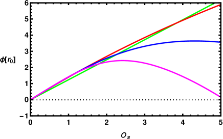
Figure 1: Left: The plot of $\mathcal{O}_{s}$ vs $\phi(r_{0})$ for $p=2$ (green color), $p=3$ (red color), $p=4$ (blue color) and $p=5$ (magenta color). Here we have taken scalar mass $m^{2}=-2$, $\alpha^{\prime}=0.001$, and $r_{0}=1$.

We can solve the scalar field from (2.8) numerically by providing some horizon value to the scalar field. From this solution, we can evaluate $\mathcal{O}_{s}$ and $\mathcal{O}_{c}$ as shown in (2.11). For the near horizon study, the regularity condition of the scalar field on the horizon is very important. So, for numerical evaluation of the source $\mathcal{O}_{s}$ or to get a consistent solution of $\phi(r)$; $\phi(r_{0})$ should be finite and small enough so that the near-horizon expansion remains convergent. From the plot of $\phi(r_{0})$ vs $\mathcal{O}_{s}$, we can say that at lower values of source $\mathcal{O}_{s}$, the relation between these two quantities is almost linear. But at higher values it becomes non-linear and the degree of non-linearity strongly depends on the power ($p$) of the interaction. Due to this fact, in this present work, we will confine our all numerical calculations to the low-value regime of the $\mathcal{O}_{s}$ or $\phi(r_{0})$.

Now to study the dispersion relation of the scalar field, we take the perturbation $\phi(r)\to\phi(r)+e^{-i\omega v+ikx}\varphi(r)$. The linearized equation from (2.8) is

$$r^{2}f(r)\varphi^{\prime\prime}(r)+\left(r^{2}f^{\prime}(r)+4rf(r)-2i\omega\right)\varphi^{\prime}(r)+$$

$$\quad\quad\quad\quad\left(6\alpha^{\prime}(p-1)p\left(f(r)^{2}-2f(r)+3\right)\phi(r)^{p-2}-\frac{k^{2}+m^{2}r^{2}+2ir\omega}{r^{2}}\right)\varphi(r)=0$$ (3.1)

Expanding the solution near the horizon $r=r_{0}$ and using the matrix method as given in Ceplak:2019ymw , we get the pole skipping points $(\omega,k)$. We find the lowest order point is $\omega_{1}=-\frac{3}{2}ir_{0}=-2i\pi T$ and

$$k_{1}^{2}+r_{0}^{2}\left(m^{2}-18\alpha^{\prime}p(p-1)\phi\left(r_{0}\right)^{p-2}+3\right)=0$$

Without any perturbation ($\alpha^{\prime}=0$), we get the results for pure Schwarzchild black hole $k_{1}^{2}=-(3+m^{2})r_{0}^{2}$, i.e., $k_{1}$ is completely imaginary. But, due to the effect of the interaction, $k_{1}$ can be real after a particular value of $\mathcal{O}_{s}$. Similar behaviour is also found for the higher-order pole-skipping points. Though we keep $\alpha^{\prime}$ small enough in the perturbative regime, $k_{1}^{2}$ becomes positive as the scalar source increases. So $k$ becomes real. From the equation of the perturbed scalar (3), it is clear to predict that for $p=0$ and $1$, there is no effect on $(\omega,k)$, i.e., we get the values of the black hole background without any perturbation. For $p\geq 2$, $p$ effects $k_{1}$ in similar way as $\alpha^{\prime}$ does. For the small enough $\mathcal{O}_{s}$, we have found $k$ in the imaginary plane which has been plotted in the left panel of Figure 2.

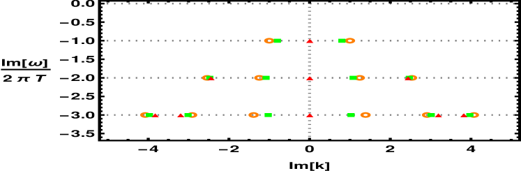
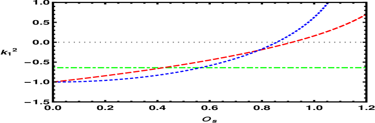
Figure 2: Left: The plot of $\frac{\text{Im}\left[\omega\right]}{2\pi T}$ vs $\text{Im}\left[k\right]$ at $\alpha^{\prime}=0.01$ for $p=1$ (orange circle), $p=2$ (green rectangle) and $p=3$ (red triangle). Right: The plot of $k_{1}^{2}$ vs $\mathcal{O}_{s}$ for $p=2$ (green dot-dashed line), $p=3$ (red dashed line) and $p=4$ (blue dotted line). Here we have taken scalar mass $m^{2}=-2,\,\alpha^{\prime}=0.01$ and $r_{0}=1$.

Here we have plotted first three poles $(\omega,k)$ in the complex plane for $p=1,\,2\,\&\,3$. For $p=1\,\&\,2$, we have found $2n$-number of points for $k_{n}$, i.e., $n$ number of complex roots for $k_{n}$. However, for $p=3$, we have found one real and $n-1$ complex root of each $k_{n}$. Because of these real roots, we have three points on the $\text{Im}(k)$ axis. For $p=2$, the interaction imposes a constant shift in $k$. But for $p\geq 3$ the shift due to the interaction is proportional to the source. So, as the source goes to zero, $k_{n}$ becomes the same as the pure AdS black hole. These have been shown in the right panel of the same figure. Here, we have presented the variation of $k_{1}^{2}$ with the scalar source $\mathcal{O}_{s}$ for $p=2,\,3\,\&\,4$. It is found that $k_{1}$ becomes real-valued above a certain value of $\mathcal{O}_{s}$. Now, if we allow only the imaginary values of $k_{1}$, we need to put a cutoff on $\mathcal{O}_{s}$. The same behaviour can be found for the higher order $k$. However as we go to higher order in poles or in interaction, we need to impose a smaller cutoff on the source value to get the pure imaginary root of $k$.

4 Metric perturbations

In the pole-skipping phenomena, we study the properties of the stress-energy tensor of the boundary field theory. Now with AdS/CFT duality, the bulk fields are mapped to boundary operators. Therefore, the boundary stress-energy tensors are associated with the metric perturbation of the bulk. In our bulk, we consider the metric perturbation

$$g_{\mu\nu}\to g_{\mu\nu}+e^{-i\omega v+ikx}\delta g_{\mu\nu}(r),$$ (4.1)

where $\omega$ and $k$ are energy and momentum parameters of the fluctuation and the fluctuation propagates radially. So, in the boundary field theory, we have the two points correlators which are $<T_{vv},T_{vv}>$, $<T_{vv},T_{vx}>$, $<T_{vv},T_{xx}>$, $<T_{vv},T_{yy}>$ in longitudinal mode and $<T_{vy},T_{vy}>$, $<T_{vy},T_{xy}>$, $<T_{xy},T_{xy}>$ in a transverse mode where $T_{\mu\nu}$ is the stress-energy tensor on the boundary. The metric perturbation: $\delta g_{vv},\,\delta g_{vx},\,\delta g_{xx},\,\delta g_{yy}$ and $\delta g_{vy},\,\delta g_{xy}$ are associated to the above two modes respectively. We impose the radial gauge condition $\delta g_{r\mu}=0$ for all $\mu$. We also use the traceless perturbation for simplicity, i.e., $g^{\mu\nu}\delta g_{\mu\nu}=0$ which gives $\delta g_{yy}=-\delta g_{xx}$. However the longitudinal modes are actually the scalar modes, it does not couple with a minimally coupled scalar. Therefore we can perturb only $g_{\mu\nu}$ without effecting $\phi$. Finally, we have three independent perturbations in longitudinal mode and two in transverse mode.

4.1 Shear Channel

As the momentum vector $(\omega,k)$ of the metric fluctuation is taken along $(v,x)$-plane, for shear mode, we consider the components coupled to $y$-direction. Here we take $g_{xy}$ and $g_{vy}$ as the only non-vanishing perturbations and these are completely decoupled from the longitudinal perturbations. These are associated with $T_{vy}$, $T_{xy}$ on the boundary. The linearised Einstein equations will give the dynamics of these fluctuations. At some special values of $(\omega,\,k)$, the solution of those equations near the horizon becomes non-unique and gives more than one independent solution. Those special points $(\omega,\,k)$ in this holographic gravity background are connected to the coincidence of poles and zeros of the boundary Greens function, $G_{\mu y,\nu y}$ where $\mu,\,\nu=v,\,x$.

Now we put these perturbations in the metric (2.7) and find the linearised form of the field equation (2.5) with only non-vanishing perturbations $g_{xy}$ and $g_{vy}$. We find that $vy,\,ry$ and $xy$ components of the linearised equations are only non-trivial, whereas other equations are self-satisfied. Out of these three equations, we find two coupled second-order differential equations as $\delta g_{vy}^{\prime\prime}(r)=f_{1}\left(\delta g_{vy}^{\prime},\,\delta g_{vy},\,\delta g_{xy}\right)$ and $\delta g_{xy}^{\prime\prime}(r)=f_{2}\left(\delta g_{vy}^{\prime},\,\delta g_{vy},\,\delta g_{xy}\right)$. Again, under diffeomorphism transformation with the vector field $e^{-i\omega v+ikx}\xi^{\mu}$, one can show that $\delta g_{vy}$ and $\delta g_{xy}$ will form a gauge invariant combination $\mathcal{Z}_{sh}$ as,

$$\mathcal{Z}_{sh}=\frac{1}{r^{2}}\left(\omega\delta g_{xy}+k\delta g_{vy}\right).$$

So, two second-order differential equations (DE) of $\delta g_{vy}$ and $\delta g_{xy}$ combine into a single second-order DE of $\mathcal{Z}_{sh}$. The final master equation is

$$\mathcal{M}_{sh}\mathcal{Z}^{\prime\prime}_{sh}(r)+\mathcal{P}_{sh}\mathcal{Z}^{\prime}_{sh}(r)+\mathcal{Q}_{sh}\mathcal{Z}_{sh}(r)=0.$$ (4.2)

Where, the coefficients $\mathcal{M}_{sh},\,\mathcal{P}_{sh}$ and $\mathcal{Q}_{sh}$ are functions of $\omega,k$ and $\phi(r)$. The details expressions are given in Appendix A. There we have considered the coefficients up to $\alpha^{\prime}$ order. As $\alpha^{\prime}=0$ the master equation reduces to the same as the pure AdS black hole. The near horizon structure of the master variable is taken as follows.

$$\mathcal{Z}_{sh}=\sum_{n=0}Z_{n}\times(r-r_{0})^{n}.$$

Now we expand the master equation (4.2) around $r=r_{0}$. At zeroth order $\mathcal{O}((r-r_{0})^{0})$, it gives the linear algebraic equation of $Z_{0}$ and $Z_{1}$. The coefficients of $Z_{0}$ and $Z_{1}$ are functions of two primary variables $\omega$ and $k$. So, at a particular point, $\omega=\omega_{1}$ the vanishing of the coefficient of $Z_{1}$ indicates that $Z_{1}$ is arbitrary. Again at the same $\omega$ value, we find a special value of $k=k_{1}$ where the coefficient of $Z_{0}$ vanishes. Therefore at the point $(\omega_{1},\,k_{1})$ the near horizon solution of $\mathcal{Z}_{sh}$ is defined with two arbitrary parameter $Z_{0},\,Z_{1}$ and the solution is combination of two arbitrary solutions $C_{1}(r-r_{0})Z_{0}+C_{2}(r-r_{0})Z_{1}$. So we find a non-unique solution at the point $(\omega_{1},\,k_{1})$ – which is the first order pole-skipping point. Here we find $\omega_{1}=-\frac{3}{2}ir_{0}$ and

$$k_{1}^{2}=3r_{0}^{2}\left[1-3\alpha^{\prime}\phi(r_{0})^{p}\frac{\xi(2\xi^{2}-\xi-17)}{2\xi+1}\right]$$ (4.3)

where, $\xi=mp^{2}/3$. We find $\omega_{1}$ same as the previous result Blake:2019otz for AdS₄ black hole. But $k_{1}$ contains a non-trivial shift due to the interaction. At $\alpha^{\prime}=0$, it gives the same $k_{1}^{2}$ as given in Blake:2019otz . With nonzero $\alpha^{\prime}$, the shift in momentum depends on the details properties of the scalar field and its interaction namely, power $p$ of the interacting field $\phi$, the value of the field at horizon $\phi(r_{0})$ and mass of it $m$. Now the scalar mass $m$ can not be zero to get the nonzero shift. Also, we need to maintain the value of $\alpha^{\prime}$ in such a way that the shift remains small enough, i.e., the absolute value of the correction term inside the square bracket in (4.3) is always less than unity. Next few higher-order pole-skipping points are $\omega_{n}=-\frac{3}{2}inr_{0}$ for $n=2,\,3,\dots$ and

$$k_{2}^{2} = 3\sqrt{2}r_{0}^{2}\left[1-\frac{3\alpha^{\prime}\xi\phi(r_{0})^{p}}{4(2\xi+1-\sqrt{2})^{2}}\left(12\xi^{4}+4(21-\sqrt{2})\xi^{3}+(209-74\sqrt{2})\xi^{2}\right.\right.$$ (4.4)

$$\left.\left.\hskip 170.71652pt+(134-238\sqrt{2})\xi+136+20\sqrt{2})\right)\right]$$

$$k_{3}^{2} = 3\sqrt{3}r_{0}^{2}\left[1+\frac{\xi(5-\sqrt{3})}{66(6\xi-3+2\sqrt{3})^{3}}\left(-3888\xi^{6}+54432\xi^{5}-(32400-21528\sqrt{3})\xi^{4}\right.\right.$$ (4.5)

$$+(976140-224964\sqrt{3})\xi^{3}-(1108017-786374\sqrt{3})\xi^{2}+(1134059-427507\sqrt{3})\xi$$

$$\hskip 199.16928pt\left.\left.+295381\sqrt{3}-222201\right)\right]$$

and so on. In all of these $k$ values, the absolute value of the perturbative correction increases with $\phi(r_{0})$ or the source $\mathcal{O}_{s}$ but the sign of the term is solely decided by the factor $pm^{2}$. We find that $k_{n}^{2}$ can be both greater or less than $3\sqrt{n}r_{0}^{2}$ depending on the value of $pm^{2}$. For example $k_{1}^{2}>3r_{0}^{2}$ for $\frac{3}{4}\left(1-\sqrt{137}\right)\leq m^{2}p<-\frac{3}{2}$ and $-\frac{9}{4}\leq m^{2}\leq-\frac{5}{4}$. However, for other higher mode points $k_{n}^{2}$ is always less than $3\sqrt{n}r_{0}^{2}$. It puts no further restriction on scalar mass.

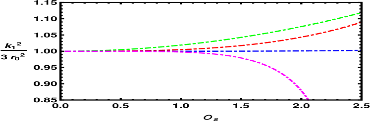
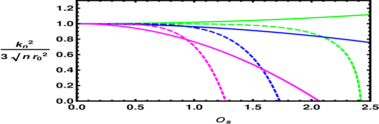
Figure 3: Left: The plot of $\frac{k_{1}^{2}}{3r_{0}^{2}}$ vs $\mathcal{O}_{s}$ where $p=2$ (green color), $p=3$ (red color), $p=4$ (blue color), and $p=5$ (magenta color). Right: The plot of $\frac{k_{n}^{2}}{3\sqrt{n}r_{0}^{2}}$ vs $\mathcal{O}_{s}$ for $n=1$ (green color), $n=2$ (blue color), $n=3$ (magenta color) and for two different powers $p=2$ (solid line) and $p=5$ (dashed line). Here we have taken $\alpha^{\prime}=0.001$ and $m^{2}=-2.0$.

In Figure 3, we have plotted $\frac{k_{1}^{2}}{3r_{0}^{2}}$. The ratio has been varied with the scalar source $\mathcal{O}_{s}$ for four different order of interaction $p=2,\,3,\,4\,\&\,5$ with perturbation parameter $\alpha^{\prime}=0.001$ and scalar mass $m^{2}=-2$. Fig.3 depicts that while the source is off the ratio is equal to unity. As the source increases from zero, the ratio deviates from unity and increases or decreases according to the power of the Scalar-Gauss-Bonnet interaction term $p$. At the given mass value, for $0<p\leq 4$, the ratio increases with source, and for $p\geq 5$ the ratio decreases from unity. The same has been depicted in the left panel of the figure. Whereas on the right panel of the same figure, $k_{1}^{2}/(3r_{0}^{2})$, $k_{2}^{2}/(3\sqrt{2}r_{0}^{2})$ and $k_{3}^{2}/(3\sqrt{3}r_{0}^{2})$ have been varied with the scalar source for $p=2$ and $p=5$. $k_{1}^{2}/(3r_{0}^{2})$ increases with source $\mathcal{O}_{s}$ for $p=2$ and decreases for $p=5$ which is consistent with analytical observations as discussed above. On the other hand, $k_{2}^{2}/(3\sqrt{2}r_{0}^{2})$ and $k_{3}^{2}/(3\sqrt{3}r_{0}^{2})$ decrease with source for both $p=2\,\&\,5$.

It has already been observed that for pure Schwarzchild-AdS₄ background, the first order pole-skipping point obeying the dispersion relation $\omega=-i\mathcal{D}_{s}k^{2}$ emerges from the boundary Greens function Blake:2019otz . However, the first pole-skipping point gives an upper bound on the diffusion constant Huh:2021ppg ; Hartman:2017hhp . The diffusion constant is related to the first order pole-skipping as $\mathcal{D}_{s}=\frac{i\omega_{1}}{k_{1}^{2}}$. Here, in our case, we find the diffusion constant $\mathcal{D}_{s}$ as

$$\mathcal{D}_{s}=\frac{i\omega_{1}}{k_{1}^{2}}=\frac{1}{2r_{0}}\left[1+3\alpha^{\prime}\phi(r_{0})^{p}\frac{\xi(2\xi^{2}-\xi-17)}{2\xi+1}\right]$$ (4.6)

Its upper bound is $\mathcal{D}_{s}(\alpha^{\prime}\neq 0)<\mathcal{D}_{s}(\alpha^{\prime}=0)$. For $d+2$ dimensional pure AdS-Schwarzchild black hole, the diffusion constant is bounded as $1\leq 4\pi\mathcal{D}_{s}T\leq\frac{d+1}{d}$. If the scalar field follows the BF bound and unitarity condition, the scalar mass follows the bound $-2.25<m^{2}<-1.25$. $\mathcal{D}_{s}T$ in (4.6) can be found in $1\leq 4\pi\mathcal{D}_{s}T\leq\frac{3}{2}$ for all $p\leq 6$ for the mass ranges given in Table 1.

Table 1: The mass range associated to $p$ to follow the allowed bound of the diffusion coefficient

Interaction order $p$ ($\phi^{p}$)	mass range
$p=1$	$-2.25<m^{2}<-1.5$
$p=2$	$-2.25<m^{2}<-1.25$
$p=3$	$-2.25<m^{2}<-1.25$
$p=4$	$-2.007<m^{2}<-1.25$
$p=5$	$-1.605<m^{2}<-1.25$
$p=6$	$-1.338<m^{2}<-1.25$

In the allowed mass range, the diffusion constant violates the bounds for $p\geq 7$.

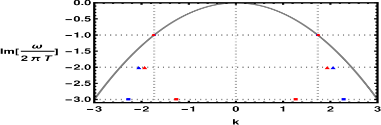
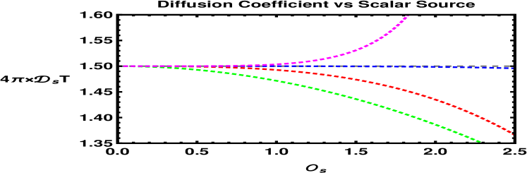
Figure 4: Left: The plot of PS points in $\omega-k$ plane for $\alpha^{\prime}=0$ (blue color) and $\alpha^{\prime}=0.001$ (red color), $\phi(r_{0})=1.1,\,p=3$ and $m^{2}=-2$. Three different shapes have been used for three different modes. The solid curve (gray color) is $\omega=\frac{-ik^{2}}{4\pi T}$. Right: Plot of $4\pi\mathcal{D}_{s}T$ vs $\mathcal{O}_{s}$ for $p=2$ (green line), $p=3$ (red line), $p=4$ (blue line) and $p=5$ (magenta line) $m^{2}=-2.0$ and $\alpha^{\prime}=0.001$.

In Figure 4, the left panel have shown the plot of the pole-skipping points in the $\omega-k$ plane. Here we have plotted the standard dispersion relation of the boundary theory in a low-frequency regime, $\omega(k)=-i\mathcal{D}_{s}k^{2}$ where $\mathcal{D}_{s}=\frac{1}{4\pi T}$ given in Blake:2019otz . When $\alpha^{\prime}=0$ or the perturbative correction is very small, the first pole-skipping point falls on the dispersion curve. As the effect of interaction increases the first pole-skipping point skips the dispersion curve. However, the other pole-skipping points always stay away from the dispersion curve. At the right panel of Figure 4, we have plotted the diffusion constant obtained in (4.6). Here the $4\pi\mathcal{D}_{s}T$ have been varied with the scalar source for three different $p$ values. As the source is zero the diffusion constants for all $2\leq p\leq 6$ become equal to the upper bound $\frac{3}{8\pi T}$. In the plot, as the source increases from zero, the diffusion constants start falling from the highest bound. For the coupling function $\zeta(\phi)\sim\phi^{2}$ and $\phi^{3}$, the diffusion constant decreases monotonically. At a particular value of the source, $4\pi\mathcal{D}_{s}T$ has become equal to unity, and for further increase of source value, it has fallen below its lower bound. However, for $p=4$, the diffusion constant is found to remain very close to its upper bound for a comparatively long range of $\mathcal{O}_{s}$. After that, it started decreasing very rapidly and reached below $1$. At these higher values of the source, the diffusion constant for $p=4$ has two different values for a single value of scalar source $\mathcal{O}_{s}$. It seems unusual. So we should control the source not to exceed $\sim 3$. Again though we know that the diffusion constant should not violate its lower bound, our results are not unphysical. Since our whole calculation is assumed to be in a perturbative regime, we are free to choose any tiny value of $\alpha^{\prime}$ and any small range of the scalar source for the numerical evaluation. Thus the better estimation in our case always makes $1\ll 4\pi\mathcal{D}_{s}T\leq\frac{3}{2}$ for $1<p\leq 6$.

4.2 Sound Channel

The longitudinal components of the metric perturbation are called the scalar or sound modes of the perturbation. These are associated with the energy density correlation on the boundary. The corresponding stress-energy tensor in this mode are $T_{vv},\,T_{vx},\,T_{xx}$ and $T_{yy}$ on the boundary field theory. These make the two points correlation functions $G_{vv,vv},\,G_{vv,vx},\,G_{vv,xx}$ and $G_{vv,yy}$ which are induced by the metric perturbations. In holographic gravity theory the required perturbations are $\delta g_{vv},\,\delta g_{vx}$ and $\delta g_{xx}$ with the trace-less perturbation, i.e., $\delta g_{yy}=-\delta g_{xx}$. Like the shear mode, the metric perturbations also combine into a diffeomorphism invariant master variable $\mathcal{Z}_{so}$.

$$\mathcal{Z}_{so}=\frac{1}{r^{2}}\left[k^{2}\delta g_{vv}+2\omega k\delta g_{vx}-\frac{k^{2}}{2}\left(2f^{\prime}(r)+rf(r)-\frac{4\omega^{2}}{k^{2}}\right)\delta g_{xx}\right]$$ (4.7)

The second-order differential equations of $\delta g_{vv}(r),\,\delta g_{vx}(r)$ and $\delta g_{xx}(r)$ are combined into the master equation.

$$\mathcal{M}_{so}\mathcal{Z}^{\prime\prime}_{so}(r)+\mathcal{P}_{so}\mathcal{Z}^{\prime}_{so}(r)+\mathcal{Q}_{so}\mathcal{Z}_{so}(r)=0$$ (4.8)

The coefficients of (4.8) are linear in $\alpha^{\prime}$ which are given in appendix B. At $\alpha^{\prime}=0$, the master equation reduces to the same for the pure Schwarzchild-AdS₄ background. Considering the near horizon structure of $\mathcal{Z}_{so}$ similar to $\mathcal{Z}_{sh}$, we find the pole-skipping points for various orders.

Here we find two types of pole-skipping points from this master equation (4.8). The denominator of all the coefficients of the equation contains a common term $3k^{2}-4\omega^{2}+k^{2}f(r)$. At the near horizon regime, it introduces a pole at $3k^{2}-4\omega^{2}=0$. Now if we consider $3k^{2}\neq 4\omega^{2}$ we get only $\omega_{n}=-\frac{3}{2}inr_{0}$ for $n=1,\,2\,\cdots$ at the lower-half plane of complex $\omega$. But when we impose the condition $3k^{2}=4\omega^{2}$, we can also find $\omega$ in the upper-half plane of $\omega$, $\omega_{n}=\frac{3}{2}inr_{0}$. It will be discussed later. Now we focus on the unequal condition.

For $3k^{2}\neq 4\omega^{2}$, the first order pole-skipping point is found at $\omega_{n}=-\frac{3}{2}nir_{0}=-2\pi nT$ and first few $k_{n}^{4}$ are given as

$$k_{1}^{4}+9r_{0}^{4}-\alpha^{\prime}(3+3i)m^{2}p\,r_{0}^{4}\left(m^{2}p+(6+6i)\right)\phi\left(r_{0}\right)^{p}=0$$ (4.9)

$$k_{2}^{4}+18r_{0}^{4}+\alpha^{\prime}\frac{3m^{2}p\,r_{0}^{4}\left(m^{2}p\left(\left(5\sqrt{2}-2i\right)m^{2}p+40i-64\sqrt{2}\right)+126\left(3\sqrt{2}-4i\right)\right)\phi\left(r_{0}\right)^{p}}{5\sqrt{2}-2i}=0$$

(4.10)

$$k_{3}^{4}+27r_{0}^{4}-\alpha^{\prime}\frac{2m^{2}p\,r_{0}^{4}\phi\left(r_{0}\right)^{p}}{91\sqrt{3}+63i}\left[\left(37\sqrt{3}+3i\right)m^{6}p^{3}-21\left(61\sqrt{3}+11i\right)m^{4}p^{2}\right.$$

$$\hskip 142.26378pt\left.+63\left(306\sqrt{3}+31i\right)m^{2}p-27\left(5369\sqrt{3}+69i\right)\right]=0$$ (4.11)

Higher order $k$ can also be found in the same way. At $\alpha^{\prime}=0$, we get the Schwarzchild-AdS₄ values $k_{1}^{4}=-9r_{0}^{4},\,k_{2}^{4}=-18r_{0}^{4},\,k_{3}^{4}=-27r_{0}^{4}$ and so on. In (4.9), the imaginary part $3\alpha^{\prime}\left(12+pm^{2}\right)m^{2}pr_{0}^{4}\phi(r_{0})^{p}$ is zero for $m^{2}=-\frac{12}{p}$ which is beyond the BF bound $-\frac{9}{4}<m^{2}$ for $p\leq 5$. But for $p\geq 6$ we can make $k_{1}^{4}$ real at that specific value of $m^{2}$. A similar behaviour is also expected from the higher order $k$.

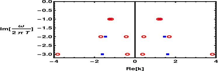
Figure 5: The plot of real part (right panel) and imaginary part (left panel) of $k$ vs $\text{Im}[\frac{\omega}{2\pi T}]$ for $p=2$, $m^{2}=-2$, $\phi(r_{0})=1.1$, $\alpha^{\prime}=0$ (solid rectangle) and $\alpha^{\prime}=0.01$ (open circle).

Here we have compared the position of pole skipping points of $\phi^{2}$ interaction with the absence of interaction ($\alpha^{\prime}=0$) in Figure 5. The real and imaginary parts of $k$ have been separately plotted against $\omega/2i\pi T$. In both cases, the real and imaginary parts are almost equal to each other in each mode. For each part, the values have mirror symmetry with respect to the $\text{Re}[k]=\text{Im}[k]=0$ axes. The shift due to interaction is very hard to identify in $k_{1}$. For $k_{2}$ and $k_{3}$ on the other hand, one observes a measurable amount of shift. It has been depicted in above Figure 5. Without interaction, in each of these three modes, only four real numbers make four different complex $k$ (having equal absolute values of real and imaginary part). With interaction, the same happened for $k_{1}$. But for $k_{2}$ and $k_{3}$ eight real numbers makes four complex values of $k$.

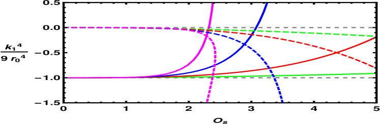
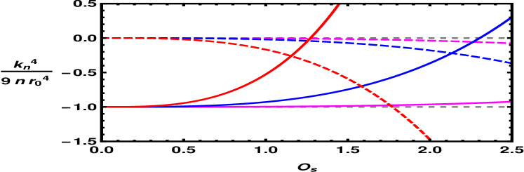
Figure 6: Left: The plot of real (solid line) and imaginary (dashed line) parts of $\frac{k_{1}^{4}}{9r_{0}^{4}}$ vs $\mathcal{O}_{s}$ for different order $\eta$. For $\alpha^{\prime}=0.001$, $m^{2}=-2$, $p=2$ (green color), $p=3$ (red color), $p=4$ (blue color) and $p=5$ (magenta color). Right: The plot of real (solid line) and imaginary (dashed line) parts of $\frac{k_{n}^{4}}{9nr_{0}^{4}}$ vs $\mathcal{O}_{s}$ for different pole-skipping points. For $\alpha^{\prime}=0.001$, $m^{2}=-2$, $p=3$, $n=1$ (magenta color), $n=2$ (blue color) and $n=3$ (red color).

Again we have numerically shown the variation of $k$ with the source $\mathcal{O}_{s}$ of the scalar in Figure 6. At the left plot of this figure, we have plotted the real and imaginary parts of $k^{4}/(9r_{0}^{4})$ against the scalar source. Here we have evaluated the ratio of our result with the result of pure AdS-Schwarzchild. This ratio has no explicit $r_{0}$ dependent. It depends on scalar mass, interaction order, and scalar value on the horizon. For $\alpha^{\prime}=0.001$, $m^{2}=-2$, and for different $p$ the ratio has been evaluated. When the source is off, the imaginary part of the mentioned ratio is zero, whereas the real part is $-1$. Which is consistent with the case without interaction. The imaginary part in $k^{4}$ is contributed only from the interaction. As we have seen at the small value source is linearly proportional to $\phi(r_{0})$, so, $\phi(r_{0})$ also goes to zero as the source becomes zero and thus vanishes the correction term in (4.9). For $p=2,\,3,\,4\,\&\,5$ we have found the same behaviour as $\mathcal{O}_{s}\to 0$. Now if the source is turned on and increased gradually, as long as the source is small enough, both the imaginary and real parts change slowly. However, as $p$ increases the rate of change also increases. The reason is clear from the presence of $\phi(r_{0})^{p}$ factor in the correction terms. During this change the imaginary part of the ratio $k_{1}^{4}/9r_{0}^{4}$ shifts from $0$ towards $-1$ and the real part changes in the exact opposite direction. Therefore the absolute value of the real (imaginary) part decreases (increases). Thus at some point on $\mathcal{O}_{s}$, real and imaginary lines cross each other where their value is exactly equal and lie in between $0$ and $1$. Again after a certain amount of increase in the source, the real part crosses the horizontal axis. At that value $\mathcal{O}_{s}$, $k_{1}^{4}$ becomes a completely imaginary number. These two cross-over points highly depend on $p$, in the given plot, the $p=3$ plot has made the first cross-over whereas the $p=1$ plot has made the last cross-over. As the source value increases further the real (imaginary) values become more and more positive (negative). Since we are interested in the perturbative effect, we will not consider those high values of $k_{1}^{4}$. At the right panel of the same figure, we have plotted the ratio $k_{n}^{4}/(9nr_{0}^{4})$ where $n=1,\,2\,\&\,3$. Here interaction order is fixed at $\phi^{3}$. We have noticed that the behaviour of the real and imaginary parts of the ratio is almost identical to the left panel. We have found the two cross-overs for each of the three modes of $k$. At these cross-over points, the behaviour of $k_{n}^{2}$ is completely identical to before. For the lowest order pole-skipping, $k_{1}$, the cross-over happened at the highest $\mathcal{O}_{s}$ value, and the cross-over points come closer to $\mathcal{O}_{s}=0$ as the order of pole-skipping increases. Therefore the order of interaction and the order of the pole-skipping affect $k$ in the same way. Mainly the location of the cross-over points is almost identically affected by these two parameters. However, the cross-over points can be found analytically from (4.9)-(4.11). For example, the real and imaginary parts of $k_{1}^{4}$ are

$$\text{Re}[k_{1}^{4}]=-9r_{0}^{4}\left(1-\frac{1}{3}\alpha^{\prime}p^{2}m^{4}\phi(r_{0})^{p}\right),\hskip 56.9055pt\text{Im}[k_{1}^{4}]=3\alpha^{\prime}pm^{2}r_{0}^{4}\left(12+pm^{2}\right)\phi(r_{0})^{p}$$

The first cross-over happens at the value of $\mathcal{O}_{s}$ corresponding to $\phi(r_{0})=\left(-4\alpha^{\prime}m^{2}p\right)^{-1/p}$ where the real and imaginary part of $k_{1}^{4}$ are equal to each other. The (second) cross-over on the $\mathcal{O}_{s}$ axis occurs for $\phi(r_{0})=\left(\frac{3}{\alpha^{\prime}p^{2}m^{4}}\right)^{1/p}$. Here $k_{1}^{4}$ is completely imaginary $9ir_{0}^{4}\left(\frac{12}{m^{2}p}+1\right)$. The first cross-over occurs only if $m^{2}<0$. For a moment if we assume that $m^{2}>0$, then there is only the second cross-over where the $k_{1}^{4}$ becomes completely imaginary.

5 Analysis of chaos

5.1 From $vv$ component of linearised Einstein equation

From the shock wave analysis, it is found that the exponential factor of OTOC can be directly observed from the $\delta E_{00}$ component of the linearized Einstein equation in the in-going Eddington-Finkelstein co-ordinate. In the discussed background (2.7), the information about OTOC can be obtained from the $vv$ component of the equation (2.5). Considering the metric perturbation coupled with the $vv$ component of the metric (which are actually the perturbations associated with the sound mode) one can write the $\delta E_{vv}$ at $r=r_{0}$ as follows.

$$\delta g_{vv}(r_{0})\left(k^{2}-2ir_{0}\omega\right)+k\delta g_{vx}(r_{0})\left(2\omega-3ir_{0}\right)=0$$ (5.1)

Since it is well-known that at the special points $(\omega_{*},\,k_{*})$, we have no constraint on the perturbed metric components at $r=r_{0}$ Blake:2018leo . Therefore in the above equation the coefficients of $\delta g_{vv}(r_{0})$ and $\delta g_{vx}(r_{0})$ have to zero. Thus we have

$$\omega_{*}=\frac{3ir_{0}}{2}=2\pi iT,\hskip 28.45274ptk_{*}^{2}=-3r_{0}^{2}$$ (5.2)

This $(\omega_{*},k_{*})$ is the zeroth order pole-skipping point which is connected to the Lyapunov exponent and butterfly velocity as shown in (1.2). In our model, we get, $\lambda_{L}=2\pi T$ and $v_{B}=\frac{\sqrt{3}}{2}$, which is the exact resultBlake:2019otz as in the case of background where the coupling term is not present in the action.

5.2 From the master equation

In the last section, where we have discussed the pole-skipping of the sound mode perturbation, we took the condition that $3k^{2}\neq 4\omega^{2}$. Because we have seen at the horizon the differential equation (4.8) encounters a singularity. Here we will discuss that issue. From past works Blake:2019otz ; Wu:2019esr , we have seen that $3k^{2}=4\omega^{2}$ had come with a new set of points $(\omega,\,k)$ in $\text{Im}[\omega]>0$ plane which was actually related to the chaos parameters. In our case, we can re-arrange the master equation (4.8) as

$$\mathcal{Z}_{so}^{\prime\prime}(r)+P(r)\mathcal{Z}_{so}^{\prime}(r)+Q(r)\mathcal{Z}_{so}(r)=0$$ (5.3)

In this equation, the denominators of both $P(r)$ and $Q(r)$ has a multiplicative factor of $\left(3+f(r)\right)k^{2}-4\omega^{2}$ which reduces to $3k^{2}-4\omega^{2}$ at $r=r_{0}$. So to get the regular solution of (5.3) at $r=r_{0}$, we must impose an extra condition on $\omega$ or $k$. Here we will find it.

First we put $k=\frac{2}{\sqrt{3}}\omega$ in (5.3) and expand it around $r=r_{0}$. We find that $P(r)$ and $Q(r)$ process the first and second order pole at $r=r_{0}$.

$$P(r) = \frac{P_{-1}}{(r-r_{0})}+\mathcal{O}\left((r-r_{0})^{0}\right),\hskip 36.98866ptP_{-1}=-1-\frac{2i\omega}{3r_{0}}-\frac{144\alpha^{\prime}ir_{0}\omega\zeta^{\prime}(r_{0})}{3r_{0}-2i\omega}$$

$$Q(r) = \frac{Q_{-2}}{(r-r_{0})^{2}}+\mathcal{O}\left((r-r_{0})^{-1}\right),\hskip 22.76228ptQ_{-2}=1+\frac{2i\omega}{3r_{0}}+\frac{4i\alpha^{\prime}\omega(27r_{0}^{2}+12ir_{0}\omega+4\omega^{2})\zeta^{\prime}(r_{0})}{r_{0}(3r_{0}-2i\omega)}$$

Therefore $r=r_{0}$ is a regular singular point for the differential equation (5.3). Now, suppose $\mathcal{Z}_{so}$ has a series solution near the singular point given as

$$\mathcal{Z}_{so}=(r-r_{0})^{l}\sum_{n\in[0,\mathbb{Z}^{+})}\mathcal{Z}_{n}(r-r_{0})^{n}$$ (5.4)

The only condition which makes this solution regular at the horizon is $l=0,1,2,\cdots$. Therefore the first recursion relation coming from (5.3) is

$$l^{2}+l\left(P_{-1}-1\right)+Q_{-2}=0.$$ (5.5)

This gives two roots (say, $l_{1}$ and $l_{2}$) in the following form.

$$l_{1} = 1-6\alpha^{\prime}(3r_{0}-2i\omega)\zeta^{\prime}(r_{0})$$

$$l_{2} = 1+\frac{2i\omega}{3r_{0}}+6\alpha^{\prime}\frac{(3r_{0}+2i\omega)^{2}}{3r_{0}-2i\omega}\zeta^{\prime}(r_{0})$$

So for arbitrary interaction, the only possible integer roots are $l_{1}=1$ and $l_{2}=0$. This gives only two values of $\omega$ as $\pm\frac{3}{2}ir_{0}$. Therefore we get the same values of the chaos parameters as we have already found in the last subsection.

6 Discussions

Here in this article, we have studied the pole-skipping phenomena in non-extremal gravity theory in presence of the Gauss-Bonnet-scalar interaction. We have considered a four-dimensional Schwarzchild-AdS black hole solution as the holographic bulk theory. On the boundary, we have a finite temperature conformal theory. The interaction is sourced by an operator of dimension $\Delta$ of the boundary theory, which is dual to the scalar field $\phi$ in the bulk. In the Einstein action, the interaction term is added perturbatively (2.1). In the perturbative approximation, this external scalar source has no effect on the original bulk solution but made a nontrivial contribution in the linearised field equations (2.5). We have found that $k$ of the pole-skipping points ($\omega,\,k$) corresponding to the scalar field and metric perturbation have been affected by the external scalar source $\mathcal{O}_{s}$. Whereas, $\omega$ remains unchanged.

Unlike the unperturbed model, the minimally coupled scalar $\phi$ has contained both real and imaginary $k$ in the pole-skipping points. As the source is increased, the points of the imaginary $k$ plane have moved into the real $k$ plane. We have presented these facts pictorially in Figure 2. In Schwarzchild-AdS₄ without external effect Blake:2019otz , $k$ is always real in the shear mode. Here we have found that the shear mode $k$ has the possibility to have both real and imaginary values depending on the effect of the scalar source. We have analytically found the effect of the interaction on the first three poles located at $\omega_{n}=-2in\pi T$ and corresponding $k\sim T$ which are given in (4.3), (4.4) $\&$ (4.5). The first order pole-point $k_{1}^{2}$ is always greater than $3r_{0}^{2}$ for $\zeta=\phi,\,\phi^{2},\,\phi^{3}\,\&\,\phi^{4}$ and has decreased for other higher powers of $\phi$. However, for the second and other higher orders of pole-skipping, $k^{2}$ has always decreased with the increasing source for all positive integer powers of $\phi$ in $\zeta(\phi)$. These have been shown in Figure 3. Here, the increase (or decrease) of real $k$ implies a slow (or fast) rate of momentum transportation in shear mode and the imaginary $k$ means the exponential decay of the momentum density. As a result, when positive $k_{1}^{2}$ has increased with the increasing source $\mathcal{O}_{s}$, the mobility of the corresponding modes has decreased. Thus the decreasing mobility has decreased the value of diffusion coefficient $\mathcal{D}_{s}$. In Figure 4, we have presented this consistent behaviour of diffusion coefficient. At $\mathcal{O}_{s}\to 0$, $k_{1}^{2}$ is at a minimum value, and therefore, momentum flow is maximum which has given the maximum value of $\mathcal{D}_{s}$. So, due to the effect of the external source, the flow of momentum in shear mode has decreased for $p\leq 4$, otherwise, it has increased.

In the sound mode, the first three pole-skipping points have been derived from the master equation as $\omega_{n}=-2\pi inT$ and corresponding $k_{n}\sim T$ is given in (4.9), (4.10) $\&$ (4.11). In the non-perturbative case where either $\alpha^{\prime}\to 0$ or $\mathcal{O}_{s}\to 0$, our results have reduced into the pole-skipping points of pure Schwarzchild-AdS₄ background Blake:2019otz , i.e, $k_{n}^{4}=-9nr_{0}^{4}$. It gives a complex value (of equal real and imaginary parts) of $k$. As the source is turned on, we have found that an imaginary part has been added with the negative real part of $k^{4}$. It means the real and imaginary part of $k$ is no more equal. We have shown all of these in Figure 6. However, from the OTOC calculation in the last section, we have found the Lyapunov exponent $\lambda=-i\omega=2\pi T$ and the butterfly velocity $v_{b}=\frac{\sqrt{3}}{2}$ where $\omega_{*}=2i\pi T$ and $k_{*}=\pm\frac{4}{\sqrt{3}}i\pi T$. These results have been further verified with a different approach by analyzing the power series solution of the sound mode master equation near the horizon. Therefore ($\omega_{*},\,k_{*}$) is considered as the lowest order pole-skipping point in sound mode instead of ($\omega_{1},\,k_{1}$). So the pole-skipping points of sound mode are ($\omega_{*},\,k_{*}$), ($\omega_{1},\,k_{1}$), ($\omega_{2},\,k_{2}$), ($\omega_{3},\,k_{3}$) and so on. The pole-skipping points $(\omega,\,k)$ describe the flow of energy density. Here $k$ has both the real and imaginary parts. It signifies that the real part is associated with the flow of the energy density in longitudinal mode whereas the imaginary part of $k$ is related to the exponential decay of the energy density. Therefore with the effect of interaction, when the energy density diffusion has increased the exponential decay has decreased and vice-versa. It would be interesting to study these flows and decays quantitatively.

However, we have found some non-trivial effects of the interaction on the sound mode and shear mode. We have not found any effect on the chaotic behaviour. The reason is mainly the perturbative approach to the interaction term. If one considers the backreaction of the interaction, the Lyapunov exponent and the butterfly velocity are expected to be affected by the interaction. With backreaction, one can expect $k_{*}$ and $k_{1}$ to be equal in the sound mode.

Appendix A Coefficient of Master Equation: Shear Channel

Three coefficients of the master equation can be written in the linear order of the perturbation parameter $\alpha^{\prime}$

$$\mathcal{M}_{sh}(r) = \mathcal{M}_{sh}^{(0)}+\alpha^{\prime}\mathcal{M}_{sh}^{(1)}+\mathcal{O}(\alpha^{\prime 2})$$

$$\mathcal{P}_{sh}(r) = \mathcal{P}_{sh}^{(0)}+\alpha^{\prime}\mathcal{P}_{sh}^{(1)}+\mathcal{O}(\alpha^{\prime 2})$$

$$\mathcal{Q}_{sh}(r) = \mathcal{Q}_{sh}^{(0)}+\alpha^{\prime}\mathcal{Q}_{sh}^{(1)}+\mathcal{O}(\alpha^{\prime 2})$$

We have found the above functions as follows.

$$\mathcal{M}_{sh}^{(0)} = r^{2}f(r)$$ (A.1)

$$\mathcal{P}_{sh}^{(0)} = \frac{\omega f(r)\left(5r\omega+2ik^{2}\right)-8k^{2}rf(r)^{2}+\omega^{2}(3r-2i\omega)}{\omega^{2}-k^{2}f(r)}$$ (A.2)

$$\mathcal{Q}_{sh}^{(0)} = \frac{-10k^{2}r^{2}f(r)^{2}+f(r)\left(k^{4}+9ik^{2}r\omega+4r^{2}\omega^{2}\right)+\omega\left(k^{2}(-\omega-3ir)+6r\omega(r-i\omega)\right)}{r^{2}\left(\omega^{2}-k^{2}f(r)\right)}$$

and

$$\mathcal{M}_{sh}^{(1)} = 0$$ (A.4)

$$\mathcal{P}_{sh}^{(1)} = \frac{r^{2}f(r)}{\left(\omega^{2}-k^{2}f(r)\right)^{2}}\left[r\zeta^{\prime\prime}(r)\left(\omega^{2}-k^{2}f(r)\right)\left(f(r)\left(2k^{2}f(r)+\omega^{2}\right)-3\omega^{2}\right)+\zeta^{\prime}(r)\left(f(r)\right.\right.$$ (A.5)

$$\left.\left.\left.(k^{2}f(r)\left(4k^{2}f(r)-6k^{2}-11\omega^{2}\right)+24k^{2}\omega^{2}-2\omega^{4}\right)-9k^{2}\omega^{2}\right)-\omega\mathcal{F}\right]$$

$$\mathcal{Q}_{sh}^{(1)} = \frac{1}{r\left(\omega^{2}-k^{2}f(r)\right)^{2}}\left[r\zeta^{\prime\prime}(r)\left(\omega^{2}-k^{2}f(r)\right)\left(f(r)\left(\omega^{2}\left(4k^{2}-ir\omega\right)-2k^{2}f(r)\left(-3r^{2}f(r)\right.\right.\right.\right.$$ (A.6)

$$+k^{2}+3r^{2}+ir\omega\left.+\omega^{3}(-2\omega+3ir)\right)+\zeta^{\prime}(r)\left(f(r)\left(f(r)\left(-k^{2}f(r)\left(-14k^{2}r^{2}f(r)+3k^{4}\right.\right.\right.\right.$$

$$\left.\left.+4k^{2}r(6r+i\omega)+34r^{2}\omega^{2}\right)+3k^{6}+6k^{4}\left(3r^{2}+ir\omega+\omega^{2}\right)+k^{2}r\omega^{2}(72r+11i\omega)\right.$$

$$\left.\left.\left.+2r^{2}\omega^{4}\right)+\omega^{2}\left(-6k^{4}-3k^{2}\left(18r^{2}+8ir\omega+\omega^{2}\right)+2r\omega(-6r+i\omega)\right)\right)+3\omega^{3}\left(6r^{2}\omega\right.\right.$$

$$\left.\left.\left.+k^{2}(\omega+3ir)\right)\right)+ir\left(2\omega^{2}-f(r)\left(k^{2}-2ir\omega\right)\right)\mathcal{F}\right]$$

where,

$$\mathcal{F} = 6k^{2}r^{2}\omega(f(r)-1)\left[r(f(r)-3)f(r)\zeta^{\prime\prime}(r)-3((f(r)-2)f(r)+3)\zeta^{\prime}(r)\right]^{2}/\left[r\zeta^{\prime\prime}(r)\left(f(r)\left(f(r)\right.\right.\right.$$

$$\left.\left.\left.\left(k^{2}-3ir\omega\right)-3k^{2}+3ir\omega\right)-18ir\omega\right)-3\zeta^{\prime}(r)\left((f(r)-2)f(r)\left(k^{2}-ir\omega\right)+3\left(k^{2}+3ir\omega\right)\right)\right.$$

$$\left.+ir^{3}\omega(f(r)-3)f(r)\zeta^{\prime\prime\prime}(r)\right]$$

Here the $\zeta$ function takes its appropriate form.

Appendix B Coefficient of Master Equation: Sound Channel

Three coefficients of the master equation can be written in the linear order of the perturbation parameter $\alpha^{\prime}$

$$\mathcal{M}_{so}(r) = \mathcal{M}_{so}^{(0)}+\alpha^{\prime}\mathcal{M}_{so}^{(1)}+\mathcal{O}(\alpha^{\prime 2})$$

$$\mathcal{P}_{so}(r) = \mathcal{P}_{so}^{(0)}+\alpha^{\prime}\mathcal{P}_{so}^{(1)}+\mathcal{O}(\alpha^{\prime 2})$$

$$\mathcal{Q}_{so}(r) = \mathcal{Q}_{so}^{(0)}+\alpha^{\prime}\mathcal{Q}_{so}^{(1)}+\mathcal{O}(\alpha^{\prime 2})$$

where,

$$\mathcal{M}_{so}^{(0)} = r^{4}f(r)$$ (B.1)

$$\mathcal{P}_{so}^{(0)} = \frac{r^{2}\left(f(r)\left(11k^{2}rf(r)+2k^{2}(6r-i\omega)-20r\omega^{2}\right)+\left(3k^{2}-4\omega^{2}\right)(3r-2i\omega)\right)}{k^{2}f(r)+3k^{2}-4\omega^{2}}$$ (B.2)

$$\mathcal{Q}_{so}^{(0)} = \frac{1}{k^{2}f(r)+3k^{2}-4\omega^{2}}\left(-f(r)\left(-25k^{2}r^{2}f(r)+k^{4}+12k^{2}r(r+i\omega)+16r^{2}\omega^{2}\right)-3k^{4}\right.$$ (B.3)

$$\left.\hskip 28.45274pt+k^{2}(9r+2i\omega)(3r-2i\omega)-24r\omega^{2}(r-i\omega)\right)$$

$$\mathcal{M}_{so}^{(1)} = 0$$ (B.4)

$$\mathcal{P}_{so}^{(1)} = \frac{r^{2}f(r)}{\left(2ir\omega+k^{2}\right)\left(k^{2}f(r)+3k^{2}-4\omega^{2}\right)^{3}}\left[r^{3}\zeta^{\prime\prime}(r)\left\{f(r)\left(k^{2}f(r)\left(k^{2}f(r)^{2}\left(9k^{4}\right.\right.\right.\right.\right.$$ (B.5)

$$\left.+2k^{2}r(-24r+25i\omega)+64r^{2}\omega^{2}\right)+2f(r)\left(-27k^{6}+6k^{4}\left(24r^{2}-9ir\omega+11\omega^{2}\right)\right.$$

$$\left.+4k^{2}r\omega^{2}(-72r+17i\omega)+128r^{2}\omega^{4}\right)+12\left(3k^{2}-4\omega^{2}\right)\left(2k^{4}+k^{2}\left(-12r^{2}-4ir\omega\right.\right.$$

$$\left.\left.\left.\left.+3\omega^{2}\right)+2r\omega^{2}(8r+3i\omega)\right)\right)+2\left(3k^{2}-2\omega^{2}\right)\left(3k^{2}-4\omega^{2}\right)^{2}\left(k^{2}+2ir\omega\right)\right)-3\left(3k^{2}\right.$$

$$\left.\left.-4\omega^{2}\right)^{3}\left(k^{2}+2ir\omega\right)\right\}+4\zeta^{\prime}(r)\left\{f(r)\left(k^{2}f(r)\left(r^{2}f(r)\left(-k^{2}f(r)\left(5k^{4}+3k^{2}r(-12r\right.\right.\right.\right.\right.$$

$$\left.+7i\omega)+48r^{2}\omega^{2}\right)+9k^{6}+k^{4}\left(-180r^{2}+33ir\omega-26\omega^{2}\right)+4k^{2}r\omega^{2}(96r+5i\omega)$$

$$\left.-192r^{2}\omega^{4}\right)+3k^{8}+4k^{6}\left(36r^{2}+6ir\omega-\omega^{2}\right)+k^{4}r\left(324r^{3}+243ir^{2}\omega-324r\omega^{2}\right.$$

$$\left.\left.-32i\omega^{3}\right)-8k^{2}r^{2}\omega^{2}\left(90r^{2}+81ir\omega-34\omega^{2}\right)+48r^{3}\omega^{4}(8r+9i\omega)\right)+\left(3k^{2}-4\omega^{2}\right)\left(3k^{8}\right.$$

$$-k^{6}\left(63r^{2}+4\omega^{2}\right)-k^{4}r\left(108r^{3}+171ir^{2}\omega-126r\omega^{2}+8i\omega^{3}\right)+8k^{2}r^{2}\omega^{2}\left(18r^{2}\right.$$

$$\left.\left.\left.\left.\left.+27ir\omega-\omega^{2}\right)-16ir^{3}\omega^{5}\right)\right)+9k^{2}r^{2}\left(3k^{2}-4\omega^{2}\right)^{2}\left(k^{2}+2ir\omega\right)\right\}\right]$$

$$\mathcal{Q}_{so}^{(1)} = -\frac{1}{r\left(2ir\omega+k^{2}\right)\left(f(r)k^{2}+3k^{2}-4\omega^{2}\right)^{3}}\left[\left\{\omega(3r+2i\omega)\left(2r\omega-ik^{2}\right)\left(3k^{2}-4\omega^{2}\right)^{3}\right.\right.$$ (B.6)

$$+f(r)\left(f(r)\left(f(r)\left(-3k^{8}+18\left(-19r^{2}-2i\omega r+\omega^{2}\right)k^{6}+4r(3r-i\omega)\left(108r^{2}+99i\omega r\right.\right.\right.\right.$$

$$\left.-26\omega^{2}\right)k^{4}-8r^{2}\omega^{2}\left(360r^{2}+234i\omega r-85\omega^{2}\right)k^{2}+32r^{3}\omega^{4}(48r+35i\omega)+f(r)\left(3k^{8}\right.$$

$$+r(180r+23i\omega)k^{6}-2r^{2}\left(576r^{2}-108i\omega r+257\omega^{2}\right)k^{4}+64r^{3}\omega^{2}(30r-i\omega)k^{2}$$

$$\left.\left.-r^{2}\left(43k^{4}+6r(41i\omega-40r)k^{2}+320r^{2}\omega^{2}\right)f(r)k^{2}-512r^{4}\omega^{4}\right)\right)-\left(3k^{2}-4\omega^{2}\right)\left(9k^{6}\right.$$

$$\left.\left.\left.+6\left(18r^{2}+3i\omega r-7\omega^{2}\right)k^{4}+8ir\omega\left(45r^{2}+42i\omega r-11\omega^{2}\right)k^{2}+8r^{2}\omega^{3}(\omega-60ir)\right)\right)k^{2}\right.$$

$$\left.\left.+\left(k^{2}+2ir\omega\right)\left(3k^{2}-4\omega^{2}\right)^{2}\left(3k^{4}+\left(9r^{2}-18i\omega r+14\omega^{2}\right)k^{2}-4ir\omega^{3}\right)\right)\right\}\zeta^{\prime\prime}(r)r^{3}$$

$$+\left\{\left(k^{2}+2ir\omega\right)\left(3k^{6}+2\omega(-3ir-2\omega)k^{4}-6r^{2}\left(9r^{2}+6i\omega r-2\omega^{2}\right)k^{2}\right.\right.$$

$$\left.+72r^{4}\omega^{2}\right)\left(3k^{2}-4\omega^{2}\right)^{2}+f(r)\left(2\left(3k^{2}-4\omega^{2}\right)\left(3k^{10}+\left(63r^{2}+18i\omega r-4\omega^{2}\right)k^{8}\right.\right.$$

$$\left.-r\left(189r^{3}+18i\omega r^{2}+66\omega^{2}r+28i\omega^{3}\right)k^{6}+2r^{2}\omega\left(-297ir^{3}+315\omega r^{2}+6i\omega^{2}r+28\omega^{3}\right)k^{4}\right.$$

$$\left.+8ir^{3}\omega^{3}\left(63r^{2}+18i\omega r+4\omega^{2}\right)k^{2}+32r^{4}\omega^{5}(6ir+\omega)\right)+f(r)\left(3k^{12}+\left(-90r^{2}+36i\omega r\right.\right.$$

$$\left.-4\omega^{2}\right)k^{10}+12r\left(171r^{3}+63i\omega r^{2}+24\omega^{2}r-4i\omega^{3}\right)k^{8}+4r^{2}\left(972r^{4}+1971i\omega r^{3}\right.$$

$$\left.-1863\omega^{2}r^{2}-186i\omega^{3}r-32\omega^{4}\right)k^{6}-32r^{3}\omega^{2}\left(270r^{3}+531i\omega r^{2}-243\omega^{2}r-i\omega^{3}\right)k^{4}$$

$$+64r^{4}\omega^{4}\left(72r^{2}+132i\omega r-13\omega^{2}\right)k^{2}+2r^{2}f(r)\left(3\left(-15k^{8}-2\left(186r^{2}+37i\omega r-9\omega^{2}\right)k^{6}\right.\right.$$

$$\left.+2r\left(-396r^{3}-417i\omega r^{2}+339\omega^{2}r+50i\omega^{3}\right)k^{4}+8r^{2}\omega^{2}\left(180r^{2}+232i\omega r-73\omega^{2}\right)k^{2}\right.$$

$$\left.-64r^{3}(8r+13i\omega)\omega^{4}\right)+f(r)\left(-3k^{8}+r(21r-20i\omega)k^{6}+2r^{2}\left(684r^{2}-24i\omega r+43\omega^{2}\right)k^{4}\right.$$

$$\left.-8r^{3}(300r+91i\omega)\omega^{2}k^{2}+r^{2}\left(47k^{4}+12r(17i\omega-30r)k^{2}+480r^{2}\omega^{2}\right)f(r)k^{2}\right.$$

$$\hskip 28.45274pt\left.\left.\left.\left.\left.\left.+768r^{4}\omega^{4}\right)\right)k^{2}+256ir^{5}\omega^{7}\right)\right)\right\}\zeta^{\prime}(r)\right]$$

- (1) Y. Gu, X. L. Qi and D. Stanford, “Local criticality, diffusion and chaos in generalized Sachdev-Ye-Kitaev models,” JHEP 05 (2017), 125 doi:10.1007/JHEP05(2017)125 [arXiv:1609.07832 [hep-th]].
- (2) A. A. Patel and S. Sachdev, “Quantum chaos on a critical Fermi surface,” Proc. Nat. Acad. Sci. 114 (2017), 1844-1849 doi:10.1073/pnas.1618185114 [arXiv:1611.00003 [cond-mat.str-el]].
- (3) S. Grozdanov, K. Schalm and V. Scopelliti, “Kinetic theory for classical and quantum many-body chaos,” Phys. Rev. E 99 (2019) no.1, 012206 doi:10.1103/PhysRevE.99.012206 [arXiv:1804.09182 [hep-th]].
- (4) J. M. Maldacena, “The Large N limit of superconformal field theories and supergravity,” Adv. Theor. Math. Phys. 2 (1998), 231-252 doi:10.1023/A:1026654312961 [arXiv:hep-th/9711200 [hep-th]].
- (5) O. Aharony, S. S. Gubser, J. M. Maldacena, H. Ooguri and Y. Oz, “Large N field theories, string theory and gravity,” Phys. Rept. 323 (2000), 183-386 doi:10.1016/S0370-1573(99)00083-6 [arXiv:hep-th/9905111 [hep-th]].
- (6) M. Blake, H. Lee and H. Liu, “A quantum hydrodynamical description for scrambling and many-body chaos,” JHEP 10 (2018), 127 doi:10.1007/JHEP10(2018)127 [arXiv:1801.00010 [hep-th]].
- (7) M. Blake, R. A. Davison, S. Grozdanov and H. Liu, “Many-body chaos and energy dynamics in holography,” JHEP 10 (2018), 035 doi:10.1007/JHEP10(2018)035 [arXiv:1809.01169 [hep-th]].
- (8) M. Blake, R. A. Davison and D. Vegh, “Horizon constraints on holographic Green’s functions,” JHEP 01 (2020), 077 doi:10.1007/JHEP01(2020)077 [arXiv:1904.12883 [hep-th]].
- (9) M. Blake and R. A. Davison, “Chaos and pole-skipping in rotating black holes,” JHEP 01 (2022), 013 doi:10.1007/JHEP01(2022)013 [arXiv:2111.11093 [hep-th]].
- (10) S. Grozdanov, K. Schalm and V. Scopelliti, “Black hole scrambling from hydrodynamics,” Phys. Rev. Lett. 120 (2018) no.23, 231601 doi:10.1103/PhysRevLett.120.231601 [arXiv:1710.00921 [hep-th]].
- (11) S. H. Shenker and D. Stanford, “Stringy effects in scrambling,” JHEP 05 (2015), 132 doi:10.1007/JHEP05(2015)132 [arXiv:1412.6087 [hep-th]].
- (12) M. Natsuume and T. Okamura, “Nonuniqueness of Green’s functions at special points,” JHEP 12 (2019), 139 doi:10.1007/JHEP12(2019)139 [arXiv:1905.12015 [hep-th]].
- (13) M. Natsuume and T. Okamura, “Holographic chaos, pole-skipping, and regularity,” PTEP 2020 (2020) no.1, 013B07 doi:10.1093/ptep/ptz155 [arXiv:1905.12014 [hep-th]].
- (14) Y. Ahn, V. Jahnke, H. S. Jeong and K. Y. Kim, “Scrambling in Hyperbolic Black Holes: shock waves and pole-skipping,” JHEP 10 (2019), 257 doi:10.1007/JHEP10(2019)257 [arXiv:1907.08030 [hep-th]].
- (15) Y. Ahn, V. Jahnke, H. S. Jeong, K. Y. Kim, K. S. Lee and M. Nishida, “Pole-skipping of scalar and vector fields in hyperbolic space: conformal blocks and holography,” JHEP 09 (2020), 111 doi:10.1007/JHEP09(2020)111 [arXiv:2006.00974 [hep-th]].
- (16) M. A. G. Amano, M. Blake, C. Cartwright, M. Kaminski and A. P. Thompson, “Chaos and pole-skipping in a simply spinning plasma,” [arXiv:2211.00016 [hep-th]].
- (17) K. Sil, “Pole skipping and chaos in anisotropic plasma: a holographic study,” JHEP 03 (2021), 232 doi:10.1007/JHEP03(2021)232 [arXiv:2012.07710 [hep-th]].
- (18) M. Atashi and K. Bitaghsir Fadafan, “Holographic pole – skipping of flavor branes,” JHAP 3 (2022) no.1, 39-46 doi:10.22128/jhap.2022.519.1020
- (19) H. Yuan and X. H. Ge, “Pole-skipping and hydrodynamic analysis in Lifshitz, AdS2 and Rindler geometries,” JHEP 06 (2021), 165 doi:10.1007/JHEP06(2021)165 [arXiv:2012.15396 [hep-th]].
- (20) K. Y. Kim, K. S. Lee and M. Nishida, “Holographic scalar and vector exchange in OTOCs and pole-skipping phenomena,” JHEP 04 (2021), 092 [erratum: JHEP 04 (2021), 229] doi:10.1007/JHEP04(2021)092 [arXiv:2011.13716 [hep-th]].
- (21) C. Choi, M. Mezei and G. Sárosi, “Pole skipping away from maximal chaos,” doi:10.1007/JHEP02(2021)207 [arXiv:2010.08558 [hep-th]].
- (22) N. Ceplak, K. Ramdial and D. Vegh, “Fermionic pole-skipping in holography,” JHEP 07 (2020), 203 doi:10.1007/JHEP07(2020)203 [arXiv:1910.02975 [hep-th]].
- (23) M. Natsuume and T. Okamura, “Pole-skipping with finite-coupling corrections,” Phys. Rev. D 100 (2019) no.12, 126012 doi:10.1103/PhysRevD.100.126012 [arXiv:1909.09168 [hep-th]].
- (24) X. Wu, “Higher curvature corrections to pole-skipping,” JHEP 12 (2019), 140 doi:10.1007/JHEP12(2019)140 [arXiv:1909.10223 [hep-th]].
- (25) M. Natsuume and T. Okamura, “Pole-skipping and zero temperature,” Phys. Rev. D 103 (2021) no.6, 066017 doi:10.1103/PhysRevD.103.066017 [arXiv:2011.10093 [hep-th]].
- (26) S. Grozdanov, “On the connection between hydrodynamics and quantum chaos in holographic theories with stringy corrections,” JHEP 01 (2019), 048 doi:10.1007/JHEP01(2019)048 [arXiv:1811.09641 [hep-th]].
- (27) S. Grozdanov, P. K. Kovtun, A. O. Starinets and P. Tadić, “The complex life of hydrodynamic modes,” JHEP 11 (2019), 097 doi:10.1007/JHEP11(2019)097 [arXiv:1904.12862 [hep-th]].
- (28) W. Li, S. Lin and J. Mei, “Thermal diffusion and quantum chaos in neutral magnetized plasma,” Phys. Rev. D 100 (2019) no.4, 046012 doi:10.1103/PhysRevD.100.046012 [arXiv:1905.07684 [hep-th]].
- (29) N. Abbasi and S. Tahery, “Complexified quasinormal modes and the pole-skipping in a holographic system at finite chemical potential,” JHEP 10 (2020), 076 doi:10.1007/JHEP10(2020)076 [arXiv:2007.10024 [hep-th]].
- (30) N. Abbasi and M. Kaminski, “Constraints on quasinormal modes and bounds for critical points from pole-skipping,” JHEP 03 (2021), 265 doi:10.1007/JHEP03(2021)265 [arXiv:2012.15820 [hep-th]].
- (31) N. Ceplak and D. Vegh, “Pole-skipping and Rarita-Schwinger fields,” Phys. Rev. D 103 (2021) no.10, 106009 doi:10.1103/PhysRevD.103.106009 [arXiv:2101.01490 [hep-th]].
- (32) J. Maldacena, S. H. Shenker and D. Stanford, “A bound on chaos,” JHEP 08 (2016), 106 doi:10.1007/JHEP08(2016)106 [arXiv:1503.01409 [hep-th]].
- (33) S. Chakrabarti, D. Maity and W. Wahlang, “Probing the Holographic Fermi Arc with scalar field: Numerical and analytical study,” JHEP 07 (2019), 037 doi:10.1007/JHEP07(2019)037 [arXiv:1902.08826 [hep-th]].
- (34) K. B. Huh, H. S. Jeong, K. Y. Kim and Y. W. Sun, “Upper bound of the charge diffusion constant in holography,” JHEP 07 (2022), 013 doi:10.1007/JHEP07(2022)013 [arXiv:2111.07515 [hep-th]].
- (35) T. Hartman, S. A. Hartnoll and R. Mahajan, “Upper Bound on Diffusivity,” Phys. Rev. Lett. 119 (2017) no.14, 141601 doi:10.1103/PhysRevLett.119.141601 [arXiv:1706.00019 [hep-th]].
- (36) P. Kovtun, D. T. Son and A. O. Starinets, “Holography and hydrodynamics: Diffusion on stretched horizons,” JHEP 10 (2003), 064 doi:10.1088/1126-6708/2003/10/064 [arXiv:hep-th/0309213 [hep-th]].