Maintaining Triconnected Components under Node Expansion

Abstract

SPQR-trees are a central component of graph drawing and are also important in many further areas of computer science. From their inception onwards, they have always had a strong relation to dynamic algorithms maintaining information, e.g., on planarity and triconnectivity, under edge insertion and, later on, also deletion. In this paper, we focus on a special kind of dynamic update, the expansion of vertices into arbitrary biconnected graphs, while maintaining the SPQR-tree and further information. This will also allow us to efficiently merge two SPQR-trees by identifying the edges incident to two vertices with each other. We do this working along an axiomatic definition lifting the SPQR-tree to a stand-alone data structure that can be modified independently from the graph it might have been derived from. Making changes to this structure, we can now observe how the graph represented by the SPQR-tree changes, instead of having to reason which updates to the SPQR-tree are necessary after a change to the represented graph.

Using efficient expansions and merges allows us to improve the runtime of the Synchronized Planarity algorithm by Bläsius et al. [8] from $O(m^{2})$ to $O(m\cdot\Delta)$, where $\Delta$ is the maximum pipe degree. This also reduces the time for solving several constrained planarity problems, e.g. for Clustered Planarity from $O((n+d)^{2})$ to $O(n+d\cdot\Delta)$, where $d$ is the total number of crossings between cluster borders and edges and $\Delta$ is the maximum number of edge crossings on a single cluster border.

1 Introduction

The SPQR-tree is a data structure that represents the decomposition of a graph at its separation pairs, that is the pairs of vertices whose removal disconnects the graph. The components obtained by this decomposition are called skeletons. SPQR-trees form a central component of many graph visualization techniques and are used for, e.g., planarity testing and variations thereof [13, 19, 29, 31, 39] and for computing embeddings and layouts [3, 7, 11, 20, 28, 42]; see [37] for a survey of graph drawing applications. Outside of graph visualization they are used in the context of, e.g., minimum spanning trees [6, 17], triangulations [5], and crossing optimization [28, 42]. They also have multiple applications outside of graph theory and even computer science, e.g. for creating integrated circuits [14, 44], business processes modelling [40], electrical engineering [24], theoretical physics [41] and genomics [22].

Initially, SPQR-trees were devised by Di Battista and Tamassia for incremental planarity testing [16, 19]. As such, even in their initial form, SPQR-trees already allowed dynamic updates in the form of edge addition. Their use was quickly expanded to other on-line problems [18, 17]. In addition to the applications mentioned above, this also sparked a series of further papers improving the runtime of the incremental data structure [38, 39, 43] and also extending it to be fully-dynamic, i.e., allowing insertion and deletion of vertices and edges, in $O(\sqrt{n})$ time [21, 27], where $n$ is the number of vertices in the graph. Recently, Holm and Rotenberg described a fully-dynamic algorithm for maintaining planarity and triconnectivity information in $O(\log^{3}n)$ time per operation [31, 32] (see also there for a short history on dynamic SPQR-tree algorithms).

In this paper, we consider an incremental setting where we allow a single operation that expands a vertex $v$ into an arbitrary biconnected graph $G_{\nu}$. Using the approach of Holm and Rotenberg [31], this takes $O((\deg(v)+|G_{\nu}|)\cdot\log^{3}n)$ time by first removing $v$ and its incident edges and then incrementally inserting $G_{\nu}$. We improve this to $O(\deg(v)+|G_{\nu}|)$ using an algorithm that is much simpler and thus also more likely to improve performance in practice. In addition, our approach also allows to efficiently merge two SPQR-trees as follows. Given two biconnected graphs $G_{1},G_{2}$ containing vertices $v_{1},v_{2}$, respectively, together with a bijection between their incident edges, we construct a new graph $G$ by replacing $v_{1}$ with $G_{2}-v_{2}$ in $G_{1}$, identifying edges using the given bijection. Given the SPQR-trees of $G_{1}$ and $G_{2}$, we show that the SPQR-tree of $G$ can be found in $O(\deg(v_{1}))$ time. More specifically, we present a data structure that supports the following operations: ${\texttt{In\-sert}\-\texttt{Graph}_{\texttt{SPQR}}}$ expands a single vertex in time linear in the size of the expanded subgraph, ${\texttt{Merge}_{\texttt{SPQR}}}$ merges two SPQR-trees in time linear in the degree of the replaced vertices, IsPlanar indicates whether the currently represented graph is planar in constant time, and Rotation yields one of the two possible planar rotations of a vertex in a triconnected skeleton in constant time. Furthermore, our data structure can be adapted to yield consistent planar embeddings for all triconnected skeletons and to test for the existence of three distinct paths between two arbitrary vertices with an additional factor of $\alpha(n)$ for all operations, where $\alpha$ is the inverse Ackermann function.

Problem	Running Times
	before [8]	using [8]	with this paper
Atomic Embeddability / Synchronized Planarity	$O(m^{8})$ [26]	$O(m^{2})$	$O(m\cdot\Delta)$
ClusterPlanarity	$O((n+d)^{8})$ [26]	$O((n+d)^{2})$	$O(n+d\cdot\Delta)$
Connected SEFE	$O(n^{16})$ [26]	$O(n^{2})$	$O(n\cdot\Delta)$
	bicon: $O(n^{2})$ [10]
Partially PQ-Constrained Planarity	bicon: $O(m)$ [10]	$O(m^{2})$	$O(m\cdot\Delta)$
Row-Column Independent NodeTrix Planarity	bicon: $O(n^{2})$ [35]	$O(n^{2})$	$O(n\cdot\Delta)$
Strip Planarity	$O(n^{8})$ [4, 26]	$O(n^{2})$	$O(n\cdot\Delta)$
	fixed emb: poly [4]

Table 1: The best known running times for various constrained planarity problems before Synchronized Planarity [8] was published; using it as described in [8]; and using it together with the speed-up from this paper. Running times prefixed with “bicon” only apply for certain problem instances which expose some form of biconnectivity. The variables $n$ and $m$ refer to the number of vertices and edges of the problem instance, respectively. The variable $d$ refers to the number of edge-cluster boundary crossings in Clustered Planarity instances, while $\Delta$ refers to the maximum pipe degree in the corresponding Synchronized Planarity instances. This is bounded by the maximum number of edges crossing a single cluster border or the maximum vertex degree in the input instance, depending on the problem.

The main idea of our approach is that the subtree of the SPQR-tree affected by expanding a vertex $v$ has size linear in the degree of $v$, but may contain arbitrarily large skeletons. In a “non-normalized” version of an SPQR-tree, the affected cycle (‘S’) skeletons can easily be split to have a constant size, while we develop a custom splitting operation to limit the size of triconnected ‘R’ skeletons. This limits the size of the affected structure to be linear in the degree of $v$ and allows us to perform the expansion efficiently.

In addition to the description of this data structure, the technical contribution of this paper is twofold: First, we develop an axiomatic definition of the decomposition at separation pairs, putting the SPQR-tree as “mechanical” data structure into focus instead of relying on and working along a given graph structure. As a result, we can deduce the represented graph from the data structure instead of computing the data structure from the graph. This allows us to make more or less arbitrary changes to the data structure (respecting its consistency criteria) and observe how the graph changes, instead of having to reason which changes to the graph require which updates to the data structure.

Second, we explain how our data structure can be used to improve the runtime of the algorithm by Bläsius et al. [8] for solving Synchronized Planarity from $O(m^{2})$ to $O(m\cdot\Delta)$, where $\Delta$ is the maximum pipe degree (i.e. the maximum degree of a vertex with synchronization constraints that enforce its rotation to be the same as that of another vertex). Synchronized Planarity can be used to model and solve a vast class of different kinds of constrained planarity, see Table 1 for an overview of problems benefiting from this speedup. Among them is the notorious Clustered Planarity, whose complexity was open for 30 years before Fulek and Tóth gave an algorithm with runtime $O((n+d)^{8})$ in 2019 [26], where $d$ is the total number of crossings between cluster borders and edges. Shortly thereafter, Bläsius et al. [8] gave a solution in $O((n+d)^{2})$ time. We improve this to $O(n+d\cdot\Delta)$, where $\Delta$ is the maximum number of edge crossings on a single cluster border.

This work is structured as follows. Section 2 contains an overview of the definitions used in this work. In Section 3, we describe the skeleton decomposition and show how it relates to the SPQR-tree. Section 4 extends this data structure by the capability of splitting triconnected components. In Section 5, we exploit this feature to ensure the affected part of the SPQR-tree is small when we replace a vertex with a new graph. Section 6 contains more details on the background of Synchronized and Clustered Planarity and shows how our results can be used to reduce the time required for solving them.

2 Preliminaries

In the context of this work, $G=(V,E)$ is a (usually biconnected and loop-free) multi-graph with $n$ vertices $V$ and $m$ (possibly parallel) edges $E$. For a vertex $v$, we denote its open neighborhood (excluding $v$ itself) by $N(v)$. For a bijection or matching $\phi$ we call $\phi(x)$ the partner of an element $x$. We use $A\mathbin{\mathaccent 0{\cdot}\cup}B$ to denote the union of two disjoint sets $A,B$.

A separating $k$-set is a set of $k$ vertices whose removal increases the number of connected components. Separating 1-sets are called cutvertices, while separating 2-sets are called separation pairs. A connected graph is biconnected if it does not have a cutvertex. A biconnected graph is triconnected if it does not have a separation pair. Maximal biconnected subgraphs are called blocks. Each separation pair divides the graph into bridges, the maximal subgraphs which cannot be disconnected by removing or splitting the vertices of the separation pair. A bond is a graph that consists solely of two pole vertices connected by multiple parallel edges, a polygon is a simple cycle, while a rigid is any simple triconnected graph. A wheel is a cycle with an additional central vertex connected to all other vertices.

Finally, the expansion that is central to this work is formally defined as follows. Let $G_{\alpha},G_{\beta}$ be two graphs where $G_{\alpha}$ contains a vertex $u$ and $G_{\beta}$ contains $|N(u)|$ marked vertices, together with a bijection $\phi$ between the neighbors of $u$ and the marked vertices in $G_{\beta}$. With $G_{\alpha}[u\rightarrow_{\phi}G_{\beta}]$ we denote the graph that is obtained from the disjoint union of $G_{\alpha},G_{\beta}$ by identifying each neighbor $x$ of $u$ with its respective marked vertex $\phi(x)$ in $G_{\beta}$ and removing $u$, i.e. the graph $G_{\alpha}$ where the vertex $u$ was expanded into $G_{\beta}$.

3 Skeleton Decompositions

A skeleton structure $\mathcal{S}=(\mathcal{G},\allowbreak\operatorname{origV},\allowbreak\operatorname{origE},\allowbreak\operatorname{twinE})$ that represents a graph $G_{\mathcal{S}}=(V,E)$ consists of a set $\mathcal{G}$ of disjoint skeleton graphs together with three total, surjective mappings $\operatorname{twinE},\operatorname{origE}$, and $\operatorname{origV}$ that satisfy the following conditions:

• Each skeleton $G_{\mu}=(V_{\mu},E_{\mu}^{\mathrm{real}}\mathbin{\mathaccent 0{\cdot}\cup}E_{\mu}^{\mathrm{virt}})$ in $\mathcal{G}$ is a multi-graph where each edge is either in $E_{\mu}^{\mathrm{real}}$ and thus called real or in $E_{\mu}^{\mathrm{virt}}$ and thus called virtual.

• Bijection $\operatorname{twinE}:E^{\mathrm{virt}}\rightarrow E^{\mathrm{virt}}$ matches all virtual edges $E^{\mathrm{virt}}=\bigcup_{\mu}E_{\mu}^{\mathrm{virt}}$ such that $\operatorname{twinE}(e)\neq e$ and $\operatorname{twinE}^{2}=\text{id}$.

• Surjection $\operatorname{origV}:\bigcup_{\mu}V_{\mu}\rightarrow V$ maps all skeleton vertices to graph vertices.

• Bijection $\operatorname{origE}:\bigcup_{\mu}E_{\mu}^{\mathrm{real}}\rightarrow E$ maps all real edges to the graph edge set $E$.

Note that each vertex and each edge of each skeleton is in the domain of exactly one of the three mappings. As the mappings are surjective, $V$ and $E$ are exactly the images of $\operatorname{origV}$ and $\operatorname{origE}$. For each vertex $v\in G_{\mathcal{S}}$, the skeletons that contain an allocation vertex $v^{\prime}$ with $\operatorname{origV}(v^{\prime})=v$ are called the allocation skeletons of $v$. Furthermore, let $T_{\mathcal{S}}$ be the graph where each node $\mu$ corresponds to a skeleton $G_{\mu}$ of $\mathcal{G}$. Two nodes of $T_{\mathcal{S}}$ are adjacent if their skeletons contain a pair of virtual edges matched with each other.

We call a skeleton structure a skeleton decomposition if it satisfies the following conditions:

[cond]cond:bicon1 (bicon) Each skeleton is biconnected. [cond]cond:tree2 (tree) Graph $T_{\mathcal{S}}$ is simple, loop-free, connected and acyclic, i.e., a tree. [cond]cond:orig-inj3 (orig-inj) For each skeleton $G_{\mu}$, the restriction $\operatorname{origV}|_{V_{\mu}}$ is injective. [cond]cond:orig-real4 (orig-real) For each real edge $uv$, the endpoints of $\operatorname{origE}(uv)$ are $\operatorname{origV}(u)$ and $\operatorname{origV}(v)$. [cond]cond:orig-virt5 (orig-virt) Let $uv$ and $u^{\prime}v^{\prime}$ be two virtual edges with $uv=\operatorname{twinE}(u^{\prime}v^{\prime})$. For their respective skeletons $G_{\mu}$ and $G_{\mu}^{\prime}$ (where $\mu$ and $\mu^{\prime}$ are adjacent in $T_{\mathcal{S}}$), it is $\operatorname{origV}(V_{\mu})\cap\operatorname{origV}(V_{\mu^{\prime}})=\operatorname{origV}(\{u,v\})=\operatorname{origV}(\{u^{\prime},v^{\prime}\})$. [cond]cond:subgraph6 (subgraph) The allocation skeletons of any vertex of $G_{\mathcal{S}}$ form a connected subgraph of $T_{\mathcal{S}}$.

Figure 1 shows an example of $\mathcal{S}$, $G_{\mathcal{S}}$, and $T_{\mathcal{S}}$. We call a skeleton decomposition with only one skeleton $G_{\mu}$ trivial. Note that in this case, $G_{\mu}$ is isomorphic to $G_{\mathcal{S}}$, and $\operatorname{origE}$ and $\operatorname{origV}$ are actually bijections between the edges and vertices of both graphs.

Figure 1: Different views on the skeleton decomposition $\mathcal{S}$. (a) The graph $G_{\mathcal{S}}$ with a vertex $u$ marked in blue. (b) The skeletons of $\mathcal{G}$. Virtual edges are drawn in gray with their matching $\operatorname{twinE}$ being shown in orange. The allocation vertices of $u$ are marked in blue. (c) The tree $T_{\mathcal{S}}$. The allocation skeletons of $u$ are marked in blue. (d) The embedding tree of vertex $u$ as described in Section 6.2. P-nodes are shown as white disks, Q-nodes are shown as large rectangles. The leaves of the embedding tree correspond to the edges incident to $u$.

To model the decomposition into triconnected components, we define the operations SplitSeparationPair and its converse, JoinSeparationPair, on a skeleton decomposition $\mathcal{S}=(\mathcal{G},\allowbreak\operatorname{origV},\allowbreak\operatorname{origE},\allowbreak\operatorname{twinE})$. For SplitSeparationPair, let $u,v$ be a separation pair of skeleton $G_{\mu}$ and let $(A,B)$ be a non-trivial bipartition of the bridges between $u$ and $v$. Applying ${\texttt{Split\-Sep\-a\-ra\-tion}}\-{\texttt{Pair}}(\mathcal{S},(u,v)$, $(A,B))$ yields a skeleton decomposition $\mathcal{S}^{\prime}=(\mathcal{G}^{\prime},\allowbreak\operatorname{origV}^{\prime},\allowbreak\operatorname{origE}^{\prime},\allowbreak\operatorname{twinE}^{\prime})$ as follows. In $\mathcal{G}^{\prime}$, we replace $G_{\mu}$ by two skeletons $G_{\alpha},G_{\beta}$, where $G_{\alpha}$ is obtained from $G_{\mu}[A]$ by adding a new virtual edge $e_{\alpha}$ between $u$ and $v$. The same respectively applies to $G_{\beta}$ with $G_{\mu}[B]$ and $e_{\beta}$. We set $\operatorname{twinE}^{\prime}(e_{\alpha})=e_{\beta}$ and $\operatorname{twinE}^{\prime}(e_{\beta})=e_{\alpha}$. Note that $\operatorname{origV}$ maps the endpoints of $e_{\alpha}$ and $e_{\beta}$ to the same vertices. All other skeletons and the mappings defined on them remain unchanged.

For JoinSeparationPair, consider virtual edges $e_{\alpha},e_{\beta}$ with $\operatorname{twinE}(e_{\alpha})=e_{\beta}$ and let $G_{\beta}\neq G_{\alpha}$ be their respective skeletons. Applying ${\texttt{Join\-Sep\-a\-ra\-tion}}\-{\texttt{Pair}}(\mathcal{S},e_{\alpha})$ yields a skeleton decomposition $\mathcal{S}^{\prime}=(\mathcal{G}^{\prime},\allowbreak\operatorname{origV}^{\prime},\allowbreak\operatorname{origE}^{\prime},\allowbreak\operatorname{twinE}^{\prime})$ as follows. In $\mathcal{G}^{\prime}$, we merge $G_{\alpha}$ with $G_{\beta}$ to form a new skeleton $G_{\mu}$ by identifying the endpoints of $e_{\alpha}$ and $e_{\beta}$ that map to the same vertex of $G_{\mathcal{S}}$. Additionally, we remove $e_{\alpha}$ and $e_{\beta}$. All other skeletons and the mappings defined on them remain unchanged.

The main feature of both operations is that they leave the graph represented by the skeleton decomposition unaffected while splitting a node or contracting and edge in $T_{\mathcal{S}}$, which can be verified by checking the individual conditions.

Lemma 3.1.

Applying SplitSeparationPair or JoinSeparationPair on a skeleton decomposition $\mathcal{S}=(\mathcal{G},\allowbreak\operatorname{origV},\allowbreak\operatorname{origE},\allowbreak\operatorname{twinE})$ yields a skeleton decomposition $\mathcal{S}^{\prime}=(\mathcal{G}^{\prime}$, $\operatorname{origV}^{\prime}$, $\operatorname{origE}^{\prime}$, $\operatorname{twinE}^{\prime})$ with an unchanged represented graph $G_{\mathcal{S^{\prime}}}=G_{\mathcal{S}}$.

Proof 3.2.

We first check that all conditions still hold in the skeleton decomposition $\mathcal{S}^{\prime}$ returned by SplitSeparationPair. As $(A,B)$ is a non-trivial bipartition, each set contains at least one bridge. Together with $e_{\alpha}$ (and $e_{\beta}$), this bridge ensures that $G_{\alpha}$ (and $G_{\beta}$) remain biconnected, satisfying condition LABEL:cond:bicon. The operation splits a node $\mu$ of $T_{\mathcal{S}}$ into two adjacent nodes $\alpha,\beta$, whose neighbors are defined exactly by the virtual edges in $A,B$, respectively. Thus, condition LABEL:cond:tree remains satisfied. The mappings $\operatorname{origV}^{\prime},\operatorname{origE}^{\prime}$ and $\operatorname{twinE}^{\prime}$ obviously still satisfy conditions LABEL:cond:orig-inj and LABEL:cond:orig-real. We duplicated exactly two nodes, $u$ and $v$ of adjacent skeletons $G_{\alpha}$ and $G_{\beta}$. Because LABEL:cond:orig-inj holds for $G_{\mu}$, $G_{\alpha}$ and $G_{\beta}$ share no other vertices that map to the same vertex of $G_{\mathcal{S^{\prime}}}$. Thus, condition LABEL:cond:orig-virt remains satisfied.

Condition LABEL:cond:subgraph could only be violated if the subgraph of $T_{\mathcal{S^{\prime}}}$ formed by the allocation skeletons of some vertex $z\in G_{\mathcal{S^{\prime}}}$ was no longer connected. This could only happen if only one of $G_{\alpha}$ and $G_{\beta}$ were an allocation skeleton of $z$, while the other has a further neighbor that is also an allocation skeleton of $z$. Assume without loss of generality that $G_{\alpha}$ and the neighbor $G_{\nu}$ of $G_{\beta}$, but not $G_{\beta}$ itself, were allocation skeletons of $z$. Because $G_{\nu}$ and $G_{\beta}$ are adjacent in $T_{\mathcal{S^{\prime}}}$ there are virtual edges $xy=\operatorname{twinE}^{\prime}(x^{\prime}y^{\prime})$ with $xy\in G_{\beta}$ and $x^{\prime}y^{\prime}\in G_{\nu}$. The same virtual edges are also present in the input instance, only with the difference that $xy\in G_{\mu}$ and $\mu$ (instead of $\beta$) and $\nu$ are adjacent in $T_{\mathcal{S}}$. As the input instance satisfies condition LABEL:cond:orig-virt, it is $z\in\operatorname{origV}(V_{\nu})\cap\operatorname{origV}(V_{\mu})=\operatorname{origV}(\{x,y\})=\operatorname{origV}(\{x^{\prime},y^{\prime}\})$. As $\operatorname{origV}(\{x,y\})=\operatorname{origV}^{\prime}(\{x,y\})$, this is a contradiction to $G_{\beta}$ not being an allocation skeleton of $z$.

Finally, the mapping $\operatorname{origE}$ remains unchanged and the only change to $\operatorname{origV}$ is to include two new vertices mapping to already existing vertices. Due to condition LABEL:cond:orig-real holding for both the input and the output instance, this cannot affect the represented graph $G_{\mathcal{S^{\prime}}}$.

Now consider the skeleton decomposition $\mathcal{S}^{\prime}$ returned by JoinSeparationPair. Identifying distinct vertices of distinct connected components does not affect their biconnectivity, thus condition LABEL:cond:bicon remains satisfied. The operation effectively contracts and removes an edge in $T_{\mathcal{S}}$, which does not affect $T_{\mathcal{S^{\prime}}}$ being a tree satisfying condition LABEL:cond:tree. Note that condition LABEL:cond:tree holding for the input instance also ensures that $G_{\alpha}$ and $G_{\beta}$ are two distinct skeletons. As the input instance also satisfies condition LABEL:cond:orig-virt, there are exactly two vertices in each of the two adjacent skeletons $G_{\alpha}$ and $G_{\beta}$, where $\operatorname{origV}$ maps to the same vertex of $G_{\mathcal{S}}$. These two vertices must be part of the $\operatorname{twinE}$ pair making the two skeletons adjacent, thus they are exactly the two pairs of vertices we identify with each other. Thus, $\operatorname{origV}|_{V_{\mu}}$ is still injective, satisfying condition LABEL:cond:orig-inj. As we modify no real edges and no other virtual edges, the mappings $\operatorname{origV}^{\prime}$ and $\operatorname{origE}^{\prime}$ obviously still satisfy condition LABEL:cond:orig-real. As the allocation skeletons of each graph vertex form a connected subgraph, joining two skeletons cannot change the intersection with any of their neighbors, leaving LABEL:cond:orig-virt satisfied. Finally, contracting a tree edge cannot lead to any of the subgraphs of LABEL:cond:subgraph becoming disconnected, thus the condition also remains satisfied. Again, no changes were made to $\operatorname{origE}$, while condition LABEL:cond:orig-virt makes sure that $\operatorname{origV}$ mapped the two pairs of merged vertices to the same vertex of $G_{\mathcal{S}}$. Thus, the represented graph $G_{\mathcal{S^{\prime}}}$ remains unchanged.

This gives us a second way of finding the represented graph by exhaustively joining all skeletons until there is only one left, obtaining the unique trivial skeleton decomposition:

Lemma 3.3.

Exhaustively applying JoinSeparationPair to a skeleton decomposition $\mathcal{S}=(\mathcal{G},\allowbreak\operatorname{origV},\allowbreak\operatorname{origE},\allowbreak\operatorname{twinE})$ yields a trivial skeleton decomposition $\mathcal{S}^{\prime}=(\mathcal{G}^{\prime},\allowbreak\operatorname{origV}^{\prime},\allowbreak\operatorname{origE}^{\prime},\allowbreak\operatorname{twinE}^{\prime})$ where $\operatorname{origE}^{\prime}$ and $\operatorname{origV}^{\prime}$ define an isomorphism between $G_{\mu}^{\prime}$ and $G_{\mathcal{S^{\prime}}}$.

Proof 3.4.

As all virtual edges are matched, and the matched virtual edge always belongs to a different skeleton (condition LABEL:cond:tree ensures that $T_{\mathcal{S}}$ is loop-free), we can always apply JoinSeparationPair on a virtual edge until there are none left. As $T_{\mathcal{S}}$ is connected, this means that the we always obtain a tree with a single node, that is an instance with only a single skeleton. As a single application of JoinSeparationPair preserves the represented graph, any chain of multiple applications also does. Note that $\operatorname{origE}^{\prime}$ is a bijection and the surjective $\operatorname{origV}^{\prime}$ is also injective on the single remaining skeleton due to condition LABEL:cond:orig-inj, thus it also globally is a bijection. Together with condition LABEL:cond:orig-real, this ensures that any two vertices $u$ and $v$ of $G_{\mu}^{\prime}$ are adjacent if and only if $\operatorname{origV}^{\prime}(u)$ and $\operatorname{origV}^{\prime}(v)$ are adjacent in $G_{\mathcal{S^{\prime}}}$. Thus $\operatorname{origV}^{\prime}$ is an edge-preserving bijection, that is an isomorphism.

A key point about the skeleton decomposition and especially the operation SplitSeparationPair now is that they model the decomposition of a graph at separation pairs. This decomposition was formalized as SPQR-tree by Di Battista and Tamassia [16] and is unique for a given graph [33, 36]; see also [28, 30]. Angelini et al. [1] describe a decomposition tree that is conceptually equivalent to our skeleton decomposition. They also present an alternative definition for the SPQR-tree as a decomposition tree satisfying further properties. We adopt this definition for our skeleton decompositions as follows, not requiring planarity of triconnected components and allowing virtual edges and real edges to appear within one skeleton (i.e., having leaf Q-nodes merged into their parents).

Definition 3.5.

A skeleton decomposition $\mathcal{S}=(\mathcal{G},\allowbreak\operatorname{origV},\allowbreak\operatorname{origE},\allowbreak\operatorname{twinE})$ where any skeleton in $\mathcal{G}$ is either a polygon, a bond, or triconnected (“rigid”), and two skeletons adjacent in $T_{\mathcal{S}}$ are never both polygons or both bonds, is the unique SPQR-tree of $G_{\mathcal{S}}$.

The main difference between the well-known ideas behind decomposition trees and our skeleton decomposition is that the latter allow an axiomatic access to the decomposition at separation pairs. For the skeleton decomposition, we employ a purely functional, “mechanical” data structure instead of relying on and working along a given graph structure. In our case, the represented graph is deduced from the data structure (i.e. SPQR-tree) instead of computing the data structure from the graph.

4 Extended Skeleton Decompositions

Note that most skeletons, especially polygons and bonds, can easily be decomposed into smaller parts. The only exception to this are triconnected skeletons which cannot be split further using the operations we defined up to now. This is a problem when modifying a vertex that occurs in triconnected skeletons that may be much bigger than the direct neighborhood of the vertex. To fix this, we define a further set of operations which allow us to isolate vertices out of arbitrary triconnected components by replacing them with a (“virtual”) placeholder vertex. This placeholder then points to a smaller component that contains the actual vertex, see Figure 2. Modification of the edges incident to the placeholder is disallowed, which is why we call them “occupied”.

Formally, the structures needed to keep track of the components split in this way in an extended skeleton decomposition $\mathcal{S}=(\mathcal{G},\allowbreak\operatorname{origV},\allowbreak\operatorname{origE},\allowbreak\operatorname{twinE},\allowbreak\operatorname{twinV})$ are defined as follows. Skeletons now have the form $G_{\mu}=(V_{\mu}\mathbin{\mathaccent 0{\cdot}\cup}V_{\mu}^{\mathrm{virt}},\ E_{\mu}^{\mathrm{real}}\mathbin{\mathaccent 0{\cdot}\cup}E_{\mu}^{\mathrm{virt}}\mathbin{\mathaccent 0{\cdot}\cup}E_{\mu}^{\mathrm{occ}})$. Bijection $\operatorname{twinV}:V^{\mathrm{virt}}\rightarrow V^{\mathrm{virt}}$ matches all virtual vertices $V^{\mathrm{virt}}=\bigcup_{\mu}V_{\mu}^{\mathrm{virt}}$, such that $\operatorname{twinV}(v)\neq v$, $\operatorname{twinV}^{2}=\text{id}$. The edges incident to virtual vertices are contained in $E_{\mu}^{\mathrm{occ}}$ and thus considered occupied; see Figure 2. Similar to the virtual edges matched by $\operatorname{twinE}$, any two virtual vertices matched by $\operatorname{twinV}$ induce an edge between their skeletons in $T_{\mathcal{S}}$. Condition LABEL:cond:tree also equally applies to those edges induced by $\operatorname{twinV}$, which in particular ensures that there are no parallel $\operatorname{twinE}$ and $\operatorname{twinV}$ tree edges in $T_{\mathcal{S}}$. Similarly, the connected subgraphs of condition LABEL:cond:subgraph can also contain tree edges induced by $\operatorname{twinV}$. All other conditions remain unchanged, but we add two further conditions to ensure that $\operatorname{twinV}$ is consistent:

[cond]cond:stars7 (stars) For each $v_{\alpha},v_{\beta}$ with $\operatorname{twinV}(v_{\alpha})=v_{\beta}$, it is $\deg(v_{\alpha})=\deg(v_{\beta})$. All edges incident to $v_{\alpha}$ and $v_{\beta}$ are occupied and have distinct endpoints (except for $v_{\alpha}$ and $v_{\beta}$). Conversely, each occupied edge is adjacent to exactly one virtual vertex. [cond]cond:orig-stars8 (orig-stars) Let $v_{\alpha}$ and $v_{\beta}$ again be two virtual vertices matched with each other by $\operatorname{twinV}$. For their respective skeletons $G_{\alpha}$ and $G_{\beta}$ (where $\alpha$ and $\beta$ are adjacent in $T_{\mathcal{S}}$), it is $\operatorname{origV}(V_{\alpha})\cap\operatorname{origV}(V_{\beta})=\operatorname{origV}(N(v_{\alpha}))=\operatorname{origV}(N(v_{\beta}))$.

Note that both conditions together yield a bijection $\gamma_{v_{\alpha}v_{\beta}}$ between the neighbors of $v_{\alpha}$ and $v_{\beta}$, as $\operatorname{origV}$ is injective when restricted to a single skeleton (condition LABEL:cond:orig-inj) and $\deg(v_{\alpha})=\deg(v_{\beta})$. Operations SplitSeparationPair and JoinSeparationPair can also be applied to an extended skeleton decomposition, yielding an extended skeleton decomposition without modifying $\operatorname{twinV}$. To ensure that conditions LABEL:cond:stars and LABEL:cond:orig-stars remain unaffected by both operations, SplitSeparationPair cannot be applied if a vertex of the separation pair is virtual.

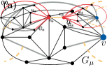
Figure 2: (a) A triconnected skeleton $G_{\mu}$ with a highlighted vertex $v$ incident to two gray virtual edges. (b) The result of applying IsolateVertex to isolate $v$ out of the skeleton. The red occupied edges in the old skeleton $G_{\alpha}$ form a star with center $v_{\alpha}$, while the red occupied edges in $G_{\beta}$ connect all neighbors of $v$ to form a star with center $v_{\beta}\neq v$. The centers $v_{\alpha}$ and $v_{\beta}$ are virtual and matched with each other. Neighbor $u$ of $v$ was split into vertices $u_{\alpha}$ and $u_{\beta}$.

The operations IsolateVertex and Integrate now allow us to isolate vertices out of triconnected components and integrate them back in, respectively. For IsolateVertex, let $v$ be a non-virtual vertex of skeleton $G_{\mu}$, such that $v$ has no incident occupied edges. Applying ${\texttt{Iso\-late\-Ver\-tex}}(\mathcal{S},v)$ on an extended skeleton decomposition $\mathcal{S}$ yields an extended skeleton decomposition $\mathcal{S}^{\prime}=(\mathcal{G}^{\prime},\allowbreak\operatorname{origV}^{\prime},\allowbreak\operatorname{origE}^{\prime},\allowbreak\operatorname{twinE}^{\prime},\allowbreak\operatorname{twinV}^{\prime})$ as follows. Each neighbor $u$ of $v$ is split into two non-adjacent vertices $u_{\alpha}$ and $u_{\beta}$, where $u_{\beta}$ is incident to all edges connecting $u$ with $v$, while $u_{\alpha}$ keeps all other edges of $u$. We set $\operatorname{origV}^{\prime}(u_{\alpha})=\operatorname{origV}^{\prime}(u_{\beta})=\operatorname{origV}(u)$. This creates an independent, star-shaped component with center $v$, which we move to skeleton $G_{\beta}$, while we rename skeleton $G_{\mu}$ to $G_{\alpha}$. We connect all $u_{\alpha}$ to a single new virtual vertex $v_{\alpha}\in V_{\alpha}^{\textrm{virt}}$ using occupied edges, and all $u_{\beta}$ to a single new virtual vertex $v_{\beta}\in V_{\beta}^{\textrm{virt}}$ using occupied edges; see Figure 2. Finally, we set $\operatorname{twinV}^{\prime}(v_{\alpha})=v_{\beta}$, $\operatorname{twinV}^{\prime}(v_{\beta})=v_{\alpha}$, and add $G_{\beta}$ to $\mathcal{G}^{\prime}$. All other mappings and skeletons remain unchanged.

For Integrate, consider two virtual vertices $v_{\alpha},v_{\beta}$ with $\operatorname{twinV}(v_{\alpha})=v_{\beta}$ and the bijection $\gamma_{v_{\alpha}v_{\beta}}$ between the neighbors of $v_{\alpha}$ and $v_{\beta}$. An application of ${\texttt{In\-te\-grate}}(\mathcal{S},(v_{\alpha},v_{\beta}))$ yields an extended skeleton decomposition $\mathcal{S}^{\prime}=(\mathcal{G}^{\prime},\allowbreak\operatorname{origV}^{\prime},\allowbreak\operatorname{origE}^{\prime},\allowbreak\operatorname{twinE}^{\prime},\allowbreak\operatorname{twinV}^{\prime})$ as follows. We merge both skeletons into a skeleton $G_{\mu}$ (also replacing both in $\mathcal{G}^{\prime}$) by identifying the neighbors of $v_{\alpha}$ and $v_{\beta}$ according to $\gamma_{v_{\alpha}v_{\beta}}$. Furthermore, we remove $v_{\alpha}$ and $v_{\beta}$ together with their incident occupied edges. All other mappings and skeletons remain unchanged.

Lemma 4.1.

Applying IsolateVertex or Integrate on an extended skeleton decomposition $\mathcal{S}=(\mathcal{G},\allowbreak\operatorname{origV},\allowbreak\operatorname{origE},\allowbreak\operatorname{twinE},\allowbreak\operatorname{twinV})$ yields an extended skeleton decomposition $\mathcal{S}^{\prime}=(\mathcal{G}^{\prime},\allowbreak\operatorname{origV}^{\prime},\allowbreak\operatorname{origE}^{\prime},\allowbreak\operatorname{twinE}^{\prime},\allowbreak\operatorname{twinV}^{\prime})$ with $G_{\mathcal{S^{\prime}}}=G_{\mathcal{S}}$.

Proof 4.2.

We first check that all conditions still hold in the extended skeleton decomposition $\mathcal{S}^{\prime}$ returned by IsolateVertex. Condition LABEL:cond:bicon remains satisfied, as the structure of $G_{\alpha}$ remains unchanged compared to $G_{\mu}$ and the skeleton $G_{\beta}$ is a bond. As we are again splitting a node of $T_{\mathcal{S}}$, condition LABEL:cond:tree also remains satisfied. Due to the neighbors of $v_{\beta}$ and $v_{\alpha}$ mapping to the same vertices of $G_{\mathcal{S^{\prime}}}$, conditions LABEL:cond:orig-inj, LABEL:cond:orig-real, and LABEL:cond:orig-virt remain satisfied. Conditions LABEL:cond:stars and LABEL:cond:orig-stars are satisfied by construction.

Lastly, condition LABEL:cond:subgraph could only be violated if the subgraph of $T_{\mathcal{S^{\prime}}}$ formed by the allocation skeletons of some vertex $z\in G_{\mathcal{S^{\prime}}}$ was no longer connected. This could only happen if only one of $G_{\alpha}$ and $G_{\beta}$ were an allocation skeleton of $z$, while the other has a further neighbor $G_{\nu}$ that is also an allocation skeleton of $z$. Note that in any case, $\nu$ is adjacent to $\mu$ in $T_{\mathcal{S}}$ and $\mu$ must be an allocation skeleton of $z$, thus it is $z\in\operatorname{origV}(G_{\nu})\cap\operatorname{origV}(G_{\mu})$. Depending on the adjacency of $\nu$, it is either $\operatorname{origV}(G_{\nu})\cap\operatorname{origV}(G_{\mu})=\operatorname{origV}^{\prime}(G_{\nu})\cap\operatorname{origV}(G_{\alpha})$ or $\operatorname{origV}(G_{\nu})\cap\operatorname{origV}(G_{\mu})=\operatorname{origV}^{\prime}(G_{\nu})\cap\operatorname{origV}(G_{\beta})$, as $\nu$ is not modified by the operation and both $\mathcal{S}$ and $\mathcal{S}^{\prime}$ satisfy LABEL:cond:orig-virt and LABEL:cond:orig-stars. This immediately contradicts the skeleton of $\{\alpha,\beta\}$, that is adjacent to $\nu$, not being an allocation skeleton of $z$.

Finally, the mapping $\operatorname{origE}$ remains unchanged and the only change to $\operatorname{origV}$ is to include some duplicated vertices mapping to already existing vertices. Due to condition LABEL:cond:orig-real holding for both the input and the output instance, this cannot affect the represented graph $G_{\mathcal{S^{\prime}}}$.

Now consider the extended skeleton decomposition $\mathcal{S}^{\prime}$ returned by Integrate. The merged skeleton is biconnected, as we are effectively replacing a single vertex by a connected subgraph, satisfying LABEL:cond:bicon. The operation effectively contracts and removes an edge in $T_{\mathcal{S}}$, which does not affect $T_{\mathcal{S^{\prime}}}$ being a tree, satisfying condition LABEL:cond:tree. Note that condition LABEL:cond:tree holding for the input instance also ensures that $v_{\alpha}$ and $v_{\beta}$ belong to two distinct skeletons. As the input instance satisfies condition LABEL:cond:orig-virt, the vertices in each of the two adjacent skeletons where $\operatorname{origV}$ maps to the same vertex of $G_{\mathcal{S}}$ are exactly the neighbors of the matched $v_{\alpha}$ and $v_{\beta}$. Thus, $\operatorname{origV}|_{V_{\alpha}}$ is still injective, satisfying condition LABEL:cond:orig-inj. As we modify no real or virtual edges, the mappings $\operatorname{origV}^{\prime},\operatorname{origE}^{\prime}$ and $\operatorname{twinE}^{\prime}$ obviously still satisfy conditions LABEL:cond:orig-real and LABEL:cond:orig-virt. Finally, contracting a tree edge cannot lead to any of the subgraphs of LABEL:cond:subgraph becoming disconnected, thus the condition also remains satisfied. Conditions LABEL:cond:stars and LABEL:cond:orig-stars also remain unaffected, as we simply remove an entry from $\operatorname{twinV}$.

Again, no changes were made to $\operatorname{origE}$, while condition LABEL:cond:orig-stars makes sure that $\operatorname{origV}$ mapped each pair of merged vertices to the same vertex of $G_{\mathcal{S}}$. Thus, the represented graph $G_{\mathcal{S^{\prime}}}$ remains unchanged.

Furthermore, as Integrate is the converse of IsolateVertex and has no preconditions, any changes made by IsolateVertex can be undone at any time to obtain a (non-extended) skeleton decomposition, and thus possibly the SPQR-tree of the represented graph.

Remark 4.3.

Exhaustively applying Integrate to an extended skeleton decomposition $\mathcal{S}=(\mathcal{G},\allowbreak\operatorname{origV},\allowbreak\operatorname{origE},\allowbreak\operatorname{twinE},\allowbreak\operatorname{twinV})$ yields a extended skeleton decomposition $\mathcal{S}^{\prime}=(\mathcal{G}^{\prime},\allowbreak\operatorname{origV}^{\prime},\allowbreak\operatorname{origE}^{\prime},\allowbreak\operatorname{twinE}^{\prime},\allowbreak\operatorname{twinV}^{\prime})$ where $\operatorname{twinV}^{\prime}=\emptyset$. Thus, $\mathcal{S}^{\prime}$ is equivalent to a (non-extended) skeleton decomposition $\mathcal{S}^{\prime}=(\mathcal{G}^{\prime},\allowbreak\operatorname{origV}^{\prime},\allowbreak\operatorname{origE}^{\prime},\allowbreak\operatorname{twinE}^{\prime})$.

5 Node Expansion in Extended Skeleton Decompositions

Figure 3: Expanding a skeleton vertex $v$ into a graph $G_{\nu}$ in the SPQR-tree of Figure 4. (a) The single allocation skeleton $G_{\mu}$ of $u$ with the single allocation vertex $v$ of $u$ from Figure 4. The neighbors of $v$ are marked in orange. (b) The inserted graph $G_{\nu}$ with orange marked vertices. Note that the graph is biconnected when all marked vertices are collapsed into a single vertex. (c) The result of applying ${\texttt{In\-sert\-Graph}}(\mathcal{S},u,G_{\nu},\phi)$ followed by an application of Integrate on the generated virtual vertices $v$ and $v^{\prime}$.

We now introduce our first dynamic operation that allows us to actually change the represented graph by expanding a single vertex $u$ into an arbitrary connected graph $G_{\nu}$. This is done by identifying $|N(u)|$ marked vertices in $G_{\nu}$ with the neighbors of $u$ via a bijection $\phi$ and then removing $u$ and its incident edges. We use the “occupied stars” from the previous section to model the identification of these vertices, allowing us to defer the actual insertion to an application of Integrate. We need to ensure that the inserted graph makes the same “guarantees” to the surrounding graph in terms of connectivity as the vertex it replaces, that is all neighbors of $u$ (i.e. all marked vertices in $G_{\nu}$) need to be pairwise connected via paths in $G_{\nu}$ not using any other neighbor of $u$ (i.e. any other marked vertex). Without this requirement, a single vertex could e.g. also be split into two non-adjacent halves, which could easily break a triconnected component apart. Thus, we require $G_{\nu}$ to be biconnected when all marked vertices are collapsed into a single vertex. Note that this also ensures that the old graph can be restored by contracting the vertices of the inserted graph. For the sake of simplicity, we require vertex $u$ from the represented graph to have a single allocation vertex $v\in G_{\mu}$ with $\operatorname{origV}^{-1}(u)=\{v\}$ so that we only need to change a single allocation skeleton $G_{\mu}$ in the skeleton decomposition. As we will make clear later on, this condition can be satisfied easily.

Formally, let $u\in G_{\mathcal{S}}$ be a vertex that only has a single allocation vertex $v\in G_{\mu}$ (and thus only a single allocation skeleton $G_{\mu}$). Let $G_{\nu}$ be an arbitrary, new graph containing $|N(u)|$ marked vertices, together with a bijection $\phi$ between the marked vertices in $G_{\nu}$ and the neighbors of $v$ in $G_{\mu}$. We require $G_{\nu}$ to be biconnected when all marked vertices are collapsed into a single node. Operation ${\texttt{In\-sert\-Graph}}(\mathcal{S},u,G_{\nu},\phi)$ yields an extended skeleton decomposition $\mathcal{S}^{\prime}=(\mathcal{G}^{\prime},\allowbreak\operatorname{origV}^{\prime},\allowbreak\operatorname{origE}^{\prime},\allowbreak\operatorname{twinE}^{\prime},\allowbreak\operatorname{twinV}^{\prime})$ as follows, see also Figure 3. We interpret $G_{\nu}$ as skeleton and add it to $\mathcal{G}^{\prime}$. For each marked vertex $x$ in $G_{\nu}$, we set $\operatorname{origV}^{\prime}(x)=\operatorname{origV}(\phi(x))$. For all other vertices and edges in $G_{\nu}$, we set $\operatorname{origV}^{\prime}$ and $\operatorname{origE}^{\prime}$ to point to new vertices and edges forming a copy of $G_{\nu}$ in $\mathcal{G}_{\mathcal{S^{\prime}}}$. We connect every marked vertex in $G_{\nu}$ to a new virtual vertex $v^{\prime}\in G_{\nu}$ using occupied edges. We also convert $v$ to a virtual vertex, converting its incident edges to occupied edges while removing parallel edges. Finally, we set $\operatorname{twinV}^{\prime}(v)=v^{\prime}$ and $\operatorname{twinV}^{\prime}(v^{\prime})=v$.

Lemma 5.1.

Applying ${\texttt{In\-sert\-Graph}}(\mathcal{S},u,G_{\nu},\phi)$ on an extended skeleton decomposition $\mathcal{S}=(\mathcal{G},\allowbreak\operatorname{origV},\allowbreak\operatorname{origE},\allowbreak\operatorname{twinE},\allowbreak\operatorname{twinV})$ yields an extended skeleton decomposition $\mathcal{S}^{\prime}=(\mathcal{G}^{\prime},\allowbreak\operatorname{origV}^{\prime},\allowbreak\operatorname{origE}^{\prime},\allowbreak\operatorname{twinE}^{\prime},\allowbreak\operatorname{twinV}^{\prime})$ with $G_{\mathcal{S^{\prime}}}$ isomorphic to $G_{\mathcal{S}}[u\rightarrow_{\phi}G_{\nu}]$.

Proof 5.2.

Condition LABEL:cond:bicon remains satisfied, as the structure of $G_{\mu}$ remains unchanged and the resulting $G_{\nu}$ is biconnected by precondition. Regarding $T_{\mathcal{S}}$, we are attaching a degree-1 node $\nu$ to an existing node $\mu$, thus condition LABEL:cond:tree also remains satisfied. As all vertices of $G_{\nu}$ except for the vertices in $N(v^{\prime})$ got their new, unique copy assigned by $\operatorname{origV}^{\prime}$ and $\operatorname{origV}^{\prime}(N(v^{\prime}))=\operatorname{origV}(N(v))$, condition LABEL:cond:orig-inj is also satisfied for the new $G_{\nu}$. As we updated $\operatorname{origE}$ alongside $\operatorname{origV}$ and $G_{\nu}$ contains no virtual edges, conditions LABEL:cond:orig-real and LABEL:cond:orig-virt remain satisfied. As $\nu$ is a leaf of $T_{\mathcal{S}}$ with $\mu$ being its only neighbor, $\operatorname{origV}^{\prime}(N(v^{\prime}))\subset\operatorname{origV}(V_{\mu})$, and $G_{\nu}$ is the only allocation skeleton for all vertices in $G_{\nu}\setminus N(v^{\prime})$, condition LABEL:cond:subgraph remains satisfied. Conditions LABEL:cond:stars and LABEL:cond:orig-stars are satisfied by construction. Finally, the mappings $\operatorname{origE}^{\prime}$ and $\operatorname{origV}^{\prime}$ are by construction updated to correctly reproduce the structure of $G_{\nu}$ in $G_{\mathcal{S^{\prime}}}$.

On its own, this operation is not of much use though, as graph vertices only rarely have a single allocation skeleton. Furthermore, our goal is to dynamically maintain SPQR-trees, while this operation on its own will in most cases not yield an SPQR-tree. To fix this, we introduce the full procedure ${\texttt{In\-sert}\-\texttt{Graph}_{\texttt{SPQR}}}(\mathcal{S},u,G_{\nu},\phi)$ that can be applied to any graph vertex $u$ and that, given an SPQR-tree $\mathcal{S}$, yields the SPQR-tree of $G_{\mathcal{S}}[u\rightarrow_{\phi}G_{\nu}]$. It consists of three preparations steps, the insertion of $G_{\nu}$, and two further clean-up steps:

1. We apply SplitSeparationPair to each polygon allocation skeleton of $u$ with more than three vertices, using the neighbors of the allocation vertex of $u$ as separation pair.

2. For each rigid allocation skeleton of $u$, we move the contained allocation vertex $v$ of $u$ to its own skeleton by applying ${\texttt{Iso\-late\-Ver\-tex}}(\mathcal{S},v)$.

3. We exhaustively apply JoinSeparationPair to any pair of allocation skeletons of $u$ that are adjacent in $T_{\mathcal{S}}$. Due to condition LABEL:cond:subgraph, this yields a single component $G_{\mu}$ that is the sole allocation skeleton of $u$ with the single allocation vertex $v$ of $u$. Furthermore, the size of $G_{\mu}$ is linear in $\deg(u)$.

4. We apply InsertGraph to insert $G_{\nu}$ as skeleton, followed by an application of Integrate to the virtual vertices $\{v,v^{\prime}\}$ introduced by the insertion, thus integrating $G_{\nu}$ into $G_{\mu}$.

5. We apply SplitSeparationPair to all separation pairs in $G_{\mu}$ that do not involve a virtual vertex. These pairs can be found in linear time, e.g. by temporarily duplicating all virtual vertices and their incident edges and then computing the SPQR-tree.

6. Finally, we exhaustively apply Integrate and also apply JoinSeparationPair to any two adjacent polygons and to any two adjacent bonds to obtain the SPQR-tree of the updated graph.

Figure 4: The preprocessing steps of Insert$\texttt{Graph}_{\texttt{SPQR}}$ being applied to the SPQR-tree of Figure 1. (a) The state after Item 2, after all allocation skeletons of $u$ have been split. (b) The state after Item 3, after all allocation skeletons of $u$ have been merged into a single one.

The basic idea behind the correctness of this procedure is that splitting the newly inserted component according to its SPQR-tree in Item 5 yields biconnected components that are each either a polygon, a bond, or “almost” triconnected. The latter (and only those) might still contain virtual vertices and all their remaining separation pairs, which were not split in Item 5, contain one of these virtual vertices. This, together with the fact that there still may be pairs of adjacent skeletons where both are polygons or both are bonds, prevents the instance from being an SPQR-tree. Both issues are resolved in Item 6: The adjacent skeletons are obviously fixed by the JoinSeparationPair applications. To show that the virtual vertices are removed by the Integrate applications, making the remaining components triconnected, we need the following lemma.

Lemma 5.3.

Let $G_{\alpha}$ be a triconnected skeleton containing a virtual vertex $v_{\alpha}$ matched with a virtual vertex $v_{\beta}$ of a biconnected skeleton $G_{\beta}$. Furthermore, let $P\subseteq\binom{V(G_{\beta})}{2}$ be the set of all separation pairs in $G_{\beta}$. An application of ${\texttt{In\-te\-grate}}(\mathcal{S},(v_{\alpha},v_{\beta}))$ yields a biconnected skeleton $G_{\mu}$ with separation pairs $P^{\prime}=\{\{u,v\}\in P\mid v_{\beta}\notin\{u,v\}\}$.

Proof 5.4.

We partition the vertices of $G_{\mu}$ into the sets $A,B$, and $N$ depending on whether the vertex stems from $G_{\alpha}$, $G_{\beta}$, or both, respectively. The set $N$ thus contains the neighbors of $v_{\alpha}$, which were identified with the neighbors of $v_{\beta}$. We will now show by contradiction that $G_{\mu}$ contains no separation pairs except for those in $P^{\prime}$. Thus, consider a separation pair $u,v\in G_{\mu}$ not in $P^{\prime}$. First, consider the case where $u,v\in A\cup N$. Observe that removing $u,v$ in this case leaves $B$ connected. Thus, we can contract all vertices of $B$ into a single vertex, reobtain $G_{\alpha}$ and see that $u,v$ is a separation pair in $G_{\alpha}$. This contradicts the precondition that $G_{\alpha}$ is triconnected. Now consider the case where $u,v\in B\cup N$. Analogously to above, we find that $u,v$ is a separation pair in $G_{\beta}$ that does not contain $v_{\beta}$, a contradiction to $\{u,v\}\notin P^{\prime}$. Finally, consider the remaining case where, without loss of generality, $u\in A,v\in B$. Since $\{u,v\}$ is a separation pair, $u$ has two neighbors $x,y$ that lie in different connected components of $G_{\mu}-\{u,v\}$ and therefore also in different components of $(G_{\mu}-\{u,v\})-B$ which is isomorphic to $G_{\alpha}-\{u,v_{\alpha}\}$. This again contradicts the precondition that $G_{\alpha}$ is triconnected.

Theorem 5.5.

Applying ${\texttt{In\-sert}\-\texttt{Graph}_{\texttt{SPQR}}}(\mathcal{S},u,G_{\nu},\phi)$ to an SPQR-tree $\mathcal{S}$ yields an SPQR-tree $\mathcal{S}^{\prime}$ in $O(|G_{\nu}|)$ time with $G_{\mathcal{S^{\prime}}}$ isomorphic to $G_{\mathcal{S}}[u\rightarrow_{\phi}G_{\nu}]$.

Proof 5.6.

As all operations that are applied leave the extended skeleton decomposition valid, the final extended skeleton decomposition $\mathcal{S}^{\prime}$ is also valid. Observe that the purpose of the preprocessing Items 1, 3 and 2 is solely to ensure that the preconditions of InsertGraph are satisfied and the affected component is not too large. Note that all rigids split in Item 2 remain structurally unmodified in the sense that edges only changed their type, but the graph and especially its triconnectedness remains unchanged. Item 4 performs the actual insertion and yields the desired represented graph according to Lemma 5.1. It thus remains to show that the clean-up steps turn the obtained extended skeleton decomposition into an SPQR-tree. Applying Integrate exhaustively in Item 6 ensures that the extended skeleton decomposition is equivalent to a non-extended one (Remark 4.3). Recall that a non-extended skeleton decomposition is an SPQR-tree if all skeletons are either polygons, bonds or triconnected and two adjacent skeletons are never both polygons or both bonds (Definition 3.5). Item 6 ensures that the second half holds, as joining two polygons (or two bonds) with JoinSeparationPair yields a bigger polygon (or bond, respectively). Before Item 6, all skeletons that are not an allocation skeleton of $u$ are still unmodified and thus already have a suitable structure, i.e., they are either polygons, bonds or triconnected. Furthermore, the allocation skeletons of $u$ not containing virtual vertices also have a suitable structure, as their splits were made according to the SPQR-tree in Item 5. It remains to show that the remaining skeletons, that is those resulting from the Integrate applications in Item 6, are triconnected. Note that in these skeletons, Item 5 ensures that every separation pair consists of at least one virtual vertex, as otherwise the computed SPQR-tree would have split the skeleton further. Further note that, for each of these virtual vertices, the matched partner vertex is part of a structurally unmodified triconnected skeleton that was split in Item 2. Lemma 5.3 shows that applying Integrate does not introduce new separation pairs while removing two virtual vertices if one of the two sides is triconnected. We can thus exhaustively apply Integrate and thereby remove all virtual vertices and thus also all separation pairs, obtaining triconnected components. This shows that the criteria for being an SPQR-tree are satisfied and, as InsertGraph expanded $u$ to $G_{\nu}$ in the represented graph, we now have the unique SPQR-tree of $G_{\mathcal{S}}[u\rightarrow_{\phi}G_{\nu}]$.

Note that all operations we used can be performed in time linear in the degree of the vertices they are applied on. For the bipartition of bridges input to SplitSeparationPair, it is sufficient to describe each bridge via its edges incident to the separation pair instead of explicitly enumerating all in vertices in the bridge. Thus, the applications of SplitSeparationPair and IsolateVertex in Items 1 and 2 touch every edge incident to $u$ at most once and thus take $O(\deg(u))$ time. Furthermore, they yield skeletons that have a size linear in the degree of their respective allocation vertex of $u$. As the subtree of $u$’s allocation skeletons has size at most $\deg(u)$, the JoinSeparationPair applications of Item 3 also take at most $O(\deg(u))$ time. It also follows that the resulting single allocation skeleton of $u$ has size $O(\deg(u))$. The applications of InsertGraph and Integrate in Item 4 can be done in time linear in the number of identified neighbors, which is $O(\deg(u))$. Generating the SPQR-tree of the inserted graph in Item 5 (where all virtual vertices where replaced by wheels) can be done in time linear in the size of the inserted graph [30, 33], that is $O(|G_{\nu}|)$. Applying SplitSeparationPair according to all separation pairs identified by this SPQR-tree can also be done in $O(|G_{\nu}|)$ time in total. Note that there are at most $\deg(u)$ edges between the skeletons that existed before Item 4 and those that were created or modified in Items 4 and 5, and these are the only edges that might now connect two polygons or two bonds. As these tree edges have one endpoint in the single allocation skeleton of $u$, the applications of Integrate and JoinSeparationPair in Item 6 run in $O(\deg(u))$ time in total. Furthermore, they remove all pairs of adjacent polygons and all pairs of adjacent bonds. This shows that all steps take $O(\deg(u))$ time, except for Item 5, which takes $O(|G_{\nu}|)$ time. As the inserted graph contains at least one vertex for each neighbor of $u$, the total runtime is in $O(|G_{\nu}|)$.

Corollary 5.7.

Let $\mathcal{S}_{1},\mathcal{S}_{2}$ be two SPQR-trees together with vertices $u_{1}\in G_{\mathcal{S}_{1}},$ $u_{2}\in G_{\mathcal{S}_{2}}$, and let $\phi$ be a bijection between the edges incident to $u_{1}$ and the edges incident to $u_{2}$. Operation ${\texttt{Merge}_{\texttt{SPQR}}}(\mathcal{S}_{1},\mathcal{S}_{2},u_{1},u_{2},\phi)$ yields the SPQR-tree of the graph $G_{\mathcal{S}_{1}}[u_{1}\rightarrow_{\phi}G_{\mathcal{S}_{2}}-u_{2}]$, i.e. the union of both graphs where the edges incident to $u_{1},u_{2}$ were identified according to $\phi$ and $u_{1},u_{2}$ removed, in time $O(\deg(u_{1}))=O(\deg(u_{2}))$.

Proof 5.8.

Operation $\texttt{Merge}_{\texttt{SPQR}}$ works similar to the more general Insert$\texttt{Graph}_{\texttt{SPQR}}$, although the running time is better because we already know the SPQR-tree for the graph being inserted. We apply the preprocessing Items 1, 2 and 3 to ensure that both $u_{1}$ and $u_{2}$ have sole allocation vertices $v_{1}$ and $v_{2}$, respectively. To properly handle parallel edges, we subdivide all edges incident to $u_{1},u_{2}$ (and thus also the corresponding real edges incident to $v_{1},v_{2}$) and then identify the subdivision vertices of each pair of edges matched by $\phi$. By deleting vertices $v_{1}$ and $v_{2}$ and suppressing the subdivision vertices (that is, removing them and identifying each pair of incident edges) we obtain a skeleton $G_{\mu}$ that has size $O(\deg(u_{1}))=O(\deg(u_{2}))$. Finally, we apply the clean-up Items 6 and 5 to $G_{\mu}$ to obtain the final SPQR-tree. Again, as the partner vertex of every virtual vertex in the allocation skeletons of $u$ is part of a triconnected skeleton, applying Integrate exhaustively in Item 6 yields triconnected skeletons. As previously discussed, the preprocessing and clean-up steps run in time linear in degree of the affected vertices, thus the overall runtime is $O(\deg(u_{1}))=O(\deg(u_{2}))$ in this case.

5.1 Maintaining Planarity and Vertex Rotations

Note that expanding a vertex of a planar graph using another planar graph using Insert$\texttt{Graph}_{\texttt{SPQR}}$ (or merging two SPQR-trees of planar graphs using Corollary 5.7) might actually yield a non-planar graph. This is, e.g., because the rigids of both graphs might require incompatible orders for the neighbors of the replaced vertex. The aim of this section is to efficiently detect this case, that is a planar graph turning non-planar. To check a general graph for planarity, it suffices to check the rigids in its SPQR-tree for planarity and each rigid allows exactly two planar embeddings, where one is the reverse of the other [19]. Thus, if a graph becomes non-planar through an application of Insert$\texttt{Graph}_{\texttt{SPQR}}$, this will be noticeable from the triconnected allocation skeletons of the replaced vertex. To be able to immediately report if the instance became non-planar, we need to maintain a rotation, that is a cyclic order of all incident edges, for each vertex in any triconnected skeleton. Note that we do not track the direction of the orders, that is we only store the order up to reversal. As discussed later, the exact orders can also be maintained with a slight overhead.

Theorem 5.9.

SPQR-trees support the following operations:

• ${\texttt{In\-sert}\-\texttt{Graph}_{\texttt{SPQR}}}(\mathcal{S},u,G_{\nu},\phi)$: expansion of a single vertex $u$ in time $O(|G_{\nu}|)$,

• ${\texttt{Merge}_{\texttt{SPQR}}}(\mathcal{S}_{1},\mathcal{S}_{2},u_{1},u_{2},\phi)$: merging of two SPQR-trees in time $O(\deg(u_{1}))$,

• IsPlanar: queries whether the represented graph is planar in time $O(1)$, and

• $\texttt{Rotation}(u)$: queries for one of the two possible rotations of vertices $u$ in planar triconnected skeletons in time $O(1)$.

Proof 5.10.

Note that the boolean flag IsPlanar together with the Rotation information can be computed in linear time when creating a new SPQR-tree and that expanding a vertex or merging two SPQR-trees cannot turn a non-planar graph planar. We make the following changes to the operations Insert$\texttt{Graph}_{\texttt{SPQR}}$ and $\texttt{Merge}_{\texttt{SPQR}}$ described in Theorem 5.5 and Corollary 5.7 to maintain the new information. After a triconnected component is split in Item 2 we now introduce further structure to ensure that the embedding is maintained on both sides. The occupied edges generated around the split-off vertex $v$ (and those around its copy $v^{\prime}$) are subdivided and connected cyclically according to Rotation$(v)$. Instead of “stars”, we thus now generate occupied “wheels” that encode the edge ordering in the embedding of the triconnected component. When generating the SPQR-tree of the modified subgraph in Item 5, now containing occupied wheels instead of only stars, we also generate a planar embedding for all its triconnected skeletons. If no planar embedding can be found for at least one skeleton, we report that the resulting instance is non-planar by setting IsPlanar to false. Otherwise, after performing all splits indicated by the SPQR-tree, we assign Rotation by generating embeddings for all new rigids. Note that for all skeletons with virtual vertices, the generated embedding will be compatible with the one of the neighboring triconnected component, that is, the rotation of each virtual vertex will line up with that of its matched partner vertex, thanks to the inserted wheel. Finally, before applying Integrate in Item 6, we contract each occupied wheel into a single vertex to re-obtain occupied stars. The creation and contraction of wheels adds an overhead that is at most linear in the degree of the expanded vertex and the generation of embeddings for the rigids can be done in time linear in the size of the rigid. Thus, this does not affect the asymptotic runtime of both operations.

Corollary 5.11.

The data structure from Theorem 5.9 can be adapted to also provide the exact rotations with matching direction for every vertex in a rigid. Furthermore, it can support queries whether two vertices $v_{1},v_{2}$ are connected by at least 3 different vertex-disjoint paths via $\texttt{3Paths}(v_{1},v_{2})$ in $O((\deg(v_{1})+\deg(v_{2}))\cdot\alpha(n))$ time. These adaptions change the runtime of ${\texttt{In\-sert}\-\texttt{Graph}_{\texttt{SPQR}}}$ to $O(\deg(u)\cdot\alpha(n)+|G_{\nu}|)$, that of ${\texttt{Merge}_{\texttt{SPQR}}}$ to $O(\deg(u_{1})\cdot\alpha(n))$, and that of $\texttt{Rotation}(u)$ to $O(\alpha(n))$.

Proof 5.12.

The exact rotation information for Rotation can be maintained by using union-find to keep track of the rigid a vertex belongs to and synchronizing the reversal of all vertices within one rigid when two rigids are merged by Integrate as follows. We create a union-find set for every vertex in a triconnected component and apply Union to all vertices in the same rigid. Next to the pointer indicating the representative in the union-find structure, we store a boolean flag indicating whether the rotation information for the current vertex is reversed with regard to rotation of its direct representative. To find whether a Rotation needs to be flipped, we accumulate all flags along the path to the actual representative of a vertex by using an exclusive-or. As $\texttt{Rotation}(u)$ thus relies on the Find operation, its amortized runtime is $O(\alpha(n))$. When merging two rigids with Integrate, we also perform a Union on their respective representatives (which we need to Find first), making ${\texttt{In\-te\-grate}}(\mathcal{S},(v_{\alpha},v_{\beta}))$ run in $O(\deg(v_{\alpha})+\alpha(n))$. We also compare the Rotation of the replaced vertices and flip the flag stored with the vertex that does not end up as the representative if they do not match. In total, this makes ${\texttt{In\-sert}\-\texttt{Graph}_{\texttt{SPQR}}}$ run in $O(\deg(u)\cdot\alpha(n)+|G_{\nu}|)$ time as there can be up to $\deg(u)$ split rigids. Furthermore, ${\texttt{Merge}_{\texttt{SPQR}}}$ now runs in $O(\deg(u_{1})\cdot\alpha(n))$ time.

Maintaining the information in which rigid a skeleton vertex is contained in can then also be used to answer queries whether two arbitrary vertices are connected by three disjoint paths. This is exactly the case if they are part of the same rigid, appear as poles of the same bond or are connected by a virtual edge in a polygon. This can be checked by enumerating all allocation skeletons of both vertices, which can be done in time linear in their degree. As finding each of the skeletons may require a Find call, the total runtime for this is in $O((\deg(v_{1})+\deg(v_{2}))\cdot\alpha(n))$.

6 Application to Synchronized Planarity

In this section, we will give some background on the historical development of and further details on the problems Clustered Planarity and Synchronized Planarity together with summary of the algorithm of Bläsius et al. for solving both problems. Furthermore, we will show how our and also previous work on dynamic SPQR-trees can be used in the context of both problems.

6.1 Background and Discussion

Lengauer [34] first discussed Clustered Planarity under a different name in 1989, which is why it was later independently rediscovered by Feng et al. [23] in 1995. Both gave polynomial-time algorithms for the case where the subgraph induced by any cluster is connected. In contrast, the question whether the general problem with disconnected clusters allows an efficient solution remained open for 30 years. In that time, polynomial-time algorithms were found for many special-cases [2, 15, 25, 29] before Fulek and Tóth [26] found an $O((n+d)^{8})$ solution in 2019. Shortly thereafter, Bläsius et al. [8] gave a solution with runtime in $O((n+d)^{2})$ that also exposes the main concepts needed to solve Clustered Planarity. The solution works via a linear-time reduction to the problem Synchronized Planarity, for which Bläsius et al. gave a quadratic algorithm. We improve the runtime of the latter algorithm. As Synchronized Planarity can be used as a modeling tool for several other constrained planarity problems next to Clustered Planarity [8], this also improves the time needed for solving any constrained planarity problem that can be solved via a linear-time reduction to Synchronized Planarity; see Table 1.

In Clustered Planarity, the embedding has to respect a laminar family of clusters [9, 34], that is every vertex is part of some (hierarchically nested) cluster and an edge may only cross a cluster boundary if it connects a vertex from the inside with one from the outside. In Synchronized Planarity, we are given a matching on some of the vertices in the graph and seek an embedding such that the rotations matched vertices line up under a given bijection [8]. The synchronization constraints imposed by matching two vertices are also called pipe. The reduction from the former problem to the latter employs the CD-tree representation of Clustered Planarity [9], where each cluster is represented as individual skeleton in which adjacent clusters were collapsed into single “virtual vertices”. The order of the edges “leaving” one cluster via a virtual vertex now needs to line up with the order in which they “enter” an adjacent cluster via its corresponding virtual vertex (see also [8, Figure 6]).

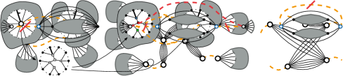
Figure 5: Schematic representation of the three operations used by Bläsius et al. [8] for solving Synchronized Planarity. Matched vertices are shown as bigger disks, the matching is indicated by the orange dotted lines. Top: Two cut-vertices matched with each other (left), the result of encapsulating their incident blocks (middle) and the bipartite graph resulting from joining both cut-vertices (right). Middle: A matched non-cut-vertex with a non-trivial embedding tree (left) that is propagated to replace both the vertex and its partner (right). Bottom: Three different cases of matched vertices with trivial embedding trees (blue) and how their pipes can be removed or replaced (red).

The algorithm for solving Synchronized Planarity works by removing an arbitrary pipe each step, using one of three operations depending on the graphs around the matched vertices, see Figure 5.

EncapsulateAndJoin

If both vertices of the pipe are cut-vertices, they are “encapsulated” by taking a copy of their respective components and then collapsing each incident block to a single vertex to obtain stars with matched centers that have multiple parallel edges connecting them to their ray vertices. The original cut-vertices are split up so that each incident block gets its own copy and these copies are synchronized with the respective vertex representing a collapsed block. Now the cut-vertices can be removed by “joining” both stars, that is identifying their incident edges according to the bijection that is given alongside the matching.

PropagatePQ

If one of the vertices is not a cut-vertex and has an embedding tree that not only consists of a single P-node, two copies of this embedding tree are inserted (“propagated”) in place of both matched vertices, respectively. The inner nodes of the embedding trees are synchronized by matching corresponding vertices.

SimplifyMatching

In the remaining case, one of the vertices is not a cut-vertex but has a trivial embedding tree, i.e., only appears in a single parallel skeleton and no rigid skeleton in the SPQR-tree. If the vertex (or, more precisely, the parallel that completely defines it rotation) can respect arbitrary rotations, we can simply remove the pipe. The only exception to this is when the other pole of the parallel is also matched, in which case we can “short-circuit” the matching across the parallel.

To summarize, every operation removes a pipe from the matching, while potentially introducing new pipes with vertices that have a smaller degree. Using a potential function, it can be shown that the progress made by the removal always dominates overhead of the newly-introduced pipes, and that the operations needed to remove all pipes is limited by the total degree of all matched vertices. Furthermore, the resulting instance without pipes can be solved in linear time. All of the three operations run in time linear in the degree of the un-matched vertices if the embedding trees they depend on are available. The contribution of this paper is to efficiently provide the embedding trees, which would require processing entire connected components at each step when done naïvely. Using the fully-dynamic SPQR-tree by Holm and Rotenberg [31, 32], this can be achieved with a poly-log cost of $O(\Delta\cdot\log^{3}n)$ leading to an overall runtime of $O(m\cdot\Delta\cdot\log^{3}n)$. Using the node expansion from this paper, we can improve the runtime from spending time linear in the size of the input instance ($O(m)$) for each of the linearly many operations, to only spending time linear in the maximum degree ($O(\Delta)$) on each operation. The reduction from Clustered Planarity creates an instance of size $O(n+d)$ in which the total degree of matched vertices is in $O(d)$, corresponding to the total number of times an edge crosses a cluster boundary. Note that, while this means that $O(d)$ operations are sufficient to reach a reduced instance, the number of crossings between edges and cluster boundaries can be quadratic in the number of vertices in a planar graph. We also note that while the improvement over using the Holm and Rotenberg approach is only poly-logarithmic, our datastructure has the additional benefit of being conceptually simpler and thus also more likely to improve performance in practice.

6.2 Using Node Expansion for Solving Synchronized Planarity

We show how extended skeleton decompositions and their dynamic operation Insert$\texttt{Graph}_{\texttt{SPQR}}$ can be used to improve the runtime of the algorithm for solving Synchronized Planarity by Bläsius et al. [8] from $O(m^{2})$ to $O(m\cdot\Delta)$, where $\Delta$ is the maximum pipe degree. As already explained in the previous section, the algorithm spends a major part of its runtime on computing so-called embedding trees, which describe all possible rotations of a single vertex in a planar graph and are used to communicate embedding restrictions between vertices with synchronized rotation. Once the embedding trees are available, the at most $O(m)$ executed operations run in time linear in the degree of the pipe/vertex they are applied on, that is in $O(\Delta)$ [8]. Thus, being able to generate these embedding trees efficiently by maintaining the SPQR-trees they are derived from is our main contribution towards the speedup of the Synchronized Planarity algorithm.

An embedding tree $\mathcal{T}_{v}$ for a vertex $v$ of a biconnected graph $G$ describes the possible cyclic orderings or rotations of the edges incident to $v$ in all planar embeddings of $G$ [12]. The leaves of $\mathcal{T}_{v}$ are the edges incident to $v$, while its inner nodes are partitioned into two categories: Q-nodes define an up-to-reversal fixed rotation of their incident tree edges, while P-nodes allow arbitrary rotation; see Figure 1. To generate the embedding tree we use the observation about the relationship of SPQR-trees and embedding trees described by Bläsius and Rutter [10, Section 2.5]: there is a bijection between the P- and Q-nodes in the embedding tree of $v$ and the bond and triconnected allocation skeletons of $v$ in the SPQR-tree of $G$, respectively.

Lemma 6.1.

Let $\mathcal{S}$ be an SPQR-tree with a planar represented graph $G_{\mathcal{S}}$. The embedding tree for a vertex $v\in G_{\mathcal{S}}$ can be found in time $O(\deg(v))$.

Proof 6.2.

We use the rotation information from Theorem 5.9 and furthermore maintain an (arbitrary) allocation vertex for each vertex in $G_{\mathcal{S}}$. To compute the embedding tree of a vertex $v$ starting at the allocation vertex $u$ of $v$, we will explore the SPQR-tree by using $\operatorname{twinE}$ on one of the edges incident to $u$ and then finding the next allocation vertex of $v$ as one endpoint of the obtained edge. If $u$ has degree 2, it is part of a polygon skeleton that does not induce a node in the embedding tree. We thus move on to its neighboring allocation skeletons and will also similarly skip over any other polygon skeleton we encounter. If $u$ has degree 3 or greater, we inspect two arbitrary incident edges: if they lead to the same vertex, $u$ is the pole of a bond, and we generate a P-node. Otherwise it is part of a triconnected component, and we generate a Q-node. We now iterate over the edges incident to $u$, in the case of a triconnected component using the order given by the rotation of $u$. For each real edge, we attach a corresponding leaf to the newly generated node. The graph edge corresponding to the leaf can be obtained from $\operatorname{origE}$. For each virtual edge, we recurse on the respective neighboring skeleton and attach the recursively generated node to the current node. As $u$ can only be part of $\deg(u)$ many skeletons, which form a subtree of $T_{\mathcal{S}}$, and the allocation vertices of $u$ in total only have $O(\deg(u))$ many virtual and real edges incident, this procedure yields the embedding tree of $u$ in time linear in its degree.

Our data structure can now be used to reduce the runtime of solving Synchronized Planarity by generating an SPQR-tree upfront, maintaining it throughout all applied operations, and deriving any needed embedding tree from the SPQR-tree.

Theorem 6.3.

Synchronized Planarity can be solved in time in $O(m\cdot\Delta)$, where $m$ is the number of edges and $\Delta$ is the maximum degree of a pipe.

Proof 6.4.

The algorithm works by splitting the pipes representing synchronization constraints until they are small enough to be trivial. It does so by exhaustively applying the three operations EncapsulateAndJoin, PropagatePQ and SimplifyMatching depending on the graph structure around the pairs of synchronized vertices. As mentioned by Bläsius et al., all operations run in time linear in the degree of the pipe they are applied on if the used embedding trees are known, and $O(m)$ operations are sufficient to solve a given instance [8]. Our modification is that we maintain an SPQR-tree for each biconnected component and then generate the needed embedding trees on-demand in linear time using Lemma 6.1. See Section 6.1 for more background on the Synchronized Planarity operations modified in the following.

Operation SimplifyMatching can be applied if the graph around a synchronized vertex $v$ allows arbitrary rotations of $v$, that is the embedding tree of $v$ is trivial. In this case, the pipe can be removed without modifying the graph structure. Thus, we can now easily check the preconditions of this operations without making any changes to the SPQR-tree.

PropagatePQ takes the non-trivial embedding tree of one synchronized vertex $v$ and inserts copies of the tree in place of $v$ and its partner, respectively. Synchronization constraints on the inner vertices of the inserted trees are used to ensure that they are embedded in the same way. We use Insert$\texttt{Graph}_{\texttt{SPQR}}$ to also insert the embedding tree into the respective SPQR trees, representing Q-nodes using wheels. When propagating into a cutvertex we also need to check whether two or more incident blocks merge. We form equivalence classes on the incident blocks, where two blocks are in the same class if 1) the two subtrees induced by their respective edges share at least two nodes 2) both induced subtrees share a C-node that has degree at least 2 in both subtrees. Blocks in the same equivalence class will end up in the same biconnected component as follows: We construct the subtree induced by all edges in the equivalence class and add a single further node for each block in the class, connecting all leaves to the node of the block the edges they represent lead to. We calculate the SPQR-tree for this biconnected graph and then merge the SPQR-trees of the individual blocks into it by applying Corollary 5.7. As Insert$\texttt{Graph}_{\texttt{SPQR}}$ (and similarly all $\texttt{Merge}_{\texttt{SPQR}}$ applications) runs in time linear in the size of the inserted PQ-tree, which is limited by the degree of the vertex it represents, this does not negatively impact the running time of the operation.

Operation EncapsulateAndJoin generates a new bipartite component representing how the edges of the blocks incident to two synchronized cutvertices are matched with each other. The size of this component is linear in the degree of the synchronized vertices. Thus, we can freshly compute the SPQR-tree for the generated component in linear time, which also does not negatively impact the running time.

Furthermore, as we now no longer need to iterate over whole connected components to generate the embedding trees, we are also no longer required to ensure those components do not grow to big. We can thus also directly contract pipes between two distinct biconnected components using Corollary 5.7 instead of having to insert PQ-trees using PropagatePQ. This may improve the practical runtime, as PropagatePQ might require further operations to clean up the generated pipes, while the direct contraction entirely removes a pipe without generating new ones.

Corollary 6.5.

Clustered Planarity can be solved in time in $O(n+d\cdot\Delta)$, where $d$ is the total number of crossings between cluster borders and edges and $\Delta$ is the maximum number of edge crossings on a single cluster border.

Proof 6.6.

Note that for a graph not containing parallel edges to be planar, the number of edges has to be linear in the number of vertices. We apply the reduction from Clustered Planarity to Synchronized Planarity as described by Bläsius et al. [8]. Ignoring the parallel edges generated by the CD-tree, we can generate an SPQR-tree for every component of the resulting instance in $O(n)$ time in total. The instance contains one pipe for every cluster boundary, where the degree of a pipe corresponds to the number of edges crossing the respective cluster boundary. Thus, the potential described by Bläsius et al. [8], which sums up the degrees of all pipes with a constant factor depending on the endpoints of each pipe, is in $O(d)$. Each operation applied when solving the Synchronized Planarity instance runs in time $O(\Delta)$ (the maximum degree of a pipe) and reduces the potential by at least 1. Thus, a reduced instance without pipes, which can be solved in linear time, can be reached in $O(d\cdot\Delta)$ time.

References

- [1] P. Angelini, T. Bläsius, and I. Rutter. Testing mutual duality of planar graphs. International Journal of Computational Geometry & Applications, 24(4):325–346, 2014. arXiv:1303.1640, doi:10.1142/S0218195914600103.
- [2] P. Angelini and G. Da Lozzo. Clustered planarity with pipes. Algorithmica, 81(6):2484–2526, 2019. doi:10.1007/s00453-018-00541-w.
- [3] P. Angelini, G. Di Battista, and M. Patrignani. Finding a minimum-depth embedding of a planar graph in time. Algorithmica, 60(4):890–937, 2009. doi:10.1007/s00453-009-9380-6.
- [4] P. Angelini, G. D. Lozzo, G. Di Battista, and F. Frati. Strip planarity testing for embedded planar graphs. Algorithmica, 77(4):1022–1059, 2016. doi:10.1007/s00453-016-0128-9.
- [5] T. C. Biedl, G. Kant, and M. Kaufmann. On triangulating planar graphs under the four-connectivity constraint. Algorithmica, 19(4):427–446, 1997. doi:10.1007/PL00009182.
- [6] D. Bienstock and C. L. Monma. Optimal enclosing regions in planar graphs. Networks, 19(1):79–94, 1989. doi:10.1002/net.3230190107.
- [7] D. Bienstock and C. L. Monma. On the complexity of embedding planar graphs to minimize certain distance measures. Algorithmica, 5(1):93–109, 1990. doi:10.1007/bf01840379.
- [8] T. Bläsius, S. D. Fink, and I. Rutter. Synchronized planarity with applications to constrained planarity problems. In Proceedings of the 29th Annual European Symposium on Algorithms (ESA’21), volume 204 of LIPIcs, pages 19:1–19:14, 2021. doi:10.4230/LIPIcs.ESA.2021.19.
- [9] T. Bläsius and I. Rutter. A new perspective on clustered planarity as a combinatorial embedding problem. Theoretical Computer Science, 609:306–315, 2016. arXiv:1506.05673, doi:10.1016/j.tcs.2015.10.011.
- [10] T. Bläsius and I. Rutter. Simultaneous PQ-ordering with applications to constrained embedding problems. ACM Transactions on Algorithms, 12(2):16:1–16:46, 2016. doi:10.1145/2738054.
- [11] T. Bläsius, I. Rutter, and D. Wagner. Optimal orthogonal graph drawing with convex bend costs. ACM Transactions on Algorithms, 12(3):33:1–33:32, 2016. doi:10.1145/2838736.
- [12] K. S. Booth and G. S. Lueker. Testing for the consecutive ones property, interval graphs, and graph planarity using PQ-tree algorithms. Journal of Computer and System Sciences, 13(3):335–379, 1976. doi:10.1016/s0022-0000(76)80045-1.
- [13] G. Brückner, M. Himmel, and I. Rutter. An SPQR-tree-like embedding representation for upward planarity. In D. Archambault and C. D. Tóth, editors, Proceedings of the 27th International Symposium on Graph Drawing and Network Visualization (GD’19), volume 11904 of LNCS, pages 517–531. Springer, 2019. doi:10.1007/978-3-030-35802-0_39.
- [14] Z.-Z. Chen, X. He, and C.-H. Huang. Finding double euler trails of planar graphs in linear time [CMOS VLSI circuit design]. In Proceedings of the 40th Annual Symposium on Foundations of Computer Science (FOCS’99). IEEE, 1999. doi:10.1109/sffcs.1999.814603.
- [15] P. F. Cortese, G. Di Battista, F. Frati, M. Patrignani, and M. Pizzonia. C-planarity of c-connected clustered graphs. Journal of Graph Algorithms and Applications, 12(2):225–262, 2008. doi:10.7155/jgaa.00165.
- [16] G. Di Battista and R. Tamassia. Incremental planarity testing. In Proceedings of the 30th Annual Symposium on Foundations of Computer Science (FOCS’89), pages 436 – 441. IEEE, 1989. doi:10.1109/sfcs.1989.63515.
- [17] G. Di Battista and R. Tamassia. On-line graph algorithms with SPQR-trees. In Proceedings of the 17th International Colloquium on Automata, Languages, and Programming (ICALP’90), pages 598–611. Springer, 1990. doi:10.1007/bfb0032061.
- [18] G. Di Battista and R. Tamassia. On-line maintenance of triconnected components with SPQR-trees. Algorithmica, 15(4):302–318, 1996. doi:10.1007/bf01961541.
- [19] G. Di Battista and R. Tamassia. On-line planarity testing. SIAM Journal on Computing, 25(5):956–997, 1996. doi:10.1137/s0097539794280736.
- [20] W. Didimo, G. Liotta, G. Ortali, and M. Patrignani. Optimal orthogonal drawings of planar 3-graphs in linear time. In Proceedings of the 14th Annual ACM-SIAM Symposium on Discrete Algorithms (SODA’20), pages 806–825. SIAM, 2020. doi:10.1137/1.9781611975994.49.
- [21] D. Eppstein, Z. Galil, G. F. Italiano, and T. H. Spencer. Separator based sparsification. Journal of Computer and System Sciences, 52(1):3–27, 1996. doi:10.1006/jcss.1996.0002.
- [22] M. Fedarko, J. Ghurye, T. Treagen, and M. Pop. Metagenomescope: Web-based hierarchical visualization of metagenome assembly graphs. In F. Frati and K.-L. Ma, editors, Proceedings of the 25th International Symposium on Graph Drawing and Network Visualization (GD’17), pages 630–632. Springer, 2017. (Poster). URL: https://gd2017.ccis.northeastern.edu/files/posters/fedarko-metagenomescope.pdf, doi:10.1007/978-3-319-73915-1.
- [23] Q.-W. Feng, R. F. Cohen, and P. Eades. Planarity for clustered graphs. In P. G. Spirakis, editor, Proceedings of the 3rd Annual European Symposium on Algorithms (ESA’95), volume 979 of LNCS, pages 213–226. Springer, 1995. doi:10.1007/3-540-60313-1_145.
- [24] D. Franken, J. Ochs, and K. Ochs. Generation of wave digital structures for networks containing multiport elements. IEEE Transactions on Circuits and Systems I: Regular Papers, 52(3):586–596, 2005. doi:10.1109/tcsi.2004.843056.
- [25] R. Fulek, J. Kynčl, I. Malinović, and D. Pálvölgyi. Clustered planarity testing revisited. The Electronic Journal of Combinatorics, 22(4), 2015. doi:10.37236/5002.
- [26] R. Fulek and C. D. Tóth. Atomic embeddability, clustered planarity, and thickenability. Journal of the ACM, 69(2):13:1–13:34, 2022. arXiv:1907.13086v1, doi:10.1145/3502264.
- [27] Z. Galil, G. F. Italiano, and N. Sarnak. Fully dynamic planarity testing with applications. Journal of the ACM, 46(1):28–91, 1999. doi:10.1145/300515.300517.
- [28] C. Gutwenger. Application of SPQR-trees in the planarization approach for drawing graphs. PhD thesis, 2010. URL: https://eldorado.tu-dortmund.de/bitstream/2003/27430/1/diss_gutwenger.pdf.
- [29] C. Gutwenger, M. Jünger, S. Leipert, P. Mutzel, M. Percan, and R. Weiskircher. Advances in c-planarity testing of clustered graphs. In S. G. Kobourov and M. T. Goodrich, editors, Proceedings of the 10th International Symposium on Graph Drawing (GD’02), volume 2528 of LNCS, pages 220–235. Springer, 2002. doi:10.1007/3-540-36151-0_21.
- [30] C. Gutwenger and P. Mutzel. A linear time implementation of SPQR-trees. In Proceedings of the 8th International Symposium on Graph Drawing (GD’20), pages 77–90. Springer, 2001. doi:10.1007/3-540-44541-2_8.
- [31] J. Holm and E. Rotenberg. Fully-dynamic planarity testing in polylogarithmic time. In K. Makarychev, Y. Makarychev, M. Tulsiani, G. Kamath, and J. Chuzhoy, editors, Proceedings of the 52nd Annual ACM SIGACT Symposium on Theory of Computing (STOC’20), volume abs/1911.03449, pages 167–180. ACM, 2020. arXiv:1911.03449, doi:10.1145/3357713.3384249.
- [32] J. Holm and E. Rotenberg. Worst-case polylog incremental SPQR-trees: Embeddings, planarity, and triconnectivity. In Proceedings of the 14th Annual ACM-SIAM Symposium on Discrete Algorithms (SODA’20), pages 2378–2397. SIAM, 2020. doi:10.1137/1.9781611975994.146.
- [33] J. E. Hopcroft and R. E. Tarjan. Dividing a graph into triconnected components. SIAM Journal on Computing, 2(3):135–158, 1973. doi:10.1137/0202012.
- [34] T. Lengauer. Hierarchical planarity testing algorithms. Journal of the ACM, 36(3):474–509, 1989. doi:10.1145/65950.65952.
- [35] G. Liotta, I. Rutter, and A. Tappini. Simultaneous FPQ-ordering and hybrid planarity testing. In Proceedings of the 46th International Conference on Current Trends in Theory and Practice of Informatics (SOFSEM’20), pages 617–626. Springer, 2020. doi:10.1007/978-3-030-38919-2_51.
- [36] S. Mac Lane. A structural characterization of planar combinatorial graphs. Duke Mathematical Journal, 3(3):460–472, 1937. doi:10.1215/S0012-7094-37-00336-3.
- [37] P. Mutzel. The SPQR-tree data structure in graph drawing. In J. C. M. Baeten, J. K. Lenstra, J. Parrow, and G. J. Woeginger, editors, Proceedings of the 30th International Colloquium on Automata, Languages and Programming (ICALP’03), volume 2719 of LNCS, pages 34–46. Springer, 2003. doi:10.1007/3-540-45061-0_4.
- [38] J. A. L. Poutré. Maintenance of triconnected components of graphs. In Proceedings of the 19th International Colloquium on Automata, Languages and Programming (ICALP’92), pages 354–365. Springer, 1992. doi:10.1007/3-540-55719-9_87.
- [39] J. A. L. Poutré. Alpha-algorithms for incremental planarity testing (preliminary version). In Proceedings of the 26th annual ACM symposium on Theory of computing (STOC’94). ACM Press, 1994. doi:10.1145/195058.195439.
- [40] J. Vanhatalo, H. Völzer, and J. Koehler. The refined process structure tree. Data and Knowledge Engineering, 68(9):793–818, 2009. doi:10.1016/j.datak.2009.02.015.
- [41] A. von Manteuffel and C. Studerus. Reduze 2 - distributed feynman integral reduction. 2012. arXiv:1201.4330.
- [42] R. Weiskircher. New applications of SPQR-trees in graph drawing. PhD thesis, Universität des Saarlandes, 2002. doi:10.22028/D291-25752.
- [43] J. Westbrook. Fast incremental planarity testing. In Proceedings of the 19th International Colloquium on Automata, Languages and Programming (ICALP’92), pages 342–353. Springer, 1992. doi:10.1007/3-540-55719-9_86.
- [44] Y. Zhang, W. Luk, H. Zhou, C. Yan, and X. Zeng. Layout decomposition with pairwise coloring for multiple patterning lithography. In J. Henkel, editor, Proceedings of the IEEE/ACM International Conference on Computer-Aided Design (ICCAD’13), pages 170–177. IEEE, 2013. doi:10.1109/ICCAD.2013.6691115.