Recursive Solution of Initial Value Problems with Temporal Discretization

Abstract

We construct a continuous domain, as a model of interval analysis, for temporal discretization of differential equations. By using this domain, and the domain of Lipschitz maps, we formulate a generalization of the Euler operator, which exhibits second-order convergence. We prove computability of the operator within the framework of effectively given domains. The operator only requires the vector field of the differential equation to be Lipschitz continuous, in contrast to the related operators in the literature which require the vector field to be at least continuously differentiable. Within the same framework, we also analyze temporal discretization and computability of another variant of the Euler operator formulated according to Runge-Kutta theory. We prove that, compared with this variant, the second-order operator that we formulate directly, not only imposes weaker assumptions on the vector field, but also exhibits superior convergence rate. We implement the first-order, second-order, and Runge-Kutta Euler operators using arbitrary-precision interval arithmetic, and report on some experiments. The experiments confirm our theoretical results. In particular, we observe the superior convergence rate of our second-order operator compared with the Runge-Kutta Euler and the common (first-order) Euler operators.

Keywords: Domain theory, Euler Method, Interval analysis, Lipschitz vector field, Runge-Kutta method.

MSC classes: 06B35, 65G20, 68Q55, 65L05, 65L20

Declarations of interest: none

1 Introduction

Many concepts and phenomena in modern science have been formulated using differential equations. To analyze systems which have been formulated using differential equations, apart from rare cases with closed-form solutions, numerical methods must be used. The methods of classical numerical analysis are adequate when infrequent errors are acceptable. In safety-critical systems, however, even isolated errors can lead to disproportionate damages, or more importantly, loss of life. Therefore, in analyses of such systems, computations must be validated.

A powerful approach to validated computation is provided by interval analysis [59, 2]. The foundations of modern interval analysis were laid in 1950s by [79], [73], and [55], although, the most influential work has been the well-known book by [56]. Ever since, interval methods have evolved considerably, and have been applied to various tasks, e. g., interval Newton method [58], optimization [35], solution of systems of linear equations [51], eigenvalue problems [38], solution of PDE [68, 39, 76], various topics in functional analysis [57], and security analysis of neural networks [78], to name just a few. There is also a rich literature on the solution of IVP—which is the subject of the current article—using interval methods, e. g., [5, 62, 64, 47, 59, 77, 3, 48].

Interval analysis has also had a productive interplay with domain theory [1, 33, 34], and each subject has enriched the other. In Dana Scott’s seminal paper on domain theory [69], the interval lattice appears as one of the only two examples of concrete data types that are presented. In the monograph [70]—which is a revised and expanded version of [69]—Moore’s book on interval analysis [56] is mentioned as one of the few references related to the mathematical theory that is developed. Subsequent results in casting mathematical analysis in a domain-theoretic framework also owe much of their inspiration and conceptual foundation to the earlier work on interval analysis. For instance, interval methods for integration and differential equation solving appear in [56], well before they were recast in a domain-theoretic framework [19, 23, 24]. Domain theory, in turn, provides a refined framework for interval analysis, which enables systematic analyses of convergence, computability, and complexity of the methods involved. To be more concrete, domain theory provides a model of interval analysis whereby a notion of approximation of an interval $I\coloneqq[{\underline{I}},{\overline{I}}]$ by another interval $J\coloneqq[{\underline{J}},{\overline{J}}]$ is introduced, which requires $J$ to contain $I$ in its interior, i. e., $[{\underline{I}},{\overline{I}}]\subseteq({\underline{J}},{\overline{J}})$. This notion, together with the notion of convergence of a nested set of intervals to its intersection, allows for an analysis of computability of (say) the solution of an IVP, bringing the study of ODE and theories of computability together.

In the current article, we focus on ODE. Specifically, we consider the IVP:

$$\left\{\begin{array}[]{r@{\hspace{0.5ex}=\hspace{0.5ex}}l}y^{\prime}(t)\hskip 2.15277pt=\hskip 2.15277pt&f(y(t)),\\ y(0)\hskip 2.15277pt=\hskip 2.15277pt&(\underbrace{0,\ldots,0}_{n}),\\ \end{array}\right.$$ (1)

in which $f:[-K,K]^{n}\to[-M,M]^{n}$ is a continuous vector field, for some natural number $n\geq 1$, and positive rational numbers $K,M\in\mathbb{Q}_{+}$.

By merely assuming the vector field $f$ to be continuous, Peano’s theorem implies that the IVP (1) has a differentiable solution $y:[-\frac{K}{M},\frac{K}{M}]\to[-K,K]^{n}$ [75, Theorem 2.19]. Furthermore, if $f$ is Lipschitz continuous, by Picard-Lindelöf theorem, the IVP must have a unique solution [75, Theorem 2.2]. The Lipschitz condition is sufficient but not necessary for uniqueness of solutions [50]. Hiroshi Okamura provided a necessary and sufficient condition for uniqueness of solutions, which may be found in [81].

Lipschitz continuity is, nevertheless, the common assumption that is imposed on the vector field in developing computational methods. This is partly because convergence analysis is easier using Lipschitz properties of the maps involved. We also focus on Lipschitz continuous functions due to their desirable computational properties [21, 22, 18].

Methods of classical numerical analysis for solving differential equations are commonly implemented using floating-point numbers. These implementations have inherent inaccuracies, mainly due to round-off and truncation errors. A full error analysis may be carried out in some cases [37, 8], but in general, error analysis of floating-point computations is very hard, and the computations may be deceptively unstable, even when the operations involved are rather simple [60, 49, 67, 66]. An effective alternative is developing algorithms which are correct by construction, i. e., do not require a separate error analysis. Validated numerics offer a sound alternative of this kind, where results are provided with absolute guarantees of correctness.

By assuming the vector field to be analytic, a validated solution of the IVP (1) can be obtained in polynomial time [61] by using a Taylor model. Without the analyticity assumption, IVP solving becomes PSPACE-complete, even with $C^{\infty}$ assumption on the vector field [43]. Despite such complexity constraints, for sufficiently regular vector fields, there are feasible validated methods available in the literature, including high-order Taylor methods [5, 62, 77] and Runge-Kutta methods [47, 3, 48].

By combining powerful tools from order theory and topology, domain theory provides a rich semantic model for validated numerics. In contrast to Taylor methods, a characteristic feature of a domain-theoretic approach is that the vector field is interpreted as the limit (under Scott topology) of a sequence of finitely-representable approximations. An added advantage of developing differential equation solvers in a domain-theoretic framework is that they can be subsequently incorporated into domain-theoretic models for other applications, such as reachability analysis of hybrid systems [25, 52, 53, 54].

Domain theoretic methods for solving IVP have indeed been studied for Picard method [21, 24], (first-order) Euler method [23], and a second-order variant of Euler method [20]. These methods are all based on the interval domain model [29]. The Picard operators of [21, 24] have a functional style of definition. As the underlying interval domain models may be enriched with an effective structure, it is possible to study computability of the Picard operator using the classical interval domain. There are several advantages in adopting a functional—as opposed to imperative—style of programming, such as correctness of program construction, equational reasoning, modularity, and automatic optimization, to name a few [4, 41, 40]. In general, functional programs are significantly more amenable to automatic reasoning and verification, compared with imperative programs. These are particularly relevant when programs become larger and more complex, as in the context of IVP solving.

The Euler operators of [23, 20], however, have been defined in an imperative style. As it turns out, this is not a problem that can be rectified directly in the classical interval domain models of (say) [29, 21, 24]. In essence, the main difference between Euler and Picard methods is that Euler methods proceed according to a temporal discretization. This temporal discretization is the main obstacle which renders classical interval domain models ineffective. Runge-Kutta methods also proceed according to a temporal discretization. As a result, the classical interval domain is not adequate for functional definition of Runge-Kutta operators either.

1.1 Contributions

At a fundamental level, the main contribution of this article is the construction of an effectively-given domain for temporal discretization of differential equations. The construction of this domain model requires a novel approach because the classical interval domain models are too restrictive. For further clarification, we expand on this claim informally here, while the technical details and precise formulations will be presented in Section 4.

We let $\mathbb{R}$ denote the set of real numbers, and let $({\mathbf{I}\mathbb{R}},\sqsubseteq)$ denote the interval domain, i. e., the POSET $\{{[a,b]}\mid{a,b\in\mathbb{R},a\leq b}\}$ of non-empty compact intervals ordered under reverse inclusion:

$$[a,b]\sqsubseteq[c,d]\iff[c,d]\subseteq[a,b].$$

For every interval function $f:\mathbb{R}\to{\mathbf{I}\mathbb{R}}$ , we let ${\underline{f}}$ and ${\overline{f}}$ denote the lower and upper bounds of $f$, i. e., $\forall x\in\mathbb{R}:f(x)=[{\underline{f}}(x),{\overline{f}}(x)]$. It is well-known that $f$ is continuous with respect to the Euclidean topology over $\mathbb{R}$ and Scott topology over ${\mathbf{I}\mathbb{R}}$ if and only if ${\underline{f}}:\mathbb{R}\to\mathbb{R}$ is lower semi-continuous and ${\overline{f}}:\mathbb{R}\to\mathbb{R}$ is upper semi-continuous [21]. For temporal discretization of differential equations, these requirements turn out to be too restrictive. A typical method that proceeds by temporal discretization—e. g., Euler or Runge-Kutta method—may only require semi-continuity from the left (Definition 4.2). The problem is that, the POSET of interval functions with left semi-continuous bounds—which we denote by ${\mathcal{D}}_{\mathbb{Q}}$ and define formally in (26)—is not even continuous (Corollary 4.7). This should be contrasted with the POSET of interval functions with semi-continuous bounds, which is indeed a continuous domain, and has been used extensively, e. g., in domain-theoretic analysis of the Picard method [21, 24].

To address this problem, we present a method for constructing continuous domains for function spaces $[X\to D]$, in which $X$ is an arbitrary topological space—i. e., not necessarily core-compact—and $D$ is an arbitrary bounded-complete continuous domain. Then, following this general construction, and using a suitable abstract basis, we obtain the fundamental $\omega$-continuous domain of the paper as a special case, which we denote by ${\mathcal{W}}_{\mathcal{D}}$ and define formally in Definition 4.16. Although this domain is not isomorphic to ${\mathcal{D}}_{\mathbb{Q}}$, they are related to each other via a Galois connection (which is a special case of the general Galois connection of Theorem 3.15). As such, ${\mathcal{W}}_{\mathcal{D}}$ may be regarded as an ‘optimal’ substitute for the non-continuous POSET ${\mathcal{D}}_{\mathbb{Q}}$.

Suitability of ${\mathcal{W}}_{\mathcal{D}}$ for temporal discretization will be demonstrated by developing domain-theoretic formulation of two operators for validated solution of IVP:

1. A second-order Euler operator $E^{2}$, which has its foundation in the results of [20].

2. An Euler operator $E^{\mathrm{R}}$, which is formulated according to Runge-Kutta theory.

We will show that, the operator $E^{2}$ has superior theoretical and practical properties compared with the operator $E^{\mathrm{R}}$. In particular, it exhibits superior convergence properties under weaker differentiability assumptions on the vector field of the differential equation.

In the formulation of Picard and Euler operators as presented in [21, 24] and [23], respectively, the vector field is required to be Lipschitz continuous to guarantee uniqueness of the solutions. The local Lipschitz properties of the vector field, however, are not used in the algorithms. The second-order Euler method introduced in [20] uses the local Lipschitz properties of the vector field to speed up the convergence. In [20], several fundamental properties of the method have been proven, such as soundness and completeness, together with some basic convergence and algebraic complexity results. The convergence analysis of [20], however, is not fine enough to reflect the second-order nature of the operator. As such, another important contribution of the current article is a detailed convergence analysis of the Euler operator $E^{2}$, which proves that it is truly second-order.

To summarize, the main contributions of the current article are as follows:

1. A general construction that provides continuous domains for function spaces $[X\to D]$, for arbitrary topological spaces $X$ and arbitrary bounded-complete continuous domains $D$.

2. Introduction of a continuous domain for temporal discretization and solution of IVP, as a special case of the general construction.

3. Domain-theoretic formulations of the Euler operator according to two approaches: a direct approach, and one which conforms to the Runge-Kutta theory.

4. Computable analysis of the Euler operators within the framework of effectively given domains.

5. A detailed convergence analysis of the Euler operator $E^{2}$, which shows that the operator is indeed second-order.

6. Experiments which confirm the theoretical results.

Remark 1.1 (Initial values).

For simplicity, we take the initial values in the IVP (1) to be all zeros. The results can be generalized, in a straightforward manner, to initial conditions of the form $y(t_{0})=(q_{1},\ldots,q_{n})$, in which $t_{0},q_{1},\ldots,q_{n}\in\mathbb{Q}$. Indeed, in our experiments, we consider IVP that have rational initial values. Generalizing further to initial values which are irrational points, or non-degenerate intervals, is not so straightforward, and must be studied separately. We do not follow this line in the current work, but point out that handling uncertain initial values has been studied for the Picard operator [45].

Remark 1.2 (Autonomous versus non-autonomous IVP).

We consider only autonomous IVP of the form (1). Given a non-autonomous equation $y^{\prime}(t)=f(t,y(t))$ with $y(t)=(y_{1}(t),\ldots,y_{n}(t))$, the function defined by $Y(t)\coloneqq(t,y(t))$ satisfies the autonomous equation $Y^{\prime}(t)=g(Y(t))$ with $g(t,\vec{\theta})\coloneqq(1,f(t,\vec{\theta}))$. Thus, any non-autonomous IVP can be converted to an autonomous one by adding an extra variable. The uniqueness of solutions for the non-autonomous IVP is guaranteed if the vector field $f$ is Lipschitz continuous in its second argument, in contrast to the autonomous IVP (1), for which Lipschitz continuity of $f$ is required in all arguments. As such, we lose a slight bit of generality.

1.2 Structure of the Paper

The rest of this article is structured as follows:

• The necessary technical background and notation is introduced in Section 2.

• The general construction of the main continuous domain is presented in Section 3.

• In Section 4, we investigate the continuous domain constructed in Section 3 for the specific case of temporal discretization.

• Section 5 contains the domain-theoretic analyses of the second-order Euler operator, including the formulation of the operator, computability, and convergence analyses.

• The domain-theoretic analyses of the Runge-Kutta Euler operator are presented in Section 6.

• The results of some of our experiments will be presented in Section 7, where different variants of the Euler operator will be compared in terms of their performance.

• The article will be concluded by some remarks in Section 8.

2 Preliminaries

In this section, we present the technical background needed for the rest of the article.

2.1 Domain Theory

Domain theory has its roots in topological algebra [32, 44], and it has enriched computer science with powerful methods from order theory, algebra, and topology. Domains gained prominence when they were introduced as a mathematical model for lambda calculus by [69]. We present a brief reminder of the concepts and notations that will be needed later. The interested reader may refer to [1, 33, 34] for more on domains in general, and refer to [29, 16] for the interval domain, in particular. A succinct and informative survey of the theory may be found in [44].

For any subset $X$ of a POSET $(D,\sqsubseteq)$, we write $\bigsqcup X$ and $\bigsqcap X$ to denote the least upper bound, and the greatest lower bound, of $X$, respectively, whenever they exist. We also define the lower and upper sets of $X$ by $\downarrow\negmedspace X\coloneqq\{{y\in D}\mid{\exists x\in X:y\sqsubseteq x}\}$ and $\uparrow\negmedspace X\coloneqq\{{y\in D}\mid{\exists x\in X:x\sqsubseteq y}\}$, respectively. When $X$ is a singleton $\left\{{x}\right\}$, we may simply write $\downarrow\negmedspace x$ and $\uparrow\negmedspace x$, respectively.

In our discussion, $x\sqsubseteq y$ may be interpreted as ‘$y$ contains more information than $x$’. A subset $X\subseteq D$ is said to be directed if $X\neq\emptyset$ and every two elements of $X$ have an upper bound in $X$, i. e., $\forall x,y\in X:\exists z\in X:x\sqsubseteq z\wedge y\sqsubseteq z$. A POSET $(D,\sqsubseteq)$ is said to be directed complete if every directed subset $X\subseteq D$ has a least upper bound in $D$. The POSET $(D,\sqsubseteq)$ is said to be pointed if it has a bottom element, which we usually denote by $\bot_{D}$, or if $D$ is clear from the context, simply by $\bot$. In the current article, we assume that every DCPO is pointed.

Directed completeness is a basic requirement for almost all the POSET in our discussion. A notable exception is the POSET of partitions, which is essential in temporal discretization. In what follows, we assume that $a>0$ is a rational number. Although most of the abstract theory may be presented by just assuming $a$ to be real, for implementation and computable analysis of the algorithms (in TTE [80]) it is more convenient to take $a\in\mathbb{Q}$.

Definition 2.1 (Partitions).

A partition of $[0,a]$ is a finite sequence $(q_{0},\ldots,q_{k})$ of real numbers such that $k\geq 1$ and $0=q_{0}<\cdots<q_{k}=a$. Furthermore:

1. We let ${\mathcal{P}}$ denote the set of all partitions of an interval of interest, e. g., $[0,a]$.

2. We let ${\mathcal{P}}_{\mathbb{Q}}$ denote the set of rational partitions, i. e., those that satisfy $\forall i\in\left\{{0,\ldots,k}\right\}:q_{i}\in\mathbb{Q}$.

3. The norm $|Q|$ of a partition $Q=(q_{0},\ldots,q_{k})$ is given by $|Q|\coloneqq\max\{{q_{i}-q_{i-1}}\mid{1\leq i\leq k}\}$.

4. We define ${\mathcal{P}}_{1}\coloneqq\{{Q\in{\mathcal{P}}}\mid{|Q|\leq 1}\}$ and ${\mathcal{P}}_{1,\mathbb{Q}}\coloneqq\{{Q\in{\mathcal{P}}_{\mathbb{Q}}}\mid{|Q|\leq 1}\}={\mathcal{P}}_{1}\cap{\mathcal{P}}_{\mathbb{Q}}$.

5. The minimal width of a partition $Q=(q_{0},\ldots,q_{k})$ is given by $m(Q)\coloneqq\min\{{q_{i}-q_{i-1}}\mid{1\leq i\leq k}\}$.

6. We let $r_{Q}\coloneqq\frac{|Q|}{m(Q)}$. A partition $Q=(q_{0},\ldots,q_{k})$ is said to be equidistant if and only if $r_{Q}=1$, i. e., $\forall i\in\left\{{1,\ldots,k}\right\}:q_{i}-q_{i-1}=\frac{a}{k}$.

7. A partition $Q=(q_{0},\ldots,q_{k})$ is said to refine another partition $P=(p_{0},\ldots,p_{\ell})$—denoted by $P\sqsubseteq Q$— if and only if $\left\{{p_{0},\ldots,p_{\ell}}\right\}\subseteq\left\{{q_{0},\ldots,q_{k}}\right\}$, with $p_{0}=q_{0}=0$ and $p_{\ell}=q_{k}=a$.

As each partition must have only finitely many points, none of the POSET $({\mathcal{P}},\sqsubseteq)$, $({\mathcal{P}}_{1},\sqsubseteq)$, $({\mathcal{P}}_{\mathbb{Q}},\sqsubseteq)$, or $({\mathcal{P}}_{1,\mathbb{Q}},\sqsubseteq)$ may be directed complete. They are, however, all pointed, and have lattice or semilattice structures:

Proposition 2.2.

For any interval $[0,a]$ with $a\in\mathbb{Q}$, the sets ${\mathcal{P}}$ and ${\mathcal{P}}_{\mathbb{Q}}$ form lattices under the refinement order $\sqsubseteq$, while ${\mathcal{P}}_{1}$ and ${\mathcal{P}}_{1,\mathbb{Q}}$ form join semilattices.

Proof.

The fact that they form POSET is immediate. Next, assume that $P\equiv\left\{{p_{0},\ldots,p_{\ell}}\right\}\in{\mathcal{P}}$ and $Q\equiv\left\{{q_{0},\ldots,q_{k}}\right\}\in{\mathcal{P}}$. Then, the partitions $P\sqcup Q$ and $P\sqcap Q$ are formed from the partition points $\left\{{p_{0},\ldots,p_{\ell}}\right\}\cup\left\{{q_{0},\ldots,q_{k}}\right\}$ and $\left\{{p_{0},\ldots,p_{\ell}}\right\}\cap\left\{{q_{0},\ldots,q_{k}}\right\}$, respectively. ∎

We let $\mathbf{K}\mathbb{R}^{n}_{\bot}$ denote the POSET with the carrier set $\{{C\subseteq\mathbb{R}^{n}}\mid{C\text{ is non-empty and compact}}\}\cup\left\{{\mathbb{R}^{n}}\right\}$, ordered by reverse inclusion, i. e., $\forall X,Y\in\mathbf{K}\mathbb{R}^{n}_{\bot}:X\sqsubseteq Y\iff Y\subseteq X$. By further requiring the subsets to be convex, we obtain the sub-poset $\mathbf{C}\mathbb{R}^{n}_{\bot}$. Finally, we let ${\mathbf{I}\mathbb{R}^{n}_{\bot}}$ denote the POSET of hyper-rectangles of $\mathbb{R}^{n}$—i. e., subsets of the form $\prod_{i=1}^{n}[a_{i},b_{i}]$—ordered under reverse inclusion, with $\mathbb{R}^{n}$ added as the bottom element. The three POSET are DCPO and $\bigsqcup X=\bigcap X$, for any directed subset $X$.

At the heart of domain theory lies the concept of way-below relation. Assume that $(D,\sqsubseteq)$ is a DCPO and let $x,y\in D$. The element $x$ is said to be way-below $y$—written as $x\ll y$—if for every directed subset $X$ of $D$, if $y\sqsubseteq\bigsqcup X$, then there exists an element $d\in X$ such that $x\sqsubseteq d$. Intuitively, the relation $x\ll y$ may be phrased as ‘$x$ is a finitary approximation of $y$’, or even as ‘$x$ is a lot simpler than $y$’  [1, Section 2.2.1]. An element $x\in D$ is said to be finite if $x\ll x$. The way-below relation is, in general, stronger than the information order $\sqsubseteq$. For instance, over $\mathbf{K}\mathbb{R}^{n}_{\bot}$ (hence, also over ${\mathbf{I}\mathbb{R}^{n}_{\bot}}$ and $\mathbf{C}\mathbb{R}^{n}_{\bot}$) we have the following characterization:

$$\forall K_{1},K_{2}\in\mathbf{K}\mathbb{R}^{n}_{\bot}:K_{1}\ll K_{2}\iff K_{2}\subseteq{K_{1}}^{\circ},$$ (2)

in which ${K_{1}}^{\circ}$ denotes the interior of $K_{1}$. In particular, $\mathbf{K}\mathbb{R}^{n}_{\bot}$ (hence, also ${\mathbf{I}\mathbb{R}^{n}_{\bot}}$ and $\mathbf{C}\mathbb{R}^{n}_{\bot}$) has no finite element except $\bot$, which is always finite.

For every element $x$ of a DCPO $(D,\sqsubseteq)$, let $\Downarrow\negmedspace x\coloneqq\{{a\in D}\mid{a\ll x}\}$. In domain-theoretic terms, the elements of $\Downarrow\negmedspace x$ are the true approximants of $x$. In fact, the way-below relation is also known as the order of approximation [1, Section 2.2.1]. A subset $B$ of a DCPO $(D,\sqsubseteq)$ is said to be a basis for $D$, if for every element $x\in D$, the set $B_{x}\coloneqq\Downarrow\negmedspace x\cap B$ is a directed subset with supremum $x$, i. e., $x=\bigsqcup B_{x}$. A DCPO $(D,\sqsubseteq)$ is said to be:

1. continuous if it has a basis;

2. $\omega$-continuous if it has a countable basis;

3. algebraic if it has a basis consisting entirely of finite elements;

4. $\omega$-algebraic if it has a countable basis consisting entirely of finite elements.

In this article, we call $(D,\sqsubseteq)$ a domain if it is a continuous DCPO.

Assume that $\Sigma$ is a finite alphabet. Let $\Sigma^{*}$ denote the set of finite strings over $\Sigma$, and let $\Sigma^{\omega}$ denote the set of countably infinite sequences over $\Sigma$. A typical example of an $\omega$-algebraic domain is given by the set $\Sigma^{\infty}\coloneqq\Sigma^{*}\cup\Sigma^{\omega}$, ordered under prefix relation:

$$\forall s,t\in\Sigma^{\infty}:s\sqsubseteq t\iff\left(s\in\Sigma^{\omega}\wedge s=t\right)\vee\left(s\in\Sigma^{*}\wedge\exists z\in\Sigma^{\infty}:sz=t\right),$$

in which $sz$ denotes the concatenation of $s$ and $z$. The set $\Sigma^{*}$ is a basis of finite elements for $\Sigma^{\infty}$. Although algebraic domains have been used in real number computation [12, 30], non-algebraic domains have proven more suitable for computation over continuous spaces, e. g., dynamical systems [17], exact real number computation [29, 16], differential equation solving [24], reachability analysis of hybrid systems [25, 52], and robustness analysis of neural networks [82], to name a few. Hence, in this article, we will also be mainly working in the framework of non-algebraic $\omega$-continuous domains.

The three DCPO ${\mathbf{I}\mathbb{R}^{n}_{\bot}}$, $\mathbf{K}\mathbb{R}^{n}_{\bot}$, and $\mathbf{C}\mathbb{R}^{n}_{\bot}$, are all $\omega$-continuous domains, because:

• $B_{{\mathbf{I}\mathbb{R}^{n}_{\bot}}}\coloneqq\left\{{\mathbb{R}^{n}}\right\}\cup\{{C\in{\mathbf{I}\mathbb{R}^{n}_{\bot}}}\mid{C\text{ is a hyper-rectangle with rational coordinates}}\}$ is a basis for ${\mathbf{I}\mathbb{R}^{n}_{\bot}}$;

• $B_{\mathbf{K}\mathbb{R}^{n}_{\bot}}\coloneqq\left\{{\mathbb{R}^{n}}\right\}\cup\{{C\in\mathbf{K}\mathbb{R}^{n}_{\bot}}\mid{C\text{ is a finite union of hyper-rectangles with rational coordinates}}\}$ is a basis for $\mathbf{K}\mathbb{R}^{n}_{\bot}$;

• and $B_{\mathbf{C}\mathbb{R}^{n}_{\bot}}\coloneqq\left\{{\mathbb{R}^{n}}\right\}\cup\{{C\in\mathbf{C}\mathbb{R}^{n}_{\bot}}\mid{C\text{ is a convex polytope with rational coordinates}}\}$ is a basis for $\mathbf{C}\mathbb{R}^{n}_{\bot}$.

They are all non-algebraic because their only finite element is the bottom element $\bot$.

The following interpolation property is one of the most important features of the way-below relation over domains:

Lemma 2.3 ([1, Lemma 2.2.15]).

Assume that $(D,\sqsubseteq)$ is a continuous domain. Let $z\in D$ and let $X\subseteq D$ be a finite set satisfying $\forall x\in X:x\ll z$. Then, there exists an element $y\in D$ interpolating between $X$ and $z$, i. e., satisfying $\forall x\in X:x\ll y\ll z$, which we write as $X\ll y\ll z$. Furthermore, if $B$ is a basis for $D$, then $y$ can be chosen from $B$.

Remark 2.4.

In what follows, we use ‘enclosure’ as a generic term referring to intervals, hyper-rectangles, polytopes, etc., or functions that take such set values.

Remark 2.5.

DCPO which are not continuous seldom appear naturally in applications, and examples of such posets are usually manufactured for providing insight (see, e. g., [1, Section 2.2.3]). One such instance, however, appears naturally in our discussion. The POSET ${\mathcal{D}}_{\mathbb{Q}}$ of left semi-continuous enclosures, which we will study in Section 4.1, is a non-continuous DCPO.

Apart from order-theoretic structure, domains also have a topological structure. Assume that $(D,\sqsubseteq)$ is a POSET. A subset $O\subseteq D$ is said to be Scott open if it has the following properties:

1. It is an upper set, i. e., $\forall x\in O,\forall y\in D:x\sqsubseteq y\implies y\in O$.

2. For every directed set $X\subseteq D$ for which $\bigsqcup X$ exists, if $\bigsqcup X\in O$ then $X\cap O\neq\emptyset$.

The collection of all Scott open subsets of a POSET forms a $T_{0}$ topology, refered to as the Scott topology. A function $f:(D_{1},\sqsubseteq_{1})\to(D_{2},\sqsubseteq_{2})$ is said to be Scott continuous if it is continuous with respect to the Scott topologies on $D_{1}$ and $D_{2}$. Scott continuity can be stated purely in order-theoretic terms, i. e., a map $f:(D_{1},\sqsubseteq_{1})\to(D_{2},\sqsubseteq_{2})$ between two posets is Scott continuous if and only if it is monotonic and preserves the suprema of directed sets, i. e., for every directed set $X\subseteq D_{1}$ for which $\bigsqcup X$ exists, we have $f(\bigsqcup X)=\bigsqcup f(X)$ [34, Proposition 4.3.5].

For every element $x$ of a DCPO $(D,\sqsubseteq)$, let $\Uparrow\negmedspace x\coloneqq\{{a\in D}\mid{x\ll a}\}$.

Proposition 2.6 ([1, Proposition 2.3.6]).

Let $D$ be a domain with a basis $B$. Then, for each $x\in D$, the set $\Uparrow\negmedspace x$ is open, and the collection ${\mathcal{O}}\coloneqq\left\{{\Uparrow\negmedspace x}\;\vrule\;{x\in B}\right\}$ forms a base for the Scott topology.

The maximal elements of ${\mathbf{I}\mathbb{R}^{n}_{\bot}}$, $\mathbf{K}\mathbb{R}^{n}_{\bot}$, and $\mathbf{C}\mathbb{R}^{n}_{\bot}$ are singletons, and the sets of maximal elements may be identified with $\mathbb{R}^{n}$. As a corollary of Proposition 2.6, if ${\mathcal{O}}_{S}$ is the Scott topology on ${\mathbf{I}\mathbb{R}^{n}_{\bot}}$, $\mathbf{K}\mathbb{R}^{n}_{\bot}$, or $\mathbf{C}\mathbb{R}^{n}_{\bot}$, then the restriction of ${\mathcal{O}}_{S}$ over $\mathbb{R}^{n}$ is the Euclidean topology. Thus, the sets of maximal elements are indeed homeomorphic to $\mathbb{R}^{n}$. For simplicity, we write $x$ to denote a maximal element $\left\{{x}\right\}$. For any $K\geq 0$, by restricting to $[-K,K]^{n}$, we obtain the $\omega$-continuous domains ${\mathbf{I}[-K,K]^{n}}$, $\mathbf{K}[-K,K]^{n}$, and $\mathbf{C}[-K,K]^{n}$, respectively.

In general, if $D$ and $E$ are two domains, the space of Scott-continuous functions from $D$ to $E$, under pointwise ordering, may not be a domain. The study of Cartesian closed categories of domains has a rich literature, and the interested reader may refer to, e. g., [1, 34], and the references therein for more details. We say that a POSET $(D,\sqsubseteq)$ is bounded-complete if each bounded pair $x,y\in D$ has a supremum. By [1, Corollary 4.1.6], the category of bounded-complete domains is Cartesian closed. The domains ${\mathbf{I}[-K,K]^{n}}$, $\mathbf{K}[-K,K]^{n}$, and $\mathbf{C}[-K,K]^{n}$ are all bounded-complete. In fact, all the domains that we use in the framework developed in this article are bounded-complete.

Assume that $(X,\Omega(X))$ is a topological space, and let $(D,\sqsubseteq_{D})$ be a bounded-complete continuous domain. We let $(D,\Sigma({D}))$ denote the topological space with carrier set $D$ under the Scott topology $\Sigma({D})$. The space $[X\to D]$ of functions $f:X\to D$ which are $(\Omega(X),\Sigma({D}))$ continuous can be ordered pointwise by defining:

$$\forall f,g\in[X\to D]:\quad f\sqsubseteq g\iff\forall x\in X:f(x)\sqsubseteq_{D}g(x).$$

It is straightfoward to verify that the POSET $([X\to D],\sqsubseteq)$ is directed-complete and $\forall x\in X:(\bigsqcup_{i\in I}f_{i})(x)=\bigsqcup\{{f_{i}(x)}\mid{i\in I}\}$, for any directed subset $\{{f_{i}}\mid{i\in I}\}$ of $[X\to D]$. A central question in our discussion is whether this POSET is continuous or not.

Consider the POSET $(\Omega(X),\subseteq)$ of open subsets of $X$ ordered under subset relation. For any topological space $X$, this POSET is a complete lattice, with $\emptyset$ as the bottom element, and $X$ as the top element. Furthermore, we have:

$$\forall A\subseteq\Omega(X):\quad\bigsqcup A=\bigcup A\text{ and }\bigsqcap A={(\bigcap A)}^{\circ}.$$

A topological space $(X,\Omega(X))$ is said to be core-compact if the lattice $(\Omega(X),\subseteq)$ is continuous. It is well-known that:

Theorem 2.7.

For any topological space $(X,\Omega(X))$ and non-singleton bounded-complete continuous domain $(D,\sqsubseteq_{D})$, the function space $([X\to D],\sqsubseteq)$ is a bounded-complete continuous domain $\iff(X,\Omega(X))$ is core-compact.

Proof.

For the ($\Leftarrow$) direction, see [28, Proposition 2]. A proof of the ($\Rightarrow$) direction can also be found on [28, pages 62 and 63]. ∎

Notation 2.8 ($X\Rightarrow D$).

Whenever $(X,\Omega(X))$ is a core-compact topological space, and $(D,\sqsubseteq_{D})$ is a bounded-complete continuous domain, we use the notation $X\Rightarrow D$ to denote the bounded-complete continuous domain $([X\to D],\sqsubseteq)$.

Every locally compact space is core-compact [34, Theorem 5.2.9]. It is well-known that Euclidean spaces are locally compact. Furthermore, every domain is locally compact in its Scott topology [34, Corollary 5.1.36]. As such, Euclidean spaces and continuous domains form two important cases of core-compact spaces that are relevant to our discussion.

Definition 2.9 ($D_{m}^{(0)}(X)$).

For any set $X\subseteq\mathbb{R}^{n}$ which is locally compact under the restriction of the Euclidean topology , we let $D_{m}^{(0)}(X)$ denote the function space $X\Rightarrow{\mathbf{I}\mathbb{R}^{m}_{\bot}}$, with $X$ under the restriction of the Euclidean topology and ${\mathbf{I}\mathbb{R}^{m}_{\bot}}$ under the Scott topology.

If $(X,\Omega(X))$ is any topological space, then $f:X\to\mathbb{R}$ is said to be:

• upper semi-continuous at $x_{0}\in X$ $\iff$ for every $y>f(x_{0})$, there exists a neighborhood $U\in\Omega(X)$ of $x_{0}$ such that $\forall x\in U:f(x)<y$.

• lower semi-continuous at $x_{0}\in X$ $\iff$ for every $y<f(x_{0})$, there exists a neighborhood $U\in\Omega(X)$ of $x_{0}$ such that $\forall x\in U:f(x)>y$.

• upper (respectively, lower) semi-continuous $\iff$ it is upper (respectively, lower) semi-continuous at every $x_{0}\in X$.

The following is a well-known fact (see, e. g., [21]) and follows from the definition of semi-continuity:

Proposition 2.10.

A function $f\equiv(f_{1},\ldots,f_{n}):[0,a]\to{\mathbf{I}\mathbb{R}^{n}_{\bot}}$ is in $D_{n}^{(0)}([0,a])$ if and only if for every $j\in\left\{{1,\ldots,n}\right\}$, ${\overline{f_{j}}}$ is upper semi-continuous and ${\underline{f_{j}}}$ is lower semi-continuous.

As ${\mathbf{I}\mathbb{R}^{n}_{\bot}}$ is a sub-poset of $\mathbf{K}\mathbb{R}^{n}_{\bot}$, for any compact set $K\in\mathbf{K}\mathbb{R}^{n}_{\bot}$, we may define the hyper-rectangular closure as $K^{\Box}\coloneqq\bigsqcup{\{{R\in{\mathbf{I}\mathbb{R}^{n}_{\bot}}}\mid{K\subseteq R}\}}$, i. e., the smallest axes-aligned hyper-rectangle containing $K$.

Proposition 2.11 ([82, Corollary 2.17]).

The map $(\cdot)^{\Box}:\mathbf{K}\mathbb{R}^{n}_{\bot}\to{\mathbf{I}\mathbb{R}^{n}_{\bot}}$ is Scott-continuous.

Definition 2.12 (Extension, Canonical Interval Extension ${\boldsymbol{I}}f$, Approximation).

1. A map $u:\mathbf{K}\mathbb{R}^{n}_{\bot}\to\mathbf{K}\mathbb{R}^{m}_{\bot}$ is said to be an extension of $f:\mathbb{R}^{n}\to\mathbb{R}^{m}$ iff $\forall x\in\mathbb{R}^{n}:u(\left\{{x}\right\})=\left\{{f(x)}\right\}$.

2. A map $u:{\mathbf{I}\mathbb{R}^{n}_{\bot}}\to{\mathbf{I}\mathbb{R}^{m}_{\bot}}$ is said to be an interval extension of $f:\mathbb{R}^{n}\to\mathbf{K}\mathbb{R}^{m}_{\bot}$ iff $\forall x\in\mathbb{R}^{n}:u(\left\{{x}\right\})=f(x)^{\Box}$.

3. For any $f:\mathbb{R}^{n}\to\mathbf{K}\mathbb{R}^{m}_{\bot}$, we define the canonical interval extension ${{\boldsymbol{I}}f}:{\mathbf{I}\mathbb{R}^{n}_{\bot}}\to{\mathbf{I}\mathbb{R}^{m}_{\bot}}$ by:

   $$\forall\alpha\in{\mathbf{I}\mathbb{R}^{n}_{\bot}}:\quad{{\boldsymbol{I}}f}(\alpha)\coloneqq\bigsqcap_{x\in\alpha}f(x)^{\Box}.$$ (3)

4. A map $u:{\mathbf{I}\mathbb{R}^{n}_{\bot}}\to{\mathbf{I}\mathbb{R}^{m}_{\bot}}$ is said to be an interval approximation of $f:\mathbb{R}^{n}\to\mathbf{K}\mathbb{R}^{m}_{\bot}$ if $u\sqsubseteq{\boldsymbol{I}}f$.

Proposition 2.13.

For every Euclidean-Scott-continuous $f:\mathbb{R}^{n}\to\mathbf{K}\mathbb{R}^{m}_{\bot}$, the canonical interval extension ${{\boldsymbol{I}}f}$ defined in (3) is the maximal extension of $f$ among all the interval extensions in the domain ${\mathbf{I}\mathbb{R}^{n}_{\bot}}\Rightarrow{\mathbf{I}\mathbb{R}^{m}_{\bot}}$. In particular, ${{\boldsymbol{I}}f}$ is Scott-continuous.

Proof.

Given a map $f:\mathbb{R}^{n}\to\mathbf{K}\mathbb{R}^{m}_{\bot}$, we define $f^{\Box}:\mathbb{R}^{n}\to{\mathbf{I}\mathbb{R}^{m}_{\bot}}$ by $f^{\Box}\coloneqq(\cdot)^{\Box}\circ f$, i. e., $\forall x\in\mathbb{R}^{n}:f^{\Box}(x)=f(x)^{\Box}$. If $f$ is Euclidean-Scott-continuous, then, by Proposition 2.11, so is $f^{\Box}$. It is straightforward to verify that a map $u:{\mathbf{I}\mathbb{R}^{n}_{\bot}}\Rightarrow{\mathbf{I}\mathbb{R}^{m}_{\bot}}$ is an interval approximation of $f$ if and only if it is an interval approximation of $f^{\Box}$.

Thus, it suffices to prove the proposition for the special case of $f:\mathbb{R}^{n}\to{\mathbf{I}\mathbb{R}^{m}_{\bot}}$. This has already been proven in [19, Lemma 3.4] for the case of $n=m=1$. But, the proof given in [19] is independent of the values of $n$ and $m$, because the crucial property that is needed is that ${\mathbf{I}\mathbb{R}^{m}_{\bot}}$ is a continuous $\bigsqcap$-semilattice, for any $m\in\mathbb{N}$. ∎

As the restriction of the Scott topology of $\mathbf{K}\mathbb{R}^{m}_{\bot}$ over $\mathbb{R}^{m}$ is the Euclidean topology, we may consider any continuous map $f:\mathbb{R}^{n}\to\mathbb{R}^{m}$ also as a function of type $\mathbb{R}^{n}\to\mathbf{K}\mathbb{R}^{m}_{\bot}$, and construct its canonical interval extension accordingly, which will be Scott-continuous.

In lambda calculus, a fixpoint combinator is used for recursive definitions. One common fixpoint term is the so-called $Y$ combinator $Y\coloneqq\lambda f.(\lambda x.f(xx))(\lambda x.f(xx))$. As previously mentioned, domains were introduced to construct mathematical models of lambda calculus [69]. The denotation of a fixpoint combinator may be provided by the (domain-theoretic) fixpoint operator, as specified in the following theorem:

Theorem 2.14 (fixpoint operator: $\operatorname{fix}$).

Assume that $D$ is a DCPO with bottom element $\bot$. Then:

1. Every Scott-continuous $f:D\to D$ has a least fixpoint given by $\bigsqcup_{n\in\mathbb{N}}f^{n}(\bot)$.

2. The fixpoint operator $\operatorname{fix}:[D\to D]\to D$ defined by $\operatorname{fix}f\coloneqq\bigsqcup_{n\in\mathbb{N}}f^{n}(\bot)$ is Scott continuous.

Proof.

See [1, Theorem 2.1.19]. ∎

Domains provide a natural setting for the concept of approximation. In particular, objects which are not finitely-representable may be constructed via their finite approximations. A common approach in this context is through the use of the fixpoint operator. One of the main contributions of the current paper is the formulation of Euler and Runge-Kutta operators using the fixpoint operator (Theorem 5.7 and Definition 6.7).

2.2 Domain-Theoretic Derivative

We recall the concept of a domain-theoretic derivative for a function $f:U\to\mathbb{R}$ defined on an open set $U\subseteq\mathbb{R}^{n}$. Assume that $(X,\Omega(X))$ is a topological space, and $(D,\sqsubseteq)$ is a DCPO, with bottom element $\bot$. Then for any open set $O\in\Omega(X)$, and any element $b\in D$, we define the single-step function $b\chi_{O}:X\to D$ as follows:

$$b\chi_{O}(x)\coloneqq\left\{\begin{array}[]{ll}b,&\text{if }x\in O,\\ \bot,&\text{if }x\in X\setminus O,\end{array}\right.$$ (4)

Definition 2.15 ($L$-derivative).

Assume that $O\subseteq U\subseteq\mathbb{R}^{n}$, both $O$ and $U$ are open, and $b\in\mathbf{C}\mathbb{R}^{n}_{\bot}$:

1. The single-step tie $\delta(O,b)$ is the set of all functions $f:U\to\mathbb{R}$ which satisfy:

   $$\forall x,y\in O:\quad b(x-y)\sqsubseteq f(x)-f(y).$$

   The set $b(x-y)$ is obtained by taking the inner product of every element of $b$ with the vector $x-y$, and $\sqsubseteq$ is the reverse inclusion order on $\mathbf{C}\mathbb{R}^{1}_{\bot}$.

2. The $L$-derivative of any function $f:U\to\mathbb{R}$ is defined as:

   $$L(f)\coloneqq\bigsqcup\left\{{b\chi_{O}}\;\vrule\;{f\in\delta(O,b)}\right\}.$$

The $L$-derivative is a Scott-continuous function. When $f$ is classically differentiable at $x\in U$, the $L$-derivative and the classical derivative coincide [14]. Many of the fundamental properties of the classical derivative can be generalized to the domain theoretic one, e. g., additivity and the chain rule [26]. A generalization of the mean value theorem [22, Theorem 5.4] is essential in the proof of Lemma 6.1, which underlies the soundness of the Euler and Runge-Kutta operators. This generalization follows from the corresponding result for the Clarke-gradient [9, Theorem 2.3.7], and the fact that the Clarke-gradient coincides with the domain theoretic derivative, which was first proven for finite dimensional Banach spaces by [14] [14], and later generalized to infinite dimensional Banach spaces by [36] [36].

In this paper, instead of working with the general convex sets in $\mathbf{C}\mathbb{R}^{n}_{\bot}$, we work with the simpler hyper-rectangular ones in ${\mathbf{I}\mathbb{R}^{n}_{\bot}}$:

Definition 2.16 ($\overline{L}$-derivative).

Let $U\subseteq\mathbb{R}^{n}$ be an open set. In the definition of $L$-derivative (Definition 2.15), if $\mathbf{C}\mathbb{R}^{n}_{\bot}$ is replaced with ${\mathbf{I}\mathbb{R}^{n}_{\bot}}$, then we obtain the concept of $\overline{L}$-derivative for functions of type $U\to\mathbb{R}$.

Clearly, the $\overline{L}$-derivative is, in general, coarser than the $L$-derivative:

Example 2.17.

Let $D_{n}$ denote the closed unit disc in $\mathbb{R}^{n}$, and define $f:\mathbb{R}^{n}\to\mathbb{R}$ by $f(x)={\lVert\thinspace{x}\thinspace\rVert}_{2}$, in which ${\lVert\thinspace{\cdot}\thinspace\rVert}_{2}$ is the Euclidean norm. Then, $L(f)(0)=D_{n}$, while $\overline{L}(f)(0)=[-1,1]^{n}$.

Definition 2.18.

For every open set $U\subseteq\mathbb{R}^{n}$ and vector valued function $f\equiv(f_{1},\ldots,f_{m}):U\to\mathbb{R}^{m}$, we define:

$$\overline{L}(f)\coloneqq\left(\overline{L}(f_{1}),\ldots,\overline{L}(f_{m})\right)^{\intercal},$$

in which, $(\cdot)^{\intercal}$ denotes the transpose of a matrix. In other words, for each $1\leq i\leq m$ and $x\in U$, let $\overline{L}(f_{i})(x)\equiv(\alpha_{i,1},\ldots,\alpha_{i,n})\in{\mathbf{I}\mathbb{R}^{n}_{\bot}}$. Then, for each $x\in U$, $\overline{L}(f)(x)$ is the $m\times n$ interval matrix $[\alpha_{i,j}]_{1\leq i\leq m,1\leq j\leq n}$.

The solution of the IVP (1) is a function of type $y\equiv(y_{1},\dots,y_{n}):[0,a]\to[-K,K]^{n}$. For each component $y_{j}$, with $1\leq j\leq n$, if $M$ is a local Lipschitz constant for $y_{j}$ around $x$, then $[-M,M]\sqsubseteq L(y_{j})(x)=\overline{L}(y_{j})(x)$. We also have:

$$\overline{L}(y)=(L(y_{1}),\dots,L(y_{n}))^{\intercal}:[0,a]\to{\mathbf{I}\mathbb{R}^{n}_{\bot}}.$$

In general, $\overline{L}(y)(x)$ contains the generalized Jacobian of $y$ at $x$.

Definition 2.19 (${\mathcal{V}}^{1}$).

Consider the domain:

$${\mathcal{V}}^{*}\coloneqq\left({\mathbf{I}[-K,K]^{n}}\Rightarrow{\mathbf{I}[-M,M]^{n}}\right)\times\left({\mathbf{I}[-K,K]^{n}}\Rightarrow{\mathbf{I}[-M_{1},M_{1}]^{n^{2}}}\right).$$

We say that a pair $(u,u^{\prime})\in{\mathcal{V}}^{*}$ is consistent if there exists an $h:[-K,K]^{n}\to[-M,M]^{n}$ satisfying $u\sqsubseteq{\boldsymbol{I}}h$ and $u^{\prime}\sqsubseteq{\boldsymbol{I}}\overline{L}(h)$. We define the domain ${\mathcal{V}}^{1}$ to be the sub-domain of ${\mathcal{V}}^{*}$ consisting of consistent pairs $(u,u^{\prime})\in{\mathcal{V}}^{*}$.

We use consistent pairs to approximate functions and their derivatives. Specifically, in a consistent pair $(u,u^{\prime})$, the component $u$ is meant to approximate a function while $u^{\prime}$ approximates the derivative. For more on consistency and strong consistency, the reader may refer to [21, 22], where it has also been shown that ${\mathcal{V}}^{1}$ is indeed a domain.

The domain ${\mathcal{V}}^{1}$ can be equipped with an effective structure [22]. This is crucial when dealing with imprecisely given input data as we need an effective method for verifying the consistency of a given pair $(u,u^{\prime})\in{\mathcal{V}}^{*}$. The effective structure will also be central in computable analysis, as will be seen when we study computability of the Euler operator in Section 5.1.

Remark 2.20.

Although the $\overline{L}$-derivative is coarser than the $L$-derivative, we will still obtain completeness and second-order convergence for our IVP solver (Theorem 5.21). Implementing hyper-rectangles is easier and more efficient compared with compact convex sets. Furthermore, the consistency relation is decidable over rational hyper-rectangles, but it remains open whether it is decidable over rational convex polytopes in $\mathbf{C}\mathbb{R}^{n}_{\bot}$ [22].

Definition 2.21 (${\mathcal{V}}_{\negmedspace f}^{1}$).

We define the continuous lattice ${\mathcal{V}}_{\negmedspace f}^{1}$ to be the sub-domain of ${\mathcal{V}}^{1}$ with the carrier set:

$${\mathcal{V}}_{\negmedspace f}^{1}\coloneqq\{{(u,u^{\prime})\in{\mathcal{V}}^{1}}\mid{u\sqsubseteq{\boldsymbol{I}}f\text{ and }u^{\prime}\sqsubseteq{\boldsymbol{I}}\overline{L}(f)}\},$$

in which $f:[-K,K]^{n}\to[-M,M]^{n}$ is a Lipschitz continuous vector field with $M_{1}$ as a Lipschitz constant.

Notation 2.22.

If $f\equiv(f_{1},\dots,f_{n}):[a,b]\to\mathbb{R}^{n}$ is $k$-times differentiable and $0\leq i\leq k$, we write $f^{(i)}:[a,b]\to\mathbb{R}^{n}$ for the $i$-th classical derivative of $f$. In particular, $f^{(0)}=f$, $f^{(1)}=f^{\prime}$, and $f^{(2)}=f^{\prime\prime}$.

The following is a generalization of the domain of scalar $C^{1}$ functions introduced in [21]. The constants $M,M_{1},\ldots,M_{p}$ will be fixed depending on the application:

Definition 2.23 ($\hat{D}^{(p)},\hat{D}^{(p)}_{f}$).

For every $p\in\mathbb{N}$, we define the domain:

$$D^{(p)}_{*}\coloneqq\left({\mathbf{I}[-K,K]}\Rightarrow{\mathbf{I}[-M,M]}\right)\times\left({\mathbf{I}[-K,K]}\Rightarrow{\mathbf{I}[-M_{1},M_{1}]}\right)\times\ldots\times\left({\mathbf{I}[-K,K]}\Rightarrow{\mathbf{I}[-M_{p},M_{p}]}\right).$$

We let $\hat{D}^{(0)}\coloneqq D^{(0)}_{*}$, and for every $p\geq 1$, we let $\hat{D}^{(p)}$ denote the sub-domain of consistent tuples of $D^{(p)}_{*}$, i. e.:

$$\hat{D}^{(p)}\coloneqq\left\{{(u_{0},\ldots,u_{p})\in D^{(p)}_{*}}\;\vrule\;{\exists g\in C^{p-1}([-K,K]):\forall i\in\left\{{0,\ldots,p-1}\right\}:u_{i}\sqsubseteq{\boldsymbol{I}}g^{(i)}\wedge u_{p}\sqsubseteq{\boldsymbol{I}}\overline{L}(g^{(p-1)})}\right\}.$$

For a fixed $f\in C^{p-1}([-K,K])$, we define:

$$\hat{D}^{(0)}_{f}\coloneqq\left\{{u\in\hat{D}^{(0)}}\;\vrule\;{u\sqsubseteq{\boldsymbol{I}}f}\right\},$$

and for $p\geq 1$, we let $\hat{D}^{(p)}_{f}$ denote the sub-domain of $\hat{D}^{(p)}$ consisting of those tuples that approximate $f$ and its derivatives, i. e.:

$$\hat{D}^{(p)}_{f}\coloneqq\left\{{(u_{0},\ldots,u_{p})\in\hat{D}^{(p)}}\;\vrule\;{\forall i\in\left\{{0,\ldots,p-1}\right\}:u_{i}\sqsubseteq{\boldsymbol{I}}f^{(i)}\wedge u_{p}\sqsubseteq{\boldsymbol{I}}\overline{L}(f^{(p-1)})}\right\}.$$ (5)

Note that in (5), for $\hat{D}^{(p)}_{f}$ to be non-empty, the following must hold:

1. $\forall x\in[-K,K]:f(x)\in[-M,M]$.

2. $\forall x\in[-K,K],\forall i\in\left\{{1,\ldots,p-1}\right\}:f^{(i)}(x)\in[-M_{i},M_{i}]$.

3. The function $f^{(p-1)}$ must be Lipschitz continuous with $M_{p}$ as a Lipschitz constant.

2.3 Interval Analysis

We will also use some concepts from interval analysis, especially for convergence analysis in Section 5.2.

Definition 2.24 (Width).

1. For any interval $\alpha=[{{\underline{\alpha}}},{{\overline{\alpha}}}]$, the width of $\alpha$ is defined by ${\operatorname{w}(\alpha)}\coloneqq{{\overline{\alpha}}}-{{\underline{\alpha}}}.$

2. For an $n$-dimensional hyper-rectangle (i. e., interval vector) $\vec{\alpha}={\left({\alpha}_{1},\ldots,{\alpha}_{n}\right)}$, the width is defined by ${\operatorname{w}(\vec{\alpha})}\coloneqq\max_{1\leq i\leq n}{\operatorname{w}({\alpha}_{i})}$.

3. For an interval matrix $A=[A_{ij}]_{m\times n}$, we define $\operatorname{w}(A)\coloneqq\max\left\{{\operatorname{w}(A_{ij})}\;\vrule\;{1\leq i\leq m,1\leq j\leq n}\right\}$.

4. If width is given over a set $B$, then it can be lifted to functions from any set $A$ to $B$ by:

   $$\forall f\colon A\to B\colon\quad{\operatorname{w}(f)}\coloneqq\sup\{{\operatorname{w}(f(x))}\mid x\in A\}.$$

   Note that it is possible to have $\operatorname{w}(f)=\infty$.

Definition 2.25 (${\lVert\thinspace{I}\thinspace\rVert},{\lVert\thinspace{A}\thinspace\rVert}_{1},{\lVert\thinspace{A}\thinspace\rVert}_{\infty}$).

For every interval $I=[a,b]$, we define ${\lVert\thinspace{I}\thinspace\rVert}\coloneqq\max(\lvert\thinspace{a}\thinspace\rvert,\lvert\thinspace{b}\thinspace\rvert)$. For an interval matrix $A=[A_{ij}]_{m\times n}$, the norms ${\lVert\thinspace{A}\thinspace\rVert}_{1}$ and ${\lVert\thinspace{A}\thinspace\rVert}_{\infty}$ are defined as follows:

$$\left\{\begin{array}[]{lcl}{\lVert\thinspace{A}\thinspace\rVert}_{1}&\coloneqq&\max_{1\leq j\leq n}\sum_{i=1}^{m}{\lVert\thinspace{A_{ij}}\thinspace\rVert},\\ {\lVert\thinspace{A}\thinspace\rVert}_{\infty}&\coloneqq&\max_{1\leq i\leq m}\sum_{j=1}^{n}{\lVert\thinspace{A_{ij}}\thinspace\rVert}.\end{array}\right.$$ (6)

Remark 2.26.

Assume that $A=[A_{ij}]_{m\times n}$ is a matrix of real numbers, viewed as a linear operator $A:\mathbb{R}^{n}\to\mathbb{R}^{m}$. For each $p\in[1,\infty]$, if we use the $p$-norm for vectors on $\mathbb{R}^{n}$ and $\mathbb{R}^{m}$, then the corresponding operator norm for $A$ is:

$${\lVert\thinspace{A}\thinspace\rVert}_{p}=\sup_{x\in\mathbb{R}^{n}\setminus\left\{{0}\right\}}\frac{{\lVert\thinspace{Ax}\thinspace\rVert}_{p}}{{\lVert\thinspace{x}\thinspace\rVert}_{p}}.$$

It can be shown that for the specific cases of $p\in\left\{{1,\infty}\right\}$, we have:

$$\left\{\begin{array}[]{lcl}{\lVert\thinspace{A}\thinspace\rVert}_{1}&=&\max_{1\leq j\leq n}\sum_{i=1}^{m}\lvert\thinspace{A_{ij}}\thinspace\rvert,\\ {\lVert\thinspace{A}\thinspace\rVert}_{\infty}&=&\max_{1\leq i\leq m}\sum_{j=1}^{n}\lvert\thinspace{A_{ij}}\thinspace\rvert.\end{array}\right.$$ (7)

As such, the interval matrix norms of (6) are generalizations of the real matrix norms of (7).

For error analysis of interval computations, a metric structure is required. [59, page 52] used the Hausdorff distance for interval analysis. The following extends their definition to tuples and functions:

Definition 2.27 (Interval Distance).

1. For any pair of intervals $x=[{\underline{x}},{\overline{x}}]$ and $y=[{\underline{y}},{\overline{y}}]$, let $d(x,y)\coloneqq\max\left(\lvert\thinspace{{\underline{x}}-{\underline{y}}}\thinspace\rvert,\lvert\thinspace{{\overline{x}}-{\overline{y}}}\thinspace\rvert\right)$.

2. For $\alpha=(\alpha_{1},\ldots,\alpha_{n})$ and $\beta=(\beta_{1},\ldots,\beta_{n})$ in ${\mathbf{I}\mathbb{R}^{n}}$, we let $d(\alpha,\beta)\coloneqq\max\{{d(\alpha_{i},\beta_{i})}\mid{1\leq i\leq n}\}$.

3. Let $X$ be an arbitrary set, and let $f,g:X\to{\mathbf{I}\mathbb{R}^{n}}$. Then, we define $d(f,g)\coloneqq\sup\{{d(f(x),g(x))}\mid{x\in X}\}$.

Definition 2.28 (Symmetric Expansion).

For any $\alpha=([{\underline{a_{1}}},{\overline{a_{1}}}],\ldots,[{\underline{a_{n}}},{\overline{a_{n}}}])\in{\mathbf{I}\mathbb{R}^{n}}$ and $r\geq 0$, we define the symmetric expansion of the interval vector $\alpha$ with the real constant $r$ as follows:

$$\alpha\oplus r\coloneqq([{\underline{a_{1}}}-r,{\overline{a_{1}}}+r],\ldots,[{\underline{a_{n}}}-r,{\overline{a_{n}}}+r]).$$

Note that $\alpha\oplus r$ is the Minkowski sum of $\prod_{1\leq i\leq n}[{\underline{a_{i}}},{\overline{a_{i}}}]$ and $[-r,r]^{n}$, as subsets of $\mathbb{R}^{n}$.

We say that a function $u:{\mathbf{I}\mathbb{R}^{n}_{\bot}}\to{\mathbf{I}\mathbb{R}^{m}_{\bot}}$, with $n,m\in\mathbb{N}$, is interval Lipschitz [59, Definition 6.1] with constant $L\geq 0$ if and only if:

$$\forall\alpha\in{\mathbf{I}\mathbb{R}^{n}}:\quad\operatorname{w}(u(\alpha))\leq L\operatorname{w}(\alpha).$$

Remark 2.29.

If $u$ is interval Lipschitz, then it is total, i. e., it maps every maximal element of ${\mathbf{I}\mathbb{R}^{n}_{\bot}}$ to a maximal element of ${\mathbf{I}\mathbb{R}^{m}_{\bot}}$, because $\forall x\in\mathbb{R}^{n}:\operatorname{w}(u(\left\{{x}\right\}))\leq L\operatorname{w}(\left\{{x}\right\})=0$.

3 A Domain for Function Spaces

The interval $[0,a]$ under the Euclidean topology is core-compact. Thus, the function space $D_{n}^{(0)}([0,a])$ of Definition 2.9 is a continuous domain. The domain $D_{n}^{(0)}([0,a])$ is suitable for IVP solving using Picard method [21, 24]. For methods such as Euler and Runge-Kutta, which proceed according to a temporal discretization, the Euclidean topology is not suitable. Instead, we must work with (a variant of) the so-called upper limit topology on $[0,a]$, which is not core-compact (Proposition 4.5). This necessitates the construction of a continuous domain for dealing with function spaces $[X\to D]$ when $X$ is not core-compact.

A function $f:X\to D$ is said to be a step function if it is the supremum of a finite set of single-step functions, i. e., $f=\bigsqcup_{i\in I}b_{i}\chi_{O_{i}}$, in which $I$ is finite and $b_{i}\chi_{O_{i}}$ is as defined in (4). Assume that $B(X)$ is a base of the topology $\Omega(X)$, and $B(D)$ is a basis—in the domain-theoretic sense—of the continuous domain $D$. We let $\mathcal{B}$ denote the set of step functions defined using elements of $B(X)$ and $B(D)$, i. e.

$$\mathcal{B}\coloneqq\left\{{f:X\to D}\;\vrule\;{f=\bigsqcup_{i\in I}b_{i}\chi_{O_{i}},I\text{ is finite},\forall i\in I:O_{i}\in B(X)\wedge b_{i}\in B(D)}\right\}.$$ (8)

In (8), we have tacitly assumed that each $f$ is well-defined. More precisely, the supremum $\bigsqcup_{i\in I}b_{i}\chi_{O_{i}}$ exists if and only if $\left\{{b_{i}\chi_{O_{i}}}\;\vrule\;{i\in I}\right\}$ satisfies the following consistency condition:

$$\forall J\subseteq I:\quad\bigcap_{j\in J}O_{j}\neq\emptyset\implies\exists b_{J}\in B(D):\forall j\in J:b_{j}\sqsubseteq b_{J}.$$

When $X$ is core-compact, the set $\mathcal{B}$ provides a basis for the continuous domain $[X\to D]$ [28]. If $X$ is not core-compact, then by Theorem 2.7, the function space $[X\to D]$ is not a continuous domain. In applications of domain theory, normally a continuous domain is constructed first, and then one of its bases is identified for further analysis. At times, however, it is useful to take the opposite approach, i. e., start with a given structure as a basis, and then construct a continuous domain over that basis. The essential properties required of such a structure to enable the construction of a continuous domain are quite minimal. This is captured by the concept of an abstract basis:

Definition 3.1 (Abstract basis).

A pair $(B,\prec)$ consisting of a set $B$ and a binary relation $\prec\ \subseteq B\times B$ is said to be an abstract basis if the relation $\prec$ is transitive and satisfies the following interpolation property:

• For every finite subset $A\subseteq B$ and element $x\in B:A\prec x\implies\exists y\in B:A\prec y\prec x$.

Here, by $A\prec x$ we mean $\forall a\in A:a\prec x$.

Continuous domains may be constructed over abstract bases by a completion process which is similar to how the set $\mathbb{R}$ of real numbers is constructed by completion of the set $\mathbb{Q}$ of rational numbers. The process is refered to as ideal completion, which requires a certain type of ideals, called rounded ideals:

Definition 3.2 (Rounded ideal).

A subset $I$ of an abstract basis $(B,\prec)$ is said to be a rounded ideal if it satisfies the following conditions:

1. $I$ is non-empty.

2. $I$ is a lower set, i. e., $\forall y\in I,x\in B:x\prec y\implies x\in I$.

3. $I$ is directed, i. e., for every finite set $A\subseteq I$, there exists an element $z\in I$ such that $A\prec z$.

Remark 3.3.

Condition (i) in Definition 3.2 is redundant as it follows from condition (iii) by taking $A=\emptyset$. Nonetheless, we keep non-emptiness in the statement as it makes it explicit and also makes the proof of some later statements (e. g., Proposition 3.12) more intuitive.

A continuous domain can be constructed over an abstract basis $(B,\prec)$ by taking the set of rounded ideals of $B$ under the subset relation. In other words, if we denote the set of the rounded ideals of $(B,\prec)$ by $\mathrm{RId}(B,\prec)$, then $(\mathrm{RId}(B,\prec),\subseteq)$ is a continuous domain. For more on construction of domains using abstract bases, the reader may refer to [1, Section 2.2.6] or [33, Section III-4].

Remark 3.4.

The symbol ‘$\prec$’ is commonly used to denote the order over abstract bases. In what follows, we will use the symbol ‘$\operatorname{\vartriangleleft}$’ instead to distinguish the order over the abstract bases of step functions from the general case of Definition 3.1. Furthermore, this helps us avoid confusion with the common ‘strictly less than’ relation symbol, which will also be used over the elements of some abstract bases of real valued function that we will need later on (especially in Section 4).

Given a step function $\bigsqcup_{i\in I}b_{i}\chi_{O_{i}}:X\to D$, for every $x\in X$ we define $I_{x}\coloneqq\left\{{i\in I}\;\vrule\;{x\in O_{i}}\right\}$. We observe that:

$$\forall x\in X:\quad(\bigsqcup_{i\in I}b_{i}\chi_{O_{i}})(x)=\bigsqcup_{x\in O_{i}}b_{i}=\bigsqcup_{i\in I_{x}}b_{i}.$$ (9)

Proposition 3.5.

For any pair of step functions $\bigsqcup_{i\in I}b_{i}\chi_{O_{i}}$ and $\bigsqcup_{j\in J}b^{\prime}_{j}\chi_{O^{\prime}_{j}}$, we have:

$$\bigsqcup_{i\in I}b_{i}\chi_{O_{i}}\sqsubseteq\bigsqcup_{j\in J}b^{\prime}_{j}\chi_{O^{\prime}_{j}}\iff\forall i_{0}\in I:O_{i_{0}}\subseteq(\bigsqcup_{j\in J}b^{\prime}_{j}\chi_{O^{\prime}_{j}})^{-1}(\uparrow\negmedspace b_{i_{0}}).$$ (10)

Proof.

To prove the $(\Rightarrow)$ direction, for any given $i_{0}\in I$ and $x\in O_{i_{0}}$, we derive:

$$b_{i_{0}} \sqsubseteq \bigsqcup_{i\in I_{x}}b_{i}$$

$$(\text{by equation~{}\eqref{eq:step_fun_eval}}) = (\bigsqcup_{i\in I}b_{i}\chi_{O_{i}})(x)$$

$$(\text{by assumption}\bigsqcup_{i\in I}b_{i}\chi_{O_{i}}\sqsubseteq\bigsqcup_{j\in J}b^{\prime}_{j}\chi_{O^{\prime}_{j}}) \sqsubseteq (\bigsqcup_{j\in J}b^{\prime}_{j}\chi_{O^{\prime}_{j}})(x),$$

which implies that $O_{i_{0}}\subseteq(\bigsqcup_{j\in J}b^{\prime}_{j}\chi_{O^{\prime}_{j}})^{-1}(\uparrow\negmedspace b_{i_{0}})$.

To prove the $(\Leftarrow)$ direction, we fix an $i_{0}\in I$. From the assumption $O_{i_{0}}\subseteq(\bigsqcup_{j\in J}b^{\prime}_{j}\chi_{O^{\prime}_{j}})^{-1}(\uparrow\negmedspace b_{i_{0}})$ we deduce that $\forall x\in O_{i_{0}}:b_{i_{0}}\chi_{O_{i_{0}}}(x)=b_{i_{0}}\sqsubseteq(\bigsqcup_{j\in J}b^{\prime}_{j}\chi_{O^{\prime}_{j}})(x)$. This, combined with the fact that $\forall x\in X\setminus O_{i_{0}}:b_{i_{0}}\chi_{O_{i_{0}}}(x)=\bot$, implies that $b_{i_{0}}\chi_{O_{i_{0}}}\sqsubseteq\bigsqcup_{j\in J}b^{\prime}_{j}\chi_{O^{\prime}_{j}}$. As $i_{0}$ was chosen arbitrarily, by taking the supremum we obtain $\bigsqcup_{i\in I}b_{i}\chi_{O_{i}}\sqsubseteq\bigsqcup_{j\in J}b^{\prime}_{j}\chi_{O^{\prime}_{j}}$. ∎

Definition 3.6 (Stable space).

A core-compact space $(X,\Omega(X))$ is called stable if $U\ll V$ and $U\ll V^{\prime}$ imply $U\ll V\cap V^{\prime}$, for any $U,V,V^{\prime}\in\Omega(X)$.

When $X$ is stable, based on [28, Lemma 1 and Proposition 5], we know that:

$$\bigsqcup_{i\in I}b_{i}\chi_{O_{i}}\ll\bigsqcup_{j\in J}b^{\prime}_{j}\chi_{O^{\prime}_{j}}\iff\forall i\in I:O_{i}\ll(\bigsqcup_{j\in J}b^{\prime}_{j}\chi_{O^{\prime}_{j}})^{-1}(\Uparrow\negmedspace b_{i}).$$ (11)

We point out that, for the $(\Leftarrow)$ implication to hold, it suffices for $X$ to be core-compact [28, Lemma 1]. Our aim is, however, to develop a framework for any arbitrary topological space $X$. In fact, our focus will be on spaces $X$ which are not core-compact. Hence, with (10) and (11) in mind, we define an approximation order $\operatorname{\vartriangleleft}$ on the step functions in $\mathcal{B}$ (defined in (8)) as follows:

$$\bigsqcup_{i\in I}b_{i}\chi_{O_{i}}\operatorname{\vartriangleleft}\bigsqcup_{j\in J}b^{\prime}_{j}\chi_{O^{\prime}_{j}}\iff\forall i\in I:O_{i}\subseteq(\bigsqcup_{j\in J}b^{\prime}_{j}\chi_{O^{\prime}_{j}})^{-1}(\Uparrow\negmedspace b_{i}).$$ (12)

For the relation $\operatorname{\vartriangleleft}$ to be well-defined, we must show that (12) is independent of how step functions are presented. The definition is clearly independent of how $\bigsqcup_{j\in J}b^{\prime}_{j}\chi_{O^{\prime}_{j}}$ is presented. Hence, we must show that, if $\bigsqcup_{i\in I_{1}}b_{i}\chi_{O_{i}}=\bigsqcup_{i\in I_{2}}c_{i}\chi_{U_{i}}$, then $\bigsqcup_{i\in I_{1}}b_{i}\chi_{O_{i}}\operatorname{\vartriangleleft}\bigsqcup_{j\in J}b^{\prime}_{j}\chi_{O^{\prime}_{j}}\iff\bigsqcup_{i\in I_{2}}c_{i}\chi_{U_{i}}\operatorname{\vartriangleleft}\bigsqcup_{j\in J}b^{\prime}_{j}\chi_{O^{\prime}_{j}}$. This follows from item (i) of the following Proposition:

Proposition 3.7.

For all $\theta,\theta^{\prime},\theta^{\prime\prime}\in\mathcal{B}$, we have:

1. $\theta\sqsubseteq\theta^{\prime}\operatorname{\vartriangleleft}\theta^{\prime\prime}\implies\theta\operatorname{\vartriangleleft}\theta^{\prime\prime}$.

2. $\theta\operatorname{\vartriangleleft}\theta^{\prime}\sqsubseteq\theta^{\prime\prime}\implies\theta\operatorname{\vartriangleleft}\theta^{\prime\prime}$.

3. $\theta\operatorname{\vartriangleleft}\theta^{\prime}\implies\theta\sqsubseteq\theta^{\prime}$.

4. $(\theta\operatorname{\vartriangleleft}\theta^{\prime\prime})\wedge(\theta^{\prime}\operatorname{\vartriangleleft}\theta^{\prime\prime})\implies\bigsqcup\left\{{\theta,\theta^{\prime}}\right\}\operatorname{\vartriangleleft}\theta^{\prime\prime}$.

Proof.

Let us assume that $\theta=\bigsqcup_{i\in I}b_{i}\chi_{O_{i}}$, $\theta^{\prime}=\bigsqcup_{j\in J}b^{\prime}_{j}\chi_{O^{\prime}_{j}}$, and $\theta^{\prime\prime}=\bigsqcup_{k\in K}b^{\prime\prime}_{k}\chi_{O^{\prime\prime}_{k}}$.

1. From the assumption $\theta\sqsubseteq\theta^{\prime}$, we deduce that $\forall i\in I:b_{i}\chi_{O_{i}}\sqsubseteq\bigsqcup_{j\in J}b^{\prime}_{j}\chi_{O^{\prime}_{j}}$. From (9) and (10), for any $i\in I$ and $x\in O_{i}$, by setting $J_{x}\coloneqq\left\{{j\in J}\;\vrule\;{x\in O^{\prime}_{j}}\right\}$, we have:

   $$b_{i}\sqsubseteq\bigsqcup_{j\in J_{x}}b^{\prime}_{j}\implies\bigcap_{j\in J_{x}}\Uparrow\negmedspace b^{\prime}_{j}\subseteq\Uparrow\negmedspace b_{i}\implies(\theta^{\prime\prime})^{-1}(\bigcap_{j\in J_{x}}\Uparrow\negmedspace b^{\prime}_{j})\subseteq(\theta^{\prime\prime})^{-1}(\Uparrow\negmedspace b_{i}).$$ (13)

   On the other hand, from the assumption $\theta^{\prime}\operatorname{\vartriangleleft}\theta^{\prime\prime}$, we obtain $\forall j\in J_{x}:O^{\prime}_{j}\subseteq(\theta^{\prime\prime})^{-1}(\Uparrow\negmedspace b^{\prime}_{j})$. Hence:

   $$\bigcap_{j\in J_{x}}O^{\prime}_{j} \subseteq \bigcap_{j\in J_{x}}(\theta^{\prime\prime})^{-1}(\Uparrow\negmedspace b^{\prime}_{j})$$

   $$\left(\text{In general, }f^{-1}(\bigcap_{s\in S}X_{s})=\bigcap_{s\in S}f^{-1}(X_{s})\right) = (\theta^{\prime\prime})^{-1}(\bigcap_{j\in J_{x}}\Uparrow\negmedspace b^{\prime}_{j})$$

   $$(\text{By~{}\eqref{eq:theta_double_prime_inverse_j_Jx}}) \subseteq (\theta^{\prime\prime})^{-1}(\Uparrow\negmedspace b_{i}).$$

   In other words $\forall x\in O_{i}:x\in(\theta^{\prime\prime})^{-1}(\Uparrow\negmedspace b_{i})$, which implies that $O_{i}\subseteq(\theta^{\prime\prime})^{-1}(\Uparrow\negmedspace b_{i})$. As $i$ was chosen arbitrarily, by (12) we infer that $\theta\operatorname{\vartriangleleft}\theta^{\prime\prime}$.

2. From $\theta\operatorname{\vartriangleleft}\theta^{\prime}$ and (12) we deduce $\forall i\in I:O_{i}\subseteq(\theta^{\prime})^{-1}(\Uparrow\negmedspace b_{i})$. On the other hand, from $\theta^{\prime}\sqsubseteq\theta^{\prime\prime}$ we obtain $\forall i\in I:(\theta^{\prime})^{-1}(\Uparrow\negmedspace b_{i})\subseteq(\theta^{\prime\prime})^{-1}(\Uparrow\negmedspace b_{i})$. Thus, we have $\forall i\in I:O_{i}\subseteq(\theta^{\prime\prime})^{-1}(\Uparrow\negmedspace b_{i})$, which implies that $\theta\operatorname{\vartriangleleft}\theta^{\prime\prime}$.

3. If $\theta\operatorname{\vartriangleleft}\theta^{\prime}$, then by (12) we have:

   $$\forall i\in I:O_{i}\subseteq(\bigsqcup_{j\in J}b^{\prime}_{j}\chi_{O^{\prime}_{j}})^{-1}(\Uparrow\negmedspace b_{i}) \implies \forall i\in I:\forall x\in O_{i}:b_{i}\ll(\bigsqcup_{j\in J}b^{\prime}_{j}\chi_{O^{\prime}_{j}})(x)$$

   $$\implies \forall i\in I:\forall x\in O_{i}:b_{i}\sqsubseteq(\bigsqcup_{j\in J}b^{\prime}_{j}\chi_{O^{\prime}_{j}})(x)$$

   $$\implies \forall i\in I:b_{i}\chi_{O_{i}}\sqsubseteq\bigsqcup_{j\in J}b^{\prime}_{j}\chi_{O^{\prime}_{j}}$$

   $$\implies \bigsqcup_{i\in I}b_{i}\chi_{O_{i}}\sqsubseteq\bigsqcup_{j\in J}b^{\prime}_{j}\chi_{O^{\prime}_{j}}.$$

4. By item (iii) and assumption of $(\theta\operatorname{\vartriangleleft}\theta^{\prime\prime})\wedge(\theta^{\prime}\operatorname{\vartriangleleft}\theta^{\prime\prime})$, $\theta^{\prime\prime}$ is an upper bound of $\left\{{\theta,\theta^{\prime}}\right\}$. Hence, since $D$ is bounded-complete, the function $\bigsqcup\left\{{\theta,\theta^{\prime}}\right\}$ is well-defined. Without loss of generality, we may assume that the index sets $I$ and $J$ are disjoint, let $A\coloneqq I\cup J$, and define:

   $$\forall\alpha\in A:\quad Y_{\alpha}\coloneqq\left\{\begin{array}[]{ll}O_{\alpha},&\text{if }\alpha\in I,\\ O^{\prime}_{\alpha},&\text{if }\alpha\in J,\end{array}\right.\qquad d_{\alpha}\coloneqq\left\{\begin{array}[]{ll}b_{\alpha},&\text{if }\alpha\in I,\\ b^{\prime}_{\alpha},&\text{if }\alpha\in J.\end{array}\right.$$ (14)

   It is straightfoward to verify that $\bigsqcup\left\{{\theta,\theta^{\prime}}\right\}=\bigsqcup_{\alpha\in A}d_{\alpha}\chi_{Y_{\alpha}}$, which entails that $\bigsqcup\left\{{\theta,\theta^{\prime}}\right\}$ is indeed a step function in $\mathcal{B}$. From (14) and the assumption $(\theta\operatorname{\vartriangleleft}\theta^{\prime\prime})\wedge(\theta^{\prime}\operatorname{\vartriangleleft}\theta^{\prime\prime})$, we deduce that $\forall\alpha\in A:Y_{\alpha}\subseteq(\theta^{\prime\prime})^{-1}(\Uparrow\negmedspace d_{\alpha})$, which implies that $\bigsqcup\left\{{\theta,\theta^{\prime}}\right\}\operatorname{\vartriangleleft}\theta^{\prime\prime}$.

∎

Proposition 3.8.

For any $\theta_{1},\theta_{2}\in\mathcal{B}$ satisfying $\theta_{1}\operatorname{\vartriangleleft}\theta_{2}$, there exists a step function interpolating them, i. e., $\exists\hat{\theta}\in\mathcal{B}:\theta_{1}\operatorname{\vartriangleleft}\hat{\theta}\operatorname{\vartriangleleft}\theta_{2}$.

Proof.

We first prove the claim for the case where $\theta_{1}$ is a single-step function. Hence, assume that $\theta_{1}=b\chi_{O}$ and $\theta_{2}=\bigsqcup_{j\in J}b^{\prime}_{j}\chi_{O^{\prime}_{j}}$. As before, for each $x\in O$, we let $J_{x}\coloneqq\left\{{j\in J}\;\vrule\;{x\in O^{\prime}_{j}}\right\}$. As $J$ is a finite index set, then the collection $C\coloneqq\left\{{J_{x}}\;\vrule\;{x\in O}\right\}$ must be finite. If $b=\bot_{D}$, then by taking $\hat{\theta}\coloneqq\bot_{[X\to D]}$, the result follows. If $b\neq\bot_{D}$, then we have $C\neq\emptyset$ and we may write $C=\left\{{J_{x_{1}},\ldots,J_{x_{k}}}\right\}$, for some $k\geq 1$ and $x_{1},\ldots,x_{k}\in O$. For each $1\leq\ell\leq k$, we define $\Omega_{\ell}\coloneqq\bigcap_{j\in J_{x_{\ell}}}O^{\prime}_{j}$. If $b\neq\bot_{D}$, then we must have:

$$O\subseteq\bigcup_{1\leq\ell\leq k}\Omega_{\ell}.$$ (15)

The assumption $b\chi_{O}\operatorname{\vartriangleleft}\theta_{2}$ entails that $\forall\ell\in\left\{{1,\ldots,k}\right\}:b\ll\theta_{2}(x_{\ell})=\bigsqcup_{j\in J_{x_{\ell}}}b^{\prime}_{j}$. Using the interpolation property of continuous domains (Lemma 2.3), for each $\ell\in\left\{{1,\ldots,k}\right\}$ we choose an element $b^{\prime\prime}_{\ell}\in B(D)$ satisfying:

$$b\ll b^{\prime\prime}_{\ell}\ll\theta_{2}(x_{\ell}).$$ (16)

We now define $\hat{\theta}\coloneqq\bigsqcup_{1\leq\ell\leq k}b^{\prime\prime}_{\ell}\chi_{\Omega_{\ell}}$. The fact that $b\chi_{O}\operatorname{\vartriangleleft}\hat{\theta}$ follows from (15) and (16). On the other hand, for any $1\leq\ell\leq k$, we have $\forall x\in\Omega_{\ell}:\theta_{2}(x_{\ell})\sqsubseteq\theta_{2}(x)$, which, combined with (16) implies that $\forall x\in\Omega_{\ell}:b^{\prime\prime}_{\ell}\ll\theta_{2}(x)$. Thus, $\Omega_{\ell}\subseteq(\theta_{2})^{-1}(\Uparrow\negmedspace b^{\prime\prime}_{\ell})$. Hence, $\hat{\theta}\operatorname{\vartriangleleft}\theta_{2}$.

Now, we generalize the proof to any step function $\theta_{1}$. Thus, assume that $\theta_{1}=\bigsqcup_{i\in I}b_{i}\chi_{O_{i}}$. For each $i\in I$, we obtain an interpolating step function $\hat{\theta}_{i}$ such that $b_{i}\chi_{O_{i}}\operatorname{\vartriangleleft}\hat{\theta}_{i}\operatorname{\vartriangleleft}\theta_{2}$. By using Proposition 3.7 (iv), we deduce that $\theta_{1}=\bigsqcup_{i\in I}b_{i}\chi_{O_{i}}\operatorname{\vartriangleleft}\bigsqcup_{i\in I}\hat{\theta}_{i}\operatorname{\vartriangleleft}\theta_{2}$. ∎

Lemma 3.9.

The pair $(\mathcal{B},\operatorname{\vartriangleleft})$ forms an abstract basis.

Proof.

To prove transitivity, let us assume that $\theta_{1}\operatorname{\vartriangleleft}\theta_{2}\operatorname{\vartriangleleft}\theta_{3}$. By Proposition 3.7 (iii), from $\theta_{2}\operatorname{\vartriangleleft}\theta_{3}$ we deduce that $\theta_{2}\sqsubseteq\theta_{3}$. Hence, we have $\theta_{1}\operatorname{\vartriangleleft}\theta_{2}\sqsubseteq\theta_{3}$. From Proposition 3.7 (ii), we obtain $\theta_{1}\operatorname{\vartriangleleft}\theta_{3}$.

Next, we must prove the interpolation property for $(\mathcal{B},\operatorname{\vartriangleleft})$. Assume that $\theta_{1}\operatorname{\vartriangleleft}\theta$ and $\theta_{2}\operatorname{\vartriangleleft}\theta$. If we define $\theta_{3}=\bigsqcup\left\{{\theta_{1},\theta_{2}}\right\}$, then by Proposition 3.7 (iv) we have $\theta_{3}\operatorname{\vartriangleleft}\theta$. By Proposition 3.8, we obtain another step function $\hat{\theta}$ such that $\theta_{3}\operatorname{\vartriangleleft}\hat{\theta}\operatorname{\vartriangleleft}\theta$. Once again, from Proposition 3.7 we deduce that $\theta_{1}\operatorname{\vartriangleleft}\hat{\theta}\operatorname{\vartriangleleft}\theta$ and $\theta_{2}\operatorname{\vartriangleleft}\hat{\theta}\operatorname{\vartriangleleft}\theta$. ∎

Definition 3.10 ($\mathcal{W}$).

Let $\mathcal{W}$ denote the rounded ideal completion of $(\mathcal{B},\operatorname{\vartriangleleft})$.

Let $i:{\mathcal{B}}\to{\mathcal{W}}$ be the map $i(b)\coloneqq\{{b^{\prime}\in{\mathcal{B}}}\mid{b^{\prime}\operatorname{\vartriangleleft}b}\}$. By [1, Proposition 2.2.22], we know that ${\mathcal{W}}$ is a continuous domain, for which $i(\mathcal{B})$ forms a basis. When $(X,\Omega(X))$ is second countable and $(D,\sqsubseteq_{D})$ is $\omega$-continuous, we can choose the bases $B(X)$ and $B(D)$ to be countable. In this case, $\mathcal{B}$ is also countable, and $\mathcal{W}$ is an $\omega$-continuous domain with $i(\mathcal{B})$ as a countable basis.

3.1 Relationship between $\mathcal{W}$ and $[X\to D]$

In this section we demonstrate that, regardless of whether $X$ is core-compact or not, the function space $[X\to D]$ is tightly linked with the continuous domain $\mathcal{W}$ via an adjunction, also known as a Galois connection. We briefly recall the concept of Galois connection, but for a more comprehensive account, the reader may refer to, e. g., [1, Section 3.1.3].

Definition 3.11 (Category $\mathbf{Po}$, Galois connection $F\dashv G$).

We let $\mathbf{Po}$ denote the category of POSET and monotonic maps. A Galois connection in the category $\mathbf{Po}$ between two POSET $(C,\sqsubseteq_{C})$ and $(D,\sqsubseteq_{D})$ is a pair of monotonic maps:

such that:

$$\forall x\in C:\forall y\in D:x\sqsubseteq_{C}G(y)\iff F(x)\sqsubseteq_{D}y.$$

In this case, we call $F:C\to D$ the left adjoint and $G:D\to C$ the right adjoint, and write $F\dashv G$.

We extend the order $\operatorname{\vartriangleleft}$ that was defined in (12) over step functions to all functions from $X$ to $D$ as follows:

$$\forall f,g:X\to D:\quad f\operatorname{\vartriangleleft}g\iff\exists\theta_{1},\theta_{2}\in\mathcal{B}:f\sqsubseteq\theta_{1}\operatorname{\vartriangleleft}\theta_{2}\sqsubseteq g.$$ (17)

Intuitively, $f\operatorname{\vartriangleleft}g$ if and only if $f$ and $g$ are separated by two step functions $\theta_{1}$ and $\theta_{2}$ satisfying $\theta_{1}\operatorname{\vartriangleleft}\theta_{2}$. Based on this intuition, we refer to the relation $\operatorname{\vartriangleleft}$ as the separation order. We point out that (17) is indeed a consistent extension of (12). Specifically, assume that $f$ and $g$ are two step functions in $\mathcal{B}$:

• If $f\operatorname{\vartriangleleft}g$ according to (12), then by taking $\theta_{1}=f$ and $\theta_{2}=g$, the separation order of (17) will also be satisfied.

• If $f\operatorname{\vartriangleleft}g$ according to (17), then by referring to Proposition 3.7, it can be verified that (12) also holds for $f$ and $g$.

Let us briefly recall the concept of a monotone section-retraction pair. For a more detailed account the reader may refer to [1, Section 3.1.1]. Assume that $D$ and $E$ are two posets. A pair of maps $s:D\to E$ and $r:E\to D$ is called a monotone section-retraction pair if $s$ and $r$ are monotone and $r\circ s=\text{id}_{D}$. In this case, $D$ is said to be a monotone retract of $E$. It is straightforward to verify that if $s$ and $r$ form a section-retraction pair, then $s$ must be injective and $r$ must be surjective.

Let $X$ be an arbitrary topological space. For every $f\in[X\to D]$, we define:

$$f_{*}\coloneqq\{{b\in\mathcal{B}}\mid{b\operatorname{\vartriangleleft}f}\}.$$ (18)

Proposition 3.12.

For every $f\in[X\to D]$, the set $f_{*}$ is a rounded ideal in $\mathcal{B}$.

Proof.

Consider a function $f\in[X\to D]$. Then:

1. $f_{*}$ is non-empty, because $\bot\in f_{*}$.

2. $f_{*}$ is a lower set, because $\forall g,g^{\prime}\in\mathcal{B}:g\sqsubseteq g^{\prime}\operatorname{\vartriangleleft}f\implies g\operatorname{\vartriangleleft}f$.

3. $f_{*}$ is directed: Assume that $g_{1},g_{2}\in\mathcal{B}$ satisfy $g_{1}\operatorname{\vartriangleleft}f$ and $g_{2}\operatorname{\vartriangleleft}f$. By (17), there must exist $g^{\prime}_{1},g^{\prime}_{2}\in\mathcal{B}$ satisfying $g_{1}\operatorname{\vartriangleleft}g^{\prime}_{1}\sqsubseteq f$ and $g_{2}\operatorname{\vartriangleleft}g^{\prime}_{2}\sqsubseteq f$. Let us define $g,g^{\prime}\in\mathcal{B}$ as $g\coloneqq\bigsqcup\left\{{g_{1},g_{2}}\right\}$ and $g^{\prime}\coloneqq\bigsqcup\left\{{g^{\prime}_{1},g^{\prime}_{2}}\right\}$. By Proposition 3.7, we have $g\operatorname{\vartriangleleft}g^{\prime}\sqsubseteq f$. Since $(\mathcal{B},\operatorname{\vartriangleleft})$ is an abstract basis, then it must have the interpolation property. Hence, there must exist a step function $h\in\mathcal{B}$ satisfying $g\operatorname{\vartriangleleft}h\operatorname{\vartriangleleft}g^{\prime}$. Again, by Proposition 3.7, we have $g_{1}\operatorname{\vartriangleleft}h\operatorname{\vartriangleleft}f$ and $g_{2}\operatorname{\vartriangleleft}h\operatorname{\vartriangleleft}f$.

Thus, the set $f_{*}$ is a rounded ideal. ∎

Proposition 3.13.

For every $f\in[X\to D]$, we have $f=\bigsqcup f_{*}$.

Proof.

It is clear that $f\sqsupseteq\bigsqcup f_{*}$. To prove the $\sqsubseteq$ direction, choose any elements $x\in X$ and $b\in(\Downarrow\negmedspace f(x)\cap B(D))$. By the interpolation property of continuous domains (Lemma 2.3), we choose another basis element $b^{\prime}\in B(D)$ such that $b\ll b^{\prime}\ll f(x)$. By Proposition 2.6, we know that $\Uparrow\negmedspace b^{\prime}$ is Scott open. Hence, $f^{-1}(\Uparrow\negmedspace b^{\prime})\in\Omega(X)$. As $B(X)$ is assumed to be a base for $\Omega(X)$, there must exist an open set $O\in B(X)$ for which we have $x\in O\subseteq f^{-1}(\Uparrow\negmedspace b^{\prime})$. Clearly, we have $b\chi_{O}\in\mathcal{B}$ and $b^{\prime}\chi_{O}\in\mathcal{B}$. Furthermore, $b\chi_{O}\operatorname{\vartriangleleft}b^{\prime}\chi_{O}\sqsubseteq f$.

Since $f(x)=\bigsqcup(\Downarrow\negmedspace f(x)\cap B(D))$ and $b$ was chosen arbitrarily, we have:

$$f(x)=\bigsqcup\left\{{b\chi_{O}(x)}\;\vrule\;{b\chi_{O}\in f_{*}}\right\},$$

which implies that $f(x)\sqsubseteq\bigsqcup\left\{{g(x)}\;\vrule\;{g\in f_{*}}\right\}$. Finally, as $x$ was chosen arbitrarily, then we must have $f\sqsubseteq\bigsqcup f_{*}$. ∎

In the other direction, for every rounded ideal $\phi\in\mathcal{W}$, we define $\phi^{*}:X\to D$ by:

$$\phi^{*}\coloneqq\bigsqcup_{b\in\phi}b.$$ (19)

Recall that every rounded ideal is directed. Thus, as $[X\to D]$ is a DCPO, then $\phi^{*}$ is well-defined and continuous.

Lemma 3.14.

The pair $(\cdot)_{*}$ and $(\cdot)^{*}$ form a monotone section-retraction pair between $[X\to D]$ and $\mathcal{W}$.

Proof.

By Proposition 3.12, the map $(\cdot)_{*}$ is a function from $[X\to D]$ to $\mathcal{W}$. Monotonicity of $(\cdot)_{*}$ follows directly from (18). In the other direction, since $[X\to D]$ is a DCPO, for each $\phi\in\mathcal{W}$, we have $\phi^{*}\in[X\to D]$. Monotonicity of $(\cdot)^{*}$ follows directly from (19). Finally, the fact that the two maps form a monotone section-retraction pair is a consequence of Proposition 3.13, because for each $f\in[X\to D]$, we have $f=(f_{*})^{*}$. ∎

Theorem 3.15 (Galois connection).

The maps $(\cdot)^{*}$ and $(\cdot)_{*}$ form a Galois connection:

in the category $\mathbf{Po}$, in which, $(\cdot)_{*}$ is the right adjoint, and $(\cdot)^{*}$ is the left adjoint. Furthermore:

1. The map $(\cdot)^{*}$ is an epimorphism, and $(\cdot)_{*}$ is a monomorphism.

2. $(\cdot)^{*}\circ(\cdot)_{*}=\text{id}_{[X\to D]}$, i. e., $\forall f\in[X\to D]:(f_{*})^{*}=f$.

3. The left adjoint $(\cdot)^{*}$ is Scott continuous.

Proof.

To prove that the maps $(\cdot)^{*}$ and $(\cdot)_{*}$ form a Galois connection, we must show that:

$$\forall\phi\in\mathcal{W},f\in[X\to D]:\quad\phi\subseteq f_{*}\iff\phi^{*}\sqsubseteq f,$$

which is a straightforward consequence of the definitions of $(\cdot)^{*}$ and $(\cdot)_{*}$.

• Claims (i) and (ii) follow from Lemma 3.14.

• For any adjunction between two DCPO, the left adjoint is Scott continuous [1, Proposition 3.1.14]. Claim (iii) now follows from the fact that both $[X\to D]$ and $\mathcal{W}$ are DCPO.

∎

Corollary 3.16.

If the right adjoint $(\cdot)_{*}$ is Scott continuous and $D$ is not a singleton, then $X$ must be core-compact.

Proof.

By Lemma 3.14 and Theorem 3.15, the pair $\left((\cdot)_{*},(\cdot)^{*}\right)$ forms a monotone section-retraction, with a Scott continuous retraction map $(\cdot)^{*}$. When the section $(\cdot)_{*}$ is also Scott continuous, the DCPO $[X\to D]$ becomes a continuous retract of the continuous domain $\mathcal{W}$. By [1, Theorem 3.1.4], any continuous retract of a continuous domain is also a continuous domain, hence $[X\to D]$ must be a continuous domain. By Theorem 2.7, this means that $X$ must be core-compact. ∎

3.2 Core-Compact $X$

By Theorem 3.15, the continuous domain $\mathcal{W}$ is a suitable substitute for $[X\to D]$ when $X$ is not core-compact, which is the main focus of the current article. In this section, however, we briefly explore the relationship between $\mathcal{W}$ and $[X\to D]$ when $X$ is core-compact. In particular, we show that the converse of Corollary 3.16 is not true in general.

When $X$ is core-compact, by Theorem 3.15, $\mathcal{W}$ contains $[X\to D]$ as a sub-poset. First, we show that, when $X$ is stable (Definition 3.6) the separation order over step functions in $\mathcal{B}$ is finer then the way-below relation over $[X\to D]$:

Proposition 3.17.

Assume that $X$ is a stable core-compact space, and let $\bigsqcup_{i\in I}b_{i}\chi_{O_{i}}$ and $\bigsqcup_{j\in J}b^{\prime}_{j}\chi_{O^{\prime}_{j}}$ be two step functions in $\mathcal{B}$. Then:

$$\bigsqcup_{i\in I}b_{i}\chi_{O_{i}}\ll\bigsqcup_{j\in J}b^{\prime}_{j}\chi_{O^{\prime}_{j}}\implies\bigsqcup_{i\in I}b_{i}\chi_{O_{i}}\operatorname{\vartriangleleft}\bigsqcup_{j\in J}b^{\prime}_{j}\chi_{O^{\prime}_{j}}.$$ (20)

Proof.

Claim (20) follows from (11) and (12). ∎

Next, we show that the way-below relation over $\mathcal{W}$ is finer than that over $[X\to D]$:

Lemma 3.18.

Assume that $X$ is a stable core-compact space. Then, for any $f,g\in[X\to D]$, we have:

$$f\ll g\implies f_{*}\ll g_{*}.$$

Proof.

By [28, Proposition 2], the set of step functions in $\mathcal{B}$ forms a basis for the continuous domain $[X\to D]$. By applying the interpolation property of continuous domains (Lemma 2.3) twice, we obtain two step functions $\bigsqcup_{i\in I}b_{i}\chi_{O_{i}}$ and $\bigsqcup_{j\in J}b^{\prime}_{j}\chi_{O^{\prime}_{j}}$ which satisfy:

$$f\sqsubseteq\bigsqcup_{i\in I}b_{i}\chi_{O_{i}}\ll\bigsqcup_{j\in J}b^{\prime}_{j}\chi_{O^{\prime}_{j}}\sqsubseteq g.$$ (21)

According to Proposition 3.17, we must have:

$$\bigsqcup_{i\in I}b_{i}\chi_{O_{i}}\operatorname{\vartriangleleft}\bigsqcup_{j\in J}b^{\prime}_{j}\chi_{O^{\prime}_{j}}.$$ (22)

From (21) we deduce that:

$$f_{*}\subseteq(\bigsqcup_{i\in I}b_{i}\chi_{O_{i}})_{*}\subseteq(\bigsqcup_{j\in J}b^{\prime}_{j}\chi_{O^{\prime}_{j}})_{*}\subseteq g_{*}.$$ (23)

By [1, Proposition 2.2.22], the relations (22) and (23) imply $f_{*}\ll g_{*}$. ∎

The converse of Lemma 3.18, however, is not true in general. In other words, the way-below relation over $\mathcal{W}$ can be strictly finer than that over $[X\to D]$.

Example 3.19.

Assume that $X=[-2,2]$ under the Euclidean topology and $D={\mathbf{I}\mathbb{R}_{\bot}}$. As such, $X$ is core-compact and stable. Let $O=(-1,1)$, $b=[1,3]$, and $b^{\prime}=[2,2]$. Then, we have $b\chi_{O}\operatorname{\vartriangleleft}b^{\prime}\chi_{O}$, which implies $(b\chi_{O})_{*}\ll(b^{\prime}\chi_{O})_{*}$. But, by (11), $b\chi_{O}\not\ll b^{\prime}\chi_{O}$.

In particular, Example 3.19 shows that the left adjoint $(\cdot)^{*}$ does not preserve the order of approximation. While $(b\chi_{O})_{*}\ll(b^{\prime}\chi_{O})_{*}$ holds, we have $\left((b\chi_{O})_{*}\right)^{*}=b\chi_{O}\not\ll b^{\prime}\chi_{O}=\left((b^{\prime}\chi_{O})_{*}\right)^{*}$. By [1, Proposition 3.1.14], this means that the right adjoint is not Scott continuous, and the converse of Corollary 3.16 is not true in general, even when $X$ is core-compact.

Nevertheless, in some cases, the converses of Corollary 3.16 and Lemma 3.18 do hold. Of course, this is true for some trivial cases, e. g., when $X$ is a singleton. The converses, however, hold even for non-trivial cases. In fact, the Galois connection of Theorem 3.15 can reduce to an isomorphism:

Example 3.20.

Assume that $X=D=\mathbb{N}\cup\left\{{+\infty}\right\}$ under the Scott topology. We take the collection of sets of the form $O_{n}\coloneqq\{{k\in\mathbb{N}}\mid{k\geq n}\}\cup\left\{{+\infty}\right\}$, for $n\in\mathbb{N}$, as the base for the Scott topology on $X$, and take $\mathbb{N}$ as the (domain-theoretic) basis for $D$. In this case, the Galois connection of Theorem 3.15 reduces to an isomorphism. The reason is that, over Scott open subsets of $X$, the way-below relation $\ll$ and the subset relation coincide. It is straightforward to verify that $X$ is core-compact and stable.

3.3 Relationship between $\mathcal{W}$ and Algebraic Completion of $[X\to D]$

Let us take the set $\mathcal{B}$, but instead of the relation $\operatorname{\vartriangleleft}$, we order the step functions in $\mathcal{B}$ under the order $\sqsubseteq$. Then, the rounded ideal completion of $(\mathcal{B},\sqsubseteq)$ results in an algebraic domain $\mathcal{W}_{\mathrm{alg}}$ [1, Proposition 2.2.22].

We define the maps $u:\mathcal{W}\to\mathcal{W}_{\mathrm{alg}}$ and $\ell:\mathcal{W}_{\mathrm{alg}}\to\mathcal{W}$ as follows:

$$\left\{\begin{array}[]{ll}\forall\phi\in\mathcal{W}:&u(\phi)\coloneqq\bigcup\{{\downarrow\negmedspace b}\mid{(b\in\mathcal{B})\wedge(b_{*}\subseteq\phi)}\},\\ \forall\psi\in\mathcal{W}_{\mathrm{alg}}:&\ell(\psi)\coloneqq\bigcup\{{b_{*}}\mid{(b\in\mathcal{B})\wedge(\downarrow\negmedspace b\subseteq\psi)}\},\\ \end{array}\right.$$

It is straightforward to verify that $\ell\dashv u$, i. e., they form a Galois connection as follows:

and $\ell$ is surjective. In general, the DCPO $\mathcal{W}$ is not algebraic. Hence, in general, $\ell$ does not preserve the order of approximation, and $u$ is not Scott continuous.

We know from [1, Proposition 3.1.6] that, when $X$ is core-compact, $[X\to D]$ is a retract of $\mathcal{W}_{\mathrm{alg}}$. Similar to Lemma 3.18, one may prove that the way-below relation over $\mathcal{W}_{\mathrm{alg}}$ is finer than that over $\mathcal{W}$. As the DCPO $\mathcal{W}$ is not always algebraic, the way-below relation over $\mathcal{W}_{\mathrm{alg}}$ can be strictly finer than that over $\mathcal{W}$. Hence, the continuous domain $\mathcal{W}$ is always in between $[X\to D]$ and its algebraic completion $\mathcal{W}_{\mathrm{alg}}$, and the inclusions can be strict.

4 A Domain for Temporal Discretization

Consider the differential equation $y^{\prime}(t)=f(y(t))$ from the IVP (1). By integrating both sides, we obtain $y(t+h)=y(t)+\int_{t}^{t+h}f(y(\tau))\thinspace\mathrm{d}\tau$, for all $t\in[0,a]$ and $h\in[0,a-t]$. This can be written as:

$$y(t+h)=y(t)+i(t,h),$$ (24)

in which the integral $i(t,h)$ represents the dynamics of the solution from $t$ to $t+h$. Thus, a general schema for validated solution of IVP (1) may be envisaged as follows:

1. For some $k\geq 1$, consider the partition $Q=(q_{0},\ldots,q_{k})$ of the interval $[0,a]$.

2. Let $Y(0)\coloneqq(0,\ldots,0)$.

3. For each $j\in\left\{{0,\ldots,k-1}\right\}$ and $h\in(0,q_{j+1}-q_{j}]$:

   $$Y(q_{j}+h)\coloneqq Y(q_{j})+I(q_{j},h),$$ (25)

   where $I(q_{j},h)$ is an interval enclosure of the integral factor $i(q_{j},h)$ from equation (24). The operator $I$, in general, depends on several parameters, including (enclosures of) the vector field and its derivatives, the enclosure $Y(q_{j})$, the index $j$, etc.

In (25), the operator ‘$+$’ denotes interval addition, and for the method to be validated, the term $I(q_{j},h)$ must account for all the inaccuracies, e. g., floating-point error, truncation error, etc.

The schema is indeed a general one which encompasses various validated approaches to IVP solving in the literature, most notably, Euler methods of [23, 20], and Runge-Kutta methods of [47, 3].

In step (iii) of the schema, the solver moves forward in time, from $q_{j}$ to $q_{j+1}$. This requires keeping the state, i. e., the solution up to the partition point $q_{j}$, and referring to this state in iteration $j$. As such, the schema has an imperative style. This is in contrast with the functional style adopted in language design for real number computation. For instance, the languages designed in [29, 30, 13] for computation over real numbers and real functions are functional languages based on lambda calculus, with their denotational semantics provided by domain models.

In a functional framework, the solution of the IVP (1) is obtained as the fixpoint of a higher-order operator. Domain models are particularly suitable for fixpoint computations of this type. For Picard method of IVP solving, fixpoint formulations have been obtained [21, 24]. For Euler and Runge-Kutta methods, however, such fixpoint formulations do not exist in the literature. This is because the commonly used domain models in real number computation are not suitable for temporal discretization of differential equations. Let us briefly expand on this claim.

A straightfoward way of obtaining a fixpoint formulation for the above general schema is to define a functional $\Phi$ over interval functions as follows:

$$\Phi(Y)(x)\coloneqq\left\{\begin{array}[]{ll}(0,\ldots,0),&\text{if }x=0,\\ Y(q_{j})+I(q_{j},x-q_{j}),&\text{if }q_{j}<x\leq q_{j+1}.\end{array}\right.$$

The fixpoint of this operator (if it exists) will be the right choice. The problem is that, the enclosures obtained by applying $\Phi$ do not have upper (respectively, lower) semi-continuous upper (respectively, lower) bounds and, by Proposition 2.10, the domain models used in, e. g., [21, 24], are not applicable. As a result, for a functional definition of Euler and Runge-Kutta operators, we need a new domain model which is different from, e. g., $D_{n}^{(0)}([0,a])$. To that end, we take the following observations as general guidelines:

1. The bounds of enclosures generated by $\Phi$ may lose their semi-continuity only over the partition points $q_{0},\ldots,q_{k}$.

2. The integral operator $I$ typically generates enclosures with bounds that are continuous within each half-open interval $(q_{j},q_{j+1}]$. This is true of the relevant validated methods of the literature, e. g., the Euler operators of [23, 20], and Runge-Kutta operators of [47, 3].

In essence, we must relax the semi-continuity requirement on the bounds of enclosures, and may only require left semi-continuity at partition points. This relaxation of the requirement necessitates a novel approach. The reason is that, while the POSET $D_{n}^{(0)}([0,a])$ of semi-continuous enclosures forms an $\omega$-continuous domain, the POSET of left semi-continuous enclosures is not even continuous (Corollary 4.7).

4.1 Left Semi-Continuous Maps and Enclosures

Let $[-K,K]^{\uparrow}$ denote the POSET with carrier set $[-K,K]$ ordered by $\forall x,y\in[-K,K]:x\sqsubseteq y\iff x\leq y$. Similarly, let $[-K,K]^{\downarrow}$ denote the POSET with carrier set $[-K,K]$ ordered by $\forall x,y\in[-K,K]:x\sqsubseteq y\iff x\geq y$. Both $[-K,K]^{\uparrow}$ and $[-K,K]^{\downarrow}$ are $\omega$-continuous domains, which are non-algebraic when $K>0$. In both cases, the set $\mathbb{Q}\cap[-K,K]$ is a basis.

Proposition 4.1.

Assume that $(X,\Omega(X))$ is a topological space. Then, $f:X\to[-K,K]$ is:

1. upper semi-continuous $\iff f\in[X\to[-K,K]^{\downarrow}]$.

2. lower semi-continuous $\iff f\in[X\to[-K,K]^{\uparrow}]$.

Proof.

The Scott open subsets of $[-K,K]^{\downarrow}$ are $[-K,K]$ and the collection $\{{[-K,x)}\mid{-K\leq x\leq K}\}$. Similarly, the Scott open subsets of $[-K,K]^{\uparrow}$ are $[-K,K]$ and the collection $\{{(x,K]}\mid{-K\leq x\leq K}\}$. The proof now follows from definition of upper/lower semi-continuity and Proposition 2.6. ∎

To solve the IVP (1), we consider interval functions of type $f:[0,a]\to{\mathbf{I}[-K,K]^{n}}$. For Picard method, it suffices to consider the Euclidean topology over $[0,a]$ [21, 24]. Under the Euclidean topology, the interval $[0,a]$ is a core-compact space. According to Proposition 2.10, by considering the Euclidean topology over $[0,a]$, we obtain enclosures with upper and lower semi-continuous bounds. Based on our previous explanations, however, for methods that proceed based on temporal discretization, we may only require semi-continuity from the left.

Consider the set $O\coloneqq\{{(a,b]}\mid{a,b\in\mathbb{R}}\}$ of left half-open intervals of real numbers. The collection $O$ forms a base for the so-called upper limit topology over $\mathbb{R}$ [72]. At an abstract level, this topology is sufficient to capture left semi-continuity. As we are laying down the foundation for an effective framework, however, we work with a coarser variant of the upper limit topology. We consider the set $O_{\mathbb{Q}}\coloneqq\{{(a,b]}\mid{a,b\in\mathbb{Q}}\}$ of left half-open intervals with rational end-points. The collection $O_{\mathbb{Q}}$ forms a base for what we refer to as the rational upper limit topology.

Let $\mathbb{R}_{(\mathbb{Q}]}$ denote the topological space with $\mathbb{R}$ as the carrier set under the rational upper limit topology. For any $X\subseteq\mathbb{R}$, we let $X_{(\mathbb{Q}]}\coloneqq(X,\tau_{(\mathbb{Q}]})$ denote the topological space with carrier set $X$ and the topology $\tau_{(\mathbb{Q}]}$ inherited by $X$ as a subspace of $\mathbb{R}_{(\mathbb{Q}]}$. In contrast to the upper limit topology, the rational upper limit topology is second-countable, hence, strictly coarser. In fact, given any interval $[x,y]$, with $x<y$, and an irrational point $r\in(x,y)$, the half-open interval $(x,r]$ is open in the upper limit topology over $[x,y]$, but not in the rational upper limit topology.

Definition 4.2.

We say that $f:X\to\mathbb{R}$ is (rational) left upper (respectively, lower) semi-continuous at $x_{0}\in X$ if it is upper (respectively, lower) semi-continuous at $x_{0}$ with respect to the topology $\tau_{(\mathbb{Q}]}$. We drop the qualifier ‘rational’ for brevity, and simply write left upper/lower semi-continuous. In particular, we say that a function $f:X\to\mathbb{R}$ is left upper (respectively, lower) semi-continuous if and only if it is left upper (respectively, lower) semi-continuous at every point $x_{0}\in X$.

We define:

$$\left\{\begin{array}[]{l}\mathcal{U}_{\mathbb{Q}}\coloneqq[[0,a]_{(\mathbb{Q}]}\to[-K,K]^{\downarrow}],\\ \mathcal{L}_{\mathbb{Q}}\coloneqq[[0,a]_{(\mathbb{Q}]}\to[-K,K]^{\uparrow}].\end{array}\right.$$

It is straightfoward to prove the following:

Proposition 4.3.

Assume that $f:[0,a]\to[-K,K]$. Then:

1. $f$ is left upper semi-continuous $\iff$ $f\in\mathcal{U}_{\mathbb{Q}}$.

2. $f$ is left lower semi-continuous $\iff$ $f\in\mathcal{L}_{\mathbb{Q}}$.

To solve the IVP (1) using temporal discretization, we consider the following function space:

$${\mathcal{D}}_{\mathbb{Q}}\coloneqq[[0,a]_{(\mathbb{Q}]}\to{\mathbf{I}[-K,K]^{n}}],$$ (26)

which we refer to as the POSET of left semi-continuous enclosures. We first observe a counterpart of Proposition 2.10:

Proposition 4.4.

A function $f\equiv(f_{1},\ldots,f_{n}):[0,a]\to{\mathbf{I}[-K,K]^{n}}$ is in ${\mathcal{D}}_{\mathbb{Q}}$ if and only if:

$$\forall j\in\left\{{1,\ldots,n}\right\}:\left({\overline{f_{j}}}\in\mathcal{U}_{\mathbb{Q}}\right)\wedge\left({\underline{f_{j}}}\in\mathcal{L}_{\mathbb{Q}}\right).$$

Next, we prove that none of the DCPO ${\mathcal{D}}_{\mathbb{Q}}$, $\mathcal{U}_{\mathbb{Q}}$, or $\mathcal{L}_{\mathbb{Q}}$ is continuous:

Proposition 4.5.

The topological space $[0,a]_{(\mathbb{Q}]}$ is not core-compact.

Proof.

It suffices to prove the following claim:

$$\forall(x,y],(s,t]\subseteq[0,a]:\quad(x,y]\ll(s,t]\implies(x,y]=\emptyset,$$ (27)

in which $x,y,s,t\in\mathbb{Q}$. To prove (27), let us assume that $(x,y]\neq\emptyset$, with $0\leq x<y\leq a$. We let $z$ be a rational number in $(x,y)$ and define the following increasing chain of open sets:

$$\forall n\in\mathbb{N}:\quad A_{n}\coloneqq(s,z]\cup(z+\frac{t-z}{2^{n+1}},t].$$

We have $(s,t]\subseteq\bigcup\{{A_{n}}\mid{n\in\mathbb{N}}\}$, but $\forall n\in\mathbb{N}:(x,y]\not\subseteq A_{n}$. Thus, $(x,y]\not\ll(s,z]$, which is a contradiction. ∎

Remark 4.6.

It can be shown, with a similar proof, that the upper limit topology on $[0,a]$ is not core-compact either. See [34, Example 5.2.14] for more examples.

Corollary 4.7.

None of the POSET ${\mathcal{D}}_{\mathbb{Q}}$, $\mathcal{U}_{\mathbb{Q}}$, or $\mathcal{L}_{\mathbb{Q}}$ is continuous.

Proof.

This follows from Proposition 4.5 and Theorem 2.7. ∎

As a result, we follow the construction of the previous section using abstract bases. To that end, we consider the following countable bases:

• the base $O_{\mathbb{Q}}$ of left half-open intervals with rational end-points for the rational upper limit topology on $[0,a]$;

• the basis $B_{{\mathbf{I}[-K,K]^{n}}}$ of hyper-rectangles with rational coordinates for ${\mathbf{I}[-K,K]^{n}}$;

• the basis $\mathbb{Q}\cap[-K,K]$ of rational numbers in $[-K,K]$ for both $[-K,K]^{\downarrow}$ and $[-K,K]^{\uparrow}$.

Using these bases, we obtain the abstract bases of step functions ${\mathcal{B}}_{\mathcal{D}}$, ${\mathcal{B}}_{\mathcal{U}}$, and ${\mathcal{B}}_{\mathcal{L}}$, corresponding to the DCPO ${\mathcal{D}}_{\mathbb{Q}}$, $\mathcal{U}_{\mathbb{Q}}$, and $\mathcal{L}_{\mathbb{Q}}$, respectively, according to (8) and (12). The abstract bases ${\mathcal{B}}_{\mathcal{U}}$ and ${\mathcal{B}}_{\mathcal{L}}$, although ordered under different—in fact, opposite—orders, have the same carrier set, which we denote by ${\mathcal{A}}_{\mathbb{Q}}$.

Remark 4.8.

In the construction of step functions in ${\mathcal{B}}_{\mathcal{D}}$, ${\mathcal{B}}_{\mathcal{U}}$, and ${\mathcal{B}}_{\mathcal{L}}$, we restrict the parameters to rational numbers to obtain an effective structure. Similar results can be obtained by replacing $\mathbb{Q}$ with any other countable dense subset of $\mathbb{R}$ which has the necessary effective structure, e. g., is effectively enumerable, has a decidable order $\leq$, etc. For instance, the set $\mathbb{D}$ of dyadic numbers is an important case that is indeed used in our experiments (Section 7) which are implemented using arbitrary-precision interval arithmetic. Nonetheless, to keep the presentation simple, we stay focused on rational numbers.

The set ${\mathcal{A}}_{\mathbb{Q}}$ of step functions has a fairly simple description. Assume that $P=(p_{0},\ldots,p_{k})$ is a partition of $[0,a]$ with rational partition points, i. e., $P\in{\mathcal{P}}_{\mathbb{Q}}$. We say that $f:[0,a]\to\mathbb{Q}$ is a rational $P$-function if, for some constants $\left\{{c_{0},\ldots,c_{k}}\right\}\subseteq\mathbb{Q}$:

$$f(0)=c_{0}\wedge\forall i\in\left\{{1,\ldots,k}\right\}:f\negmedspace\restriction_{(p_{i-1},p_{i}]}=\lambda x.c_{i}.$$ (28)

Thus, $f$ is left-continuous, but does not have to be right-continuous at the partition points, and over $(p_{i-1},p_{i}]$, it is a constant function. The set ${\mathcal{A}}_{\mathbb{Q}}$ consists of all rational $P$-functions, with $P$ ranging over ${\mathcal{P}}_{\mathbb{Q}}$:

$${\mathcal{A}}_{\mathbb{Q}}=\left\{{f:[0,a]\to[-K,K]}\;\vrule\;{\exists P\in{\mathcal{P}}_{\mathbb{Q}}:f\text{ is a rational $P$-function}}\right\}.$$

For each function $h\in{\mathcal{A}}_{\mathbb{Q}}$, the partition points are rational numbers. It can also be verified that the functions in $\mathcal{U}_{\mathbb{Q}}$ and $\mathcal{L}_{\mathbb{Q}}$ cannot have jumps at irrational numbers.

Example 4.9.

Let $x_{0}$ be an irrational number in $(0,1)$, e. g., $x_{0}\coloneqq 1/\sqrt{2}$. Assume that $f:[0,1]_{(\mathbb{Q}]}\to[-1,1]^{\downarrow}$ is defined as:

$$\forall x\in[0,1]:\quad f(x)\coloneqq\left\{\begin{array}[]{ll}0,&\text{ if }x\leq x_{0},\\ 1,&\text{ if }x_{0}<x.\\ \end{array}\right.$$

The set $[-1,1)$ is Scott open in $[-1,1]^{\downarrow}$, but $f^{-1}([-1,1))=[0,x_{0}]$, which is not open in $[0,1]_{(\mathbb{Q}]}$. Hence, $f\not\in\mathcal{U}_{\mathbb{Q}}$. In other words, although $f$ is clearly upper semi-continuous with respect to the upper limit topology on $[0,1]$, it is not upper semi-continuous with respect to the rational upper limit topology.

4.2 The $\omega$-Continuous Domain ${\mathcal{W}}_{\mathcal{D}}$

For the bases ${\mathcal{B}}_{\mathcal{D}}$, ${\mathcal{B}}_{\mathcal{U}}$, and ${\mathcal{B}}_{\mathcal{L}}$, we denote the separation order $\operatorname{\vartriangleleft}$ as $\operatorname{\vartriangleleft}_{\mathcal{D}}$, $\operatorname{\vartriangleleft}_{\mathcal{U}}$, and $\operatorname{\vartriangleleft}_{\mathcal{L}}$, respectively. The separation order of (12) and (17) can be reformulated, for (say) $\operatorname{\vartriangleleft}_{\mathcal{L}}$, as follows: For any pair of functions $\theta_{1},\theta_{2}:[0,a]\to[-K,K]$ in ${\mathcal{A}}_{\mathbb{Q}}$, we have:

$$\theta_{1}\operatorname{\vartriangleleft}_{\mathcal{L}}\theta_{2}\iff\exists\delta>0:\forall t\in[0,a]:\left(\theta_{1}(t)=-K\right)\vee\left(\theta_{1}(t)\leq\theta_{2}(t)-\delta\right).$$ (29)

For any pair of (arbitrary) functions $f,g:[0,a]\to[-K,K]$, we obtain:

$$f\operatorname{\vartriangleleft}_{\mathcal{L}}g\iff\exists\theta_{1},\theta_{2}\in{\mathcal{A}}_{\mathbb{Q}}:f\leq\theta_{1}\operatorname{\vartriangleleft}_{\mathcal{L}}\theta_{2}\leq g.$$

Thus, $f\operatorname{\vartriangleleft}_{\mathcal{L}}g$ if and only if $f\leq g$, and the two functions are separated by two rational $P$-functions $\theta_{1}$ and $\theta_{2}$ satisfying $\theta_{1}\operatorname{\vartriangleleft}_{\mathcal{L}}\theta_{2}$. Similarly, we have $f\operatorname{\vartriangleleft}_{\mathcal{U}}g$ if and only if $f\geq g$, and the two functions are separated by two rational $P$-functions. In fact, we observe the following relations among the three separation orders:

$$\forall f,g:[0,a]\to[-K,K]^{n}:\quad f\operatorname{\vartriangleleft}_{\mathcal{D}}g\iff\forall j\in\left\{{1,\ldots,n}\right\}:({\overline{f_{j}}}\operatorname{\vartriangleleft}_{\mathcal{U}}{\overline{g_{j}}})\wedge({\underline{f_{j}}}\operatorname{\vartriangleleft}_{\mathcal{L}}{\underline{g_{j}}}).$$ (30)

In what follows, for convenience, we state most of our results for $\operatorname{\vartriangleleft}_{\mathcal{L}}$. The corresponding results can be stated for $\operatorname{\vartriangleleft}_{\mathcal{U}}$ in a straightfoward manner.

Let $\theta_{1},\theta_{2}\in{\mathcal{A}}_{\mathbb{Q}}$ and assume that $\theta_{1}\operatorname{\vartriangleleft}_{\mathcal{L}}\theta_{2}$. We define $\delta_{0}\coloneqq\inf\left\{{\theta_{2}(t)-\theta_{1}(t)}\;\vrule\;{t\in[0,a]}\right\}$. From (29), we know that $\forall t\in[0,a]:\theta_{1}(t)<K$. If $\theta_{1}$ does not touch the lower endpoint of the interval $[-K,K]$ either, then $\delta_{0}>0$. Formally:

$$\left(\forall t\in[0,a]:-K<\theta_{1}(t)\right)\implies\delta_{0}>0.$$

If at some points $t\in[0,a]$ we have $\theta_{1}(t)=-K$, we may still obtain the following useful inequalities by clipping the values inside the $[-K,K]$ range, as long as we avoid $\theta_{2}(t)=-K$:

$$\exists\delta>0:\forall t\in[0,a]:\theta_{1}(t)\leq\max(-K,\theta_{2}(t)-\delta),$$ (31)

$$\forall t\in[0,a]:-K<\theta_{2}(t)\implies\exists\delta>0:\forall t\in[0,a]:\theta_{1}(t)\leq\theta_{2}(t)-\delta.$$ (32)

For arbitrary functions $f,g:[0,a]\to[-K,K]$, however, the above do not hold. Even if we restrict to left lower semi-continuous functions, the above do not hold. For instance, assume that $f$ is the constant function $f(t)\coloneqq-K$, while $g$ is defined as follows:

$$g(t)\coloneqq\left\{\begin{array}[]{ll}0,&\text{if }t=0,\\ \frac{K}{a}t-K,&\text{if }t\in(0,a].\end{array}\right.$$

Although $f\operatorname{\vartriangleleft}_{\mathcal{L}}g$ and $\forall t\in[0,a]:-K<g(t)$, it is not true that $\exists\delta>0:\forall t\in[0,a]:f(t)\leq g(t)-\delta$. In other words, (32) does not hold. The reason is that $g$ can take values which are arbitrarily close to the lower bound of the interval $[-K,K]$. If we exclude such cases, then we obtain the counterparts of (31) and (32):

Proposition 4.10.

Assume that $f,g:[0,a]\to[-K,K]$ and $f\operatorname{\vartriangleleft}_{\mathcal{L}}g$. Then:

1. $\exists\delta>0:\forall t\in[0,a]:f(t)\leq\max(-K,g(t)-\delta)$.

2. $\left[\exists\epsilon>0:\forall t\in[0,a]:-K+\epsilon<g(t)\right]\implies\exists\delta>0:\forall t\in[0,a]:f(t)\leq g(t)-\delta$.

Proof.

As $f\operatorname{\vartriangleleft}_{\mathcal{L}}g$, for two rational $P$-functions $\theta_{1},\theta_{2}\in{\mathcal{A}}_{\mathbb{Q}}$, we must have $f\leq\theta_{1}\operatorname{\vartriangleleft}_{\mathcal{L}}\theta_{2}\leq g$. The proof of (i) now follows from (31).

To prove (ii), we take a rational number $\hat{\epsilon}\in(0,\epsilon)$. We define $\hat{\theta}_{2}(t)\coloneqq\max(\theta_{2}(t),-K+\hat{\epsilon})$. Then, we must have $f\leq{\theta}_{1}\operatorname{\vartriangleleft}_{\mathcal{L}}\hat{\theta}_{2}\leq g$. Furthermore, it is clear that $\forall t\in[0,a]:-K<\hat{\theta}_{2}(t)$. Therefore, by (32), we have: $\exists\delta>0:\forall t\in[0,a]:\theta_{1}(t)\leq\hat{\theta}_{2}(t)-\delta$, which implies that $f(t)\leq g(t)-\delta$. ∎

We will also need a kind of inverse of the above results, which is formulated as follows:

Proposition 4.11.

Assume that $\theta\in{\mathcal{A}}_{\mathbb{Q}}$ and $f:[0,a]\to[-K,K]$ is an arbitrary function. Then:

1. $\left[\exists\delta>0:\forall t\in[0,a]:\theta(t)\leq\max(-K,f(t)-\delta)\right]\implies\theta\operatorname{\vartriangleleft}_{\mathcal{L}}f$.

2. $\left[\exists\delta>0:\forall t\in[0,a]:\min(f(t)+\delta,K)\leq\theta(t)\right]\implies\theta\operatorname{\vartriangleleft}_{\mathcal{U}}f$.

Proof.

To prove (i), let $\delta_{0}\in(0,\delta)$ be a rational number. We define $\theta_{2}:[0,a]\to[-K,K]$ as follows:

$$\forall t\in[0,a]:\quad\theta_{2}(t)\coloneqq\left\{\begin{array}[]{ll}\theta(t)+\delta_{0},&\text{if }\theta(t)>-K,\\ -K,&\text{if }\theta(t)=-K.\end{array}\right.$$

It is straightfoward to verify that $\theta_{2}\in{\mathcal{A}}_{\mathbb{Q}}$. Thus, we have $\theta\operatorname{\vartriangleleft}_{\mathcal{L}}\theta_{2}\leq f$, which implies that $\theta\operatorname{\vartriangleleft}_{\mathcal{L}}f$. The proof of (ii) is similar. ∎

We point out that Proposition 4.11 does not hold if $\theta$ is replaced with an arbitrary function $g:[0,a]\to[-K,K]$. In fact, it does not hold even for left lower semi-continuous functions. For instance, let $f,g:[0,1]\to[-3,3]$ be defined as follows:

$$\forall t\in[0,1]:\quad g(t)\coloneqq\left\{\begin{array}[]{ll}-2,&\text{if $t\in(2^{-(2n+1)},2^{-2n}]$ for some $n\in\mathbb{N}$},\\ 0,&\text{if $t\in(2^{-(2n+2)},2^{-(2n+1)}]$ for some $n\in\mathbb{N}$},\\ 0,&\text{if $t=0$},\end{array}\right.$$

and $\forall t\in[0,1]:f(t)\coloneqq g(t)+1$. Then, we have $\forall t\in[0,1]:g(t)\leq f(t)-1$, but $g\operatorname{\vartriangleleft}_{\mathcal{L}}f$ does not hold, because the two cannot be separated by rational $P$-functions.

Definition 4.12 (Non-degenerate enclosure).

We call an enclosure $f:[0,a]\to{\mathbf{I}[-K,K]^{n}}$ non-degenerate if:

$$\exists\epsilon>0:\forall j\in\left\{{1,\ldots,n}\right\}:\forall t\in[0,a]:\left({\underline{f_{j}}}(t)<K-\epsilon\right)\wedge\left(-K+\epsilon<{\overline{f_{j}}}(t)\right).$$

Proposition 4.13.

Assume that $f,g:[0,a]\to[-K,K]$ and $K>0$. Then:

1. $f\operatorname{\vartriangleleft}_{\mathcal{L}}g\implies\exists\epsilon>0:\forall t\in[0,a]:f(t)<K-\epsilon$.

2. $f\operatorname{\vartriangleleft}_{\mathcal{U}}g\implies\exists\epsilon>0:\forall t\in[0,a]:-K+\epsilon<f(t)$.

Proof.

The results are straightfoward consequences of Proposition 4.10. ∎

Corollary 4.14.

Assume that $K>0$ and $f,g:[0,a]\to{\mathbf{I}[-K,K]^{n}}$. If $f\operatorname{\vartriangleleft}_{\mathcal{D}}g$, then $f$ must be non-degenerate.

Proof.

This follows from Proposition 4.13 and (30). ∎

Let $n\in\mathbb{N}\setminus\left\{{0}\right\}$ and let $\mathscr{P}(\mathbb{R}^{n})$ be the set of all subsets of $\mathbb{R}^{n}$. For any real $K\geq 0$, we define the operator $T_{\negthinspace K,n}:\mathscr{P}(\mathbb{R}^{n})\to\mathscr{P}(\mathbb{R}^{n})$ by:

$$\forall X\in\mathscr{P}(\mathbb{R}^{n}):\quad T_{\negthinspace K,n}(X)\coloneqq X\cap[-K,K]^{n}.$$ (33)

Based on Proposition 4.10 and Corollary 4.14, we obtain the following result, which provides another perspective on the separation relation:

Proposition 4.15.

Assume that $f,g:[0,a]\to{\mathbf{I}[-K,K]^{n}}$. Then:

$$f\operatorname{\vartriangleleft}_{\mathcal{D}}g\implies\exists\delta>0:\forall t\in[0,a]:f(t)\sqsubseteq T_{\negthinspace K,n}(g(t)\oplus\delta),$$

in which $\oplus$ is the symmetric expansion of Definition 2.28.

The set ${\mathcal{B}}_{\mathcal{D}}$ can be effectively enumerated, and the relation $\operatorname{\vartriangleleft}_{\mathcal{D}}$ is decidable over ${\mathcal{B}}_{\mathcal{D}}$. Thus, to obtain an effective framework, we designate $({\mathcal{B}}_{\mathcal{D}},\operatorname{\vartriangleleft}_{\mathcal{D}})$ as an abstract basis, over which we construct our effective domain model:

Definition 4.16 (${\mathcal{W}}_{\mathcal{D}}$).

Let ${\mathcal{W}}_{\mathcal{D}}$ denote the rounded ideal completion of $({\mathcal{B}}_{\mathcal{D}},\operatorname{\vartriangleleft}_{\mathcal{D}})$.

Let $i_{\mathcal{D}}:{\mathcal{B}}_{\mathcal{D}}\to{\mathcal{W}}_{\mathcal{D}}$ be the map $i_{\mathcal{D}}(b)\coloneqq\{{x\in{\mathcal{B}}_{\mathcal{D}}}\mid{x\operatorname{\vartriangleleft}_{\mathcal{D}}b}\}$. By [1, Proposition 2.2.22], we know that ${\mathcal{W}}_{\mathcal{D}}$ is an $\omega$-continuous domain, for which $i_{\mathcal{D}}({\mathcal{B}}_{\mathcal{D}})$ forms a countable basis. From Theorem 3.15, we deduce that ${\mathcal{W}}_{\mathcal{D}}$ and the non-continuous DCPO ${\mathcal{D}}_{\mathbb{Q}}$ are related via the following Galois connection:

(34)

With the above Galois connection, we may delegate the IVP solving from ${\mathcal{W}}_{\mathcal{D}}$ to ${\mathcal{D}}_{\mathbb{Q}}$—which is more suitable for performing the main computations—and then return to ${\mathcal{W}}_{\mathcal{D}}$. First, we formulate the following property:

Definition 4.17 (UIC).

We say that a function $\Phi:{\mathcal{D}}_{\mathbb{Q}}\to{\mathcal{D}}_{\mathbb{Q}}$ has the UIC property if it is monotone and satisfies:

$$\forall\phi\in{\mathcal{W}}_{\mathcal{D}}:\forall\delta>0:\exists b_{\delta}\in\phi:\forall t\in[0,a]:\quad T_{\negthinspace K,n}\left(\Phi(\phi^{*})(t)\oplus\delta\right)\sqsubseteq\Phi(b_{\delta})(t).$$

Informally, for any given ideal $\phi\in{\mathcal{W}}_{\mathcal{D}}$ and accuracy $\delta>0$, there exists an element $b_{\delta}\in\phi$ for which $\Phi(b_{\delta})$ approximates $\Phi(\phi^{*})$ uniformly over $[0,a]$ to within $\delta$ accuracy. This condition is satisfied by the operators which appear in Definition 5.3 (for second-order Euler) and Definition 6.2 (for Runge-Kutta Euler) methods. We expect this property to hold for any similar operator defined according to the general schema. With that in mind, the following lemma presents a procedure for obtaining Scott-continuous operators to be used in fixpoint formulations:

Lemma 4.18.

Assume that $\Phi:{\mathcal{D}}_{\mathbb{Q}}\to{\mathcal{D}}_{\mathbb{Q}}$ has the UIC property and define $F:{\mathcal{W}}_{\mathcal{D}}\to{\mathcal{W}}_{\mathcal{D}}$ by $\forall\phi\in{\mathcal{W}}_{\mathcal{D}}:F(\phi)\coloneqq\left(\Phi(\phi^{*})\right)_{*}$. Then:

1. $\forall\phi\in{\mathcal{W}}_{\mathcal{D}}:F(\phi)=\bigcup_{b\in\phi}\left(\Phi(b)\right)_{*}$.

2. $F:{\mathcal{W}}_{\mathcal{D}}\to{\mathcal{W}}_{\mathcal{D}}$ is Scott-continuous.

Proof.

1. We must prove that:

   $$\forall\phi\in{\mathcal{W}}_{\mathcal{D}}:\quad\left(\Phi(\phi^{*})\right)_{*}=\bigcup_{b\in\phi}\left(\Phi(b)\right)_{*}.$$

   The proof of the $\supseteq$ direction is relatively straightforward. For any $b\in\phi$, we have $b\sqsubseteq\phi^{*}$. By monotonicity of $\Phi$, we obtain $\Phi(b)\sqsubseteq\Phi(\phi^{*})$, which, in turn, entails that $\left(\Phi(b)\right)_{*}\subseteq\left(\Phi(\phi^{*})\right)_{*}$.

   Next, we prove the $\subseteq$ direction. Let us take an arbitrary $\hat{b}\in\left(\Phi(\phi^{*})\right)_{*}$, which must satisfy $\hat{b}\operatorname{\vartriangleleft}_{\mathcal{D}}\Phi(\phi^{*})$, and by Corollary 4.14, is non-degenerate. By Proposition 4.15, we have:

   $$\exists\hat{\delta}>0:\forall t\in[0,a]:\quad\hat{b}(t)\sqsubseteq T_{\negthinspace K,n}(\Phi(\phi^{*})(t)\oplus\hat{\delta}).$$ (35)

   From the UIC property of $\Phi$, we have:

   $$\forall\delta>0:\exists b_{\delta}\in\phi:\forall t\in[0,a]:\quad T_{\negthinspace K,n}\left(\Phi(\phi^{*})(t)\oplus\delta\right)\sqsubseteq\Phi(b_{\delta})(t).$$ (36)

   If, in (36), we take $\delta=\hat{\delta}/2$, we obtain:

   $$\forall t\in[0,a]:\quad T_{\negthinspace K,n}\left(\Phi(\phi^{*})(t)\oplus\hat{\delta}/2\right)\sqsubseteq\Phi(b_{\hat{\delta}/2})(t).$$

   By symmetrically expanding both sides by $\hat{\delta}/2$, and clipping the results using $T_{\negthinspace K,n}$, we obtain:

   $$\forall t\in[0,a]:\quad T_{\negthinspace K,n}\left(\Phi(\phi^{*})(t)\oplus\hat{\delta}\right)\sqsubseteq T_{\negthinspace K,n}\left(\Phi(b_{\hat{\delta}/2})(t)\oplus\hat{\delta}/2\right).$$ (37)

   From (37) and (35), we obtain:

   $$\forall t\in[0,a]:\hat{b}(t)\sqsubseteq T_{\negthinspace K,n}\left(\Phi(b_{\hat{\delta}/2})(t)\oplus\hat{\delta}/2\right)$$

   $$(\text{by Proposition~{}\ref{prop:rational_Q_fun_sep_arbit_f}}) \implies \hat{b}\operatorname{\vartriangleleft}_{\mathcal{D}}\Phi(b_{\hat{\delta}/2})$$

   $$(\text{by~{}\eqref{eq:def_f_star_X_to_D}}) \implies \hat{b}\in\left(\Phi(b_{\hat{\delta}/2})\right)_{*}.$$

2. Monotonicity of $F$ follows from (i) and the monotonicity of union. As ${\mathcal{W}}_{\mathcal{D}}$ is $\omega$-continuous, by [1, Proposition 2.2.14], it suffices to prove that for any chain $\phi_{0}\subseteq\phi_{1}\subseteq\ldots\subseteq\phi_{k}\subseteq\ldots$, we have $F\left(\bigcup_{k\in\mathbb{N}}\phi_{k}\right)=\bigcup_{k\in\mathbb{N}}F(\phi_{k})$. This is also a consequence of (i), because:

   $$F\left(\bigcup_{k\in\mathbb{N}}\phi_{k}\right)=\bigcup_{b\in\cup_{k\in\mathbb{N}}\phi_{k}}\left(\Phi(b)\right)_{*}=\bigcup_{k\in\mathbb{N}}\bigcup_{b\in\phi_{k}}\left(\Phi(b)\right)_{*}=\bigcup_{k\in\mathbb{N}}F(\phi_{k}).$$

∎

The relationship between the operators $F$ and $\Phi$ from Lemma 4.18, and the left and right adjoints $(\cdot)^{*}$ and $(\cdot)_{*}$ of the Galois connection from Theorem 3.15 is depicted in the following commutative diagram, in which denotes a monomorphism, and denotes an epimorphism:

5 Second-Order Euler Operator

Based on the foundation laid so far, we derive a functional formulation of the second-order Euler operator $E^{2}$ that was first introduced—with an imperative formulation—in [20]. We recall the definition of the operator $E^{2}$ as appears in [20, Definition 3.7]:

Definition 5.1 (Second-Order Euler Operator: $E^{2}$).

Let $a\in(0,\frac{K}{M(1+nM^{\prime})}]$. The second-order Euler operator $E^{2}:{\mathcal{P}}_{1}\times{\mathcal{V}}^{1}\to[0,a]\to{\mathbf{I}[-K,K]^{n}}$ is defined as follows: for a given partition $Q\equiv(q_{0},\ldots,q_{k})$ of $[0,a]$ satisfying $|Q|\leq 1$, and a given pair $(u,u^{\prime})\in{\mathcal{V}}^{1}$:

$$y(x)\coloneqq\left\{\begin{array}[]{ll}(0,\ldots,0),&\text{if }x=0,\\ y(q_{i})+\int_{q_{i}}^{x}u\left(y(q_{i})\right)+(t-q_{i})(u^{\prime}\cdot u)\left(y(q_{i})\oplus\Delta q_{i}M\right)dt,&\text{if }q_{i}<x\leq q_{i+1},\end{array}\right.$$ (38)

in which:

• $y\equiv E^{2}_{(u,u^{\prime})}(Q)$;

• $\Delta q_{i}\coloneqq q_{i+1}-q_{i}$;

• $(u^{\prime}\cdot u)(\cdot)$ denotes the product of the interval matrix $u^{\prime}(\cdot)$ with the interval vector $u(\cdot)$.

In [20], some basic results regarding the operator $E^{2}$ have been derived. We will, in particular, refer to the following:

Lemma 5.2.

Assume that $Q=(q_{0},\ldots,q_{k})\in{\cal P}_{1}$, and let $y_{j}=[{\underline{y_{j}}},{\overline{y_{j}}}]\coloneqq E_{(u,u^{\prime})}^{2}(Q)_{j}$ be the $j$-th component of $E_{(u,u^{\prime})}^{2}(Q)$, for every $j\in\left\{{1,\ldots,n}\right\}$. Then, both ${\underline{y_{j}}}$ and ${\overline{y_{j}}}$ are Lipschitz continuous with Lipschitz constant:

$$\Lambda_{Q}\coloneqq M(1+|Q|nM^{\prime}).$$

In particular:

$$\forall x\in[0,a]:\quad E_{(u,u^{\prime})}^{2}(Q)(x)\in{\mathbf{I}[-K,K]^{n}}.$$ (39)

Proof.

For completeness, we present the proof as given in [20, Lemma 3.9]. We prove the lemma for ${\overline{y_{j}}}$. The proof for ${\underline{y_{j}}}$ is almost identical. Hence, our aim is to show that:

$$\forall x,x^{\prime}\in[0,a]:\quad\lvert\thinspace{{\overline{y_{j}}}(x^{\prime})-{\overline{y_{j}}}(x)}\thinspace\rvert\leq\Lambda_{Q}\lvert\thinspace{x^{\prime}-x}\thinspace\rvert.$$ (40)

Indeed, it suffices to prove (40) for the special case of $q_{i}\leq x\leq x^{\prime}\leq q_{i+1}$, for some $0\leq i\leq k-1$. Referring to (38), note that:

• The interval entries in the vector $u$ and matrix $u^{\prime}$ are bounded by $M$ and $M^{\prime}$, respectively. As $u^{\prime}$ is an $n\times n$ matrix, and $u$ is an $n\times 1$ vector, each interval component of the vector $u^{\prime}\cdot u$ is bounded by $nMM^{\prime}$.

• $\forall t\in[q_{i},q_{i+1}]:t-q_{i}\leq|Q|$.

As such, we obtain:

$$\lvert\thinspace{{\overline{y_{j}}}(x^{\prime})-{\overline{y_{j}}}(x)}\thinspace\rvert\leq\int_{x}^{x^{\prime}}\left(M+|Q|nMM^{\prime}\right)dt=M(1+|Q|nM^{\prime})(x^{\prime}-x),$$

which proves (40). Extending the proof to all pairs $x,x^{\prime}\in[0,a]$ is straightforward. Finally, claim (39) also follows from the assumptions that $a\leq\frac{K}{M(1+nM^{\prime})}$ and $|Q|\leq 1$. Thus, the proof is complete. ∎

To derive a functional formulation of $E^{2}$, we define the following auxiliary operator:

Definition 5.3 (Operator: $\Phi$).

Let $a\in(0,\frac{K}{M(1+nM_{1})}]$, with $K$, $M$, and $M_{1}$ as in Definition 2.19. For a given partition $Q\equiv(q_{0},\ldots,q_{k})\in{\mathcal{P}}_{\mathbb{Q}}$, a given pair $(u,u^{\prime})\in{\mathcal{V}}^{1}$, and $\phi\in{\mathcal{D}}_{\mathbb{Q}}$, we define:

$$y_{\phi}(x)\coloneqq\left\{\begin{array}[]{ll}(0,\ldots,0),&\text{if }x=0,\\ T_{\negthinspace K,n}\left[\phi(q_{j})+\int_{q_{j}}^{x}u\left(\phi(q_{j})\right)+(t-q_{j})(u^{\prime}\cdot u)\left(T_{\negthinspace K,n}(G_{j}(\phi))\right)\thinspace\mathrm{d}t\right],&\text{if }q_{j}<x\leq q_{j+1},\end{array}\right.$$ (41)

in which:

• $T_{\negthinspace K,n}$ is as defined in (33).

• $G_{j}(\phi)\coloneqq\phi(q_{j})\oplus M\Delta_{j}$ and $\Delta_{j}\coloneqq q_{j+1}-q_{j}$.

• $(u^{\prime}\cdot u)(\cdot)$ denotes the product of the interval matrix $u^{\prime}(\cdot)$ with the interval vector $u(\cdot)$.

The operator $\Phi:{\mathcal{P}}_{\mathbb{Q}}\times{\mathcal{V}}^{1}\to{\mathcal{D}}_{\mathbb{Q}}\to\left([0,a]\to{\mathbf{I}[-K,K]^{n}}\right)$ is defined by:

$$\Phi_{(u,u^{\prime})}(Q)(\phi)\coloneqq y_{\phi}.$$

Proposition 5.4.

Assume that $a\in(0,\frac{K}{M(1+nM_{1})}]$, $Q\equiv(q_{0},\ldots,q_{k})\in{\mathcal{P}}_{\mathbb{Q}}$, and $(u,u^{\prime})\in{\mathcal{V}}^{1}$. Then:

$$\forall\phi\in{\mathcal{D}}_{\mathbb{Q}}:\quad\Phi_{(u,u^{\prime})}(Q)(\phi)\in{\mathcal{D}}_{\mathbb{Q}}.$$ (42)

Furthermore, $\Phi_{(u,u^{\prime})}(Q):{\mathcal{D}}_{\mathbb{Q}}\to{\mathcal{D}}_{\mathbb{Q}}$ has the UIC property.

Proof.

In (41), let us denote the unclipped term as:

$$\hat{y}_{\phi}(x)=\phi(q_{j})+\int_{q_{j}}^{x}u\left(\phi(q_{j})\right)+(t-q_{j})(u^{\prime}\cdot u)\left(T_{\negthinspace K,n}(G_{j}(\phi))\right)\thinspace\mathrm{d}t,\quad\text{if }q_{j}<x\leq q_{j+1}.$$

We note that $\phi$ is applied only at $q_{j}$. Hence, the terms $\phi(q_{j})$, $u\left(\phi(q_{j})\right)$, and $(u^{\prime}\cdot u)\left(T_{\negthinspace K,n}(G_{j}(\phi))\right)$, are all constant over the interval $(q_{j},q_{j+1}]$. Let us assume that:

$$\left\{\begin{array}[]{l}\phi(q_{j})=(\alpha_{j,1},\ldots,\alpha_{j,n})\in{\mathbf{I}\mathbb{R}^{n}_{\bot}},\\ u\left(\phi(q_{j})\right)=(\beta_{j,1},\ldots,\beta_{j,n})\in{\mathbf{I}\mathbb{R}^{n}_{\bot}},\\ (u^{\prime}\cdot u)\left(T_{\negthinspace K,n}(G_{j}(\phi))\right)=(\gamma_{j,1},\ldots,\gamma_{j,n})\in{\mathbf{I}\mathbb{R}^{n}_{\bot}}.\end{array}\right.$$

As such, for each $1\leq i\leq n$, we obtain:

$$\left\{\begin{array}[]{l}{\overline{(\hat{y}_{\phi}(x))_{i}}}={\overline{\alpha_{j,i}}}+{\overline{\beta_{j,i}}}(x-q_{j})+{\overline{\gamma_{j,i}}}(x-q_{j})^{2}/2,\\ {\underline{(\hat{y}_{\phi}(x))_{i}}}={\underline{\alpha_{j,i}}}+{\underline{\beta_{j,i}}}(x-q_{j})+{\underline{\gamma_{j,i}}}(x-q_{j})^{2}/2.\end{array}\right.$$

Therefore, the upper and lower bounds of $(\hat{y}_{\phi}(x))_{i}$ are quadratic—hence continuous—over the interval $(q_{j},q_{j+1}]$. After applying $T_{\negthinspace K,n}$, these bounds remain continuous. Hence, for each $1\leq i\leq n$, the bounds ${\underline{(y_{\phi})_{i}}}$ and ${\overline{(y_{\phi})_{i}}}$ are continuous over each $(q_{j},q_{j+1}]$. This, together with the assumption $Q\in{\mathcal{P}}_{\mathbb{Q}}$, implies (42).

To prove the UIC property, first we note that, as all the operations in (41) are monotonic, so is $\Phi_{(u,u^{\prime})}(Q)$. Furthermore, for any given $\psi\in{\mathcal{W}}_{\mathcal{D}}$ and $\epsilon>0$, for each $i\in\left\{{0,\ldots,k}\right\}$, using (19), we find $b^{i}_{\epsilon}\in\psi$ such that $T_{\negthinspace K,n}(\psi^{*}(q_{i})\oplus\epsilon)\sqsubseteq b^{i}_{\epsilon}(q_{i})$. As the set $\{{b^{i}_{\epsilon}}\mid{i\in\left\{{0,\ldots,k}\right\}}\}$ is finite and $\psi$ is rounded, there exists an element $b_{\epsilon}\in\psi$ which satisfies $\forall i\in\left\{{0,\ldots,k}\right\}:b^{i}_{\epsilon}\operatorname{\vartriangleleft}_{\mathcal{D}}b_{\epsilon}$. From Proposition 3.7 (iii), we obtain $\forall i\in\left\{{0,\ldots,k}\right\}:b^{i}_{\epsilon}\sqsubseteq b_{\epsilon}$. Thus:

$$\forall\epsilon>0:\exists b_{\epsilon}\in\psi:\forall i\in\left\{{0,\ldots,k}\right\}:\quad T_{\negthinspace K,n}(\psi^{*}(q_{i})\oplus\epsilon)\sqsubseteq b_{\epsilon}(q_{i}).$$ (43)

Over the interval $(q_{j},q_{j+1}]$, the dependence of $y_{\psi}$ (as defined in (41)) on $\psi$ is solely based on $\psi(q_{j})$. As a result, from (43), combined with Scott continuity of $u$, $u^{\prime}$, and integration, we deduce:

$$\forall\psi\in{\mathcal{W}}_{\mathcal{D}}:\forall\delta>0:\exists b_{\delta}\in\psi:\forall t\in[0,a]:\quad T_{\negthinspace K,n}\left(\Phi_{(u,u^{\prime})}(Q)(\psi^{*})(t)\oplus\delta\right)\sqsubseteq\Phi_{(u,u^{\prime})}(Q)(b_{\delta})(t).$$

∎

Definition 5.5 (Euler Operator: $F$).

Let $a\in(0,\frac{K}{M(1+nM_{1})}]$. The parametric second-order Euler operator:

$$F:{\mathcal{P}}_{\mathbb{Q}}\times{\mathcal{V}}^{1}\to{\mathcal{W}}_{\mathcal{D}}\to{\mathcal{W}}_{\mathcal{D}}$$

is defined as follows: for any given $Q\equiv(q_{0},\ldots,q_{k})\in{\mathcal{P}}_{\mathbb{Q}}$, $(u,u^{\prime})\in{\mathcal{V}}^{1}$, and $\phi\in{\mathcal{W}}_{\mathcal{D}}$:

$$F_{\negthinspace(u,u^{\prime})}(Q)(\phi)\coloneqq\left(\Phi_{(u,u^{\prime})}(Q)(\phi^{*})\right)_{*}.$$ (44)

The formula (44) can be depicted as the following commutative diagram:

Lemma 5.6.

For every partition $Q\in{\mathcal{P}}_{\mathbb{Q}}$ and $(u,u^{\prime})\in{\mathcal{V}}^{1}$, the function $F_{\negthinspace(u,u^{\prime})}(Q):{\mathcal{W}}_{\mathcal{D}}\to{\mathcal{W}}_{\mathcal{D}}$ is Scott continuous.

Proof.

This follows from Proposition 5.4 and Lemma 4.18. ∎

Theorem 5.7 (Second-Order Euler Operator: $E^{2}$).

Assume that $a\in(0,\frac{K}{M(1+nM_{1})}]$, $Q\equiv(q_{0},\ldots,q_{k})\in{\mathcal{P}}_{1,\mathbb{Q}}$ is a partition of $[0,a]$, $(u,u^{\prime})\in{\mathcal{V}}^{1}$, and $E^{2}$ is the second-order Euler operator of Definition 5.1. If we denote the bottom element of ${\mathcal{W}}_{\mathcal{D}}$ by $\bot$, then we have $E^{2}_{(u,u^{\prime})}(Q)=\psi^{*}$ where:

$$\psi\coloneqq\operatorname{fix}F_{\negthinspace(u,u^{\prime})}(Q)=\bigsqcup_{m\in\mathbb{N}}\left(F_{\negthinspace(u,u^{\prime})}(Q)\right)^{m}(\bot)=\left(F_{\negthinspace(u,u^{\prime})}(Q)\right)^{k+1}(\bot).$$

Proof.

For each $j\in\mathbb{N}$, we define $\psi_{[j]}\coloneqq\left(F_{\negthinspace(u,u^{\prime})}(Q)\right)^{j}(\bot)$ and $Y_{[j]}\coloneqq y_{\psi^{*}_{[j]}}$, in which $y_{\psi^{*}_{[j]}}$ is as defined in (41). In particular, we have, $\forall j\in\mathbb{N}:\psi_{[j+1]}=\left(Y_{[j]}\right)_{*}$. Furthermore, from Theorem 3.15 (ii), we obtain:

$$\forall j\in\mathbb{N}:\quad\psi^{*}_{[j+1]}=\left(\left(Y_{[j]}\right)_{*}\right)^{*}=Y_{[j]}.$$ (45)

Using induction, we prove that:

$$\forall j\in\left\{{0,\ldots,k}\right\}:\forall x\in[0,q_{j}]:E^{2}_{(u,u^{\prime})}(Q)(x)=Y_{[j]}(x).$$ (46)

The base case of $j=0$ is immediate as both sides evaluate to $(0,\ldots,0)$. Next, assume that (46) holds up to some $j\in\left\{{0,\ldots,k-1}\right\}$. In particular, we have $E^{2}_{(u,u^{\prime})}(Q)(q_{j})=Y_{[j]}(q_{j})$. We define $\alpha_{j}\coloneqq E^{2}_{(u,u^{\prime})}(Q)(q_{j})=Y_{[j]}(q_{j})$ and obtain:

$$\forall x\in(q_{j},q_{j+1}]:\quad Y_{[j+1]}(x)=y_{\psi^{*}_{[j+1]}}(x)=T_{\negthinspace K,n}\left[\alpha_{j}+\int_{q_{j}}^{x}u\left(\alpha_{j}\right)+(t-q_{j})(u^{\prime}\cdot u)\left(T_{\negthinspace K,n}(\alpha_{j}\oplus M\Delta_{j}\right)\thinspace\mathrm{d}t\right].$$ (47)

By using (39), we can remove applications of $T_{\negthinspace K,n}$ in (47), and obtain:

$$\forall x\in(q_{j},q_{j+1}]:\quad Y_{[j+1]}(x)=\alpha_{j}+\int_{q_{j}}^{x}u\left(\alpha_{j}\right)+(t-q_{j})(u^{\prime}\cdot u)(\alpha_{j}\oplus M\Delta_{j})\thinspace\mathrm{d}t,$$

which, combined with (38), implies $\forall x\in(q_{j},q_{j+1}]:Y_{[j+1]}(x)=E^{2}_{(u,u^{\prime})}(Q)(x)$. Thus, we have proven (46). From (45) and (46), we obtain:

$$\forall j\in\left\{{0,\ldots,k}\right\}:\forall x\in[0,q_{j}]:E^{2}_{(u,u^{\prime})}(Q)(x)=\psi^{*}_{[j+1]}(x),$$

which completes the proof of the theorem. ∎

Remark 5.8.

In the statement of Theorem 5.7, we required $Q\in{\mathcal{P}}_{1,\mathbb{Q}}$ instead of $Q\in{\mathcal{P}}_{\mathbb{Q}}$. This is because the proof of Lemma 5.2 requires this stronger assumption.

Remark 5.9.

To obtain an enclosure of the solution of the IVP (1), in Theorem 5.7, one must require $(u,u^{\prime})\in{\mathcal{V}}_{\negmedspace f}^{1}$, in which $f$ is the vector field of IVP (1).

5.1 Computability

As pointed out previously, the Galois connection of (34) allows us to delegate IVP solving from ${\mathcal{W}}_{\mathcal{D}}$ to ${\mathcal{D}}_{\mathbb{Q}}$ and then return to ${\mathcal{W}}_{\mathcal{D}}$, a fact which has also been reflected in the formulation of the Euler operator $F$ in (44). This raises a valid question on the purpose of constructing, and the utility of, the $\omega$-continuous domain ${\mathcal{W}}_{\mathcal{D}}$. The answer lies mainly in computable analysis. As the POSET ${\mathcal{D}}_{\mathbb{Q}}$ is not continuous, it does not admit an effective structure, while the $\omega$-continuous domain ${\mathcal{W}}_{\mathcal{D}}$ does. In fact, to study computability of the Euler operator, an effective structure is needed on all the underlying domains. To that end, we use the concept of effectively given domains [71]. Specifically, we follow the approach taken in [27, Section 3].

Definition 5.10 (Effectively given domain).

Assume that $(D,\sqsubseteq)$ is an $\omega$-continuous domain, with a countable basis $B$ that is enumerated as follows:

$$B=\left\{{b_{0}=\bot,b_{1},\ldots,b_{n},\ldots}\right\}.$$ (48)

We say that the domain $D$ is effectively given, with respect to the enumeration (48), if the set $\{{(i,j)\in\mathbb{N}\times\mathbb{N}}\mid{b_{i}\ll b_{j}}\}$ is recursively enumerable, in which $\ll$ is the way-below relation on $D$.

In the following proposition, computability is to be understood according to TTE [80].

Proposition 5.11 (Computable elements and functions).

Let $D$ and $E$ be two effectively given domains, with enumerated bases $B_{1}=\left\{{d_{0},d_{1},\ldots,d_{n},\ldots}\right\}$ and $B_{2}=\left\{{e_{0},e_{1},\ldots,e_{n},\ldots}\right\}$, respectively:

1. An element $x\in D$ is computable $\iff$ the set $\{{i\in\mathbb{N}}\mid{d_{i}\ll x}\}$ is recursively enumerable.

2. A map $f:D\to E$ is computable $\iff$ $\{{(i,j)\in\mathbb{N}\times\mathbb{N}}\mid{e_{i}\ll f(d_{j})}\}$ is recursively enumerable.

Proof.

See  [27, Proposition 3 and Theorem 9]. ∎

The domain ${\mathcal{W}}_{\mathcal{D}}$ is $\omega$-continuous, with $i_{\mathcal{D}}({\mathcal{B}}_{\mathcal{D}})$ as a countable basis. We have:

$$\forall b,b^{\prime}\in{\mathcal{B}}_{\mathcal{D}}:\quad b\operatorname{\vartriangleleft}b^{\prime}\iff i_{\mathcal{D}}(b)\ll i_{\mathcal{D}}(b^{\prime}).$$ (49)

Proposition 5.12.

Assume that ${\mathcal{B}}_{\mathcal{D}}$ is enumerated as ${\mathcal{B}}_{\mathcal{D}}=\left\{{b_{0},b_{1},b_{2},\ldots}\right\}$, and $i_{\mathcal{D}}({\mathcal{B}}_{\mathcal{D}})$ is enumerated as:

$$i_{\mathcal{D}}({\mathcal{B}}_{\mathcal{D}})=\left\{{i_{\mathcal{D}}(b_{0}),i_{\mathcal{D}}(b_{1}),i_{\mathcal{D}}(b_{2}),\ldots}\right\}.$$ (50)

Then, the way-below relation $\ll$ over $i_{\mathcal{D}}({\mathcal{B}}_{\mathcal{D}})$ is recursive with respect to the enumeration (50).

Proof.

This follows from (49), and the fact that only rational numbers are used in representation of the elements of ${\mathcal{B}}_{\mathcal{D}}$. ∎

Thus, we obtain an effective structure over ${\mathcal{W}}_{\mathcal{D}}$, with respect to the enumeration (50). The Euler operator takes input from the domain ${\mathcal{V}}^{1}$ as well. The set of rational hyper-rectangles $B_{{\mathbf{I}\mathbb{R}^{n}_{\bot}}}$ is a basis for ${\mathbf{I}\mathbb{R}^{n}_{\bot}}$. It is straightforward to construct an effective structure over ${\mathbf{I}\mathbb{R}^{n}_{\bot}}$ with respect to any reasonable enumeration of $B_{{\mathbf{I}\mathbb{R}^{n}_{\bot}}}$. Moreover, using rational hyper-rectangles, we can construct an effective structure over ${\mathcal{V}}^{1}$ with respect to an enumeration of a basis:

$$B_{{\mathcal{V}}^{1}}=\left\{{(u_{0},u^{\prime}_{0}),(u_{1},u^{\prime}_{1}),\ldots,(u_{n},u^{\prime}_{n}),\ldots}\right\}.$$ (51)

Proposition 5.13.

Assume that $Q\in{\mathcal{P}}_{\mathbb{Q}}$ and $(u,u^{\prime})\in{\mathcal{V}}^{1}$. Then, for any $b\in{\mathcal{B}}_{\mathcal{D}}$, we have:

$$F_{\negthinspace(u,u^{\prime})}(Q)(i_{\mathcal{D}}(b))=\left(\Phi_{(u,u^{\prime})}(Q)(b)\right)_{*}.$$ (52)

Proof.

By Theorem 3.15 (ii), we have $(i_{\mathcal{D}}(b))^{*}=(b_{*})^{*}=b$. Hence, the equality (52) follows from (44). ∎

Corollary 5.14.

Assume that $Q\in{\mathcal{P}}_{\mathbb{Q}}$. Then, the relation:

$$i_{\mathcal{D}}(b_{i})\ll F_{\negthinspace(u_{k},u^{\prime}_{k})}(Q)(i_{\mathcal{D}}(b_{j}))$$

is recursive with respect to the enumerations (50) and (51).

Proof.

As $Q\in{\mathcal{P}}_{\mathbb{Q}}$, $(u_{k},u^{\prime}_{k})\in B_{{\mathcal{V}}^{1}}$, and $b_{j}\in{\mathcal{B}}_{\mathcal{D}}$, then $\Phi_{(u_{k},u^{\prime}_{k})}(Q)(b_{j})$ is a piecewise quadratic enclosure with rational coefficients. By Proposition 5.13, deciding $i_{\mathcal{D}}(b_{i})\ll F_{\negthinspace(u_{k},u^{\prime}_{k})}(Q)(i_{\mathcal{D}}(b_{j}))$ reduces to deciding $b_{i}\operatorname{\vartriangleleft}\Phi_{(u_{k},u^{\prime}_{k})}(Q)(b_{j})$, which, in turn, reduces to deciding inequalities of the form $\alpha x^{2}+\beta x+\gamma<\delta$ over an interval $[p,q]$, with $\alpha,\beta,\gamma,\delta\in\mathbb{Q}$, and with $p$ and $q$ computable, which is semi-decidable. ∎

From Proposition 5.11 (ii) and Corollary 5.14, we obtain the main result of this section:

Theorem 5.15 (Computability).

For any fixed $Q\in{\mathcal{P}}_{\mathbb{Q}}$, the map $F_{\negthinspace(\cdot,\cdot)}(Q)(\cdot):{\mathcal{V}}^{1}\times{\mathcal{W}}_{\mathcal{D}}\to{\mathcal{W}}_{\mathcal{D}}$ is computable.

5.2 Convergence Analysis

In this section, we demonstrate that the operator $E^{2}$ is indeed second-order. In classical numerical analysis, one may find the following criteria that determine whether a method is of order $p$ (see, e. g., [42, Page 8]):

1. A numerical scheme for solving IVP is said to be of order $p$ if, whenever the solution of an IVP is a polynomial of degree at most $p$, the solution can be obtained exactly by the scheme.

2. Alternatively, a numerical scheme is said to be of order $p$ if, for every step size $h$, the local error incurred is of order $O(h^{p+1})$. For the Euler method, this entails that the global error must be of order $O(h^{p})$.

The bounds obtained for the width of $E^{2}_{(u,u^{\prime})}(Q)$ in [20, Section 4] are too conservative and do not reflect the second-order nature of the method. For instance, in [20, Corollary 4.3], the following bound is obtained for equidistant partitions:

$$\operatorname{w}\left(E^{2}_{(u,u^{\prime})}(Q)\right)\leq\frac{1}{2}|Q|M\left(\mathrm{e}^{aL}-1\right).$$ (53)

This is of the same order as the bounds obtained in [23] for the first-order Euler method. Here, we present a more accurate convergence analysis which demonstrates that $E^{2}$ is indeed second-order, according to criterion (C2). The basic idea is to adopt the midpoint-width representation of intervals introduced by [58].

Definition 5.16 ($m(A)$).

For every interval $I=[a,b]$, we define $m(I)\coloneqq(a+b)/2$. For every interval matrix $A=[A_{ij}]_{m\times n}$, we define $m(A)\coloneqq[m(A_{ij})]_{m\times n}$.

Proposition 5.17 (Midpoint-width representation).

Assume that $A=[A_{ij}]_{m\times n}$ is an interval matrix. Then:

$$A=m(A)+W,$$

in which $W$ is an $m\times n$ interval matrix with entries $W_{ij}=\frac{1}{2}[-1,1]\operatorname{w}(A_{ij})$.

Proof.

This is a straightforward generalization of the fact that any interval $I=[a,b]$ may be written as:

$$I=[a,b]=\frac{a+b}{2}+\left[\frac{a-b}{2},\frac{b-a}{2}\right]=m(I)+\frac{1}{2}[-1,1]\operatorname{w}(I).$$

∎

To simplify the arguments that follow, we reiterate an assumption from [20]:

Assumption 5.18.

In the sequel, we assume that $u$ and $u^{\prime}$ are interval extensions of the vector field $f$ and its $\overline{L}$-derivative $\overline{L}(f)$, respectively, and satisfy the following additional condition:

$$\forall x\in{\mathbf{I}[-K,K]^{n}}:\quad\operatorname{w}(u(x))\leq{\lVert\thinspace{u^{\prime}(x)}\thinspace\rVert}_{\infty}\operatorname{w}(x),$$ (54)

where ${\lVert\thinspace{\cdot}\thinspace\rVert}_{\infty}$ is the interval matrix norm of Definition 2.25.

As stated in [20, Corollary 3.6], if $u$ and $u^{\prime}$ are the canonical interval extensions of the classical vector field $f:[-K,K]^{n}\to[-M,M]^{n}$ and its $\overline{L}$-derivative $\overline{L}(f)$, respectively, then, $u$ and $u^{\prime}$ do satisfy condition (54).

Theorem 5.7 entails that, if $Q\equiv(q_{0},\ldots,q_{k})\in{\mathcal{P}}_{1,\mathbb{Q}}$, and if we let $y\coloneqq E^{2}_{(u,u^{\prime})}(Q)$, then:

$$y(x)=\left\{\begin{array}[]{ll}(0,\ldots,0),&\text{if }x=0,\\ y(q_{i})+\int_{q_{i}}^{x}u\left(y(q_{i})\right)+(t-q_{i})(u^{\prime}\cdot u)\left(y(q_{i})\oplus M\Delta_{i}\right)\thinspace\mathrm{d}t,&\text{if }q_{i}<x\leq q_{i+1}.\end{array}\right.$$ (55)

For each $i\in\left\{{0,\ldots,k-1}\right\}$, let us define:

$$A_{i}\coloneqq y(q_{i})\oplus M\Delta_{i}.$$ (56)

By the midpoint-width representation, we write:

$$\left\{\begin{array}[]{lcl}u(A_{i})&=&m(u(A_{i}))+W_{i},\\ u^{\prime}(A_{i})&=&m(u^{\prime}(A_{i}))+W^{\prime}_{i}.\end{array}\right.$$ (57)

Note that $u(A_{i})$, $m(u(A_{i}))$, and $W_{i}$ are $n\times 1$ vectors, whereas $u^{\prime}(A_{i})$, $m(u^{\prime}(A_{i}))$, and $W^{\prime}_{i}$ are $n\times n$ matrices. Next, we define the following constants:

$$\omega_{Q}\coloneqq\frac{1}{2}\max_{0\leq i\leq k-1}\operatorname{w}(W_{i}),\quad\omega^{\prime}_{Q}\coloneqq\frac{1}{2}\max_{0\leq i\leq k-1}\operatorname{w}(W^{\prime}_{i}).$$ (58)

When the partition $Q$ is clear from the context, we drop the subscripts and simply write $\omega$ and $\omega^{\prime}$.

Proposition 5.19.

Assume that $Q\equiv(q_{0},\ldots,q_{k})\in{\mathcal{P}}_{1,\mathbb{Q}}$, $L\coloneqq nM_{1}$, $\omega$ and $\omega^{\prime}$ are as in (58), and define:

$$\rho_{Q}\coloneqq L\omega+nM\omega^{\prime}+n\omega\omega^{\prime}.$$ (59)

Then, $\forall i\in\left\{{0,\ldots,k-1}\right\}:\forall x\in[q_{i},q_{i+1}]:\operatorname{w}\left(E^{2}_{(u,u^{\prime})}(Q)(x)\right)\leq\operatorname{w}\left(E^{2}_{(u,u^{\prime})}(Q)(q_{i})\right)(1+|Q|L)+\frac{|Q|^{2}}{2}\rho_{Q}$.

Proof.

Let $y\coloneqq E^{2}_{(u,u^{\prime})}(Q)$. From (55), we obtain:

$$\operatorname{w}(y(x)) \leq \operatorname{w}(y(q_{i}))+\int_{q_{i}}^{x}\operatorname{w}\left(u\left(y(q_{i})\right)\right)+\operatorname{w}\left((t-q_{i})(u^{\prime}\cdot u)\left(y(q_{i})\oplus M\Delta_{i}\right)\right)\thinspace\mathrm{d}t$$

(by (54) and (56)) $$\leq \operatorname{w}(y(q_{i}))+\int_{q_{i}}^{x}{\lVert\thinspace{u^{\prime}(y(q_{i}))}\thinspace\rVert}_{\infty}\operatorname{w}(y(q_{i}))\thinspace\mathrm{d}t+\int_{q_{i}}^{x}\operatorname{w}\left((t-q_{i})(u^{\prime}\cdot u)\left(A_{i}\right)\right)\thinspace\mathrm{d}t$$

$$\leq \operatorname{w}\left(y(q_{i})\right)+\operatorname{w}\left(y(q_{i})\right)(x-q_{i})L+\frac{1}{2}(x-q_{i})^{2}\operatorname{w}\left(u^{\prime}(A_{i})u(A_{i})\right)$$

$$(\text{as $x-q_{i}\leq|Q|$}) \leq \operatorname{w}\left(y(q_{i})\right)(1+|Q|L)+\frac{|Q|^{2}}{2}\operatorname{w}\left(u^{\prime}(A_{i})u(A_{i})\right).$$

It remains to show that $\operatorname{w}(u^{\prime}(A_{i})u(A_{i}))\leq\rho_{Q}$. From the midpoint-width representation (57), we obtain:

$$u^{\prime}(A_{i})u(A_{i}) =\Big{(}m(u^{\prime}(A_{i}))+W^{\prime}_{i}\Big{)}\Big{(}m(u(A_{i}))+W_{i}\Big{)}$$

$$=m(u^{\prime}(A_{i}))m(u(A_{i}))+m(u^{\prime}(A_{i}))W_{i}+W^{\prime}_{i}m(u(A_{i}))+W^{\prime}_{i}W_{i}.$$

A term-by-term analysis of the width of the last expression shows that:

• The first term, i. e., $m(u^{\prime}(A_{i}))m(u(A_{i}))$, has width zero.

• The width of the second term $m(u^{\prime}(A_{i}))W_{i}$ is bounded by the product of ${\lVert\thinspace{m(u^{\prime}(A_{i}))}\thinspace\rVert}_{\infty}$ and $\omega$. Hence, it is bounded by $L\omega$.

• Similarly, the width of the third term $W^{\prime}_{i}m(u(A_{i}))$ is bounded by the product of $\omega^{\prime}$ and ${\lVert\thinspace{m(u(A_{i}))}\thinspace\rVert}_{1}$. Hence, it is bounded by $\omega^{\prime}nM$.

• The width of the fourth term $W^{\prime}_{i}W_{i}$ is also clearly bounded by $n\omega^{\prime}\omega$.

Thus, we obtain $\operatorname{w}(u^{\prime}(A_{i})u(A_{i}))\leq\rho_{Q}$. ∎

Corollary 5.20 (Speed of convergence).

Assume that $\rho_{Q}$ is as defined in (59) and $L>0$. For any partition $Q\in{\mathcal{P}}_{1,\mathbb{Q}}$, we have:

$$\operatorname{w}\left(E^{2}_{(u,u^{\prime})}(Q)\right)\leq\frac{|Q|\ \rho_{Q}}{2L}\left(\mathrm{e}^{ar_{Q}L}-1\right).$$ (60)

In particular, when $Q$ is equidistant:

$$\operatorname{w}\left(E^{2}_{(u,u^{\prime})}(Q)\right)\leq\frac{|Q|\ \rho_{Q}}{2L}\left(\mathrm{e}^{aL}-1\right).$$ (61)

Proof.

Assume that $Q=(q_{0},\ldots,q_{k})$, and let $c\coloneqq\frac{|Q|^{2}\ \rho_{Q}}{2}$, $d=1+|Q|L$. We prove by induction on $i$ that:

$$\forall x\in[q_{i},q_{i+1}]:\quad\operatorname{w}\left(E^{2}_{(u,u^{\prime})}(Q)(x)\right)\leq c\sum_{j=0}^{i}d^{j}.$$

The case of $i=0$ is immediate from Proposition 5.19 and the fact that $\operatorname{w}(y(q_{0}))=0$. For $i>0$, again, by Proposition 5.19, we have:

$$\operatorname{w}\left(E^{2}_{(u,u^{\prime})}(Q)(x)\right) \leq \operatorname{w}\left(E^{2}_{(u,u^{\prime})}(Q)(q_{i})\right)\cdot d+c$$

$$(\text{by induction hypothesis}) \leq \left(c\sum_{j=0}^{i-1}d^{j}\right)d+c=c\sum_{j=0}^{i}d^{j}.$$

Thus, we obtain:

$$\operatorname{w}\left(E^{2}_{(u,u^{\prime})}(Q)\right) \leq c\sum_{j=0}^{k-1}d^{j}=c\frac{d^{k}-1}{d-1}$$

$$= \frac{|Q|\ \rho_{Q}}{2L}\left((1+|Q|L)^{k}-1\right)$$

$$= \frac{|Q|\ \rho_{Q}}{2L}\left((1+m(Q)r_{Q}L)^{k}-1\right)$$

$$\leq \frac{|Q|\ \rho_{Q}}{2L}\left(\left(1+\frac{a}{k}r_{Q}L\right)^{k}-1\right)$$

$$\leq \frac{|Q|\ \rho_{Q}}{2L}\left(\mathrm{e}^{ar_{Q}L}-1\right),$$

which proves (60). Inequality (61) now follows, because for an equidistant $Q$, we have $r_{Q}=1$. ∎

According to Corollary 5.20, if $\rho_{Q}$ is of order $O(|Q|)$, then the convergence must be second-order, i. e., $O(|Q|^{2})$. This can be guaranteed if the vector field is continuously differentiable:

Theorem 5.21 (Second-order convergence).

Assume that $u$ and $u^{\prime}$ are interval extensions of the classical vector field $f$ and its $\overline{L}$-derivative $\overline{L}(f)$, respectively. If $u^{\prime}$ is interval Lipschitz, then $E^{2}$ has second-order convergence.

Proof.

By [20, Corollary 4.3], we know that $\operatorname{w}\left(E^{2}_{(u,u^{\prime})}(Q)\right)$ is $O(|Q|)$. Hence, by (56), $\operatorname{w}(A_{i})$ is $O(|Q|)$. As $u^{\prime}$ is bounded, then $u$ is interval Lipschitz. Therefore, $\operatorname{w}(u(A_{i}))$ is $O(|Q|)$, and by (57) and (58), we must have $\omega\in O(|Q|)$. If we also assume that $u^{\prime}$ is interval Lipschitz, then by a similar argument we can conclude that $\omega^{\prime}\in O(|Q|)$.

Hence, from (59), and the fact that both $\omega$ and $\omega^{\prime}$ are $O(|Q|)$, we deduce that $\rho_{Q}\in O(|Q|)$. This, together with Corollary 5.20, implies that $\operatorname{w}\left(E^{2}_{(u,u^{\prime})}(Q)\right)$ is indeed $O(|Q|^{2})$. ∎

5.3 Further Extensions

In Theorem 5.21, the assumption that $u^{\prime}$ is interval Lipschitz was imposed. By Remark 2.29, an interval Lipschitz $u^{\prime}$ must map maximal elements to maximal elements. Since $u^{\prime}$ is Scott continuous, assuming that $u^{\prime}$ is interval Lipschitz entails that $u$ is continuously differentiable. This is adequate for a qualitative convergence analysis, but in practice, these assumptions are restrictive. Below, we discuss two relaxations of these assumptions that are important in practical applications.

5.3.1 Non-Differentiable Vector Fields

Assuming that $u^{\prime}$ is interval Lipschitz ensures that $\omega^{\prime}\in O(|Q|)$, and as a consequence, that the term $nM\omega^{\prime}$ in (59) also is in $O(|Q|)$. By inspecting the proof of Proposition 5.19, it can be seen that if $u^{\prime}$ maps some maximal elements to non-maximal elements, it may hinder the $O(|Q|^{2})$ convergence of the operators, but only over the points where it takes non-maximal values.

As we will see in Figure 6, our experiments show that the second-order convergence is retained for a non-differentiable vector field. We conjecture that this is true in case $u^{\prime}$ takes non-maximal values on isolated points of the domain (e. g., over a finite subset of the domain). In fact, by Rademacher’s theorem, if a function is Lipschitz continuous over an open subset $U$ of $\mathbb{R}^{n}$, then it is (Fréchet) differentiable almost everywhere (with respect to the Lebesgue measure) over $U$ [10, Corollary 4.19]. As such, it is plausible that the second-order convergence is retained, even when the vector field is merely Lipschitz continuous.

5.3.2 Approximations of the Vector Field

The assumption that $u^{\prime}$ is interval Lipschitz is restrictive, even when the vector field is continuously differentiable. In implementations, finitely-representable objects must be used to approximate ideal elements. For instance, one may use piecewise constant enclosures with rational coordinates to approximate continuous functions in $C([0,1])$. For a function such as $f(x)=\exp(x):[0,1]\to\mathbb{R}$, it is impossible to find such a finitely-representable enclosure which has a width of zero over the entire domain, because $\exp$ is a transcendental function.

To cope with this issue, we consider sequences $(u_{n},u^{\prime}_{n})_{n\in\mathbb{N}}$ satisfying:

$$\lim_{n\to\infty}d(u_{n},u)=0\quad\text{and}\quad\lim_{n\to\infty}d(u^{\prime}_{n},u^{\prime})=0,$$

in which $d(\cdot,\cdot)$ is the interval distance of Definition 2.27. With this added layer of approximation, we can still obtain a second-order convergence, as long as the sequence $(u_{n},u^{\prime}_{n})_{n\in\mathbb{N}}$ converges to $(u,u^{\prime})$—under the distance $d(\cdot,\cdot)$—fast enough. Similar analyses may be found in  [23, 31, 20]. Hence, we do not present the details here and just state the main theorem.

Theorem 5.22.

Let $(Q_{n})_{n\in\mathbb{N}}$ be a sequence of partitions in ${\mathcal{P}}_{1,\mathbb{Q}}$ satisfying $\lim_{n\to\infty}|Q_{n}|=0$ and assume that $u^{\prime}$ is interval Lipschitz. Furthermore, assume that $(u,u^{\prime})=\bigsqcup_{n\in\mathbb{N}}(u_{n},u^{\prime}_{n})$, and for some constant $C_{1}>0$, we have $d(u_{n},u)\leq C_{1}|Q_{n}|^{2}$ and $d(u^{\prime}_{n},u^{\prime})\leq C_{1}|Q_{n}|^{2}$. By letting $y_{n}\coloneqq E^{2}_{(u_{n},u^{\prime}_{n})}$, we obtain:

1. $\exists C_{2}\geq 0,\forall n\in\mathbb{N}:\quad\operatorname{w}(y_{n})\leq C_{2}|Q_{n}|^{2}$.

2. $\bigsqcup_{n\in\mathbb{N}}y_{n}$ is real-valued and is a solution of (1).

Proof.

The proof is a straightforward modification of the proof of [20, Theorem 4.11], using the midpoint-width analysis. ∎

Our implementation of the Euler operators is based on the MPFI library [65], which uses arbitrary precision dyadic numbers as end-points of intervals. As we will see in Section 7, under this representation, we still obtain quadratic convergence, even for some non-differentiable vector fields.

5.4 Monotonicity with Respect to Refinement of Partitions

A desirable property for an Euler operator is monotonicity with respect to refinement of partitions. If $Q$ and $Q^{\prime}$ are two partitions of $[0,a]$ satisfying $Q\sqsubseteq Q^{\prime}$, it would be desirable to have $\forall(u,u^{\prime})\in{\mathcal{V}}_{\negmedspace f}^{1}:E_{(u,u^{\prime})}(Q)\sqsubseteq E_{(u,u^{\prime})}(Q^{\prime})$. The operator $E^{2}$ does not satisfy this property, even though we have proven its convergence. In other words, if $Q_{1}\sqsubseteq Q_{2}\sqsubseteq\ldots\sqsubseteq Q_{n}\sqsubseteq\ldots$ is a sequence of partitions which satisfies $\lim_{n\to\infty}|Q_{n}|=0$, then it is guaranteed that the enclosures produced by $E^{2}_{(u,u^{\prime})}(Q_{n})$ converge to a limit, but the sequence is not a shrinking chain.

The main reason for this lack of monotonicity is that, although the Lipschitz constant of the solution $z$ of the main IVP (1) is bounded by $M$, the Lipschitz constant of the approximations obtained via application of $E^{2}$—or the operator $F$ for that matter—are bounded by a larger constant $M(1+nM^{\prime})$ (see Lemma 5.2). Thus, to obtain monotonicity with respect to refinement of partitions, in Definition 5.3, we can make one of the following modifications:

1. We can modify $G_{j}$ by replacing $M$ with $M(1+nM^{\prime})$ and define $G_{j}(\phi)\coloneqq\phi(q_{j})\oplus M(1+nM^{\prime})\Delta_{j}$. The resulting operator will have a slower convergence.

2. We can modify the definition (41) as follows:

   $$y_{\phi}(x)\coloneqq\left\{\begin{array}[]{ll}(0,\ldots,0),&\text{if }x=0,\\ T_{\negthinspace M(x-q_{j}),n}\left[\phi(q_{j})+\int_{q_{j}}^{x}u\left(\phi(q_{j})\right)+(t-q_{j})(u^{\prime}\cdot u)\left(T_{\negthinspace K,n}(G_{j}(\phi))\right)\thinspace\mathrm{d}t\right],&\text{if }q_{j}<x\leq q_{j+1}.\end{array}\right.$$

   This modification results in an operator with faster convergence, at the cost of a significant increase in clutter for presentation purposes.

Due to these considerations, we opted for keeping the formulation presented in Definition 5.3.

6 Runge-Kutta Euler Operator

In this section, we demonstrate how the framework that we have developed can be used for domain-theoretic formulation of Runge-Kutta methods. We begin by a brief reminder of the Runge-Kutta theory, tailored to the autonomous IVP (1). More comprehensive accounts may be found in classical textbooks on numerical analysis, e. g., [46, 63]. The explicit $m$-stage Runge-Kutta method for solving the IVP (1) proceeds as follows:

1. The interval $[0,a]$ is partitioned as $Q=(q_{0},\ldots,q_{k})$, for some $k\geq 1$.

2. The initial value is assigned as $y_{0}=(0,\ldots,0)$.

3. For each $j\in\left\{{0,\ldots,k-1}\right\}$, we let $h\coloneqq q_{j+1}-q_{j}$, and then:

   $$y_{j+1}\coloneqq y_{j}+h\sum_{i=1}^{m}w_{i}k_{ij},$$ (62)

   in which, for every $i\in\left\{{1,\ldots,m}\right\}$:

   $$k_{ij}\coloneqq f\left(y_{j}+h\sum_{\ell=1}^{i-1}a_{i\ell}k_{\ell j}\right).$$ (63)

The coefficients $w_{i}$ and $a_{i\ell}$ are parameters that are specific to each variant of the Runge-Kutta method. For any Runge-Kutta method of order $p$, the local truncation error at step $j+1$ is expressed as follows:

$$r_{j+1}(h) =y(q_{j}+h)-\left(y(q_{j})+h\sum_{i=1}^{m}w_{i}k_{ij}(h)\right)$$

$$=\psi(y(q_{j}))h^{p+1}+O(h^{p+2}),$$ (64)

in which, $y(q_{j}+h)$ and $y(q_{j})$ denote the exact solutions at $q_{j}+h$ and $q_{j}$, respectively, and $k_{ij}(h)$ is obtained from (63) for the exact value of $y(q_{j})$ substituted for $y_{j}$.

In developing validated Runge-Kutta methods, one of the main tasks involves deriving explicit bounds for the truncation error. An extensive catalogue of validated Runge-Kutta methods may be found in [47], together with explicit formulation of their truncation error. There is no uniform formulation of the truncation error that is parametrized by (say) the order of the method. In simple terms, for each variant, the explicit formulation must be obtained separately. As may be seen from [47], the explicit formulation of the truncation error, especially of higher-order variants, can become very lengthy and even span pages.

As a result, we consider one of the Runge-Kutta variants—commonly referred to as the Euler method—which results in relatively shorter formulas. To simplify the presentation further, we focus on the autonomous scalar case. In contrast with the Euler method of Section 5, here we follow the Runge-Kutta theory, and demonstrate that our domain-theoretic framework is applicable for temporal discretization in the context of Runge-Kutta theory as well.

6.1 Scalar Euler: Runge-Kutta Formulation

We consider the scalar case of IVP (1), i. e., with $n=1$. To begin with, we assume that the vector field $f$ is continuously differentiable of any order that appears in the upcoming formulas. For the scalar case of a Runge-Kutta method of order $p$, Taylor’s theorem is applicable, and the truncation error of (64) is commonly expressed as:

$$r_{j+1}(h) =\psi(y(q_{j}))h^{p+1}+O(h^{p+2})$$

$$=r^{(p+1)}_{j+1}(0)\frac{h^{p+1}}{(p+1)!}+r^{(p+2)}_{j+1}(\theta h)\frac{h^{p+2}}{(p+2)!},$$

for some $\theta\in(0,1)$. This follows from the fact that, as the method is assumed to be of order $p$, we must have $\forall\ell\in\left\{{0,\ldots,p}\right\}:r^{(\ell)}_{j+1}(0)=0$.

For the autonomous scalar case of the Euler method, the formulation of (62) can be presented as follows:

$$y_{j+1}\coloneqq y_{j}+f(y_{j})h.$$

As the method is first-order, the local truncation error is given by:

$$r_{j+1}(h)=\psi(y_{j})h^{2}+r^{(3)}_{j+1}(\theta h)\frac{h^{3}}{6},$$ (65)

for some $\theta\in(0,1)$. The following provides explicit formulations of $\psi$ and $r^{(3)}_{j+1}$ solely based on the vector field and its derivatives:

$$\psi(y_{j}) =\frac{f^{\prime}(y_{j})f(y_{j})}{2},$$

$$r^{(3)}_{j+1}(\theta h) =f^{\prime\prime}(y_{j}+\theta h)\left(f(y_{j}+\theta h)\right)^{2}+\left(f^{\prime}(y_{j}+\theta h)\right)^{2}f(y_{j}+\theta h).$$ (66)

In the analysis of Euler method according to Runge-Kutta theory, the vector field $f:[-K,K]\to[-M,M]$ is required to be twice continuously differentiable, which we write as $f\in C^{2}([-K,K])$. As the domain $[-K,K]$ is compact, there are two positive constants $M_{1}$ and $M_{2}$ satisfying:

$$\forall x\in[-K,K]:\quad\lvert\thinspace{f^{\prime}(x)}\thinspace\rvert\leq M_{1}\wedge\lvert\thinspace{f^{\prime\prime}(x)}\thinspace\rvert\leq M_{2}.$$ (67)

By considering equations (65) and (66), we introduce the constant $\alpha$ as follows:

$$\alpha\coloneqq\frac{(M_{2}M+M_{1}^{2})M}{6}.$$

To obtain a validated version, let $Y$, $F$, and $F^{\prime}$ be interval extensions of $y$, $f$, and $f^{\prime}$, respectively. Then, we obtain an interval extension $\Psi$ of $\psi$ by defining:

$$\Psi(x)\coloneqq\frac{F^{\prime}(x)F(x)}{2}.$$

In the general schema presented in Section 4, the formula (25) now admits the following explicit form:

$$Y(q_{j}+h)=Y(q_{j})+F(Y(q_{j}))h+\Psi(Y(q_{j}))h^{2}+[-\alpha,\alpha]h^{3}.$$

Although the classical Runge-Kutta theory requires $f\in C^{2}([-K,K])$, it is possible to relax the condition slightly for the validated version. To that end, we recall the following generalization of classical Taylor’s theorem:

Lemma 6.1.

Assume that $p\in\mathbb{N}$. Let $f:[\alpha,\beta]\to\mathbb{R}$ be a function that is $p$-times continuously differentiable and suppose that the $p$-th derivative $f^{(p)}$ of $f$ is Lipschitz in $(\alpha,\beta)$. Then:

$$f(\beta)\in\sum_{j=0}^{p}f^{(j)}(\alpha)\cdot\frac{(\beta-\alpha)^{j}}{j!}+L(f^{(p)})(\theta)\cdot\frac{(\beta-\alpha)^{p+1}}{(p+1)!},$$

for some $\theta\in(\alpha,\beta)$.

Proof.

See [20, Lemma 2.13]. ∎

Thus, we may just require $f$ to be in $C^{1}([-K,K])$, with $f^{\prime}$ Lipschitz continuous, and replace (67) with the following:

$$\forall x\in[-K,K]:\quad\lvert\thinspace{f^{\prime}(x)}\thinspace\rvert\leq M_{1}\wedge{\lVert\thinspace{L(f^{\prime})(x)}\thinspace\rVert}\leq M_{2},$$

in which $L(f^{\prime})$ is the $L$-derivative of $f^{\prime}$, and ${\lVert\thinspace{\cdot}\thinspace\rVert}$ is the interval norm from Definition 2.25.

We now proceed to define the counterpart $\Phi^{\mathrm{R}}$ of the operator $\Phi$ from Definition 5.3:

Definition 6.2 (Operator: $\Phi^{\mathrm{R}}$).

For a given partition $Q\equiv(q_{0},\ldots,q_{k})\in{\mathcal{P}}_{\mathbb{Q}}$, a given triple $\left(u,u^{\prime},u^{\prime\prime}\right)\in\hat{D}^{(2)}$, and $\phi\in{\mathcal{D}}_{\mathbb{Q}}$, we define:

$$y_{\phi}(x)\coloneqq\left\{\begin{array}[]{ll}0,&\text{if }x=0,\\ T_{\negthinspace K,1}[\phi(q_{j})+u(\phi(q_{j}))(x-q_{j})+&\\ \qquad(u^{\prime}\cdot u)(\phi(q_{j}))\frac{(x-q_{j})^{2}}{2}+[-\alpha,\alpha](x-q_{j})^{3}],&\text{if }q_{j}<x\leq q_{j+1},\end{array}\right.$$ (68)

where:

• $\hat{D}^{(2)}$ is the domain from Definition 2.23.

• $\alpha\coloneqq\frac{(M_{2}M+M_{1}^{2})M}{6}$, in which $M$, $M_{1}$, and $M_{2}$ are from Definition 2.23.

• $T_{\negthinspace K,1}$ is as defined in (33).

• $(u^{\prime}\cdot u)(\cdot)$ denotes the product of the interval $u^{\prime}(\cdot)$ with the interval $u(\cdot)$.

The operator $\Phi^{\mathrm{R}}:{\mathcal{P}}_{\mathbb{Q}}\times\hat{D}^{(2)}\to{\mathcal{D}}_{\mathbb{Q}}\to\left([0,a]\to{\mathbf{I}[-K,K]}\right)$ is defined by:

$$\Phi^{\mathrm{R}}_{(u,u^{\prime},u^{\prime\prime})}(Q)(\phi)\coloneqq y_{\phi}.$$

Remark 6.3.

Although $u^{\prime\prime}$ does not appear explicitly in (68), it is implicitly used via the value $\alpha$ which depends on $M_{2}$ (from Definition 2.23), which is, in turn, an upper bound on the values that $u^{\prime\prime}$ takes.

Having defined the operator $\Phi^{\mathrm{R}}$, we may proceed by taking the same steps as those taken in Section 5. For instance, the counterpart of Proposition 5.4 may be stated as follows:

Proposition 6.4.

Assume that $Q\equiv(q_{0},\ldots,q_{k})\in{\mathcal{P}}_{\mathbb{Q}}$ and $(u,u^{\prime},u^{\prime\prime})\in\hat{D}^{(2)}$. Then:

$$\forall\phi\in{\mathcal{D}}_{\mathbb{Q}}:\quad\Phi^{\mathrm{R}}_{(u,u^{\prime},u^{\prime\prime})}(Q)(\phi)\in{\mathcal{D}}_{\mathbb{Q}}.$$ (69)

Furthermore, $\Phi^{\mathrm{R}}_{(u,u^{\prime},u^{\prime\prime})}(Q):{\mathcal{D}}_{\mathbb{Q}}\to{\mathcal{D}}_{\mathbb{Q}}$ has the UIC property.

Proof.

From (68), by using an argument similar to that used in the proof of Proposition 5.4, we deduce that the bounds ${\underline{y_{\phi}}}$ and ${\overline{y_{\phi}}}$ are continuous over each $(q_{j},q_{j+1}]$. This, together with the assumption $Q\in{\mathcal{P}}_{\mathbb{Q}}$, implies (69).

To prove the UIC property, first we note that, as all the operations in (68) are monotonic, so is $\Phi^{\mathrm{R}}_{(u,u^{\prime},u^{\prime\prime})}(Q)$. Furthermore, for any given $\psi\in{\mathcal{W}}_{\mathcal{D}}$, as $\psi$ is rounded, then, by (19), together with the fact that each partition may have only finitely many partition points, we obtain:

$$\forall\epsilon>0:\exists b_{\epsilon}\in\psi:\forall i\in\left\{{0,\ldots,k}\right\}:\quad T_{\negthinspace K,1}(\psi^{*}(q_{i})\oplus\epsilon)\sqsubseteq b_{\epsilon}(q_{i}).$$ (70)

From (70), combined with Scott continuity of $u$ and $u^{\prime}$, we deduce:

$$\forall\delta>0:\exists b_{\delta}\in\psi:\forall t\in[0,a]:\quad T_{\negthinspace K,1}\left(\Phi^{\mathrm{R}}_{(u,u^{\prime},u^{\prime\prime})}(Q)(\psi^{*})(t)\oplus\delta\right)\sqsubseteq\Phi^{\mathrm{R}}_{(u,u^{\prime},u^{\prime\prime})}(Q)(b_{\delta})(t).$$

∎

Definition 6.5 (Euler Operator $F^{\mathrm{R}}$).

The scalar Runge-Kutta Euler operator:

$$F^{\mathrm{R}}:{\mathcal{P}}_{\mathbb{Q}}\times\hat{D}^{(2)}\to{\mathcal{W}}_{\mathcal{D}}\to{\mathcal{W}}_{\mathcal{D}}$$

is defined as follows: for any given $Q\equiv(q_{0},\ldots,q_{k})\in{\mathcal{P}}_{\mathbb{Q}}$, $(u,u^{\prime},u^{\prime\prime})\in\hat{D}^{(2)}$, and $\phi\in{\mathcal{W}}_{\mathcal{D}}$:

$$F^{\mathrm{R}}_{\negthinspace(u,u^{\prime},u^{\prime\prime})}(Q)(\phi)\coloneqq\left(\Phi^{\mathrm{R}}_{(u,u^{\prime},u^{\prime\prime})}(Q)(\phi^{*})\right)_{*}.$$ (71)

Once again, the relationship between the operators $F^{\mathrm{R}}$, $\Phi^{\mathrm{R}}$, and the left and right adjoints $(\cdot)^{*}$ and $(\cdot)_{*}$ of the Galois connection from Theorem 3.15 can be depicted as in the following commutative diagram:

Lemma 6.6.

For every partition $Q\equiv(q_{0},\ldots,q_{k})\in{\mathcal{P}}_{\mathbb{Q}}$ and $(u,u^{\prime},u^{\prime\prime})\in\hat{D}^{(2)}$, the function $F^{\mathrm{R}}_{\negthinspace(u,u^{\prime},u^{\prime\prime})}(Q):{\mathcal{W}}_{\mathcal{D}}\to{\mathcal{W}}_{\mathcal{D}}$ is Scott continuous.

Proof.

This follows from Proposition 6.4 and Lemma 4.18. ∎

As $F^{\mathrm{R}}_{\negthinspace(u,u^{\prime},u^{\prime\prime})}(Q):{\mathcal{W}}_{\mathcal{D}}\to{\mathcal{W}}_{\mathcal{D}}$ is Scott-continuous, we may define the Runge-Kutta Euler operator using its fixpoint:

Definition 6.7 (Runge-Kutta Euler Operator: $E^{\mathrm{R}}$).

Assume that $Q\equiv(q_{0},\ldots,q_{k})\in{\mathcal{P}}_{\mathbb{Q}}$ is a partition of $[0,a]$, $(u,u^{\prime},u^{\prime\prime})\in\hat{D}^{(2)}$, and $\bot$ denotes the bottom element of ${\mathcal{W}}_{\mathcal{D}}$. We define $E^{\mathrm{R}}_{(u,u^{\prime},u^{\prime\prime})}(Q)\coloneqq\psi^{*}$, where:

$$\psi\coloneqq\operatorname{fix}F^{\mathrm{R}}_{\negthinspace(u,u^{\prime},u^{\prime\prime})}(Q)=\bigsqcup_{m\in\mathbb{N}}\left(F^{\mathrm{R}}_{\negthinspace(u,u^{\prime},u^{\prime\prime})}(Q)\right)^{m}(\bot).$$

Similar to Theorem 5.7, we can prove that:

$$\bigsqcup_{m\in\mathbb{N}}\left(F^{\mathrm{R}}_{\negthinspace(u,u^{\prime},u^{\prime\prime})}(Q)\right)^{m}(\bot)=\left(F^{\mathrm{R}}_{\negthinspace(u,u^{\prime},u^{\prime\prime})}(Q)\right)^{k+1}(\bot),$$

which provides us with a validated Euler operator based on Runge-Kutta theory.

For any fixed $Q\in{\mathcal{P}}_{\mathbb{Q}}$, computability of the map $F_{\negthinspace(\cdot,\cdot,\cdot)}(Q)(\cdot):\hat{D}^{(2)}\times{\mathcal{W}}_{\mathcal{D}}\to{\mathcal{W}}_{\mathcal{D}}$ can be proven using an approach similar to that taken in Section 5.1. The key fact is that $\alpha x^{3}+\beta x^{2}+\gamma x+\rho<\delta$ is semi-decidable over an interval $[p,q]$, with $\alpha,\beta,\gamma,\rho,\delta\in\mathbb{Q}$, and with $p$ and $q$ computable. In fact, using the approach of Section 5.1, one may prove computability of any Runge-Kutta variant as long as the bounds within each interval are polynomials with rational coefficients. This is because the proof of computability essentially reduces to deciding $\sum_{i=0}^{m}\alpha_{i}x^{i}<\delta$ over intervals of the form $[p,q]$, where $\alpha_{0},\ldots,\alpha_{m},\delta\in\mathbb{Q}$, and with $p$ and $q$ computable. When $p,q\in\mathbb{Q}$, this is decidable according to Tarski’s theorem [74]. When $p$ and $q$ are computable, the problem becomes semi-decidable.

Soundness and completeness follow from the relevant error analysis as presented in [47], where error analyses of several variants of Runge-Kutta method may be found. As for convergence analysis, it is well-known that the Runge-Kutta formulation of the Euler operator provides a first-order convergence rate [46, Theorem 5.4], a fact which will be verified by our experiments in Section 7 as well (in particular, Figure 3).

7 Experiments

The domain theoretic framework of the current article makes it possible to use effective data-types, i. e., it is possible to implement the operators directly on digital computers. We have indeed implemented the following operators for IVP solving:

1. The first-order Euler operator $E^{c}$ of [23];

2. The second-order Euler operator $E^{2}$ of Definition 5.1.

3. The Runge-Kutta (Euler) operator $E^{\mathrm{R}}$ of Definition 6.7.

The source code is available on GitHub. We have used the arbitrary-precision interval arithmetic library MPFI [65] for our implementations. Specifically, we have used the C++ Boost library implementation which provides a wrapper around the original MPFI types. This is an ideal library for our purposes as operations such as matrix/vector arithmetic can be implemented seamlessly over the underlying MPFI types.

We consider the following IVP for our experiments:

1. To begin with, we consider the simple scalar IVP:

   $$\left\{\begin{array}[]{r@{\hspace{0.5ex}=\hspace{0.5ex}}l}y^{\prime}(t)\hskip 2.15277pt=\hskip 2.15277pt&y(t),\\ y(0)\hskip 2.15277pt=\hskip 2.15277pt&1.\\ \end{array}\right.$$ (72)

   This IVP has the closed-form solution $y^{\prime}(t)=\exp(t)$ over the entire real line. We solve this equation over the interval $[0,1]$, over which we may take $M=3,M_{1}=1$, and $M_{2}=0$.

2. Next, we consider another scalar IVP:

   $$\left\{\begin{array}[]{r@{\hspace{0.5ex}=\hspace{0.5ex}}l}y^{\prime}(t)\hskip 2.15277pt=\hskip 2.15277pt&\cos(y(t)),\\ y(0)\hskip 2.15277pt=\hskip 2.15277pt&0,\\ \end{array}\right.$$ (73)

   which has the following closed form solution over the entire real line:

   $$y(t)=2\operatorname{atan}\left(\tanh\left(\frac{t}{2}\right)\right).$$

   We solve this IVP over the interval $[0,5]$. As the vector field is $f(x)=\cos(x)$, we take $M=M_{1}=M_{2}=1$.

3. The next IVP is slightly more complicated:

   $$\left\{\begin{array}[]{r@{\hspace{0.5ex}=\hspace{0.5ex}}l}\hat{y}^{\prime}(t)\hskip 2.15277pt=\hskip 2.15277pt&10\cos(10t)\hat{y}(t),\\ \hat{y}(0)\hskip 2.15277pt=\hskip 2.15277pt&1.\\ \end{array}\right.$$ (74)

   This IVP also has a closed-form solution $\hat{y}(t)=\exp(\sin(10t))$ over the entire real line. The equation (74) is non-autonomous. By assigning $y(t)\coloneqq(t,\hat{y}(t))$, we obtain an autonomous non-scalar equation with the vector field $f(\alpha,\beta)=(1,10\cos(10\alpha)\beta)$ and initial value $y(0)=(0,1)$. As the autonomous equation is non-scalar, the Runge-Kutta operator is not applicable. We seek a solution in the interval $[0,0.1]$ for which we take $M=30$ for the Euler operators.

4. We also consider an IVP with a non-differentiable vector field:

   $$\left\{\begin{array}[]{r@{\hspace{0.5ex}=\hspace{0.5ex}}l}\hat{y}^{\prime}(t)\hskip 2.15277pt=\hskip 2.15277pt&\lvert\thinspace{\sin(t+\hat{y}(t))}\thinspace\rvert,\\ \hat{y}(0)\hskip 2.15277pt=\hskip 2.15277pt&1.\\ \end{array}\right.$$ (75)

   We are not aware if this IVP has a closed form solution. Equation (75) is also non-autonomous. By assigning $y(t)\coloneqq(t,\hat{y}(t))$, we obtain an autonomous equation with the vector field $f(\alpha,\beta)=(1,\lvert\thinspace{\sin(\alpha+\beta)}\thinspace\rvert)$ and initial value $y(0)=(0,1)$. We seek a solution in the interval $[0,5]$ for which we take $M=1$ for the Euler operators.

   Over the interval $[0,5]$, the presence of the absolute value function does indeed make a difference, as shown in Figure 1.

   

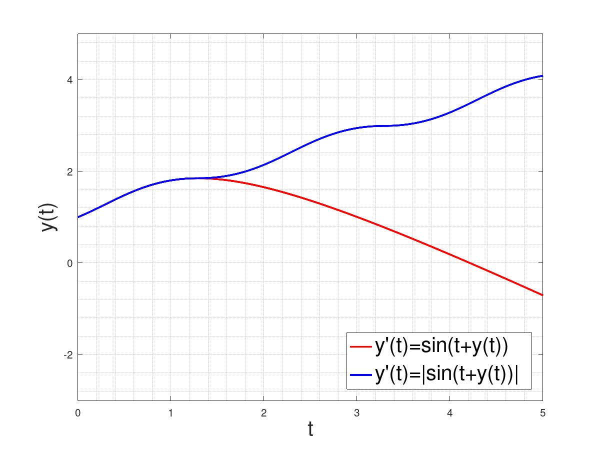
   Figure 1: The solution of $y^{\prime}(t)=\sin(t+y(t))$ in red versus that of $y^{\prime}(t)=\lvert\thinspace{\sin(t+y(t))}\thinspace\rvert$ in blue, over the domain $[0,5]$. Around $t=1.295$, the two solutions diverge.

In our experiments, we consider a parameter depth, which denotes how many times the domain $[0,a]$ must been bisected. For instance, when running any of the operators at depth $4$, the domain $[0,a]$ is discretized into $2^{4}=16$ equal sized subintervals. We ran the first-order operator $E^{c}$ of [23] and the second-order Euler operator $E^{2}$ on all of the IVP, and ran the Runge-Kutta operator $E^{\mathrm{R}}$ on the scalar IVP (72) and (73), for a range of depths from $2$ to $16$.

Figure 2 contains three plots related to the IVP (72) with $y^{\prime}(t)=y(t)$:

• The left plot shows that at each depth, the width of the solution obtained from $E^{2}$ is noticeably smaller than the widths obtained from the Runge-Kutta $E^{\mathrm{R}}$ and the first-order operator $E^{c}$.

• The middle plot shows that at equal depths, the second-order and Runge-Kutta methods take more time compared with the first-order method. This is expected due to the overhead of handling derivatives.

• The right plot shows that, in the particular case of the IVP (72), the overall performance of the first-order operator $E^{c}$ is better. In simple terms, by spending the same amount of CPU time, the first-order method provides tighter enclosures of the solution.

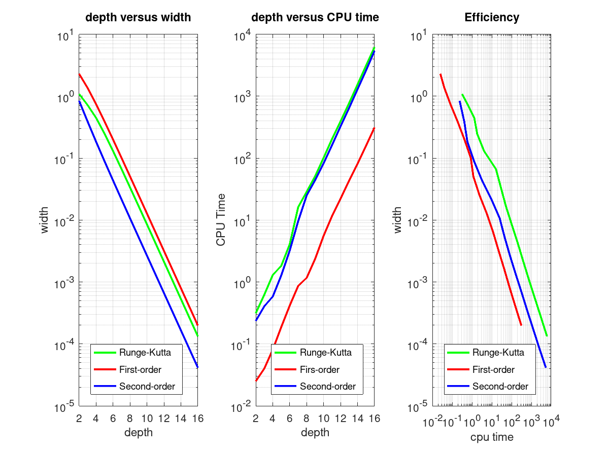
Figure 2: Comparison of the first-order, second-order, and Runge-Kutta Euler methods on the IVP (72), with $y^{\prime}(t)=y(t)$.

Figure 3 contains the plots related to the IVP (73). The right plot demonstrates that at lower depths, the first-order operator $E^{c}$ is the most efficient. Nonetheless, at higher depths, the second-order operator outperforms both the first-order and Runge-Kutta operators due to its superior convergence rate.

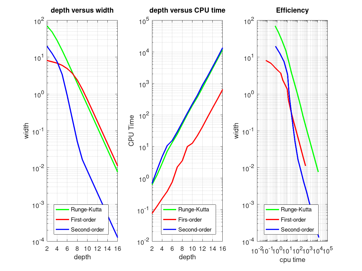
Figure 3: Comparison of the first-order, second-order, and Runge-Kutta Euler methods on the IVP (73), with $y^{\prime}(t)=\cos(y(t))$.

Figure 4 contains the plots related to the IVP (74). As the IVP is converted to a non-scalar one, we may only apply the first-order and second-order operators $E^{c}$ and $E^{2}$, respectively. The left and middle plots have the same quality as those of Figure 2. The right plot, however, shows that, in this case, the second-order method outperforms the first-order Euler method in overall efficiency.

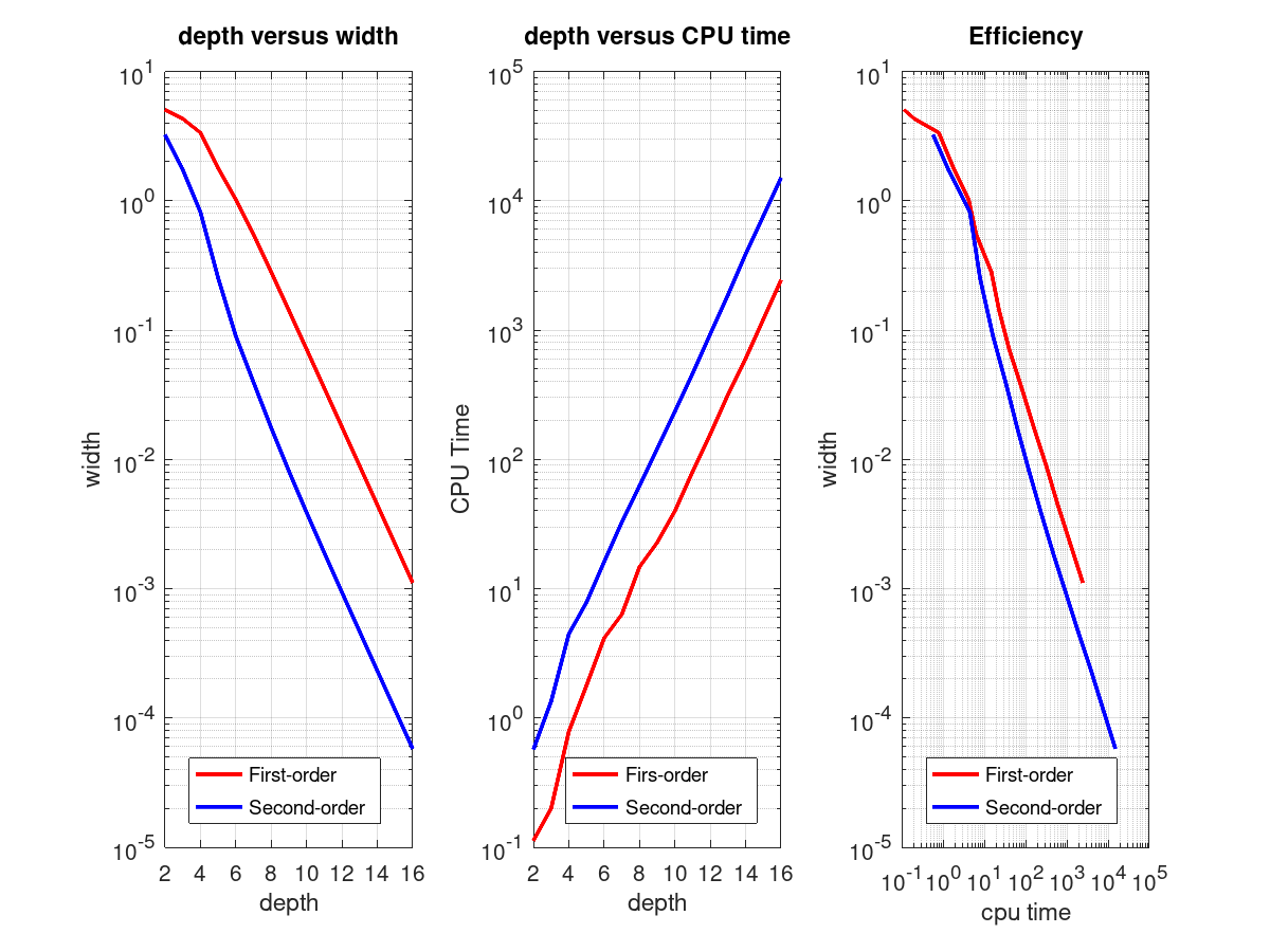
Figure 4: Comparison of the first-order and second-order Euler methods on the IVP (74) with $\hat{y}^{\prime}(t)=10\cos(10t)\hat{y}(t)$.

Figure 5 contains the relevant plots for the IVP (75). As the IVP is converted to a non-scalar one, and the vector field is not continuously differentiable, we may only apply the first-order and second-order operators $E^{c}$ and $E^{2}$, respectively. The middle plot is as expected, but the left and right plots demonstrate the effect of the overhead of handling derivatives in the second-order method. In lower depths, the first-order Euler operator performs better, but as the depth is increased, the faster convergence of the second-order operator makes it overall more efficient.

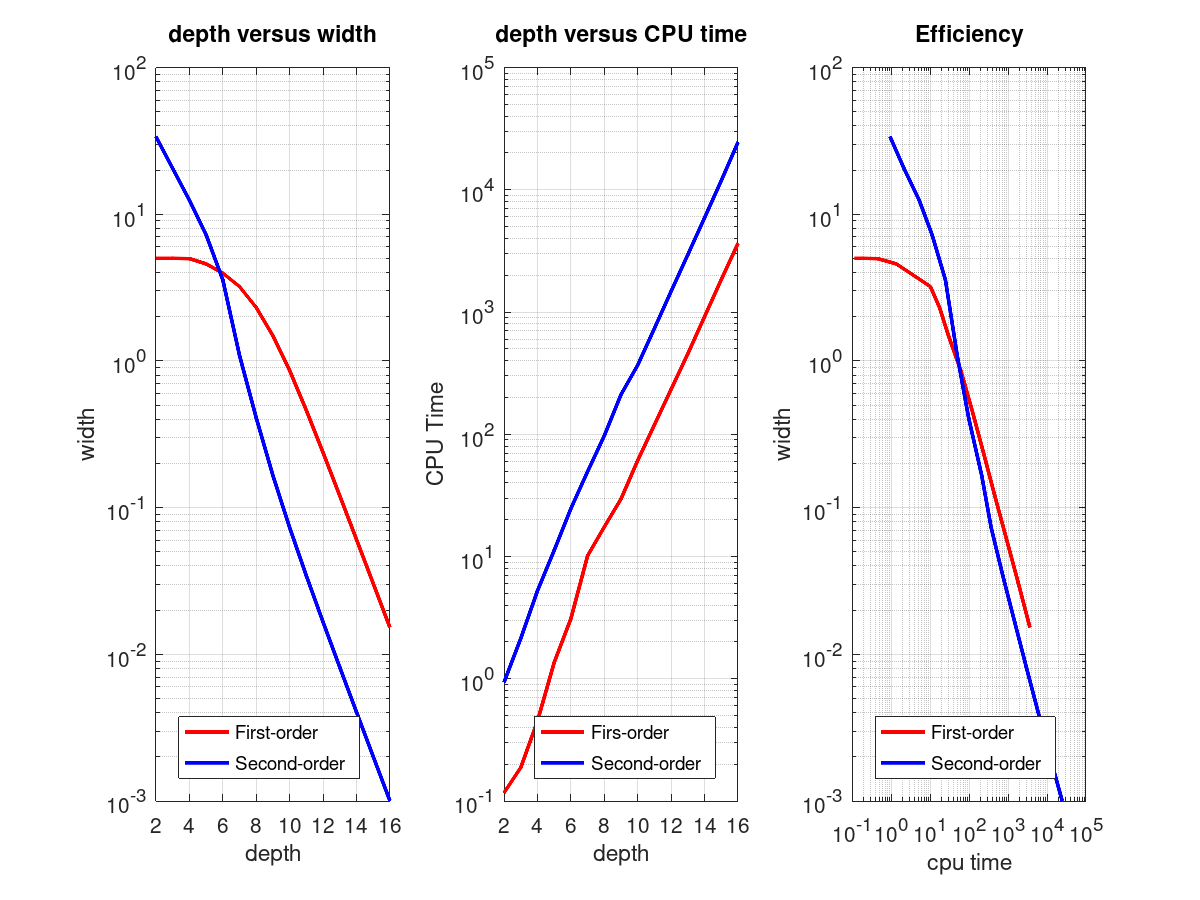
Figure 5: Comparison of the first-order and second-order Euler methods on the IVP (75), with a non-differentiable vector field: $\hat{y}^{\prime}(t)=\lvert\thinspace{\sin(t+\hat{y}(t))}\thinspace\rvert$.

As we have already pointed out in Section 5.3.1, although Theorems 5.21 and 5.22 require the vector field to be continuously differentiable, we conjecture that the second-order convergence is retained over non-differentiable vector fields as well. As a witness to this conjecture, we compare the convergence of the second-order Euler method for solving the IVP (75)–with a non-differentiable vector field—with those obtained from solving IVP (73) and (74), with vector fields that are continuously differentiable. Figure 6 suggests that the convergence has the same order in this case.

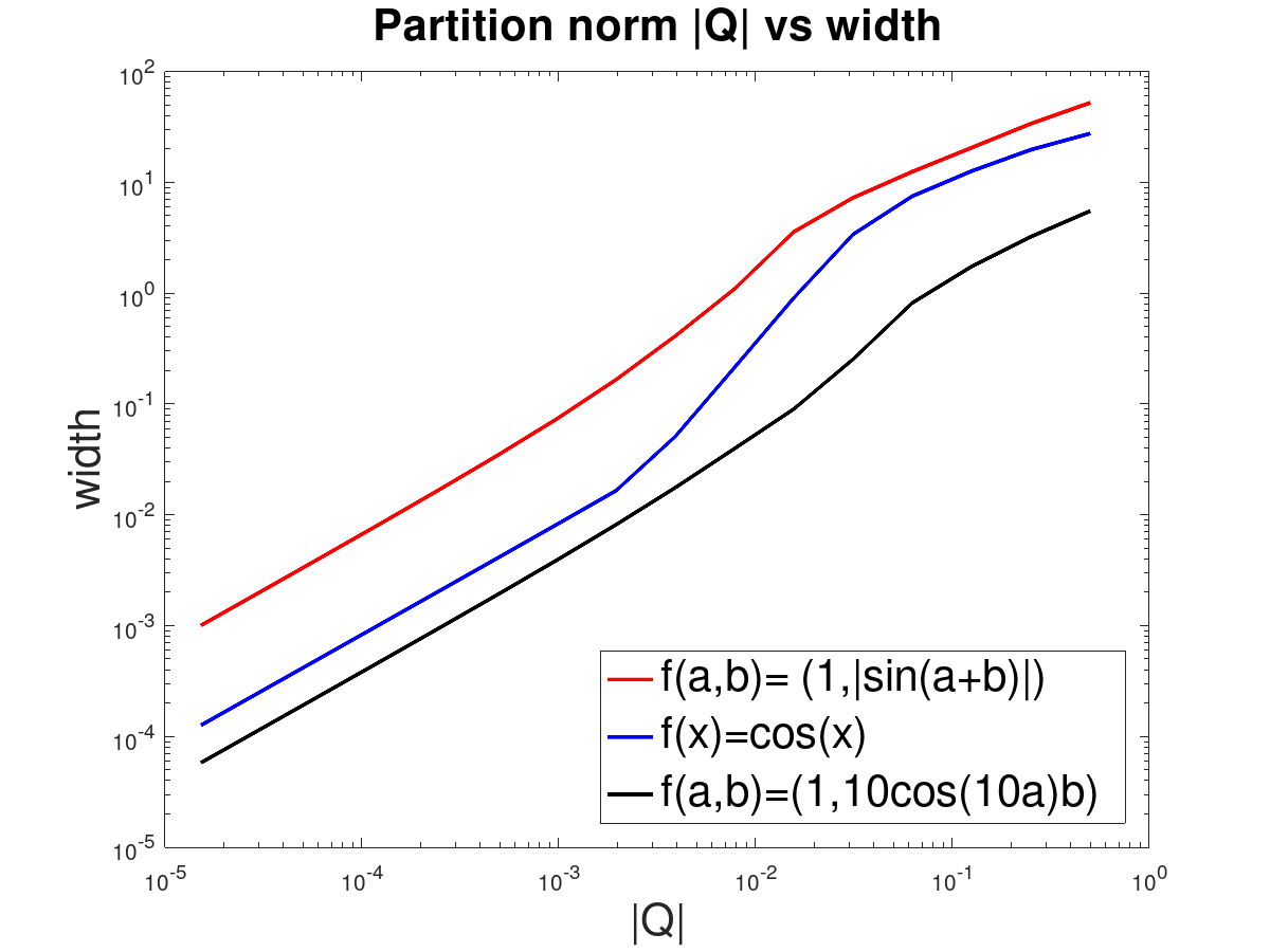
Figure 6: Comparison of the convergence of the second-order Euler method on the IVP (75), with a non-differentiable vector field (in red), and the IVP (73) and (74), with vector fields that are continuously differentiable (in blue and black). The second-order convergence seems to be retained for the IVP (75).

7.1 Static Analysis

The bound (53) (obtained in [20]) and those obtained in the current work (i. e., Corollary 5.20 and Theorem 5.22) make it possible to perform a static convergence analysis. These bounds, however, are usually very conservative, and result in unnecessarily small partition norms for obtaining a required accuracy. In practice, it is more efficient to just run the Euler operators for various depths, in increasing order, until the required accuracy is obtained.

Take the IVP (74) as an example. A static analysis based on the bound (53) would indicate that, in order to obtain $\epsilon>0$ accuracy, one must take the partition norm small enough to satisfy:

$$|Q|\leq\frac{\epsilon}{15(\mathrm{e}^{60}-1)}\leq\frac{\epsilon}{1.72\times 10^{27}}.$$

As an example, according to this estimate, to obtain an accuracy of $\epsilon\leq 10^{-4}$, we must partition $[0,0.1]$ to at least the depth of $100$, resulting in $2^{100}$ subintervals, which is prohibitively large. Instead, we start from a small depth of $2$, and increase the depth until the accuracy is reached. With this approach, the accuracy reaches the target of $10^{-4}$ at depth $16$, in under $30$ seconds on a personal laptop, with an Intel^® Core™ i7-8550U CPU at 1.80GHz and 16GB RAM, under Ubuntu 20.04 LTS environment.

Remark 7.1.

Although we have reported the timing of our experiments and the hardware that has been used, the numbers should be considered only in the context of comparison between the algorithms that we have implemented. The Euler operator $E^{2}$ is second-order, and as such, over IVP with highly smooth vector fields, it may not exhibit the efficiency of the high-order methods such as COSY [5], VNODE [62] or ValEncIA-IVP [64]. On the other hand, our method is superior in its generality as it can provide validated solution of IVP with non-differentiable vector fields as well, while the high-order methods available in the literature invariably require the vector field to be continuously differentiable.

8 Concluding Remarks

The analyses presented in the current article are applicable to any operator that follows the general schema presented in Section 4. Given the superiority of the Euler operator $E^{2}$ over the Runge-Kutta variant $E^{\mathrm{R}}$, one immediate candidate is higher-order extensions of $E^{2}$. In fact, the foundations are in place for such an extension. These include the domain model ${\mathcal{W}}_{\mathcal{D}}$ of the current article, the domain of Lipschitz functions developed in [22], and an extension of the Taylor’s theorem, as presented in [20, Corollary 2.14]. To obtain a full formulation for the $m$-th order variant $E^{m}$ of $E^{2}$, the (non-scalar) differential equation $y^{\prime}=f(y)$ must be differentiated $(m-1)$ times, and the right hand side written solely in terms of the vector field $f$ and its derivatives. This may be done using, e. g., the well-known Faà di Bruno formula [11]. Although of practical importance, this extension will require careful handling of lengthy formulas, and may not require any significant theoretical novelty.

A similar extension may also be considered for higher-order Runge-Kutta methods. Again, the foundation is available, not just based on the domain model of the current paper and that of [22], but also based on the catalogue of validated Runge-Kutta methods available in [47].

We have proved that the operator $E^{2}$ has a second-order convergence when the vector field of the IVP is continuously differentiable. The definition of the operator, however, only requires the vector field to be Lipschitz continuous. One direction for further investigation is convergence analysis of the operator $E^{2}$ under the assumption that the vector field is Lipschitz continuous but not differentiable. As we have demonstrated, there is strong evidence that the rate of convergence is not jeopardized by non-differentiability of the Lipschitz vector field. This is potentially significant because, to the best of our knowledge, all the higher-order validated methods in the literature require the vector field to be at least (once) continuously differentiable.

We presented the construction of a continuous domain for function spaces $[X\to D]$, for any topological space $X$ and bounded-complete continuous domain $D$. When $X$ is core-compact, the DCPO $[X\to D]$ is continuous. Thus, in practice, our general construction may be more relevant when $X$ is not core-compact. We exemplified this claim via the concrete case of differential equation solving with temporal discretization, where the relevant topology is the upper limit topology, which is not core-compact. It will be interesting to see if the construction is useful for other applications as well, e. g., stochastic processes with right-continuous jumps.

Probabilistic power domains have been used previously for analysis of stochastic processes. Specifically, in [15], domain-theoretic models of finite-state discrete stochastic processes have been introduced, while in [7] a more general approach has been taken for continuous time, continuous space stochastic processes. The construction of the current article can be modified for stochastic processes with right-continuous jumps. To be more precise, while the upper limit topology had to be used for temporal discretization in differential equation solving, the suitable topology for analysis of processes with right-continuous jumps is the lower limit topology, which is not core-compact either. Furthermore, while the rational $P$-functions satisfying (28) are left continuous with right limits, in the study of stochastic processes, one must work with the so-called càdlàg functions, which are right-continuous with left limits [6, Chapter 3].

References

• [1] Samson Abramsky and Achim Jung “Domain Theory” In Handbook of Logic in Computer Science 3 Oxford: Clarendon Press, 1994, pp. 1–168
• [2] Götz Alefeld and Günter Mayer “Interval analysis: theory and applications” In Journal of Computational and Applied Mathematics 121.1, 2000, pp. 421–464 DOI: 10.1016/S0377-0427(00)00342-3
• [3] Julien Alexandre dit Sandretto and Alexandre Chapoutot “Validated Explicit and Implicit Runge-Kutta Methods” In Reliable Computing electronic edition 22, 2016
• [4] John Backus “Can Programming Be Liberated from the Von Neumann Style?: A Functional Style and Its Algebra of Programs” In Commun. ACM 21.8 New York, NY, USA: ACM, 1978, pp. 613–641 DOI: 10.1145/359576.359579
• [5] Martin Berz and Kyoko Makino “Verified Integration of ODEs and Flows Using Differential Algebraic Methods on High-Order Taylor Models” In Reliable Computing 4, 1998, pp. 361–369
• [6] Patrick Billingsley “Convergence of Probability Measures” John Wiley & Sons, Inc., 1999
• [7] Paul Bilokon and Abbas Edalat “A Domain-Theoretic Approach to Brownian Motion and General Continuous Stochastic Processes” In Theoretical Computer Science 691, 2017, pp. 10–26 DOI: 10.1016/j.tcs.2017.07.016
• [8] Sylvie Boldo and Guillaume Melquiond “Computer Arithmetic and Formal Proofs: Verifying Floating-point Algorithms with the Coq System” Elsevier, 2017
• [9] Frank H. Clarke “Optimization and Nonsmooth Analysis”, Classics in Applied Mathematics Philadelphia, PA: Society for IndustrialApplied Mathematics, 1990
• [10] Frank H. Clarke, Yuri S. Ledyaev, Ron J. Stern and Peter R. Wolenski “Nonsmooth Analysis and Control Theory” Springer, 1998
• [11] Gregory M. Constantine and Thomas H. Savits “A Multivariate Faa di Bruno Formula with Applications” In Trans. Amer. Math. Soc. 348, 1996, pp. 503–520
• [12] Pietro Di Gianantonio “Real Number Computability and Domain Theory” In Information and Computation 127.1, 1996, pp. 11–25
• [13] Pietro Di Gianantonio and Abbas Edalat “A Language for Differentiable Functions” In Foundations of Software Science and Computation Structures Berlin, Heidelberg: Springer Berlin Heidelberg, 2013, pp. 337–352 DOI: 10.1007/978-3-642-37075-5˙22
• [14] Abbas Edalat “A Continuous Derivative for Real-Valued Functions” In New Computational Paradigms: Changing Conceptions of What is Computable New York, NY: Springer, 2008, pp. 493–519
• [15] Abbas Edalat “Domain Theory in Stochastic Processes” In Proceedings of Tenth Annual IEEE Symposium on Logic in Computer Science, 1995, pp. 244–254 DOI: 10.1109/LICS.1995.523260
• [16] Abbas Edalat “Domains for Computation in Mathematics, Physics and Exact Real Arithmetic” In Bull. Symbolic Logic 3.4 Association for Symbolic Logic, 1997, pp. 401–452
• [17] Abbas Edalat “Dynamical Systems, Measures and Fractals via Domain Theory” In Information and Computation 120.1, 1995, pp. 32–48
• [18] Abbas Edalat “Smooth Approximation of Lipschitz Maps and Their Subgradients” In Journal of the ACM 69.1, 2021, pp. 1–32 DOI: 10.1145/3481805
• [19] Abbas Edalat and Martın Hötzel Escardó “Integration in Real PCF” In Information and Computation 160.1-2, 2000, pp. 128–166
• [20] Abbas Edalat, Amin Farjudian, Mina Mohammadian and Dirk Pattinson “Domain Theoretic Second-Order Euler’s Method for Solving Initial Value Problems” The 36th Mathematical Foundations of Programming Semantics Conference, 2020 (MFPS 2020), Paris, France In Electr. Notes in Theoret. Comp. Sci. 352, 2020, pp. 105–128
• [21] Abbas Edalat and André Lieutier “Domain Theory and Differential Calculus (Functions of One Variable)” In Mathematical. Structures in Comp. Sci. 14.6 USA: Cambridge University Press, 2004, pp. 771–802
• [22] Abbas Edalat, André Lieutier and Dirk Pattinson “A Computational Model for Multi-Variable Differential Calculus” In Information and Computation 224, 2013, pp. 23–45
• [23] Abbas Edalat and Dirk Pattinson “A Domain Theoretic Account of Euler’s Method for Solving Initial Value Problems” In PARA 3732, Lecture Notes in Computer Science, 2006, pp. 112–121
• [24] Abbas Edalat and Dirk Pattinson “A Domain-Theoretic Account of Picard’s Theorem” In LMS Journal of Computation and Mathematics 10, 2007, pp. 83–118
• [25] Abbas Edalat and Dirk Pattinson “Denotational Semantics of Hybrid Automata” In The Journal of Logic and Algebraic Programming 73.1 Elsevier, 2007, pp. 3–21
• [26] Abbas Edalat and Dirk Pattinson “Inverse and Implicit Functions in Domain Theory” In Proceedings. 20th Annual IEEE Symposium on Logic in Computer Science IEEE Computer Society, 2005, pp. 417–426
• [27] Abbas Edalat and Philipp Sünderhauf “A Domain Theoretic Approach to Computability on the Real Line” In Theoretical Computer Science 210, 1999, pp. 73–98
• [28] Thomas Erker, Martín Hötzel Escardó and Klaus Keimel “The Way-Below Relation of Function Spaces Over Semantic Domains” In Topology and its Applications 89.1, 1998, pp. 61–74 DOI: 10.1016/S0166-8641(97)00226-5
• [29] Martin Hötzel Escardó “PCF Extended with Real Numbers” In Theoretical Computer Science 162, 1996, pp. 79–115
• [30] Amin Farjudian “Shrad: A Language for Sequential Real Number Computation” In Theory Comput. Syst. 41.1, 2007, pp. 49–105
• [31] Amin Farjudian and Michal Konečný “Time Complexity and Convergence Analysis of Domain Theoretic Picard Method” In Proceedings of WoLLIC ’08 5110, Lecture Notes in Artificial Intelligence Springer, 2008, pp. 149–163
• [32] Gerhard Gierz et al. “A Compendium of Continuous Lattices” Springer, 1980
• [33] Gerhard Gierz et al. “Continuous Lattices and Domains” 93, Encycloedia of Mathematics and its Applications Cambridge University Press, 2003
• [34] Jean Goubault-Larrecq “Non-Hausdorff topology and domain theory” Cambridge University Press, 2013
• [35] Eldon Hansen and G. William Walster “Global Optimization Using Interval Analysis”, Pure and Applied Mathematics Series Marcel Dekker, 2004
• [36] Peter Hertling “Clarke’s Generalized Gradient and Edalat’s $L$-derivative” In Journal of Logic & Analysis 9, 2017, pp. 1–21
• [37] Nicholas J. Higham “Accuracy and Stability of Numerical Algorithms” Philadelphia, PA, USA: Society for IndustrialApplied Mathematics, 2002
• [38] Milan Hladík, David Daney and Elias P. Tsigaridas “An algorithm for addressing the real interval eigenvalue problem” In Journal of Computational and Applied Mathematics 235.8, 2011, pp. 2715–2730 DOI: 10.1016/j.cam.2010.11.022
• [39] Tomasz Hoffmann, Andrzej Marciniak and Barbara Szyszka “Interval Versions of Central-Difference Method for Solving the Poisson Equation in Proper and Directed Interval Arithmetic” In Foundations of Computing and Decision Sciences 38.3, 2013, pp. 193–206 DOI: 10.2478/fcds-2013-0009
• [40] Zhenjiang Hu, John Hughes and Meng Wang “How functional programming mattered” In National Science Review 2.3, 2015, pp. 349–370 DOI: 10.1093/nsr/nwv042
• [41] J. Hughes “Why Functional Programming Matters” In The Computer Journal 32.2, 1989, pp. 98–107 DOI: 10.1093/comjnl/32.2.98
• [42] Arieh Iserles “A First Course in the Numerical Analysis of Differential Equations”, Cambridge Texts in Applied Mathematics Cambridge University Press, 2009
• [43] Akitoshi Kawamura “Lipschitz Continuous Ordinary Differential Equations Are Polynomial-Space Complete” In CCC ’09: 24th Annual IEEE Conference on Computational Complexity, 2009, pp. 149–160
• [44] Klaus Keimel “Domain Theory its Ramifications and Interactions” The Seventh International Symposium on Domain Theory and Its Applications (ISDT) In Electronic Notes in Theoretical Computer Science 333.Supplement C, 2017, pp. 3–16
• [45] Michal Konečný, Jan Duracz, Amin Farjudian and Walid Taha “Picard Method for Enclosing ODEs with Uncertain Initial Values” In Proceedings of the Eleventh International Conference on Computability and Complexity in Analysis (CCA 2014), 2014, pp. 41–42 Technische Universität Darmstadt, Germany
• [46] John Denholm Lambert “Numerical Methods for Ordinary Differential Systems: The Initial Value Problem” John WileySons, 1991
• [47] Andrzej Marciniak “Selected Interval Methods for Solving the Initial Value Problem” http://www.cs.put.poznan.pl/amarciniak/IMforIVP-book/IMforIVP.pdf Poznan: Publishing House of Poznan University of Technology, 2009
• [48] Andrzej Marciniak and Barbara Szyszka “Interval Runge-Kutta Methods with Variable Step Sizes” In Computational Methods in Science and Technology 25.1, 2019, pp. 17–29 DOI: 10.12921/cmst.2019.0000006
• [49] Valérie Ménissier-Morain “Arbitrary Precision Real Arithmetic: Design and Algorithms” In Journal of Logic and Algebraic Programming 64.1, 2005, pp. 13–39
• [50] Richard Miller and Anthony Michel “Ordinary Differential Equations” Academic Press, 1982
• [51] Atsushi Minamihata, Takeshi Ogita, Siegfried M. Rump and Shin’ichi Oishi “Modified error bounds for approximate solutions of dense linear systems” In Journal of Computational and Applied Mathematics 369, 2020, pp. 112546 DOI: 10.1016/j.cam.2019.112546
• [52] Eugenio Moggi, Amin Farjudian, Adam Duracz and Walid Taha “Safe & Robust Reachability Analysis of Hybrid Systems” In Theoretical Computer Science 747, 2018, pp. 75–99
• [53] Eugenio Moggi, Amin Farjudian and Walid Taha “System Analysis and Robustness” In Models, Mindsets, Meta: The What, the How, and the Why Not? Essays Dedicated to Bernhard Steffen on the Occasion of His 60th Birthday Springer International Publishing, 2019, pp. 36–44
• [54] Eugenio Moggi, Amin Farjudian and Walid Taha “System Analysis and Robustness” In Proceedings of the 20th Italian Conference on Theoretical Computer Science, ICTCS 2019, Como, Italy, September 9-11, 2019, 2019, pp. 1–7 URL: http://ceur-ws.org/Vol-2504/paper1.pdf
• [55] Ramon E. Moore “Automatic Error Analysis in Digital Computation”, 1959
• [56] Ramon E. Moore “Interval Analysis” Englewood Cliffs, New Jersey, USA: Prentice-Hall, 1966
• [57] Ramon E Moore and Michael J Cloud “Computational Functional Analysis” Elsevier, 2007
• [58] Ramon E. Moore and Sandie Turner Jones “Safe Starting Regions for Iterative Methods” In SIAM Journal on Numerical Analysis 14, 1977, pp. 1051–1065
• [59] Ramon E. Moore, R. Baker Kearfott and Michael J. Cloud “Introduction to Interval Analysis” Philadelphia, PA, USA: Society for IndustrialApplied Mathematics, 2009
• [60] Jean-Michel Muller “Arithmétique des ordinateurs” Masson, 1989
• [61] Norbert Müller and Bernd Moiske “Solving Initial Value Problems in Polynomial Time” In Proc. 22 JAIIO - PANEL ’93, Part 2, 1993, pp. 283–293
• [62] Nedialko S. Nedialkov, Kenneth R. Jackson and John D. Pryce “An Effective High-Order Interval Method for Validating Existence and Uniqueness of the Solution of an IVP for an ODE” In Reliable Computing 7, 2001, pp. 449–465
• [63] Alfio Quarteroni, Riccardo Sacco and Fausto Saleri “Numerical Mathematics” Springer, 2000
• [64] Andreas Rauh, Eberhard P. Hofer and Ekaterina Auer “ValEncIA-IVP: A Comparison with Other Initial Value Problem Solvers” In CD-Proc. of the 12th GAMM-IMACS International Symposium on Scientific Computing, Computer Arithmetic, and Validated Numerics SCAN 2006, Duisburg, Germany, IEEE Computer Society, 2007, pp. 36
• [65] Nathalie Revol and Fabrice Rouillier “Motivations for an Arbitrary Precision Interval Arithmetic and the MPFI Library” In Reliable Computing 11.4, 2005, pp. 275–290
• [66] Siegfried M. Rump “Addendum to ‘On recurrences converging to the wrong limit in finite precision and some new examples”’ In Electronic Transactions on Numerical Analysis 52, 2020, pp. 571–575 DOI: 10.1553/etna˙vol52s571
• [67] Siegfried M. Rump “On recurrences converging to the wrong limit in finite precision and some new examples” In Electronic Transactions on Numerical Analysis 52, 2020, pp. 358–369 DOI: 10.1553/etna˙vol52s358
• [68] Hartmut Schwandt “Almost Globally Convergent Interval Methods for Discretizations of Nonlinear Elliptic Partial Differential Equations” In SIAM Journal on Numerical Analysis 23.2, 1986, pp. 304–324 DOI: 10.1137/0723022
• [69] Dana Scott “Outline of a Mathematical Theory of Computation” In Proceedings of the Fourth Annual Princeton Conference on Information Sciences and Systems, 1970, pp. 169–176
• [70] Dana Scott “Outline of a Mathematical Theory of Computation” Oxford University Computing Laboratory, Programming Research Group Oxford, 1970
• [71] Michael B. Smyth “Effectively Given Domains” In Theoretical Computer Science 5, 1977, pp. 257–274
• [72] RH Sorgenfrey “On the topological product of paracompact spaces” In Bulletin of the American Mathematical Society 53.6 American Mathematical Society, 1947, pp. 631–632
• [73] T. Sunaga “Theory of an interval algebra and its application to numerical analysis” In RAAG Memoirs 2, 1958, pp. 29–46
• [74] Alfred Tarski “A Decision Method for Elementary Algebra and Geometry” In Quantifier Elimination and Cylindrical Algebraic Decomposition Vienna: Springer Vienna, 1998, pp. 24–84 DOI: 10.1007/978-3-7091-9459-1˙3
• [75] Gerald Teschl “Ordinary Differential Equations and Dynamical Systems”, Graduate studies in mathematics American Mathematical Society, 2012
• [76] Hoffmann Tomasz and Andrzej Marciniak “Solving the generalized Poisson equation in proper and directed interval arithmetic” In CMST 22.4 PSNC, Poznan SupercomputingNetworking Center, 2016, pp. 225–232
• [77] Warwick Tucker “Validated Numerics: A Short Introduction to Rigorous Computations” Princeton University Press, 2011
• [78] Shiqi Wang, Kexin Pei, Justin Whitehouse, Junfeng Yang and Suman Jana “Formal Security Analysis of Neural Networks Using Symbolic Intervals” In Proceedings of the 27th USENIX Conference on Security Symposium, SEC’18 Baltimore, MD, USA: USENIX Association, 2018, pp. 1599–1614
• [79] Mieczyslaw Warmus “Calculus of Approximations” In Bulletin de l’Académie Polonaise des Sciences, Cl. III 4.5, 1956, pp. 253–259
• [80] Klaus Weihrauch “Computable Analysis, An Introduction” Springer, 2000
• [81] Taro Yoshizawa and Kyuzo Hayashi “On the Uniqueness of Solutions of a System of Ordinary Differential Equations” In Memoirs of the College of Science, University of Kyoto. Ser. A, Mathematics 26.1, 1950, pp. 19–29
• [82] Can Zhou, Razin A. Shaikh, Yiran Li and Amin Farjudian “A domain-theoretic framework for robustness analysis of neural networks” In Mathematical Structures in Computer Science 33.2 Cambridge University Press, 2023, pp. 68–105 DOI: 10.1017/S0960129523000142