Particle-photon radiative interactions and thermalization

Abstract

We analyze the statistical properties of radiative transitions for a molecular system possessing discrete, equally spaced, energy levels, interacting with thermal radiation at constant temperature. A radiative fluctuation-dissipation theorem is derived and the particle velocity distribution analyzed. It is shown analytically that, neglecting molecular collisions, the velocity distribution function cannot be Gaussian, as the equilibrium value for the kurtosis $\kappa$ is different from $\kappa=3$. A Maxwellian velocity distribution can be recovered in the limit of small radiative friction.

I Introduction

One of the main contribution of quantum mechanics is the discovery that molecules do possess an internal energy structure, owing to which they radiatively interact with the electromagnetic field via emission and absorption of energy quanta (photons) quantum1 ; quantum2 . This phenomenon has a deep influence on the statistical and thermodynamic properties of molecular systems, as shown by Einstein, Debye and many others thermo1 ; thermo2 , both as regards equilibrium and non-equilibrium properties. The theory of the specific heats of molecules (for instance diatomic molecules) diatomic and of solids solid1 cannot be correctly framed without considering the quantum description of the excitations of the internal mechanical degrees of freedom.

The electromagnetic field, described by the system of the Maxwell equations, is responsible for mechanical actions in its interaction with material bodies (massive matter) due to momentum exchange (radiation pressure). This is well known since Maxwell’s times, and this currently finds important fields of applications in the study of condensed matter, in microtechnology and microfluidics, in biology, as it is possible to manipulate mechanically micrometric particles, cells, and molecules through the use of light beams (optical tweezers) tweezers1 ; tweezers2 ; tweezers3 , focus particles at a given spatial location (optical traps) traps , or induce extreme thermal conditions in molecular assemblies via optical interactions (laser cooling techniques) cooling1 ; cooling2 ; cooling3 .

Nevertheless, the most remarkable effects, as regards thermodynamic properties, is that the momentum exchange between matter and radiation (recoil effect) is the physical mechanism leading to thermalization. As shown by Einstein einstein1916 , considering exclusively radiative interactions between a molecular gas of identical molecules of mass $m$, and thermal radiation at constant temperature $T$, the squared variance of the particle velocity entries $\langle v_{i}^{2}\rangle$, $i=1,2,3$, (since $\langle v_{i}\rangle=0$) equals at equilibrium the Maxwellian result thermo2

$$\langle v_{i}^{2}\rangle=\frac{k_{B}\,T}{m}$$ (1)

where $k_{B}$ is the Boltzmann constant.

In this article we analyze the statistical properties of this interaction, formulating the problem in the form of a stochastic process over the increments of a Poisson counting process, applying the formalism recently proposed in PG1 for stochastic chemical reactions. Extending the analysis to momentum transfer, we derive a radiative fluctuation-dissipation relation and the statistical properties of the particle velocities at equilibrium. Throughout this article we consider exclusively radiative interactions as regards particle momentum dynamics, deliberately neglecting the influence of particle-particle collisions. This choice has been made in order to enucleate and clarify the effects of the momentum exchange between particles and radiation on the statistical mechanical properties of a particle gas. Despite the fact that radiative interactions provide the physical mechanism for thermalization, in the meaning of eq. (1), the resulting velocity distributions deviate from the Maxwellian, and a Gaussian shape is recovered in the limit of small radiative friction.

The article is organized as follows. Section II briefly introduces the problems and reviews the basic conservation principles that apply, and the meaning of Einstein’s result einstein1916 . Section III develops the stochastic equations for the occupation numbers of the internal energy levels of a molecular system interacting with a given number of photons. We adopt the approximation of closed system discussed in lami1985 , deriving the equilibrium properties. Section IV addresses the thermalization problem, i.e., the statistics of the momentum exchange between a particle gas and thermal radiation at constant temperature $T$. A new stochastic formulation of the particle equations of motion over the increments of a Poisson process is developed (the Appendix addresses some technicalities associated with this class of equations). A radiative fluctuation-dissipation theorem is formulated and the functional form of the velocity distribution function thoroughly considered in Section VII, showing its generic deviation from the Maxwellian behavior.

II Radiative interactions

The interaction between a molecular system with radiation develops through: (i) radiative processes of emission and absorption of radiation, (ii) photon-molecule scattering, (iii) interactions with the zero-point energy field zpf1 ; zpf2 . According to the analysis developed in einstein1916 , we neglect scattering processes, and the interactions with zero-point fluctuations, focusing exclusively on the effects of radiative transitions. Consider the transition of a quantum system (molecule) from the energy level $E_{1}$ to the energy level $E_{2}$ due to absorption of an energy quantum of frequency $\nu$, with

$$E_{2}-E_{1}=h\,\nu$$ (2)

where $h$ is the Planck constant. This elementary event fulfils the fundamental principles of conservation of energy and momentum. Let ${\bf v}_{1}$ and ${\bf v}_{2}$ be the velocities of the molecule before and after the radiative interaction with the photon (in the present case an absorption event). Since a photon of energy $h\,\nu$ possesses a momentum ${\bf p}_{\phi}$ given by

$${\bf p}_{\phi}=\frac{h\,\nu}{c}\,{\bf n}$$ (3)

where $c$ is the speed of light in vacuo and ${\bf n}$ the unit vector in the direction of propagation, in the low-velocity limit, (so that relativistic corrections can be neglected), the energy balance reads

$$E_{1}+\frac{1}{2}m\,|{\bf v}_{1}|^{2}+h\,\nu=E_{2}+\frac{1}{2}\,m\,|{\bf v}_{2}|^{2}$$ (4)

where $m$ is the mass of the molecule, and the momentum balance takes the form

$$m\,{\bf v}_{1}+\frac{h\,\nu}{c}\,{\bf n}=m\,{\bf v}_{2}$$ (5)

As the kinetic energy contributions are negligible, since using eq. (5), eq. (4) can be expressed as

$$E_{1}+h\,\nu\,(1-\varepsilon)=E_{2}\,,\qquad\varepsilon=\frac{2\,{\bf v}\cdot{\bf n}}{c}+\frac{h\,\nu}{m\,c^{2}}$$ (6)

and $\varepsilon$ is small in the non-relativistic limit ($v/c\ll 1$), and for generic molecular systems ($h\nu/mc^{2}\ll 1$), eq. (4) can be simplified as

$$E_{1}+h\,\nu=E_{2}$$ (7)

As observed in einstein1916 , the radiative interactions, once considered in the reference frame of the moving particle, should account for relativistic corrections, specifically related to the property that the equilibrium spectral density of the radiation (the Planck distribution) is not Lorentz covariant. Once expressed in the reference frame of the molecule involved in the interaction, a dissipartive term , proportional to the ratio ${\bf v}_{1}/c$ arises in the momentum balance, so that eq. (5) should be substituted by a dissipative dynamics, containing a friction term, the occurrence of which provides the equilibrium result eq. (1), see also thermo2 ; milonni . In the remainder we take this result for given, leaving to a future work a thorough and comprehensive discussion on the validity of momentum conservation in radiative processes.

III Thermalization of internal quantum states

Consider a system of identical molecules interacting with radiation through emission and absorption of energy quanta. For simplifying the analysis, the following assumptions are made:

• the molecules are characterized by a countable number of equally spaced energy levels $E_{k}$, with $E_{k+1}>E_{k}$, $k=0,1,\dots$, and

  $$E_{k+1}-E_{k}=E_{\delta}=h\,\nu$$ (8)

• the molecules interact with a photon gas at thermal equilibrium with temperature $T$;

• the system is closed and isolated, both as regards molecules and photons.

The latter assumption simplifies the analysis but does not alter the physics of the problem and the results obtained at equilibrium.

Let $p_{k}(t)$ be the number density in the occupation of the $k$-level at time $t$, $p_{k}^{0}$ its initial value at time $t=0$, $q(t)$ the density of photons at the resonant frequency $\nu$, and $q^{0}$ its initial value. Mass conservation implies that

$$\sum_{k=0}^{\infty}p_{k}(t)=\sum_{k=0}^{\infty}p_{k}^{0}=P_{\rm tot}$$ (9)

As the system is supposed to be isolated, i.e. closed with respect to radiation, the principle of conservation of the “virtual photon number” applies, dictating that,

$$q(t)+\sum_{k=1}^{\infty}k\,p_{h}(t)=q^{0}+\sum_{k=0}^{\infty}k\,p_{k}^{0}$$ (10)

The interaction of the molecules with the photon gas implies the emission/absorption of radiation, where the emission process can be either a spontaneous or a stimulated transition, i.e. induced by a collision with an incoming photon. Therefore, if $\lambda$ is the emission rate, we have

$$\lambda=\lambda_{s}+\lambda_{0}\,q(t)$$ (11)

while the absorption rate $\mu$ is given by

$$\mu=\mu_{0}\,q(t)$$ (12)

As shown by Einstein einstein1916 , the specific rate of absorption and stimulated emission should be equal, i.e.,

$$\mu_{0}=\lambda_{0}$$ (13)

Consider for simplicity transition processes betwen nearest nighbouring energy level. The inclusion of higher-order transitions does not add any new physics, making solely the notation more complicated and lengthy. The balance equations for this process read

$$\frac{dp_{k}(t)}{dt} = -\left[(\lambda_{s}+\lambda_{0}q(t))\,\eta_{k}+\lambda_{0}\,q(t)\right]\,p_{k}(t)$$ (14)

$$+ (\lambda_{s}+\lambda_{0}\,q(t))\,p_{k+1}(t)+\lambda_{0}\,q(t)\,p_{k-1}(t)$$

$k=0,1,\dots$, where $\eta_{0}=0$, $\eta_{k}=1$ for $k=1,2,\dots$, and $p_{-1}=0$, and

$$\frac{dq(t)}{dt}=(\lambda_{s}+\lambda_{0}\,q(t))\sum_{k=1}^{\infty}p_{k}(t)-\lambda_{0}\,q(t)\sum_{k=0}^{\infty}p_{k}(t)$$ (15)

In a stochastic representation of the process, let $N_{k}(t)$ be the number of molecules in the $k$-th level, and $N^{q}(t)$ the photon number. If $N_{g}$ is the granularity number chosen PG1 , $\sum_{k=0}^{\infty}N_{k}(0)=N_{g}$, the relations between $N_{k}(t)$ and $p_{k}(t)$ and between $q(t)$ and $N^{q}(t)$ are expressed by

$$p_{k}(t)=P_{\rm tot}\,\frac{N_{k}(t)}{N_{g}}\,,\qquad q(t)=P_{\rm tot}\,\frac{N^{q}(t)}{N_{g}}$$ (16)

Expressed in terms of $N_{k}(t)$, $N^{q}(t)$, the balance equations (14)-(15) thus become

$$\frac{dN_{k}(t)}{dt} = -\left[(\widetilde{\lambda}_{s}+\widetilde{\lambda}_{0}N^{q}(t))\,\eta_{k}+\widetilde{\lambda}_{0}\,N^{q}(t)\right]\,N_{k}(t)$$

$$+ (\widetilde{\lambda}_{s}+\widetilde{\lambda}_{0}\,N^{q}(t))\,N_{k+1}(t)+\widetilde{\lambda}_{0}\,N^{q}(t)\,N_{k-1}(t)$$

$$\frac{dN^{q}(t)}{dt} = (\widetilde{\lambda}_{s}+\widetilde{\lambda}_{0}\,N^{q}(t))\sum_{k=1}^{\infty}N_{k}(t)-\widetilde{\lambda}_{0}\,N^{q}(t)\sum_{k=0}^{\infty}N_{k}(t)$$

with

$$\widetilde{\lambda}_{s}=\lambda_{s}\,,\qquad\widetilde{\lambda}_{0}=\lambda_{0}\,\frac{P_{\rm tot}}{N_{g}}$$ (18)

A stochastic Markovian dynamics follows from eqs. (LABEL:eq_trr15)-(18), applying the formalism developed in PG1 , by considering as stochastic variables the energy state of each molecule and $N^{q}(t)$. Let $\sigma_{\alpha}(t)=0,1,\dots$ be the energy state of the $\alpha$-th molecule at time $t$, $h=1,\dots,N_{g}$. The evolution of $\{\sigma_{\alpha}(t)\}_{\alpha=1}^{N_{g}}$ follows the Markovian dynamics,

$$\frac{d\sigma_{\alpha}(t)}{dt}=-\eta_{\sigma_{\alpha}(t)}\frac{d\chi_{\alpha}^{(e)}(t,\widetilde{\lambda}_{s}+\widetilde{\lambda}_{0}\,N^{q}(t))}{dt}+\frac{d\chi_{\alpha}^{(a)}(t,\widetilde{\lambda}_{0}\,N^{q}(t))}{dt}$$ (19)

while

$$\frac{dN^{q}(t)}{dt} = \sum_{\alpha=1}^{N_{g}}\,\eta_{\sigma_{\alpha}(t)}\,\frac{d\chi_{\alpha}^{(e)}(t,\widetilde{\lambda}_{s}+\widetilde{\lambda}_{0}\,N^{q}(t))}{dt}$$ (20)

$$- \sum_{\alpha=1}^{N_{g}}\frac{d\chi_{\alpha}^{(a)}(t,\widetilde{\lambda}_{0}\,N^{q}(t))}{dt}$$

$\{\chi_{\alpha}^{(e)}(t,\widetilde{\lambda}_{s}+\widetilde{\lambda}_{0}\,N^{q}(t))\}_{\alpha=1}^{N_{g}}$ and $\{\chi_{\alpha}^{(a)}(t,\widetilde{\lambda}_{0}\,N^{q}(t))\}_{\alpha=1}^{N_{g}}$ being two families of $N_{g}$ independent Poisson counting processes, mutually independent of each other, associated with the emission and absorption events of the $\alpha$-th molecules. Observe that the transition rates of these processes depend explictly on the photon number $N^{q}(t)$.

Given $\{\sigma_{\alpha}(t)\}_{\alpha=1}^{N_{g}}$, the occupation number $N_{k}(t)$ of the $k$-th energy level is given by

$$N_{k}(t)=\sum_{\alpha=1}^{N_{g}}\delta_{k,\sigma_{\alpha}(t)}$$ (21)

where $\delta_{k,\sigma_{\alpha}}$ are the Kronecker symbols, so that $\delta_{k,\sigma_{\alpha}(t)}=1$ if $\sigma_{\alpha}(t)=h$, and zero otherwise.

Consider the equilibrium properties of this system, indicating with $p_{k}^{*}$ and $q^{*}$ the equilibrium values. Eq. (14) for $k=0$ at steady state becomes

$$-\lambda_{0}\,q^{*}\,p_{0}^{*}+(\lambda_{s}+\lambda_{0}\,q^{*})\,p_{1}^{*}=0$$ (22)

so that

$$p_{1}^{*}=\frac{\lambda_{0}\,q^{*}}{\lambda_{s}+\lambda_{0}\,q^{*}}\,p_{0}^{*}$$ (23)

An analogous relation applies for generic $k=1,2,\dots$, namely

$$p_{k+1}^{*}=\frac{\lambda_{0}\,q^{*}}{\lambda_{s}+\lambda_{0}\,q^{*}}\,p_{k}^{*}$$ (24)

Therefore, as expected, the equilibrium distribution of level occupation is given by

$$p_{h}=C\,\left(\frac{\lambda_{0}\,q^{*}}{\lambda_{s}+\lambda_{0}\,q^{*}}\right)^{h}=C\,\exp\left[-h\,\log\left(\frac{\lambda_{s}+\lambda_{0}\,q^{*}}{\lambda_{0}\,q^{*}}\right)\right]$$ (25)

It is a discrete Boltzmann distribution, where the term $\log((\lambda_{s}+\lambda_{0}\,q^{*})/\lambda_{0}\,q^{*})$ can be identified with the Boltzmann factor $E_{\delta}/k_{B}\,T$,

$$\frac{E_{\delta}}{k_{B}\,T}=\log\left(\frac{\lambda_{s}+\lambda_{0}\,q^{*}}{\lambda_{0}\,q^{*}}\right)$$ (26)

and this provides an alternative definition of equilibrium temperature $T$ based on radiative interactions

$$T=\frac{E_{\delta}}{k_{B}}\frac{1}{\log\left(\frac{\lambda_{s}+\lambda_{0}\,q^{*}}{\lambda_{0}\,q^{*}}\right)}$$ (27)

From eq. (27), temperature is uniquely specified, once the equilibrium photon density $q^{*}$ is given. Consequently for radiative processes the equilibrium temperature is one-to-one with the steady-state value of the photon density $q^{*}$. Two limit cases can be considered. For $\lambda_{s}\gg\lambda_{0}\,q^{*}$, i.e. for low photon densities, eq. (26) simplifies as

$$\log\left(\frac{\lambda_{s}}{\lambda_{0}\,q^{*}}\right)=\frac{E_{\delta}}{k_{B}\,T}\,,\quad\Rightarrow\quad q^{*}=\frac{\lambda_{s}}{\lambda_{0}}\,e^{-h\,\nu/k_{B}\,T}$$ (28)

In the opposite case, $\lambda_{s}\ll\lambda_{0}\,q^{*}$, i.e., in the high photon-density limit,

$$\log\left(1+\frac{\lambda_{s}}{\lambda_{0}\,q^{*}}\right)\simeq\frac{\lambda_{s}}{\lambda_{0}\,q^{*}}=\frac{E_{\delta}}{k_{B}\,T}$$ (29)

and thus the equilibrium photon density $q^{*}$ is proportional to the temperature $T$

$$q^{*}=\frac{k_{B}\,T}{h\,\nu}\,\frac{\lambda_{s}}{\lambda_{0}}$$ (30)

Next, consider the expression for $q^{*}$. Set $\lambda=\lambda_{s}+\lambda_{0}\,q^{*}$, and $\mu=\lambda_{0}\,q^{*}$, for notational simplicity, and $x=\mu/\lambda<1$, so that the equilibrium occupational distribution can be expressed compactly as $p_{k}^{*}=C\,x^{k}$. The conditions expressed by eqs. (9)-(10) become at equilibrium

$$\sum_{k=0}^{\infty}p_{k}^{*}=P_{\rm tot}$$ (31)

and

$$q^{*}+\sum_{k=1}^{\infty}h\,p_{k}^{*}=q^{0}+\sum_{k=1}^{\infty}p_{k}^{0}=\Phi_{0}$$ (32)

Since $\sum_{k=0}^{\infty}x^{k}=\frac{1}{1-x}$, $\sum_{k=1}^{\infty}k\,x^{k}=\frac{x}{(1-x)^{2}}$, we have for the normalization constant $C$,

$$C=P_{\rm tot}\,(1-x)$$ (33)

and eq. (32) becomes

$$\Phi_{0}-q^{*}=P_{\rm tot}\,\frac{x}{1-x}$$ (34)

that can be explicited with respect to $q^{*}$ to provide

$$q^{*}=\frac{\Phi_{0}}{1+\frac{\lambda_{0}}{\lambda_{s}}\,P_{\rm tot}}$$ (35)

Figure 1 depicts the evolution of $q(t)$ obtained from stochastic simulations at $\lambda_{0}=10^{-3}$ for different values of $\lambda_{s}$. In the simulation we have chosen $P_{\rm tot}=10$, and the initial conditions are $p_{k}^{0}=10\,\delta_{k,10}$, corresponding to an initial population in the 10-th excited state. The stochastic simulation refers to a granularity number $N_{g}=10^{4}$, and $100$ energy levels have been considered.

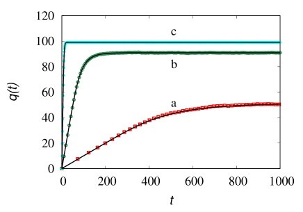
Figure 1: $q(t)$ vs $t$ for different values of $\lambda_{s}$, symbols are the results of stochastic simulations eq. (19)-(20), lines correspond to the solution of the continuous model. Line (a): $\lambda_{s}=0.01$, line (b): $\lambda_{s}=0.1$, line (c): $\lambda_{s}=1$.

The steady-state distributions of the occupation of the energy levels are depicted in figure 2 for the same values of the parameters of figure 1.

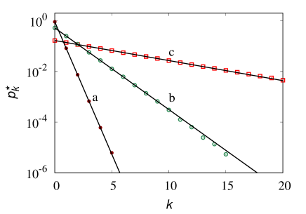
Figure 2: $p_{k}^{*}$ vs $k$ for different values of $\lambda_{s}$, symbols are the results of stochastic simulations eq. (19)-(20), lines correspond to the exponential (Boltzmann) distribution (25) with $q^{*}$ given by eq. (35). Line (a): $\lambda_{s}=0.01$, line (b): $\lambda_{s}=0.1$, line (c): $\lambda_{s}=1$.

From the long-term behavior of $q(t)$, the equilibrium value $q^{*}$ can be obtained. This is depicted in figure 3 as a function of $\lambda_{s}$.

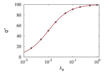
Figure 3: $q^{*}$ vs $\lambda_{s}$ for $\lambda_{0}=10^{-3}$, $P_{\rm tot}=10$, $\phi_{0}=100$. Symbols ($\circ$) are the results of the stochastic simulations (with $N_{g}=10^{4}$), line corresponds to eq. (35).

Finally, figure 4 depicts the value of the scaling exponent $\zeta$ of $p_{k}^{*}$, $p_{k}^{*}=Ce^{-k\zeta}$ obtained for the data of figure 2, compared to the theoretical expression $\zeta=\log((\lambda_{s}+\lambda_{0}\,q^{*})/\lambda_{0}\,q^{*})$, revealing the excellent agreement of the stochastic simulations with the theoretical values.

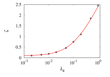
Figure 4: Exponent $\zeta$ vs $\lambda_{s}$ for $\lambda_{0}=10^{-3}$, $P_{\rm tot}=10$, $\phi_{0}=100$. Symbols ($\circ$) are the results of the stochastic simulations (with $N_{g}=10^{4}$), line corresponds to the theoretical expression obtained from the continuous model.

IV Implications of radiative events in the velocity statistics

From the work by Einstein on emission and absorption of radiation einstein1916 it becomes clear that thermalization processes, i.e. the relaxation of a physical system far from equilibrium towards the thermal equilibrium, could be considered as quantum effects driven by emission and absorption of energy quanta.

This is certainly the case of a diluted gas of massive particles (molecules) interacting with thermal radiation (i.e. a photon gas at thermal equilibrium, the statistical properties of which are described by the Planck distribution), in which the following assumptions can be made:

• particle dynamics is characterized by two main interactions: (i) emission and absorption of energy quanta by a particle, and (ii) particle-particle collisions. The assumption of “diluted system” indicates that solely binary collisions are relevant;

• these two processes can be considered as instantaneous events characterized by a Markovian transition structure;

• between two subsequent events (be them particle/photon radiative interactions or particle/particle collisions), the particle motion is purely inertial, i.e. frictionless and in the absence of external or interparticle potentials.

Moreover, relativistic corrections determines the emergence of a dissipative term in the momentum dynamics proportional to the velocity of the molecule. Let us further assume that the particles (molecules) can be represented by a two-level system, where $E_{1}$ and $E_{2}$ are the two energy levels $E_{2}>E_{1}$ and $E_{2}-E_{1}=h\,\nu$.

In this Section we consider exclusively particle/photon radiative interactions and their effects on momentum transfer and velocity statistics, leaving the interplay between radiative processes and mechanical collisions to a subsequent analysis.

Following the assumptions discussed above, the momentum equation for a generic particle, due to the radiative interactions, can be described by means of the stochastic differential equation

$$m\,\frac{d{\bf v}}{dt}=\left(-\eta\,{\bf v}+{\bf b}\right)\,\frac{d\chi(t,\lambda)}{dt}$$ (36)

where $m$ is the particle mass, and ${\bf v}$ its velocity vector. The coefficient $\eta$ is the radiative friction factor, possessing the dimension of a mass. As addressed in Einstein’s work einstein1916 , the radiative friction is an emergent property of the momentum exchange between a molecule and a photon during the radiative process (be it emission or absorption), related to the well-known recoil effect. In eq. (36), $\chi(t,\lambda)$ is a Poisson process possessing transition rate $\lambda$, and ${\bf b}$ is a random variable corresponding to the photon momentum.

Eq. (36) is a nonlinear impulse-driven stochastic differential equation imp1 ; imp2 ; imp3 ; impulsive_critic . Just because of the presence of the factor $-\eta\,{\bf v}$ multiplying the distributional derivative of the Poisson counting process, the proper mathematical setting of this class of equations requires some caution, as addressed in the Appendix. In point of fact, there is a strong analogy between the mathematical formalization of this class of impulse-driven stochastic differential equations and the setting of nonlinear Wiener-driven Langevin equations, leading to the Ito, Stratonovich, Hänggi-Klimontovich formulations ito ; stoca .

V Momentum transfer and radiative fluctuations-dissipation relations

Eq. (36) describes the momentum transfer in a radiative process. Let $t=t^{*}$ be a time instant at which $\chi(t,\lambda)$ exhibits a transition, so that in the neighbourhood of $t^{*}$ eq. (36) is equivalent to

$$m\,\frac{d{\bf v}}{dt}=\left(-\eta\,{\bf v}+{\bf b}\right)\,\delta(t-t^{*})$$ (37)

Integrating the latter equation between $t^{*}_{-}$ and $t^{*}_{+}$, and letting ${\bf v}={\bf v}(t_{-}^{*})$, ${\bf v}^{\prime}={\bf v}^{\prime}(t_{+}^{*})$, ${\bf b}={\bf b}(t^{*})$, we have (see Appendix)

$${\bf v}^{\prime}=e^{-\eta/m}\,{\bf v}+\frac{\bf b}{\eta}\,(1-e^{-\eta/m})$$ (38)

$\eta=m\,\gamma$, so that $\gamma$ is nondimensional, $\alpha=e^{-\gamma}$, ${\bf b}=b\,{\bf r}$, where $b=h\,\nu/c$, corresponding to the norm of the momentum of a photon with energy $h\,\nu$, and ${\bf r}$ is a unit random vector, $|{\bf r}|=1$, $\langle{\bf r}\rangle=0$, where $\langle\cdot\rangle$ is the average with respect to the probability measure of ${\bf r}$. Thus,

$${\bf v}^{\prime}=\alpha\,{\bf v}+\frac{b\,{\bf r}\,(1-\alpha)}{\eta}$$ (39)

Since it is reasonable to assume the absence of correlation (independence) between the particle velocity ${\bf v}$ and the direction ${\bf r}$ of the incoming/emitted photon (this is certainly true for absorption and spontaneous emission, and it can be extrapolated also in the case of stimulated emission since particle velocity and the direction of the incoming photon are certainly uncorrelated from each other), it follows from eq. (39) that

$$\langle|{\bf v}^{\prime}|^{2}\rangle=\alpha^{2}\,\langle|{\bf v}|^{2}\rangle+\frac{b^{2}\,(1-\alpha)^{2}}{\eta^{2}}$$ (40)

Enforcing at thermal equilibrium the condition $\langle|{\bf v}^{\prime}|^{2}\rangle=\langle|{\bf v}|^{2}\rangle=3\,k_{B}\,T/m$, we have

$$3\,\frac{k_{B}\,T}{m}\,(1-\alpha^{2})=\frac{b^{2}\,(1-\alpha)^{2}}{\eta^{2}}$$ (41)

Eq. (41) represents the first radiative fluctuation-dissipation relation, connecting the nondimensional friction factor $\gamma$ to the equilibrium temperature $T$.

In the limit for $\gamma\ll 1$, $e^{-\gamma}\simeq 1-\gamma$, and eq. (41) reduces to

$$6\,\frac{k_{B}\,T}{m}\,\gamma=\frac{b^{2}}{m^{2}}\quad\Rightarrow\quad\gamma=\frac{(h\,\nu)^{2}}{6\,m\,c^{2}\,k_{B}\,T}$$ (42)

that, setting $E_{\phi}=h\,\nu$, $E_{0}=m\,c^{2}$, $E_{T}=k_{B}\,T$ can be rewritten in a more compact way as

$$\gamma=\frac{E_{\phi}^{2}}{6\,E_{0}\,E_{T}}$$ (43)

Eq. (43) indicates that, in low-friction limit, the nondimensional radiative friction $\gamma$ is proportional to the ratio of the squared photon energy to the product of the particle rest energy $E_{0}$ times the characteristic thermal energy $E_{T}$.

The momentum dynamics can be naturally expressed with respect to the operational time $n=0,1,2,\dots$ corresponding to the number of radiative events occurred, as

$${\bf v}_{n+1}=\alpha\,{\bf v}_{n}+\beta\,{\bf r}_{n+1}$$ (44)

where $\beta=b\,(1-\alpha)/\eta$, and ${\bf r}_{n+1}$ is a family of vector-valued independent unit random vectors, uniformly distributed on the surface of the unit sphere. The discrete dynamics eq. (44) can be explicited

$${\bf v}_{n}=\alpha^{n}\,{\bf v}_{0}+\beta\,\sum_{j=1}^{n}\alpha^{n-j}\,{\bf r}_{j}$$ (45)

In the long-term limit, the first term, namely $\alpha^{n}\,{\bf v}_{0}$, depending on the initial velocity condition, can be ignored as it decays exponentially to zero, so that

$${\bf v}_{n}=\beta\,\sum_{j=1}^{n}\alpha^{n-j}\,{\bf r}_{j}$$ (46)

Consider the correlation tensor $\langle{\bf v}_{n}\otimes{\bf v}_{p}\rangle$, with $p\leq n$,

$$\langle{\bf v}_{n}\otimes{\bf v}_{p}\rangle=\beta^{2}\,\sum_{j=1}^{n}\sum_{k=1}^{p}\alpha^{n+p-j-k}\langle{\bf r}_{j}\otimes{\bf r}_{k}\rangle$$ (47)

In the three-dimensional space, enforcing the independence of ${\bf r}_{j}$ and ${\bf r}_{k}$ for $j\neq k$, and the uniformity of the distribution on the surface of the unit sphere, we have

$$\langle{\bf r}_{j}\otimes{\bf r}_{k}\rangle=\frac{\delta_{j,k}\,{\bf I}}{3}$$ (48)

where ${\bf I}$ is the identity matrix, so that eq. (47) becomes

$$\langle{\bf v}_{n}\otimes{\bf v}_{p}\rangle=\frac{\beta^{2}\,{\bf I}}{3}\,\alpha^{n+p}\,\sum_{k=1}^{p}\alpha^{-2\,k}$$ (49)

Making use of the elementary property

$$\sum_{k=1}^{p}\alpha^{-2\,k}=\frac{\alpha^{-2}-\alpha^{-2\,(p+1)}}{1-\alpha^{-2}}$$ (50)

eq. (49) can be rewritten as

$$\langle{\bf v}_{n}\otimes{\bf v}_{p}\rangle=\frac{\widetilde{\beta}^{2}\,{\bf I}\,\alpha^{n+p}}{3}\,\left(\frac{\alpha^{-2}-\alpha^{-2\,(p+1)}}{1-\alpha^{-2}}\right)$$ (51)

In the long-term limit $n,p\rightarrow\infty$, we obtain

$$\langle{\bf v}_{n}\otimes{\bf v}_{p}\rangle=\frac{\beta^{2}}{3}\,{\bf I}\,\frac{\alpha^{n-p}}{1-\alpha^{2}}=\frac{\beta^{2}}{3\,(1-\alpha^{2})}\,{\bf I}\,e^{-(n-p)\,\log(1/\alpha)}$$ (52)

The latter result can be expressed with respect to the physical time $t$, as $(n-p)=t/\langle\tau\rangle$, where $\langle\tau\rangle=1/\lambda$ corresponds to the mean transition time. This leads to the expression for the velocity autocorrelation tensor,

$$\langle{\bf v}(t+\tau)\otimes{\bf v}(\tau)\rangle=\frac{\beta^{2}\,e^{-\eta_{r}\,t/m}}{3\,(1-\alpha^{2})}\,{\bf I}$$ (53)

corresponding to an exponential decay with time $t$, where the effective radiative dissipation factor $\eta_{r}$ is defined by the relation

$$\eta_{r}=m\,\lambda\,\log\left(\frac{1}{\alpha}\right)$$ (54)

The effective diffusivity $D$ can be derived from the extension of the Einstein fluctuation-dissipation relation to radiative processes, $D\,\eta_{r}=k_{B}\,T$, to obtain

$$\frac{k_{B}\,T}{m\,D}=\lambda\,\log\left(\frac{1}{\alpha}\right)$$ (55)

In the limit of small $\gamma\ll 1$, $\alpha=1-\gamma$, and thus

$$D=\frac{k_{B}\,T}{m\,\lambda\,\log\left(\frac{1}{1-\gamma}\right)}$$ (56)

that can be viewed as the second radiative fluctuation-dissipation relation connecting the effective diffusivity $D$ to the statistics of radiative events.

VI Statistical characterization of the velocity distribution function

In this Section we consider the statistical properties of particle velocities emerging from purely radiative interactions with an equilibrium photon bath. To this end, it is convenient to discuss separately the 2d case from the 3d situation. Rescaling the velocity variables ${\bf v}\mapsto{\bf v}/\sigma_{\rm ph}$, with respect to the variance of the photon forcing term $\sigma_{\rm ph}$,

$$\sigma_{\rm ph}=\frac{\beta}{\sqrt{d}}$$ (57)

where $d=2,3$, the rescaled equation attains the simple form

$${\bf v}^{\prime}=\alpha\,{\bf v}+\sqrt{d}\,{\bf r}$$ (58)

where the random vector ${\bf r}$ is defined, in 2d, as

$${\bf r}=\left(\begin{array}[]{c}\cos\phi\\ \sin\phi\end{array}\right)$$ (59)

with a uniform probability density function $p_{\phi}(\phi)$

$$p_{\phi}(\phi)=\frac{1}{2\,\pi}\,,\qquad\phi\in[0,2\,\pi]$$ (60)

while in the 3d case

$${\bf r}=\left(\begin{array}[]{c}\sin\theta\,\cos\phi\\ \sin\theta\,\sin\phi\\ \cos\theta\end{array}\right)$$ (61)

with a joint probability density function $p_{\theta,\phi}(\theta,\phi)$

$$p_{\theta,\phi}(\theta,\phi)=\frac{\sin\theta}{4\,\pi}\,,\qquad(\theta,\phi)\in[0,\pi]\times[0,2\pi]$$ (62)

Owing to isotropy, in the 2d case it is sufficient to consider the 1d velocity dynamics

$$v^{\prime}=\alpha\,v+\sqrt{2}\,\cos\phi\,,\qquad p_{\phi}(\phi)=\frac{1}{2\,\pi}\,,\quad\phi\in[0,2\,\pi]$$ (63)

and similarly in the 3d case, the equivalent 1d model becomes

$$v^{\prime}=\alpha\,v+\sqrt{3}\,\cos\theta\,,\qquad p_{\theta}(\theta)=\frac{\sin\theta}{2}\,,\quad\theta\in[0,\pi]$$ (64)

To begin with, consider the 2d case, for which

$$\langle\cos^{2}\phi\rangle=\frac{1}{2}\,,\qquad\langle\cos^{4}\phi\rangle=\frac{3}{8}$$ (65)

Therefore, at equilibrium $\langle v\rangle=0$, and

$$\langle v^{2}\rangle=\alpha^{2}\,\langle v^{2}\rangle+1$$ (66)

i.e.,

$$\langle v^{2}\rangle=\frac{1}{1-\alpha^{2}}$$ (67)

As regards the qualitative statistical properties, the main issue is the deviation from a Gaussian behavior. For this reason, it is interesting to consider the fourth-order moment and, out of it, the kurtosis. Enforcing the independence between $v$ and $\phi$ random variables, the fourth-order moment takes the form

$$\langle v^{4}\rangle = \langle(\alpha\,v+\sqrt{2}\,\cos\phi)^{4}\rangle=\alpha^{4}\,\langle v^{4}\rangle+6\,\alpha^{2}\,\langle v^{2}\rangle+\frac{3}{2}$$ (68)

so that

$$\langle v^{4}\rangle=\frac{3\,(1+3\,\alpha^{2})}{2\,(1-\alpha^{2})\,(1-\alpha^{4})}$$ (69)

From eqs. (67), (69) the expression for the kurtosis $\kappa(\alpha)$ follows,

$$\kappa(\alpha)=\frac{\langle v^{4}\rangle}{\langle v^{2}\rangle^{2}}=\frac{3\,(1+3\,\alpha^{2})\,(1-\alpha^{2})^{2}}{2\,(1-\alpha^{2})\,(1-\alpha^{4})}=\frac{3\,(1+3\,\alpha^{2})}{2\,(1+\alpha^{2})}$$ (70)

A Gaussian behavior is expected for $\alpha\rightarrow 1$, since

$$\lim_{\alpha\rightarrow 1}\kappa(\alpha)=3$$ (71)

Next, consider the 3d case, for which

$$\langle\cos^{2}\theta\rangle=\frac{1}{3}\,,\qquad\langle\cos^{4}\theta\rangle=\frac{1}{5}$$ (72)

Also in this case $\langle v\rangle=0$ and $\langle v^{2}\rangle$ is given by eq. (67). As regards the fourth-order moment, we have

$$\langle v^{4}\rangle=\langle(\alpha\,v+\sqrt{3}\,\cos\theta)^{4}\rangle=\alpha^{4}\,\langle v^{4}\rangle+6\,\alpha^{2}\,\langle v^{2}\rangle+\frac{9}{5}$$ (73)

and therefore,

$$\langle v^{4}\rangle=\frac{21\,\alpha^{2}+9}{5\,(1-\alpha^{2})\,(1-\alpha^{4})}$$ (74)

Consequently, the kurtosis is given by

$$\kappa(\alpha)=\frac{(21\,\alpha^{2}+9)\,(1-\alpha^{2})}{5\,(1-\alpha^{4})}=\frac{3\,(3+7\,\alpha^{2})}{5\,(1+\alpha^{2})}$$ (75)

Also in this case, the Gaussian limit is recovered for $\alpha\rightarrow 1$. Conversely, in the limit for $\alpha\rightarrow 0$ the kurtosis attains its minimum value $\kappa_{\rm min}$, where

$$\kappa_{\rm min}=\left\{\begin{array}[]{ccc}\frac{3}{2}&&d=2\\ \frac{9}{5}&&d=3\end{array}\right.$$ (76)

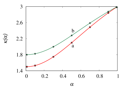
Figure 5: Kurtosis $\kappa(\alpha)$ vs $\alpha$. Symbols are the results of stochastic simulations, lines represent the analytical expressions eqs. (70), (75). Line (a) and ($\circ$): 2d case, line (b) and ($\square$): 3d case.

Figure 5 depicts the simulation results for the kurtosis compared with the analytical predictions eqs. (70), (75). These results refer to an ensemble of $10^{9}$ realizations of the process.

The density functions for a generic entry of the velocity field (say $v_{1}$ in the 2d case and $v_{3}$ in the 3d case) are depicted is figures 6 and 7 for the 2d and the 3d case, respectively. The velocities appearing in these figures are normalized to unit variance.

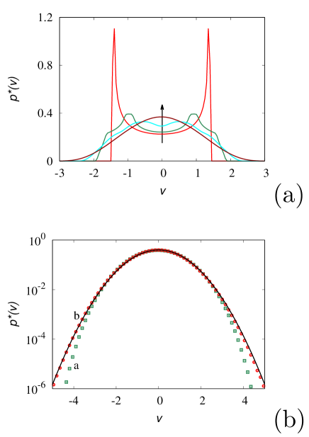
Figure 6: Equilibrium velocity distribution $p^{*}(v)$ of a generic Cartesian entry of ${\bf v}$ in the 2d case. Panel (a) refers to $\alpha=0.1,\,0.3,\,0.5,\,0.7$. The arrow indicates increasing values of $\alpha$. Panel (b) refers to high values of $\alpha$: symbols ($\square$) correspond to stochastic simulations at $\alpha=0.9$, symbols ($\circ$) at $\alpha=0.99$. The solid line represents the normal distribution $p_{n}(v)$.

As expected from the analysis of the kurtosis, for low values of $\alpha$, these distributions deviate significantly from the normal distribution $p_{n}(v)$,

$$p_{n}(v)=\frac{1}{\sqrt{2\,\pi}}\,e^{-v^{2}/2}$$ (77)

In the limit for $\alpha\rightarrow 1$, $p^{*}(v)$ approaches $p_{n}(v)$ as expected. Already at $\alpha=0.99$ the resulting normalized velocity density is indistinguishable from the normal distribution.

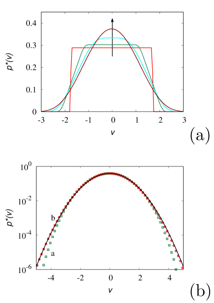
Figure 7: Equilibrium velocity distribution $p^{*}(v)$ of a generic Cartesian entry of ${\bf v}$ in the 3d case. Panel (a) refers to $\alpha=0.1,\,0.3,\,0.5,\,0.7$. The arrow indicates increasing values of $\alpha$. Panel (b) refers to high values of $\alpha$: symbols ($\square$) correspond to stochastic simulations at $\alpha=0.9$, symbols ($\circ$) at $\alpha=0.99$. The solid line represents the normal distribution $p_{n}(v)$.

The equilibrium distributions $f^{*}(|{\bf v}|)$ for the modulus of the normalized velocity $|{\bf v}|$ are depicted in figure 8 for the sake of completeness, although they do not add any further physical insight to the above analysis of velocity statistics.

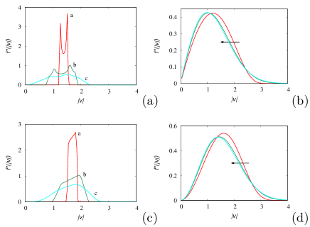
Figure 8: Equilibrium distributions $f^{*}(|{\bf v}|)$ of the modulus $|{\bf v}|$ obtained from stochastic simulations. Panels (a) and (b): 2d case, panels (c) and (d): 3d case. Lines (a) refer to $\alpha=0.1$, lines (b) to $\alpha=0.3$, lines (c) to $\alpha=0.5$. The arrows in panels (b) and (d) indicate increasing values of $\alpha=0.7,\,0.9,\,0.99$.

As regards the two asymptotic distributions obtained in the limit for $\alpha\rightarrow 1$ and $\alpha\rightarrow 0$, their mathematical justification is rather straightforward, but their physical interpretation is rather interesting.

As discussed above, the Gaussian profile is recovered in the limit for $\alpha\rightarrow 1$. In the present case, this corresponds to the situation in which the velocity dynamics possesses the strongest memory of its past history. The latter interpretation follows also from the exponential decay of the velocity autocorrelation function that, for $\alpha\rightarrow 1$, is characterized by an exponent $\eta_{r}/m\rightarrow 0$. In this sense the fluctuation-dissipation relation can be viewed as a dissipation-memory condition for particle-photon interactions (momentum exchange).

In the particle-photon dynamics described by eq. (36) the above mentioned memory effects (that should not be confused with the lack of Markovianity, as the process is strictly Markovian, and its transition mechanism has no memory) determine the occurrence of a normal distribution for the velocity entries. This phenomenon can be easily interpreted by considering the simplest linear relaxation dynamics for an observable $y(t)$,

$$\frac{dy(t)}{dt}=-\ell\,y(t)-f(t)$$ (78)

where $f(t)$ is a stochastic impulsive forcing and $\ell>0$ the relaxation rate, the solution of which, neglecting the decaying initial condition, is expressed by the convolutional integral

$$y(t)=\int_{0}^{t}e^{-\ell(t-\tau)}\,f(\tau)\,d\tau$$ (79)

Assuming $f(t)=\sum_{i=1}^{\infty}f_{i}\,\delta(t-t_{i}^{*})$, where $t_{i}^{*}<t_{i+1}^{*}$m and $f_{i}$ generic random variables, we have in the limit for $\ell\rightarrow 0$ that

$$y(t)=\sum_{i=1}^{n(t)}f_{i}$$ (80)

where $n(t)$ is the integer $n(t)=\sum_{i=1}^{\infty}\int_{0}^{t}\delta(\tau-t_{i}^{*})\,d\tau$.

Eq. (79) clearly indicates that the only physical way for the velocity dynamics could perform a summation of the random photon momentum kicks, corresponding to the classical setting of the Central Limit Theorem, is to possess an infinite memory of its past history, corresponding to $\ell\rightarrow 0$. In this case, the velocity dynamics corresponds to the summation of the independent random kicks induced by the photon bath.

It is also interesting to consider the other limit, namely $\alpha\rightarrow 0$, corresponding to the complete absence of memory in velocity dynamics, as eq. (44) reduces in this limit to

$${\bf v}_{n+1}=\beta\,{\bf r}_{n+1}$$ (81)

and consequently, the velocity statistics is simply a rescaled sampling of the statistics of photon momenta. Consider the 2d case, and let $v$ a velocity entry, say $v_{1}$, for which in the limit for $\alpha\rightarrow 0$ we have (upon normalization)

$$v=\sqrt{2}\,\cos\phi$$ (82)

$\phi$ being uniformly distributed in $[0,2\pi)$. The equilibrium distribution function for $v$ is thus given by

$$F^{*}(v) = \frac{1}{2\,\pi}\int_{\{\sqrt{2}\,\cos\phi<v\}}\,d\phi=\frac{1}{\pi}\int_{\arccos y/\sqrt{2}}^{\pi}d\phi$$ (83)

$$= =1-\frac{1}{\pi}\arccos\left(\frac{v}{\sqrt{2}}\right)$$

in the interval $v\in(-\sqrt{2},\sqrt{2})$, while $F^{*}(v)=0$ for $v<-\sqrt{2}$ and $F^{*}(v)=1$ for $v>\sqrt{2}$. Differentiating $F_{v}^{*}(v)$ with respect to $v$, the density function $p^{*}(v)$ follows

$$p^{*}(v)=\frac{1}{\sqrt{2}\,\pi}\,\frac{1}{\sqrt{1-v^{2}/2}}\,,\qquad v\in(-\sqrt{2},\sqrt{2})$$ (84)

and zero otherwise. Figure 9 panel (a) compares the results of stochastic simulations of the velocity dynamics via eq. (44) at low $\alpha$-values, and the analytical expression for the limit velocity density function eq. (84) in the 2d case.

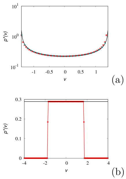
Figure 9: Equilibrium velocity distribution $p^{*}(v)$ at low $\alpha$-values. Panel (a) refers to the 2d case. Symbols represent the results of stochastic simulations at $\alpha=0.01$ ($\square$), and $\alpha=10^{-6}$ ($\circ$). The solid line is the analytical expression eq. (84). Panel (b) refers to the 3d case. Symbols represent the results of stochastic simulations at $\alpha=0.01$. the horizontal line is the analytical value $p^{*}(v)=1/2\sqrt{3}$.

Analogously, in the 3d case, by considering $v=v_{3}=\sqrt{3}\,\cos\theta$, $\theta\in[0,\pi)$, we have

$$F^{*}(v)=\frac{1}{2}\,\int_{\arccos(v/\sqrt{3})}^{\pi}\,\sin\theta\,d\theta=\frac{1}{2}\,\left(1+\frac{v}{\sqrt{3}}\right)$$ (85)

in $v\in(-\sqrt{3},\sqrt{3})$. Consequently, the density function $p^{*}(v)$ is piecewise constant in the limit for $\alpha\rightarrow 0$,

$$p^{*}(v)=\left\{\begin{array}[]{lll}\frac{1}{2\,\sqrt{3}}&&v\in(-\sqrt{3},\sqrt{3})\\ 0&&\mbox{otherwise}\end{array}\right.$$ (86)

as depicted in figure 9 panel (b).

This result is interesting from another point of view. The case $\alpha\rightarrow 0$, corresponds physically to $\gamma\rightarrow\infty$, i.e. to the low-temperature limit. In these conditions, the statistics of particle velocity corresponds to the pure sampling of the randomness in the orientation of the incoming photons. Due to isotropy, these orientations are distributed uniformly on the surface of the unit sphere. As can be observed from figure 9 and from the calculations in the main text, the shape of the equilibrium distributions $p^{*}(v)$ strongly depends qualitatively on the dimension of the physical space in which photons travel. Therefore, it is conceptually possible the experimental determination of the dimension $d$, $d=2,3,\dots$, of the physical space from measurements of $p^{*}(v)$.

VII Concluding remarks

This article has focused on radiative processes and their thermalization properties in molecular systems (gases), neglecting the influence of particle-particle collisions. This restriction is aimed at isolating the role of emission/absorption processes for understanding their peculiar features. The interplay between radiative processes and elastic collisions will be addressed in a forthcoming work. Under these conditions, the equation for the temporal evolution of particle momentum can be expressed in the form of a nonlinear impulsive differential equation, driven by the distributional derivative of a Poisson counting process. This formulation, that accounts for the Einsteinian representation of radiative processes, introduces the concept of a radiative mass $\eta$, describing statistically the dissipative recoil effect associated with a radiative transition between two energy levels. At high temperatures, the radiative mass is smaller than the inertial mass, while it diverges for $T\rightarrow 0$. From this formulation, a radiative fluctuation-dissipation theorem can be derived, associated with the exponential decay of the velocity autocorrelation function.

The velocity distribution function has been thoroughly analyzed. In the limit of small radiative friction, the velocity distribution converges to the Maxwellian (Gaussian) profile, while in the limit of high radiative dissipation it converges to eq. (83) controlled by the random and uniform distribution of the incoming/emitted photons. Deviations from Gaussianity are not surprinsing, as the momentum equation (36), bears some similarity with the approach followed in athermal1 for the statistical mechanical properties of athermal system. For the sake of completeness, it should be observed that, while the values of $\langle v_{i}^{2}\rangle$ are not affected by elastic particle-particle collisions, the latter modify significantly the shape of the velocity distribution function.

Appendix - Nonlinear impulsive differential equations

The analysis of differential equations of the form (36),(37) in which the impulsive forcing is modulated by a function of the unknown variable (situation that can be referred to as a nonlinear impulsive differential equation, in analogy with the definition of nonlinear Langevin equations) poses mathematical problems similar to those encountered for the nonlinear Langevin equations (driven by a Wiener forcing), associated with the Ito-Stratonovich dilemma. The mathematical problems arise because the function ${\bf v}(t)$ is discontinuous at $t=t^{*}$ and, therefore, a rule should be specified to intepret this equation. In most of the literature imp1 ; imp2 ; imp3 a mid-point rule as been adopted. Let ${\bf v}={\bf v}(t^{*}_{-})$ and ${\bf v}^{\prime}={\bf v}(t_{+}^{*})$, where $t^{*}_{\pm}=\lim_{\varepsilon\rightarrow 0}{\bf v}(t^{*}\pm\varepsilon)$, $\varepsilon>0$, and integrate eq. (37) in the interval $[t^{*}-\varepsilon,t^{*}+\varepsilon]$ taking the limit for $\varepsilon\rightarrow 0$,

$$m\,({\bf v}^{\prime}-{\bf v})=\int_{t^{*}_{-}}^{t^{*}_{+}}(-\eta\,{\bf v}(t)+{\bf b})\,\delta(t-t^{*})\,dt$$ (87)

the mid-point rule assumes that for the integral containing ${\bf v}$

$$\int_{t^{*}_{-}}^{t^{*}_{+}}{\bf v}(t)\,\delta(t-t^{*})\,dt=\frac{{\bf v}^{\prime}+{\bf v}}{2}$$ (88)

so that eq. (87) becomes

$$m\,({\bf v}^{\prime}-{\bf v})=-\eta\,\left(\frac{{\bf v}^{\prime}+{\bf v}}{2}\right)+{\bf b}$$ (89)

This approach has been critically confuted in impulsive_critic on the basis of simple principles of calculus. In point of fact, expressing eq. (37) conponentwise,

$$m\,\frac{dv_{i}}{\eta\,v_{i}-b_{i}}=-\delta(t-t^{*})\,dt$$ (90)

$i=1,2,3$, integrating over $(t^{*}_{-},t_{+}^{*})$,

$$\frac{m}{\eta}\int_{t_{-}^{*}}^{t_{+}^{*}}\frac{dv_{i}}{v_{i}-b_{i}/\eta}=-\int_{t_{-}^{*}}^{t_{+}^{*}}\delta(t-t^{*})\,dt$$ (91)

one finally obtains

$$\frac{m}{\eta}\,\log\left(\frac{v_{i}^{\prime}-b_{i}/\eta}{v_{i}-b_{i}/\eta}\right)=-1$$ (92)

leading to eq. (38). In the limit for $\eta/m\ll 1$, the mid-point rule is recovered.

References

- (1) D. Bohm, Quantum Theory, (Dover Publ., New York,1989).
- (2) C. Cohen-Tannoudji, J. Dupont-Roc and G. Grynberg, Atom-Photon Interactions, (Wiley-VCH, Weinhheim, 2004).
- (3) T. L. Hill, Introduction to Statistical Thermodynamics, (Dover Publ., New York, 1986).
- (4) R. H. Fowler, Statistical Mechanics, (Cambridge Univ. Press, Cambridge, 1929).
- (5) A. Einstein, and O. Stern, Ann. Phys. (Berlin) 40, 1913, 551.
- (6) P. Debye, Ann. Phys. (Berlin) 39, 1912, 784.
- (7) A. Ashkin and J. M. Dziedzic, Science 235, 1987, 1517
- (8) G. Bolognesi, M. S. Friddin, A. Salehi-Reyhani, N. E. Barlow, N. J. Brooks, O. Ces and Y Elani, Nature commu. 9, 2018, 1.
- (9) Y. Yang, Y. Ren, M. Chen, Y. Arita, and C. Rosales-Guzmán, Adv. Photonics 2021, 3 034001.
- (10) A. Ashkin, Phys. Rev. Lett. 24, 1970, 156.
- (11) S. Sternholm, Rev. Mod. Phys. 58, 1986, 699.
- (12) W. D. Phillips, Rev. Mod. Phys. 70, 1998, 721.
- (13) H. J. Metcalf and P. van der Straten, Laser Cooling and Trapping, (Springer, New York, 1999).
- (14) A. Einstein, Phys. Zeit. 18, 1917, 121.
- (15) C. Pezzotti and M. Giona, ”Chemical kinetics and stochastic differential equations”, in preparation.
- (16) A. Lami and N. K. Rahman, Phys. Rew. A 32, 1985, 901.
- (17) P. W. Milonni, The Quantum Vacuum. An Introduction to Quantum Electrodynamics, (Academic Press, San Diego, 1994).
- (18) D. Dalvit, P. Milonni, D. Roberts and F. da Rosa (Eds.), Casimir Physics, (Springer-Verlag, Brlin, 2011).
- (19) W. M. R. Simpson and U. Leonhardt, Forces of Quantum Vacuum, (World Scientific, New Jersey, 2015).
- (20) S. G. Pandit and S. G. Deo, Differential Systems Involving Impulses, (Springer-Verlag, Berlin, 1982).
- (21) A. J. Catlá, D. G. Schaeffer, T. P. Witelski, E. E. Monson and A. L. Lin, SIAM Review 50, 2008, 553.
- (22) S. Balasuriya, Nonlinearity 29, 2016, 3897.
- (23) D. Griffiths and S. Walborn, Am. J. Phys. 67, 1999, 446.
- (24) N. Van Kampen, J. Stat. Phys. 24, 1981, 175.
- (25) P. E. Kloeden and E. Platen, Numerical solution of stochatsic differential equations, (Springer, Berlin, 1992).
- (26) K. Kanazawa, T. G. Sano, T. Sagawa and H. Hayakawa, Phys. Rev. Lett. 114, 2015, 090601.