Strong SDP based bounds on the cutwidth of a graph

Abstract

Given a linear ordering of the vertices of a graph, the cutwidth of a vertex $v$ with respect to this ordering is the number of edges from any vertex before $v$ (including $v$) to any vertex after $v$ in this ordering. The cutwidth of an ordering is the maximum cutwidth of any vertex with respect to this ordering. We are interested in finding the cutwidth of a graph, that is, the minimum cutwidth over all orderings, which is an NP-hard problem. In order to approximate the cutwidth of a given graph, we present a semidefinite relaxation. We identify several classes of valid inequalities and equalities that we use to strengthen the semidefinite relaxation. These classes are on the one hand the well-known 3-dicycle equations and the triangle inequalities and on the other hand we obtain inequalities from the squared linear ordering polytope and via lifting the linear ordering polytope. The solution of the semidefinite program serves to obtain a lower bound and also to construct a feasible solution and thereby having an upper bound on the cutwidth.

In order to evaluate the quality of our bounds, we perform numerical experiments on graphs of different sizes and densities. It turns out that we produce high quality bounds for graphs of medium size independent of their density in reasonable time. Compared to that, obtaining bounds for dense instances of the same quality is out of reach for solvers using integer linear programming techniques.

1 Introduction

Several graph parameters are determined by finding an arrangement of the vertices of a graph on a straight line having a certain objective in mind. Depending on the objective, these parameters are, for instance, the treewidth, the pathwidth, the bandwidth or the cutwidth of a graph. Computing these graph parameters is necessary for several applications, e.g., when a certain layout has to be found (VLSI design, see Raspaud et al. (1995)), in automatic graph drawing, see Díaz et al. (2002), or in many versions of network problems arising in energy or logistics. All these applications ask for algorithms to practically compute these parameters. However, this leads to NP-hard optimization problems and therefore algorithms for approximating these parameters in terms of lower and upper bounds are required. The parameter that is of our interest in this work is the cutwidth of a graph.

Definitions.

The minimum cutwidth problem (MCP) can be defined as follows. We consider an undirected graph $G=(V,E)$ with vertex set $V$ and edge set $E$ and assume without loss of generality that the set of vertices $V$ is $V=\{1,\dots,n\}$. Furthermore, the set of all permutations of $\{1,\dots,n\}$ is denoted by $\Pi_{n}$. In any permutation $\pi\in\Pi_{n}$ of the vertices of $G$, the position of a vertex $v\in V$ in $\pi$ is given by $\pi(v)$. Note that any linear ordering of the vertices $V$ of $G$ can be represented by a permutation $\pi\in\Pi_{n}$.

The cutwidth $CW_{\pi}(v)$ of a vertex $v$ with respect to the permutation $\pi$ is the number of edges $\{u,w\}\in E$ such that $\pi(u)\leq\pi(v)<\pi(w)$ holds, i.e., the cutwidth of $v$ in $\pi$ is the number of edges from any vertex before $v$ (including $v$) to any vertex after $v$ (not including $v$) in a linear ordering of the vertices according to the permutation $\pi$. Furthermore, the cutwidth $CW_{\pi}(G)$ of a graph $G$ with respect to $\pi$ is the maximum cutwidth of any vertex with respect to the permutation $\pi$, so

$$CW_{\pi}(G)=\max_{v\in V}CW_{\pi}(v)$$

holds. Finally, the cutwidth $CW(G)$ of a graph $G$ is the minimum cutwidth of $G$ with respect to $\pi$ over all possible permutations $\pi$, i.e.,

$$CW(G)=\min_{\pi\in\Pi_{n}}CW_{\pi}(G).$$

An obvious lower bound on the cutwidth is given by

$$CW(G)\geq\lfloor\frac{\Delta(G)+1}{2}\rfloor,$$

where $\Delta(G)$ is the maximum degree of any vertex in $V$. Indeed, let us denote by $v_{\max}$ a vertex of G with degree $\Delta(G)$. Then, for every linear ordering $\pi$, every vertex in the neighborhood of $v_{\max}$ is counted either in $CW_{\pi}(v_{\max})$ or in $CW_{\pi}(u_{\max})$, where $u_{\max}$ is the vertex directly preceding $v_{\max}$ in $\pi$. It follows that either $CW_{\pi}(v_{\max})$ or $CW_{\pi}(u_{\max})$ has to be greater or equal to ${\frac{\Delta(G)}{2}}$, and due to the integrality of $CW(G)$ we obtain the lower bound $\lfloor\frac{\Delta(G)+1}{2}\rfloor$.

Among connected graphs with $n$ vertices, the graphs with the smallest cutwidth are the paths, which have a cutwidth of 1. The graphs with the largest cutwidth are the complete graphs $K_{n}$, with $CW(K_{n})=\lfloor\frac{n²}{4}\rfloor$.

Related literature.

The MCP has been investigated in several aspects and in several contexts. Inspired from results in the topology of manifolds, Kloeckner (2009) explores lower bounds depending on the sparsity and the degeneracy of the underlying graph. Next to theoretical properties of the cutwidth, connections between the cutwidth of a graph $G$ with its treewidth $TW(G)$ and its pathwidth $PW(G)$ have been explored by several authors. It is known that $CW(G)\leq\Delta(G)PW(G)$ from Chung and Seymour (1989), $CW(G)\geq TW(G)$ from Bodlaender (1986), and $CW(G)=\mathcal{O}((\log n)\Delta(G)TW(G))$ from Korach and Solel (1993). It follows that if $TW(G)$ and $\Delta(G)$ are bounded by constants, $CW(G)=\mathcal{O}(\log n)$. Furthermore, if $(X,T)$ is a tree decomposition of $G$ with treewidth $k$, then $CW(G)\leq(k+1)\Delta(G)CW(T)$.

As for computing the cutwidth, there exist polynomial time algorithms for certain graph classes, see e.g. Heggernes et al. (2011, 2012); Yannakakis (1985). Giannopoulou et al. (2019) design a fixed-parameter algorithm for computing the cutwidth that runs in time $2^{\mathcal{O}(k^{2}\log{}k)}n$, where $k$ is the cutwidth. In a more general setting, Bodlaender et al. (2012) discuss exponential time algorithms for vertex ordering problems, including the MCP. A relation of computing the cutwidth and the pathwidth via the so-called locality number, a structural parameter for strings, has been investigated by Casel et al. (2019).

Another way to solve the MCP is to model the optimization problem as a mixed-integer linear program (MILP). This has been considered by Luttamaguzi et al. (2005) and by López-Locés et al. (2014). Moreover, in the PhD thesis of Coudert (2016a) MILP formulations for linear ordering problems, among them the cutwidth, pathwidth and bandwidth problem, are given. Therein, different formulations for these problems are introduced and compared to each other. However, all these algorithms can only deal with sparse instances of small size. Indeed, by Coudert (2016a) results are given for (very) sparse graphs only with $|V|\in\{16,\dots,24\}$.

Martí et al. (2013) introduce a branch-and-bound algorithm using lower bounds on the cutwidth of partial solutions and a greedy randomized adaptive search procedure (GRASP) to compute upper bounds. Applying the metaheuristic adaptive large neighborhood search for obtaining orderings with a small cutwidth has been introduced by Santos and de Carvalho (2021).

A further line of research is to apply semidefinite programming (SDP) to optimization problems that deal with orderings of the vertices, see e.g. Buchheim et al. (2010); Hungerländer and Rendl (2013). In particular, SDP based methods proved to be very successful when applied to the single row facility layout problem, see Fischer et al. (2019); Schwiddessen (2022), which falls into this category as its goal is to order facilities on a straight line in the best way according to some objective function. SDP based bounds for the bandwidth problem are introduced in Rendl et al. (2021). To the best of our knowledge there have been no attempts so far in using semidefinite programming to tackle the MCP.

Contribution and outline.

In this paper we present a novel relaxation of the MCP that uses semidefinite programming. We introduce several valid inequalities that we include in the SDP in a cutting-plane fashion to strengthen the lower bound on the cutwidth. Moreover, we introduce a heuristic that uses the optimizer of the SDP to obtain feasible solutions and thereby providing an upper bound on the cutwidth. Our computational experiments confirm that we can obtain tight bounds in reasonable time and that the run time of our algorithms are not sensitive concerning the density of the graph.

The rest of this paper is structured as follows. In Section 2 we introduce a basic SDP relaxation for the MCP and provide several linear constraints that can be used to strengthen the basic SDP relaxation. We describe in detail the algorithm for computing the lower bounds arising from the SDP as well as a heuristic to obtain upper bounds in Section 3. Computational results of our new algorithms are given in Section 4, and Section 5 concludes.

2 New bounds for the minimum cutwidth problem

The aim of this section is to introduce a new SDP relaxation for the MCP and to present ways to strengthen this relaxation.

2.1 Our new basic SDP relaxation

We follow the approach of Buchheim et al. (2010) for the quadratic linear ordering problem in order to derive an SDP formulation of the MCP. This is a promising endeavor, as the feasible region of both the quadratic linear ordering problem and the MCP consist of permutations.

Towards this end, let $A=(a_{ij})_{1\leq i,j\leq n}$ be the adjacency matrix of the graph $G$, i.e., $a_{ij}=1$ if and only if the edge $\{i,j\}$ is in the set of edges $E$ of the graph $G$. To represent a permutation $\pi$, Buchheim et al. (2010) introduce a binary variable $\chi^{\pi}_{ij}$ for any $1\leq i<j\leq n$ that indicates whether $\pi(i)<\pi(j)$ holds, so in total they have a vector $\chi^{\pi}$ consisting of $\binom{n}{2}$ binary variables. They define the linear ordering polytope $LO(n)$ as the convex hull of all vectors $\chi^{\pi}$, formally

$$LO(n)=\operatorname{conv}\{\chi^{\pi}\colon\pi\in\Pi_{n}\},$$

which is a subset of $\mathbb{R}^{\binom{n}{2}}$. As a consequence, the elements of the set $LO(n)\cap\{0,1\}^{\binom{n}{2}}$ are exactly all vectors representing permutations of $\{1,\dots,n\}$.

Let $x=(x_{ij})_{1\leq i<j\leq n}$ be a vector in $LO(n)\cap\{0,1\}^{\binom{n}{2}}$ representing a permutation $\pi\in\Pi_{n}$. By definition, the binary variable $x_{ij}$ is equal to $1$ if and only if $i$ is before $j$ in $\pi$. Then, it can be checked that for any vertex $v$ of $G$,

$$CW_{\pi}(v)= \sum_{\begin{subarray}{c}u\in V\\ u<v\end{subarray}}\sum_{\begin{subarray}{c}w\in V\\ w>v\end{subarray}}a_{uw}x_{uv}x_{vw}+\sum_{\begin{subarray}{c}u\in V\\ u>v\end{subarray}}\sum_{\begin{subarray}{c}w\in V\\ w>v\\ w\neq u\end{subarray}}a_{uw}(1-x_{vu})x_{vw}+\sum_{\begin{subarray}{c}u\in V\\ u<v\end{subarray}}\sum_{\begin{subarray}{c}w\in V\\ w<v\\ w\neq u\end{subarray}}a_{uw}x_{uv}(1-x_{wv})$$

$$+\sum_{\begin{subarray}{c}u\in V\\ u>v\end{subarray}}\sum_{\begin{subarray}{c}w\in V\\ w<v\end{subarray}}a_{uw}(1-x_{vu})(1-x_{wv})+\sum_{\begin{subarray}{c}w\in V\\ w>v\end{subarray}}a_{vw}x_{vw}+\sum_{\begin{subarray}{c}w\in V\\ w<v\end{subarray}}a_{vw}(1-x_{wv})$$ (1)

holds. The first four terms of this expression count the number of edges from any vertex before $v$ to any vertex after $v$ in the permutation, both not including $v$. These four terms are necessary, as only one of the variables $x_{uv}$ (if $u<v$) and $x_{vu}$ (if $u>v$), and one of the variables $x_{wv}$ (if $w<v$) and $x_{vw}$ (if $w>v$) exist. The last two terms of (2.1) count the edges from $v$ to any vertex after $v$.

By expanding (2.1), grouping the constant, linear and quadratic terms together, and by combining three times two sums as one, we can rewrite (2.1) as

$$CW_{\pi}(v) =\sum_{\begin{subarray}{c}w\in V\\ w<v\end{subarray}}\sum_{\begin{subarray}{c}u\in V\\ u\geq v\end{subarray}}a_{uw}+\sum_{\begin{subarray}{c}w\in V\\ w>v\end{subarray}}\sum_{\begin{subarray}{c}u\in V\\ u\geq v\\ {u\neq w}\end{subarray}}a_{uw}x_{vw}+\sum_{\begin{subarray}{c}u\in V\\ u<v\end{subarray}}\sum_{\begin{subarray}{c}w\in V\\ w<v\\ {w\neq u}\end{subarray}}a_{uw}x_{uv}$$ (2)

$$\phantom{\geq}-\sum_{\begin{subarray}{c}u\in V\\ u>v\end{subarray}}\sum_{\begin{subarray}{c}w\in V\\ w<v\end{subarray}}a_{uw}(x_{vu}+x_{wv})-\sum_{\begin{subarray}{c}w\in V\\ w<v\end{subarray}}a_{vw}x_{wv}+2\sum_{\begin{subarray}{c}u\in V\\ u<v\end{subarray}}\sum_{\begin{subarray}{c}w\in V\\ w>v\end{subarray}}a_{uw}x_{uv}x_{vw}$$

$$\phantom{\geq}-\sum_{\begin{subarray}{c}u\in V\\ u>v\end{subarray}}\sum_{\begin{subarray}{c}w\in V\\ w>v\\ {w\neq u}\end{subarray}}a_{uw}x_{vu}x_{vw}-\sum_{\begin{subarray}{c}u\in V\\ u<v\end{subarray}}\sum_{\begin{subarray}{c}w\in V\\ w<v\\ {w\neq u}\end{subarray}}a_{uw}x_{uv}x_{wv},$$

and as a result, the MCP can be written as

$$\min \leavevmode\nobreak\ \alpha$$ (3a)

$$\operatorname{s.t.}\leavevmode\nobreak\ \alpha \geq\sum_{\begin{subarray}{c}w\in V\\ w<v\end{subarray}}\sum_{\begin{subarray}{c}u\in V\\ u\geq v\end{subarray}}a_{uw}+\sum_{\begin{subarray}{c}w\in V\\ w>v\end{subarray}}\sum_{\begin{subarray}{c}u\in V\\ u\geq v\\ {u\neq w}\end{subarray}}a_{uw}x_{vw}+\sum_{\begin{subarray}{c}u\in V\\ u<v\end{subarray}}\sum_{\begin{subarray}{c}w\in V\\ w<v\\ {w\neq u}\end{subarray}}a_{uw}x_{uv}$$ (3b)

$$\phantom{\geq}-\sum_{\begin{subarray}{c}u\in V\\ u>v\end{subarray}}\sum_{\begin{subarray}{c}w\in V\\ w<v\end{subarray}}a_{uw}(x_{vu}+x_{wv})-\sum_{\begin{subarray}{c}w\in V\\ w<v\end{subarray}}a_{vw}x_{wv}+2\sum_{\begin{subarray}{c}u\in V\\ u<v\end{subarray}}\sum_{\begin{subarray}{c}w\in V\\ w>v\end{subarray}}a_{uw}x_{uv}x_{vw}\quad$$

$$\phantom{\geq}-\sum_{\begin{subarray}{c}u\in V\\ u>v\end{subarray}}\sum_{\begin{subarray}{c}w\in V\\ w>v\\ {w\neq u}\end{subarray}}a_{uw}x_{vu}x_{vw}-\sum_{\begin{subarray}{c}u\in V\\ u<v\end{subarray}}\sum_{\begin{subarray}{c}w\in V\\ w<v\\ {w\neq u}\end{subarray}}a_{uw}x_{uv}x_{wv} \forall v\in V$$

$$x \in LO(n)\cap\{0,1\}^{\binom{n}{2}}.$$ (3c)

This is an integer program with a linear objective function and quadratic constraints, which is perfectly suited for deriving an SDP relaxation. To do so, we introduce the matrix variable $X=(X_{ij,k\ell})_{\begin{subarray}{c}1\leq i<j\leq n\\ 1\leq k<\ell\leq n\end{subarray}}$. In particular, $X_{ij,k\ell}$ represents the product $x_{ij}x_{k\ell}$. Then the following SDP is a relaxation of the MCP.

$$\min \alpha$$ (4a)

$$\operatorname{s.t.}\leavevmode\nobreak\ \alpha \geq\sum_{\begin{subarray}{c}w\in V\\ w<v\end{subarray}}\sum_{\begin{subarray}{c}u\in V\\ u\geq v\end{subarray}}a_{uw}+\sum_{\begin{subarray}{c}w\in V\\ w>v\end{subarray}}\sum_{\begin{subarray}{c}u\in V\\ u\geq v\\ {u\neq w}\end{subarray}}a_{uw}x_{vw}+\sum_{\begin{subarray}{c}u\in V\\ u<v\end{subarray}}\sum_{\begin{subarray}{c}w\in V\\ w<v\\ {w\neq u}\end{subarray}}a_{uw}x_{uv}$$ (4b)

$$\phantom{\geq}-\sum_{\begin{subarray}{c}u\in V\\ u>v\end{subarray}}\sum_{\begin{subarray}{c}w\in V\\ w<v\end{subarray}}a_{uw}(x_{vu}+x_{wv})-\sum_{\begin{subarray}{c}w\in V\\ w<v\end{subarray}}a_{vw}x_{wv}+2\sum_{\begin{subarray}{c}u\in V\\ u<v\end{subarray}}\sum_{\begin{subarray}{c}w\in V\\ w>v\end{subarray}}a_{uw}X_{uv,vw}\quad$$

$$\phantom{\geq}-\sum_{\begin{subarray}{c}u\in V\\ u>v\end{subarray}}\sum_{\begin{subarray}{c}w\in V\\ w>v\\ {w\neq u}\end{subarray}}a_{uw}X_{vu,vw}-\sum_{\begin{subarray}{c}u\in V\\ u<v\end{subarray}}\sum_{\begin{subarray}{c}w\in V\\ w<v\\ {w\neq u}\end{subarray}}a_{uw}X_{uv,wv}\qquad \forall v\in V$$

$$x =\operatorname{diag}(X)$$ (4c)

$$\bar{X} =\begin{pmatrix}1&x^{\top}\\ x&X\end{pmatrix}$$ (4d)

$$\bar{X} \succeq 0.$$ (4e)

Note that $x=(x_{ij})_{1\leq i<j\leq n}$ is a vector of dimension $\binom{n}{2}$ and $\bar{X}$ is a square matrix with $(\binom{n}{2}+1)$ columns and rows. Thus, the SDP (4) has a matrix variable of dimension $(\binom{n}{2}+1)$ and $n+\binom{n}{2}+1$ constraints. The $n$ constraints (4b) make sure that $\alpha$ is at least the cutwidth of each vertex. The $\binom{n}{2}+1$ constraints (4c) together with the constraints (4d) and (4e) represent the relaxation of $X-xx^{\top}=0$ to $X-xx^{\top}\succeq 0$ and taking the Schur complement. Due to the fact that $x$ is binary, $X-xx^{\top}=0$ also implies that (4c) has to hold.

Furthermore, note that adding the non-convex constraint $\operatorname{rank}(\bar{X})=1$ to the SDP relaxation (4), the optimal objective function value becomes $CW(G)$. This is also the case if we add integer conditions for $X$.

2.2 Strengthening the SDP relaxation

Next, we investigate several options to improve the SDP relaxation (4) of the MCP.

2.2.1 3-dicycle equations

In the basic SDP relaxation (4), no specific information about the fact that $x$ should represent a permutation is used. One possible way to include such information is to model the transitivity by so-called 3-dicycle equations, as it is done by Buchheim et al. (2010). These 3-dicycle equations make sure that if $i$ is before $j$ and $j$ is before $k$, then $i$ must be before $k$. For a vector $x=(x_{ij})_{1\leq i<j\leq n}$, they can be written as

$$x_{ik}-x_{ij}x_{ik}-x_{ik}x_{jk}+x_{ij}x_{jk}=0 \quad\forall i<j<k,$$ (5)

so we can include

$$x_{ik}-X_{ij,ik}-X_{ik,jk}+X_{ij,jk}=0 \quad\forall i<j<k$$ (6)

as additional constraints into our SDP relaxation (4) of the MCP. If we add all possible constraints of the form (6), we include $\binom{n}{3}$ equality constraints.

Observe, that Buchheim et al. (2010) show that if the variables are binary, the expression on the left hand-side of (5) is always non-negative. So in this case, one needs to consider only the inequality $\leq 0$. However, this does not hold anymore for our SDP relaxation, as the variables are not necessarily binary.

2.2.2 Triangle inequalities

Another way to strengthen the SDP relaxation (4) is adding the triangle inequalities

$$0 \leq X_{ij,k\ell} \forall i<j,k<\ell$$ (7a)

$$X_{ij,k\ell} \leq X_{ij,ij} \forall i<j,k<\ell$$ (7b)

$$X_{ij,ij}+X_{k\ell,k\ell} \leq 1+X_{ij,k\ell} \forall i<j,k<\ell$$ (7c)

$$X_{ij,k\ell}+X_{uv,k\ell} \leq X_{k\ell,k\ell}+X_{ij,uv} \forall i<j,k<\ell,u<v$$ (7d)

$$X_{ij,ij}+X_{k\ell,k\ell}+X_{uv,uv} \leq 1+X_{ij,k\ell}+X_{ij,uv}+X_{k\ell,uv} \forall i<j,k<\ell,u<v.$$ (7e)

The inequalities (7a) and (7b) were introduced by Lovász and Schrijver (1991) and the constraints (7c), (7d) and (7e) originate from Gruber and Rendl (2003). As a consequence, (7a), (7b) and (7c) each yield $\binom{n}{2}^{2}$ potential new constraints. Both (7d) and (7e) offer the option of including $\binom{n}{2}^{3}$ inequalities.

It can be checked easily that all the inequalities of (7) are satisfied for each matrix $X=xx^{\top}$ for any $x\in LO(n)\cap\{0,1\}^{\binom{n}{2}}$, so for any vector $x$ that represents a permutation. Thus, the inequalities (7) are valid inequalities for the SDP relaxation (4) for the MCP. Next, we give an alternative reasoning that the inequalities (7) are satisfied.

2.2.3 Inequalities obtained from the squared linear ordering polytope

Adams et al. (2015) introduced so-called exact subgraph constraints (ESC), which were later computationally exploited for the stable set problem, the Max-Cut problem and the coloring problem by Gaar and Rendl (2019, 2020).

For the stable set problem the ESCs are defined in the following way. Let $G=(V,E)$ be a graph with vertex set $V=\{1,2,\dots,n\}$. The squared stable set polytope $STAB^{2}(G)$ of $G$ is defined as

$$STAB^{2}(G)=\operatorname{conv}\left\{ss^{T}:s\in\{0,1\}^{n},s_{i}s_{j}=0\quad\forall\{i,j\}\in E\right\},$$

and the ESCs for the stable set problem (ESCSS) are

$$X_{I}\in STAB^{2}(G_{I}),$$

where $I\subseteq V$, $G_{I}$ is the induced subgraph of $G$ on the vertices $I$, $X$ is the matrix variable of an SDP relaxation of the stable set problem, and $X_{I}$ is the submatrix of $X$ that corresponds to $G_{I}$. As detailed by Gaar et al. (2022), the ESCSS are equivalent to

$$X_{I}\in STAB^{2}(G^{0}_{|I|}),$$

where the graph $G^{0}_{k}=(V^{0}_{k},E^{0}_{k})$ is given as $V^{0}_{k}=\{1,2,\dots,k\}$ and $E^{0}_{k}=\emptyset$. This implies that only the squared stable set polytope for a graph with $k$ vertices and no edges needs to be considered.

Furthermore, Gaar et al. (2022) describe that the ESCSS can be represented by inequalities for $X_{I}$, and therefore as inequalities for $X$. In Gaar (2020), these inequalities that represent the ESCSSs are stated explicitly for subgraphs with $2$ and $3$ vertices. In fact, the triangle inequalities (7) are exactly the inequalities representing the ESCSS for subgraphs of order $2$ ((7a), (7b) and (7c)) and for subgraphs of order $3$ ((7d) and (7e)). When deriving the inequalities that represent the ESCSS for $G^{0}_{k}$, any binary vector of dimension $k$ is feasible for the corresponding stable set problem in $G^{0}_{k}$. As a consequence, $X=xx^{T}$ is in $STAB^{2}(G^{0}_{k})$ for any $x\in\{0,1\}^{k}$.

For the MCP, only specific (and not all) binary vectors of dimension $\binom{n}{2}$ induce a permutation of the $n$ vertices. Thus, it makes sense to deduce the ESCs specifically for the linear ordering problem as they might be more restrictive. Towards this end, we introduce the quadratic linear ordering polytope

$$LO^{2}(n)=\operatorname{conv}\{\chi^{\pi}{\chi^{\pi}}^{\top}\colon\pi\in\Pi_{n}\},$$

which is a subset of $\mathbb{R}^{\binom{n}{2}\times\binom{n}{2}}$. From our considerations above, it follows that

$$LO^{2}(n)\subseteq STAB^{2}(G^{0}_{\binom{n}{2}})$$

holds for all $n\in\mathbb{N}$.

The vertices of the polytope $LO^{2}(n)$ can easily be enumerated. With the help of the software PORTA by Christof and Löbel (1997) it is possible to determine the inequalities that represent $LO^{2}(n)$ for small values of $n$. In particular, any matrix $X$ is in $LO^{2}(n)$ for $n=3$ if and only if it is symmetric and all facet defining inequalities and equations

$$0 \leq X_{ij,jk} \forall i<j<k$$ (8a)

$$X_{ij,ik}\leq X_{ij,ij},\quad X_{ij,ik}\leq X_{ik,ik},\quad X_{ik,jk} \leq X_{ik,ik},\quad X_{ik,jk}\leq X_{jk,jk} \forall i<j<k$$ (8b)

$$X_{ij,ij}+X_{jk,jk} \leq 1+X_{ij,jk} \forall i<j<k$$ (8c)

$$X_{ik,ik}-X_{ij,ik}-X_{ik,jk}+X_{ij,jk} =0 \forall i<j<k$$ (8d)

are satisfied. Note, that (8a), (8c) and (8d) each yield $\binom{n}{3}$ potential inequalities and (8b) offers the option of including $4\binom{n}{3}$ constraints. It is easy to see that (8d) coincides with the 3-dicycle equations already considered as (6). Furthermore, (8a), (8b) and (8c) are a subset of the triangle inequalities (7a), (7b) and (7c), respectively. It turns out that the following holds.

Lemma 2.1.

If a symmetric $X$ satisfies (8), then $X$ also fulfills all inequalities of (7) whenever $|\{i,j,k,\ell,u,v\}|\leq 3$ holds.

Proof.

Assume a symmetric $X$ satisfies (8).

We first show that then $X$ fulfills (7b) whenever $|\{i,j,k,\ell,u,v\}|\leq 3$ holds. Clearly $|\{i,j,k,\ell,u,v\}|\geq 2$ always holds, and (7b) is trivial if $|\{i,j,k,\ell,u,v\}|=2$. So let $\{i,j,k,\ell,u,v\}=\{i^{\prime},j^{\prime},k^{\prime}\}$ with $i^{\prime}<j^{\prime}<k^{\prime}$. We have to show that $X$ fulfills

$$X_{i^{\prime}j^{\prime},i^{\prime}k^{\prime}} \leq X_{i^{\prime}j^{\prime},i^{\prime}j^{\prime}}$$ (9a)

$$X_{i^{\prime}j^{\prime},j^{\prime}k^{\prime}} \leq X_{i^{\prime}j^{\prime},i^{\prime}j^{\prime}}$$ (9b)

$$X_{i^{\prime}k^{\prime},i^{\prime}j^{\prime}} \leq X_{i^{\prime}k^{\prime},i^{\prime}k^{\prime}}$$ (9c)

$$X_{i^{\prime}k^{\prime},j^{\prime}k^{\prime}} \leq X_{i^{\prime}k^{\prime},i^{\prime}k^{\prime}}$$ (9d)

$$X_{j^{\prime}k^{\prime},i^{\prime}j^{\prime}} \leq X_{j^{\prime}k^{\prime},j^{\prime}k^{\prime}}$$ (9e)

$$X_{j^{\prime}k^{\prime},i^{\prime}k^{\prime}} \leq X_{j^{\prime}k^{\prime},j^{\prime}k^{\prime}}.$$ (9f)

Clearly, the inequalities (9a), (9c), (9d) and (9f) are fulfilled because of (8b).

Furthermore, $X_{i^{\prime}k^{\prime},i^{\prime}k^{\prime}}=X_{i^{\prime}j^{\prime},i^{\prime}k^{\prime}}+X_{i^{\prime}k^{\prime},j^{\prime}k^{\prime}}-X_{i^{\prime}j^{\prime},j^{\prime}k^{\prime}}$ because of (8d) and $X_{i^{\prime}k^{\prime},j^{\prime}k^{\prime}}\leq X_{i^{\prime}k^{\prime},i^{\prime}k^{\prime}}$ due to (8b). Thus, $X_{i^{\prime}k^{\prime},j^{\prime}k^{\prime}}\leq X_{i^{\prime}j^{\prime},i^{\prime}k^{\prime}}+X_{i^{\prime}k^{\prime},j^{\prime}k^{\prime}}-X_{i^{\prime}j^{\prime},j^{\prime}k^{\prime}}$ holds, which implies that $X_{i^{\prime}j^{\prime},j^{\prime}k^{\prime}}\leq X_{i^{\prime}j^{\prime},i^{\prime}k^{\prime}}$ holds. Together with $X_{i^{\prime}j^{\prime},i^{\prime}k^{\prime}}\leq X_{i^{\prime}j^{\prime},i^{\prime}j^{\prime}}$ because of (8b), this implies $X_{i^{\prime}j^{\prime},j^{\prime}k^{\prime}}\leq X_{i^{\prime}j^{\prime},i^{\prime}j^{\prime}}$, and so (9b) holds.

Analogously it can be shown that (9e) holds with the help of (8d) and (8b). As a result, $X$ it fulfills (7b) whenever $|\{i,j,k,\ell,u,v\}|\leq 3$ holds. In a similar fashion,

• (8d), (8a) and (7b) imply (7a),

• (8d), (8b) and (8c) imply (7c),

• (8d) and (7b) imply (7d), and

• (8d), (7a) and (7c) imply (7c)

whenever $|\{i,j,k,\ell,u,v\}|\leq 3$ holds. As a consequence, all inequalities of (7) are satisfied in this case. ∎

Note that Lemma 2.1 is indeed no surprise: With the intuition of the ESCs for the stable set problem, the triangle inequalities (7) (which represent the membership to $STAB(G^{0}_{3})$) must be satisfied for any $3\times 3$ submatrix of $X$, as the only condition is that the corresponding submatrix must be formed by binary vectors. Instead, the constraints (8) (which represent the membership to $LO^{2}(3)$) are only valid for $3\times 3$ submatrices of $X$ whose indices that correspond to the three pairs $ij$, $ik$, $jk$ for any $1\leq i<j<k\leq n$. Thus, the inequalities (8) capture more structure, but are valid for fewer submatrices.

With the help of $LO^{2}(4)$ we were able to find the next valid inequalities, which are (to the best of the knowledge of the authors) not known as valid inequalities for the linear ordering problem so far.

Lemma 2.2.

The inequalities

$$x_{i\ell}+X_{ik,jk}+X_{jk,j\ell} \leq x_{ik}+x_{j\ell}+X_{ij,k\ell}+X_{i\ell,jk}\qquad\forall i<j<k<\ell$$ (10)

are valid inequalities for the SDP relaxation (4) for the MCP.

Proof.

In order to prove this lemma, it is enough to show that for all $i<j<k<\ell$ and for all $X=\chi^{\pi}{\chi^{\pi}}^{\top}$ for $\pi\in\Pi_{n}$ the inequality

$$\chi^{\pi}_{i\ell}+\chi^{\pi}_{ik}\chi^{\pi}_{jk}+\chi^{\pi}_{jk}\chi^{\pi}_{j\ell} \leq\chi^{\pi}_{ik}+\chi^{\pi}_{j\ell}+\chi^{\pi}_{ij}\chi^{\pi}_{k\ell}+\chi^{\pi}_{i\ell}\chi^{\pi}_{jk}$$ (11)

is satisfied. To do so, we distinguish two cases for fixed $i<j<k<\ell$ and fixed $\pi$.

If $\pi(j)<\pi(k)$, then $\chi^{\pi}_{jk}=1$ and (11) simplifies to $0\leq\chi^{\pi}_{ij}\chi^{\pi}_{k\ell}$, which is clearly satisfied.

If $\pi(k)<\pi(j)$, then $\chi^{\pi}_{jk}=0$ and therefore (11) simplifies to

$$\chi^{\pi}_{i\ell} \leq\chi^{\pi}_{ik}+\chi^{\pi}_{j\ell}+\chi^{\pi}_{ij}\chi^{\pi}_{k\ell}.$$ (12)

As this inequality is surely satisfied if $\chi^{\pi}_{i\ell}=0$, we only have to investigate $\chi^{\pi}_{i\ell}=1$, so $\pi(i)<\pi(\ell)$. Assume $\chi^{\pi}_{ik}+\chi^{\pi}_{j\ell}=0$, then $\pi(k)<\pi(i)$ and $\pi(\ell)<\pi(j)$. With all other relations we have this implies that $\pi(k)<\pi(i)<\pi(\ell)<\pi(j)$ holds. Thus, $\chi^{\pi}_{ij}\chi^{\pi}_{k\ell}=1$ holds under our assumption, which implies that the right hand-side of (12) is at least one. Therefore, (11) is fulfilled in this case.

As a result, in any case (11) is satisfied, which finishes the proof. ∎

2.2.4 Liftings of inequalities from the linear ordering polytope

Buchheim et al. (2010) derived their quadratic 3-dicycle equations (5) as an alternative to the linear 3-dicycle inequalities

$$0\leq x_{ij}+x_{jk}-x_{ik}\leq 1\qquad \forall i<j<k.$$ (13)

One could also use the standard reformulation linearization technique (RLT), of which the foundations were laid by Adams and Sherali (1986). Using this approach, we can multiply the inequalities (13) by $x_{uv}$ and $(1-x_{uv})$ for every pair $(u,v)$ with $u<v$, and then replace products of the form $x_{ij}x_{k\ell}$ by $X_{ij,k\ell}$. In this way we obtain the set of valid inequalities

$$0\leq\leavevmode\nobreak\ X_{ij,uv}+X_{jk,uv}-X_{ik,uv} \forall i<j<k,u<v$$ (14a)

$$X_{ij,uv}+X_{jk,uv}-X_{ik,uv} \leq x_{uv} \forall i<j<k,u<v$$ (14b)

$$0\leq\leavevmode\nobreak\ x_{ij}+x_{jk}-x_{ik}-X_{ij,uv}-X_{jk,uv}+X_{ik,uv} \forall i<j<k,u<v$$ (14c)

$$x_{ij}+x_{jk}-x_{ik}-X_{ij,uv}-X_{jk,uv}+X_{ik,uv} \leq 1-x_{uv}\quad \forall i<j<k,u<v,$$ (14d)

which yields $4\binom{n}{3}\binom{n}{2}$ potential additional constraints. However, some of them are already implied by the inequalities previously introduced. Indeed,

• (14a) for $(u,v)=(i,j)$ and $(u,v)=(j,k)$ is implied by (7a) and  (7b),

• (14a) for $(u,v)=(i,k)$ is implied by (7a) and (6),

• (14b) for $(u,v)=(i,j)$ and $(u,v)=(j,k)$ is implied by (7b) and  (6),

• (14b) for $(u,v)=(i,k)$ is implied by (7b),

• (14c) for $(u,v)=(i,j)$ and $(u,v)=(j,k)$ is implied by (7b) and (6),

• (14c) for $(u,v)=(i,k)$ is implied by (7b),

• (14d) for $(u,v)=(i,j)$ and $(u,v)=(j,k)$ is implied by (7b) and (7c), and

• (14d) for $(u,v)=(i,k)$ is implied by (7c) and (6).

Thus, at least one of $u$ and $v$ needs to be different to $i$, $j$ and $k$ such that an inequality of (14) has the potential to bring new information.

3 Algorithms

In this section we describe in detail our algorithm that utilizes our new SDP relaxation for the MCP and its strengthenings derived in the last section. Furthermore, we present a new upper bound obtained by a heuristic utilizing the optimizer of the SDP relaxation.

3.1 Algorithm for computing our new lower bound

Adding all the previously described inequality and equality constraints at once to the basic SDP relaxation (4) would render it too computationally expensive to solve. Therefore, a cutting-plane approach is used to obtain a tight lower bound for the MCP.

3.1.1 Separating constraints

The total number of possible inequality and equality constraints to add to the basic SDP relaxation (4) is $\mathcal{O}(n^{6})$. While it is possible to exhaustively enumerate them and keep the ones with the largest violation, it would take a long time and does not guarantee the best tightening of the relaxation. A heuristic to find violated constraints is thus preferred.

The algorithm used to find a single violated constraint for a given solution $\bar{X}$ of the SDP relaxation (4) is a simulated annealing heuristic, in which the current solution is represented by a tuple of indices $((i,j,k,\ell),(u,v),(q,w))$, with $i<j<k<\ell$, $u<v$ and $q<w$, coupled with the constraint type. The possible constraint types are the 3-dicycle equations (6); the triangle inequalities (7a), (7b), (7c), (7d), (7e); the inequality from the squared linear ordering polytope of order four (10), and the inequalities obtained from lifting the linear ordering polytope (14a), (14c), (14b), (14d) and are given in the array constraintsToTest. Note that the tuple of indices is defined in such a way that the required indices of all possible constraints can be extracted from it. For example, the three pairs of indices of (7e) can be extracted as $(i,j)$, $(u,v)$ and $(q,w)$ from the current solution.

Whenever a current solution is given, neighbor solutions are obtained with random_neighbor_indices() by randomly replacing one index from the tuple of indices of the current solution before ordering it again. The violation of a solution (i.e., a fixed type of constraint for a fixed tuple of indices) for the solution $\bar{X}$ of the SDP relaxation (4) can be computed via violation(), and is positive if the inequality or equality constraint is violated. The pseudocode of this simulated annealing heuristic can be found in Algorithm 1.

1

2

3

Parameters: $T_{\text{init}}$, $f_{t}$, maxIterSep, maxLenPlateau

Input: solution $\bar{X}$ of the SDP relaxation (4), array of types of constraints constraintsToTest

4

5iter $\longleftarrow$ 0

6 lenPlateau $\longleftarrow$ 0

7 $(i,j,k,\ell)\longleftarrow$ random($\{1,\ldots,n\}$) with $i<j<k<\ell$

8 $(u,v)$ $\longleftarrow$ random($\{1,\ldots,n\}$) with $u<v$

9 $(q,w)$ $\longleftarrow$ random($\{1,\ldots,n\}$) with $q<w$

10 indices $\longleftarrow((i,j,k,\ell),(u,v),(q,w))$

11 currentSolution $\longleftarrow$ (indices, None)

12 currentViolation $\longleftarrow$ $-\infty$

13 bestSolution $\longleftarrow$ currentSolution

14 bestViolation $\longleftarrow$ currentViolation

15 $T\longleftarrow T_{\text{init}}$

16 while lenPlateau < maxLenPlateau and iter < maxIterSep do

17      

18      iter $\longleftarrow$ iter + 1

19       lenPlateau $\longleftarrow$ lenPlateau + 1

20       neighborIndices $\longleftarrow$ random_neighbor_indices(currentSolution)

21       for inequality in constraintsToTest do

22             neighborSolution = (neighborIndices, inequality)

23             neighborViolation $\longleftarrow$ violation(neighborSolution, $\bar{X}$)

24             $\Delta\longleftarrow$ neighborViolation $-$ currentViolation

25             if $\Delta>0$ then

26                   currentSolution $\longleftarrow$ neighborSolution

27                   currentViolation $\longleftarrow$ neighborViolation

28            else

29                  if $\text{random}([0,1])$ < $e^{\frac{\Delta}{T}}$ then

30                        currentSolution $\longleftarrow$ neighborSolution

31                         currentViolation $\longleftarrow$ neighborViolation

32                         $T\longleftarrow T\cdot f_{t}$

33                   end if

34                  

35             end if

36            

37            if currentViolation > bestViolation then

38                  bestSolution $\longleftarrow$ currentSolution

39                   bestViolation $\longleftarrow$ currentViolation

40                   lenPlateau $\longleftarrow$ 0

41             end if

42            

43       end for

44      

45 end while

return bestSolution, bestViolation

Algorithm 1 Simulated annealing to separate constraints

3.1.2 Outline of the overall algorithm

After detailing how to find violated inequality and equality constraints with simulated annealing in Algorithm 1, we are now able to describe our main algorithm to derive a lower bound for the MCP.

Our algorithm starts by solving the basic SDP relaxation (4), providing a first lower bound $\alpha_{\text{init}}$ and the associated solution $\bar{X}_{\text{init}}$. Some constraints violated by the current solution $\bar{X}_{\text{init}}$, are then determined with Algorithm 1. In particular, at each iteration, Algorithm 1 is run $2\texttt{numCuts}$ times, and the numCuts most violated constraints are added. These violated constraints are then added to the SDP, which is solved again to obtain a new improved lower bound $\alpha$ and a new current solution $\bar{X}$. These steps are repeated for a fixed number of iterations maxIterCP, or until the improvement of the bound does not reach a certain threshold.

To reduce the computational effort, at each iteration the constraints that seem to be not necessary for obtaining the bound with the SDP are removed. To do so, the mean $\gamma_{\text{mean}}$ of all absolute values of all dual values $\gamma$ associated with each added inequality is computed. The constraints that are associated with a dual value $|\gamma|<0.01\gamma_{\text{mean}}$ are then removed. The pseudocode of our algorithm can be found in Algorithm 2.

1

2

Parameters: maxIterCP, improvementMin, numCuts, minViolation

Input: adjacency matrix $A$, array of types of constraints constraintsToTest

3 solve the SDP relaxation (4) to obtain $\bar{X}_{\text{init}}$ and the lower bound $\alpha_{\text{init}}$

4 $\bar{X}\longleftarrow\bar{X}_{\text{init}}$

5 $\alpha\longleftarrow\alpha_{\text{init}}$

6 iter $\longleftarrow 0$

7 improvement $\longleftarrow+\infty$

8 addedCuts = $\emptyset$

9 while iter < maxIterCP and improvement $>$ improvementMin  do

10       iter $\longleftarrow$ iter + 1

11       update constraintsToTest

12       for iterTemp in $\{1,\dots,2\texttt{numCuts}\}$ do

13             (cutTemp,violationTemp) $\longleftarrow$ Algorithm 1 with input $\bar{X}$, constraintsToTest

14             if violationTemp > minViolation then

15                   add cutTemp to addedCuts

16             end if

17            

18       end for

19      addedCuts $\longleftarrow$ numCuts most violated cuts from addedCuts

20       solve (4) with all inequalities from addedCuts to obtain $\bar{X}_{\text{new}}$, $\alpha_{\text{new}}$, and the dual values $\gamma$ associated with each added inequality from addedCuts

21       $\gamma_{\text{mean}}\longleftarrow$ mean of the absolute values of all dual values $\gamma$

22       remove constraints with dual value $|\gamma|<0.01\gamma_{\text{mean}}$ from addedCuts

23       improvement $\longleftarrow\alpha_{\text{new}}-\alpha$

24       $\bar{X}\longleftarrow\bar{X}_{\text{new}}$

25       $\alpha\longleftarrow\alpha_{\text{new}}$

26      

27 end while

return $\alpha$, $\bar{X}$

Algorithm 2 Cutting-plane algorithm to obtain a lower bound for the MCP

The update of constraintsToTest is done in the following way to improve the efficiency. Empirically, the constraints added in the first two iterations are mostly 3-dicycle equations (6). This is consistent with the fact that they are the ones adding the most to the structure of the problem. From the second or third iteration on (depending mostly on the size of the instances), the triangle inequalities (7) represent the most part of the added cuts. Thus, in the first two iterations of our algorithm only violated 3-dicycle equations are added. Triangle inequalities are then added to our pool of potential constraints constraintsToTest for the third and fourth iterations, and all constraints are considered for the remaining iterations of the algorithm.

3.2 Our new heuristic for computing an upper bound

We can utilize the SDP relaxation (4) of the MCP not only to derive lower bounds as seen in Section 3.1, but also to obtain upper bounds on the cutwidth. In particular, our aim is to derive a feasible solution of the MCP, and thus an upper bound, from the SDP solution $\bar{X}$ returned by Algorithm 2.

For that purpose, the first column $x$ of $\bar{X}$ is considered, without its first element (equal to $1$ by definition of $\bar{X}$). So $x=(x_{ij})_{1\leq i<j\leq n}$ is a vector of size $\binom{n}{2}$, with entries between $0$ and $1$. For any $i\in V=\{1,2,\dots,n\}$, we compute the relative position $p_{i}$ of vertex $i$ as

$$p_{i}=\sum\limits_{\begin{subarray}{c}j\in V\\ j>i\end{subarray}}(1-x_{ij})+\sum\limits_{\begin{subarray}{c}j\in V\\ j<i\end{subarray}}x_{ji}.$$

For any vector $x\in LO(n)\cap\{0,1\}^{\binom{n}{2}}$ encoding a linear ordering $\pi$, $p_{i}$ is equal to the number of vertices before the vertex $i$ in $\pi$, i.e., to the position of $i$ in the linear ordering. In the general case of a vector $x$ obtained from the SDP relaxation (4) (with or without added cuts), and not necessarily feasible for the MCP, the $p_{i}$ are first sorted in ascending order: let $(i_{1},\ldots,i_{n})$ be an ordering of $V$ such that $p_{i_{1}}\leq p_{i_{2}}\leq\ldots\leq p_{i_{n}}$. A linear ordering $\pi$ can then be retrieved by assigning to each vertex $i$ the position of $p_{i}$ in the sorted list, so $\pi(i_{1})=1,\pi(i_{2})=2,\ldots,\pi(i_{n})=n$. The pseudocode of this algorithm can be found in Algorithm 3.

This algorithm provides a feasible linear ordering for the MCP, which we obtained directly from a feasible SDP solution. Thus, the cutwidth of this ordering is an upper bound for the MCP. This upper bound is then improved by running a simulated annealing heuristic, that uses the obtained feasible solution as starting solution. In this heuristic, random neighbors of the current feasible ordering are obtained by swapping at random two vertices of the ordering, using the function random_neighbor_ordering(). This function takes as argument the current feasible solution, as well as the list of already visited orderings, to ensure that no ordering is considered more than once in the algorithm. The cutwidth of an ordering in a given graph is computed via the function cutwidth(). The pseudocode of the heuristic can be found in Algorithm 4.

1

2

Input: $V=\{1,2,\dots,n\}$, matrix $\bar{X}$ returned by Algorithm 2

3 $x=(x_{ij})_{1\leq i<j\leq n}\longleftarrow$ first row of $\bar{X}$ without the first entry

4 foreach $i\in V$ do

5       $p_{i}\longleftarrow\sum\limits_{\begin{subarray}{c}j\in V\\ j>i\end{subarray}}(1-x_{ij})+\sum\limits_{\begin{subarray}{c}j\in V\\ j<i\end{subarray}}x_{ji}$

6      

7 end foreach

8$(i_{1},\ldots,i_{n})\longleftarrow\text{ordering of }V$ such that $p_{i_{1}}\leq p_{i_{2}}\leq\ldots\leq p_{i_{n}}$

9 foreach $k\in V$ do

10       $\pi(i_{k})\longleftarrow k$

11      

12 end foreach

return $\pi$

Algorithm 3 Obtaining a linear ordering from a feasible SDP solution

1

2

Parameters: $T_{\text{init}}^{\scriptscriptstyle{UB}}$, $f_{t}^{\scriptscriptstyle{UB}}$, maxIterUB, maxLenPlateauUB

Input: graph $G$, linear ordering $\pi$

3

4iter $\longleftarrow$ 0

5 lenPlateau $\longleftarrow$ 0

6 $T\longleftarrow T_{\text{init}}^{\scriptscriptstyle{UB}}$

7

8currentOrdering $\longleftarrow$ $\pi$

9 currentCutwidth $\longleftarrow$ cutwidth($G$, currentOrdering)

10 bestOrdering $\longleftarrow$ currentOrdering

11 bestCutwidth $\longleftarrow$ currentCutwidth

12 visitedOrderings $\longleftarrow$ $[\mbox{currentOrdering}]$

13

14while lenPlateau < maxLenPlateauUB and iter < maxIterUB do

15       iter $\longleftarrow$ iter + 1

16       lenPlateau $\longleftarrow$ lenPlateau + 1

17       neighborOrdering $\longleftarrow$ random_neighbor_ordering(currentOrdering, visitedOrderings)

18       append neighborOrdering to visitedOrderings

19       neighborCutwidth $\longleftarrow$ cutwidth($G$, neighborOrdering)

20       $\Delta\longleftarrow$ neighborCutwidth $-$ currentCutwidth

21       if $\Delta<0$ then

22             currentOrdering $\longleftarrow$ neighborOrdering

23             currentCutwidth $\longleftarrow$ neighborCutwidth

24      else

25            if $\text{random}([0,1])$ < $e^{-\frac{\Delta}{T}}$ then

26                  currentOrdering $\longleftarrow$ neighborOrdering

27                   currentCutwidth $\longleftarrow$ neighborCutwidth

28                   $T\longleftarrow T\cdot f_{t}^{\scriptscriptstyle{UB}}$

29             end if

30            

31       end if

32      if currentCutwidth < bestCutwidth then

33            bestOrdering $\longleftarrow$ currentOrdering

34             bestCutwidth $\longleftarrow$ currentCutwidth

35             lenPlateau $\longleftarrow$ 0

36       end if

37      

38 end while

return bestOrdering, bestCutwidth

Algorithm 4 Simulated annealing to improve the upper bound for the MCP given by an initial linear ordering

4 Computational experiments

In this section we evaluate the quality of the bounds obtained by our algorithms through numerical results. We compare the bounds to those obtained by modeling the problem as MILP.

4.1 Computational setup

Our algorithm was implemented in Python, using the graph library networkx. The SDP relaxations were solved using the MOSEK ApS (2018) Optimizer API version 10. We use CPLEX by IBM (2018) version 22.1 to solve the MILP in order to compare bounds and computation times of our approach to a MILP approach from the literature. We ran the tests on an Intel Xeon W-2125 CPU @ 4.00GHz with 4 Cores / 8 vP with 256 GB RAM. The code and the instances are available as ancillary files from the arXiv page of this paper: arXiv:2301.03900.

For the experiments, the parameters introduced in Algorithms 1, 2 and 4 were set as follows: $T_{\text{init}}=0.042$, $f_{t}=0.97$, ${\color[rgb]{0,0,0}\texttt{maxIterSep}}=\binom{n}{2}$, maxLenPlateau = $\lfloor\frac{n}{2}\rfloor$, ${\color[rgb]{0,0,0}\texttt{maxIterCP}}=7$, improvementMin = $10^{-2}$, numCuts = $2n²$, and minViolation = $10^{-4}$, $T_{\text{init}}^{\scriptscriptstyle{UB}}=0.25$, $f_{t}^{\scriptscriptstyle{UB}}=0.99$, maxIterUB = $\binom{n}{2}$, maxLenPlateauUB = $5n$.

4.2 Instances

There are several sets of instances commonly used in the literature as benchmark for linear ordering problems. However, almost all of these benchmark instances are very sparse. This is due to the fact that so far they have been tested mainly on MILP-based approaches and these approaches are applicable on sparse instances only. For evaluating our bounds on instances of varying size and density, we generate new instances, namely the Erdős-Rényi graphs and random geometric graphs, as described in Section 4.2.2.

4.2.1 Benchmark instances in the literature

On these benchmarks instances, MILP-based methods are, due to the sparsity of the graphs, typically performing much better than SDP-based methods, hence we will refrain from reporting detailed results. However, for completeness we give here the specifics and sources of these instances.

The Small dataset, introduced for the Bandwidth Minimization Problem by Martí et al. (2008) and already used several times for evaluating algorithms for the CMP, consists in $84$ graphs of order between $16$ and $24$, and densities ranging from $0.07$ to $0.21$.

The Rome graphs dataset, introduced in Di et al. (1997), is formed of $11534$ graphs whose number of vertices ranges between $10$ and $100$, and densities in average below $0.1$, and rarely above $0.2$.

The grid dataset was proposed by Raspaud et al. (1995) and consists of $81$ rectangular grids of sizes $\mbox{width}\times\mbox{height}$ where width and height are chosen from the set $\{3,6,9,12,15,18,21,24,27\}$. The optimal values of the MCP for these instances are known (see Raspaud et al. (2009)).

The Harwell-Boeing dataset (available at Boisvert et al. (1997)) is a set of (mostly) sparse matrices obtained from problems in linear systems, least squares, and eigenvalue calculations from diverse scientific and engineering disciplines. Graphs are obtained from these matrices by considering an edge for every nonzero element of the matrix. For experiments on linear ordering problems, a subset of $87$ matrices is commonly used, with numbers of vertices ranging from $30$ to $700$, and numbers of edges from $46$ to $41686$.

The Small, Harwell-Boeing and grid datasets can be found at Pantrigo et al. (2010), and the Rome graphs dataset can be accessed at Coudert (2016b).

Almost all these instances are, as stated, very sparse, with densities most of the time much below 20% and very often even below 10%.

4.2.2 Erdős-Rényi graphs and random geometric graphs

It is expected that the MCP on denser graphs is much more challenging to be solved by MILP-based approaches, whereas our SDP-based approach is little to no impacted by density. As such, its relevance for computing lower bounds for the MCP becomes much greater for denser instances, on which existing algorithms struggle. To do experiments on graphs with various densities, we generated instances according to well established models: Erdős-Rényi graphs and random geometric graphs.

An Erdős-Rényi graph $G(n,p)$ is a random graph with $n$ vertices generated by including each possible edge with probability $p$ (independent from the inclusion of other edges). Our set is composed of $30$ Erdős-Rényi graphs $G(n,p)$ with $n\in\{20,30,40,50\}$ and $p\in\{0.3,0.4,0.5,0.6,0.7,0.8,0.9\}$.

A random geometric graph $U(n,d)$ is generated by first placing $n$ vertices uniformly at random in the unit cube. Two vertices are then joined by an edge if and only if the Euclidian distance between them is at most $d$, see for example Johnson et al. (1989). Our set created this way is composed of $45$ graphs with $n\in\{20,30,40,50\}$, the distances $d$ are chosen from the set $\{0.3,0.4,0.5,0.6,0.7,0.8,0.9\}$.

4.3 Numerical results

4.3.1 Numerical results on the benchmark instances in the literature

As already mentioned, on the very sparse graphs used in the literature so far, our algorithm is not competitive with the MILP-based approaches. For example, the algorithm of Coudert (2016a) manages to solve all instances of the Small dataset to optimality with an average computational time of $3.2$ seconds. The results provided by our algorithm have a final gap between upper and lower bound ranging between $20\%$ and $63\%$, with a mean of $44\%$, obtained with an average time sightly over a minute. This looks similar for the other instances: we obtain bounds of moderate quality and in reasonable time but for these sparse instances, the MILP-based approaches perform much better. We therefore refrain from listing the details in long tables.

Moreover, most instances from the Harwell-Boeing and grid datasets, as well as a big part of those from the Rome graphs dataset are too big to be solved by the MILP-based approaches or using our algorithm in reasonable time.

4.3.2 Numerical results on Erdős-Rényi graphs and random geometric graphs

In this section we provide a detailed evaluation of the numerical experiments on the graphs with varying density described in Section 4.2.2.

Figure 1 shows the evolution of the bound computed by our algorithm over seven iterations considering different sets of constraints on the example of an Erdős-Rényi graph on $n=20$ vertices. Note that in the initial iteration no constraints are added and in the first iteration always only the 3-dicycle equations (6) are considered. The circles in Figure 1 show that the bound does not move anymore from iteration three on if only considering constraints (6). Adding the triangle inequalities (7) to the pool of possible constraints leads to a remarkable increase of the bound, cf. the triangles in the plot. And offering additionally the inequalities obtained from lifting the linear ordering polytope (14) and the inequalities from the squared linear ordering polytope of order four (10) further pushes the bound above with neglectable extra cost, cf. the stars in Figure 1. The plots are similar for all the instances we consider. Hence, these experiments confirm our choice of using all the constraints (6), (7), (10) and (14) as potential strengthenings within our algorithm.

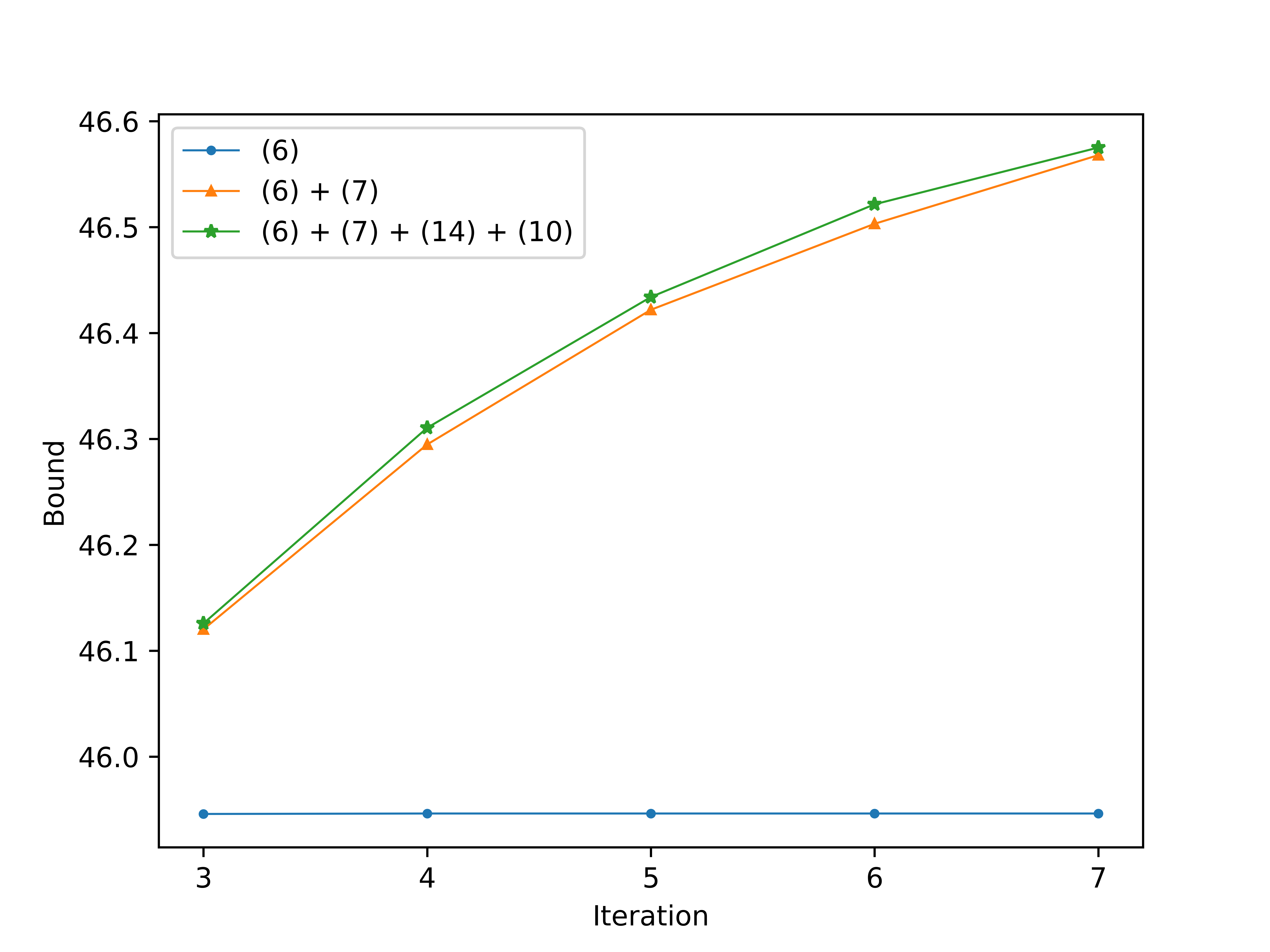
Figure 1: Evolution of the bound over the iterations of Algorithm 2,
Erdős-Rényi graph with $n=20$ and $p=0.8$, $7\text{ iterations}$

In Tables 1–4 we give the numerical results for the above mentioned instances, comparing our SDP bounds with those obtained when using an MILP solver. The column label $n$ refers to the number of vertices of the graph, $p$ and $d$ relates to the edges of the graph as specified in Section 4.2 above.

In Tables 1 and 3 columns “LB init” list the lower bounds obtained when solving the initial basic SDP relaxation without any cutting planes, while in column “LB final” the lower bound we finally obtained is displayed. “UB” is the upper bound obtained through our heuristic and “gap final” is computed as $(\mathrm{UB}-\mathrm{LB})/\mathrm{UB}$, where LB is the final lower bound. In the column with the “time” label, we report the total time for obtaining our lower bound, and how this total time is split into solving the SDPs and separating the violated inequality and equality constraints. Moreover, the time for computing the upper bound is given. The last column of these two tables indicate the number of cutting planes added when the algorithm stops. Tables 2 and 4 give the details when using CPLEX to obtain an (approximate) solution.

In the tables we see that adding the valid inequalities and equalities significantly improves the initial bound, in Table 1 the value of the bound increases by roughly 30%, for the random geometric graphs (Table 3) it is around 20 to 30%. Also the upper bounds we obtained are of good quality, overall the gap between our final lower bounds and the upper bounds is from 30% to 46% for the Erdős-Rényi graphs and between 27% and 53% for the random geometric graphs.

The time spent to compute the lower bounds ranges from a few seconds for the instances with 20 vertices up to 115 minutes for instances with 50 vertices. For the small instances, solving the SDPs can be done rather quickly and therefore, the time spent in the separation takes the bigger ratio. For larger instances, however, separating violated inequalities and equalities typically uses less than 20% of the overall time. Computing the upper bounds is done within less than 40 seconds.

We now turn our attention to comparing our results with using the MILP solver CPLEX, see Tables 2 and 4. As all our SDP based results are obtained within 2 hours, we set this as time limit for CPLEX. On small and sparse instances CPLEX performs very well. However, for the Erdős-Rényi graph with $n=40$ and 70% density we are left with a gap of 45% after two hours, compared to the gap of 34% that we obtain with our algorithm in less than 30 minutes. The random geometric graphs with $d$ equal to $0.3$ or $0.4$ can be solved for graphs with up to 40 vertices, for dense instances with at least $40$ vertices a gap of more than 35% remains after two hours run time. In general, the density has a huge impact on the runtime for the MILP solver. For example, it increases from 3.45 seconds for $p=0.3$ to 1206.53 seconds for $p=0.9$ for Erdős-Rényi graphs on 20 vertices. Our SDP based bounds do not show significant differences for sparse and dense instances for the Erdős-Rényi graphs, and only a minor increase of the runtime for the random geometric graphs.

To get a better understanding of the quality of our lower and upper bounds, we computed the optimal solutions for some instances by running the MILP-model up to several days of CPU-time. The results are displayed in Tables 6 and 6, in which the columns labeled $n$, $p$, $d$ and “density” relate to the same instance parameters as previously specified. Columns “LB” and “UB” list the lower and upper bounds, respectively, obtained by our algorithm. In column “opt” the optimal value of the CMP obtained with the MILP-model is given, and the last column shows the deviation of our lower bound from the optimum, i.e., the value $(\text{opt}-\text{LB})/\text{opt}$. These tables show that, for most of these instances, our upper bounds are rather close to the optimal value, and consequently that most of the gap comes from the lower bound. Indeed, the experiments show that our lower bound is always approximately 30% away from the optimum for the Erdős-Rényi graphs, and most of the time between 20% and 30% for the geometric graphs. As this behavior seems consistent, we can presume that it stays similar for the bigger and denser instances, for which we cannot compute the optimum in reasonable time. Another observation is that for the smallest instances the quality of the upper bound increases with the density of the graph, but it is unclear whether this is also the case for bigger instances.

Overall, the MILP approach is clearly outperformed by our method for dense graphs but also for graphs having 40 or 50 vertices, independent of their density.

Table 1: Bounds and times for the MCP using the SDP relaxation on Erdős–Rényi graphs

		bounds				time
		LB	LB		gap	LB	LB	LB
$n$	$p$	init	final	UB	final	total	SDP	sep.	UB	#cuts
20	0.3	10.99	14.27	26	0.42	62.62	23.37	38.28	0.36	3697
20	0.4	17.05	21.54	36	0.39	61.83	22.61	38.28	0.32	3826
20	0.5	17.14	21.92	41	0.46	63.94	23.47	39.40	0.44	3919
20	0.6	28.89	36.40	55	0.33	63.38	23.23	39.02	0.51	3832
20	0.7	30.59	38.65	57	0.32	63.59	23.37	39.20	0.39	3806
20	0.8	37.12	46.59	68	0.31	62.43	21.74	39.45	0.62	3789
20	0.9	46.87	59.47	88	0.32	59.05	19.58	38.37	0.49	3267
30	0.3	23.65	30.69	48	0.35	365.83	206.53	153.80	2.21	9364
30	0.4	32.20	41.79	76	0.45	370.88	212.26	153.67	1.67	9244
30	0.5	47.39	60.55	95	0.36	376.59	215.95	155.00	2.33	9687
30	0.6	55.72	70.84	101	0.30	400.35	235.57	158.45	3.01	10149
30	0.7	71.93	91.86	143	0.36	379.24	220.62	152.50	2.65	9160
30	0.8	86.47	110.58	168	0.34	401.19	237.39	156.08	4.33	8949
30	0.9	93.63	119.93	181	0.34	392.83	233.53	153.09	2.90	9106
40	0.3	46.15	60.12	92	0.34	1505.80	1092.75	396.12	4.97	17300
40	0.4	66.42	85.52	126	0.32	1597.97	1169.59	407.50	8.91	18712
40	0.5	77.24	99.75	155	0.35	1495.82	1091.20	387.26	5.41	16655
40	0.6	101.62	130.84	195	0.33	1593.94	1176.42	399.59	5.87	17849
40	0.7	120.73	155.30	235	0.34	1691.67	1271.61	397.09	10.94	17663
40	0.8	146.23	187.95	281	0.33	1723.79	1299.59	400.07	12.10	18293
40	0.9	176.23	227.74	346	0.34	1703.14	1291.81	391.63	7.64	16651
50	0.3	70.48	91.92	159	0.42	5310.93	4359.63	901.09	16.17	30416
50	0.4	102.90	133.61	211	0.36	5404.70	4436.08	905.93	28.63	30238
50	0.5	140.54	182.44	286	0.36	5313.71	4396.23	863.22	20.16	28586
50	0.6	170.81	221.14	338	0.34	5511.41	4594.26	858.48	24.56	28417
50	0.7	196.65	253.98	382	0.34	5552.34	4610.50	890.25	17.42	30954
50	0.8	241.24	312.20	468	0.33	6303.39	5365.25	881.05	22.80	29710
50	0.9	270.41	350.87	525	0.33	6033.16	5106.08	874.43	18.43	29418

Table 2: Bounds and times for the MCP using the MILP formulation on Erdős–Rényi graphs

$n$	$p$	LB	UB	gap	time
20	0.3	20.00	20	0.00	3.45
20	0.4	32.00	32	0.00	118.43
20	0.5	31.00	31	0.00	11.81
20	0.6	52.00	52	0.00	25.58
20	0.7	56.00	56	0.00	33.04
20	0.8	68.00	68	0.00	271.60
20	0.9	88.00	88	0.00	1206.53
30	0.3	44.00	44	0.00	191.15
30	0.4	60.00	60	0.00	203.37
30	0.5	87.00	87	0.00	1165.32
30	0.6	101.00	101	0.00	1326.97
30	0.7	123.33	136	0.09	7200.00
30	0.8	122.53	163	0.25	7200.00
30	0.9	134.75	176	0.23	7200.00
40	0.3	88.00	89	0.01	7200.00
40	0.4	115.37	121	0.05	7200.00
40	0.5	105.67	150	0.30	7200.00
40	0.6	117.00	193	0.39	7200.00
40	0.7	127.00	232	0.45	7200.00
40	0.8	143.80	283	0.49	7200.00
40	0.9	150.13	343	0.56	7200.00
50	0.3	91.44	142	0.36	7200.00
50	0.4	105.00	208	0.50	7200.00
50	0.5	106.09	283	0.63	7200.00
50	0.6	113.00	337	0.66	7200.00
50	0.7	123.93	388	0.68	7200.00
50	0.8	123.00	477	0.74	7200.00
50	0.9	128.42	536	0.76	7200.00

Table 3: Bounds and times for the MCP using the SDP relaxation on random geometric graphs

			bounds				time
			LB	LB		gap	LB	LB	LB
$n$	$d$	density	init	final	UB	final	total	SDP	sep.	UB	#cuts
20	0.3	0.18	4.66	5.24	9	0.33	42.55	7.02	34.74	0.26	2592
20	0.4	0.28	7.16	8.28	13	0.31	42.69	8.68	33.19	0.28	2439
20	0.5	0.42	13.03	16.50	24	0.29	61.18	20.23	40.03	0.32	3576
20	0.6	0.44	14.21	16.56	24	0.29	57.48	16.69	39.87	0.33	2989
20	0.7	0.72	33.23	39.83	67	0.40	58.37	17.32	39.80	0.64	3053
20	0.8	0.91	45.49	56.75	83	0.31	62.43	19.63	41.73	0.43	2955
20	0.9	0.83	39.93	48.57	69	0.29	59.91	19.82	39.07	0.41	2631
30	0.3	0.19	9.17	10.46	19	0.42	293.96	125.34	163.40	2.08	6305
30	0.4	0.35	26.04	32.72	65	0.49	337.93	167.22	165.32	2.14	8699
30	0.5	0.48	42.01	51.65	79	0.34	346.90	176.51	165.47	1.67	8342
30	0.6	0.75	76.20	92.20	136	0.32	373.08	198.05	167.51	4.28	7597
30	0.7	0.70	67.36	84.98	121	0.30	395.81	223.55	165.97	2.98	9897
30	0.8	0.94	105.86	134.97	200	0.32	391.51	219.12	166.81	2.27	8296
30	0.9	0.96	109.07	139.47	207	0.32	381.37	206.85	168.38	2.88	7682
40	0.3	0.21	18.42	22.48	34	0.32	1253.51	770.35	463.22	8.24	12957
40	0.4	0.31	30.87	39.98	61	0.34	1389.39	895.44	477.01	5.13	15569
40	0.5	0.44	55.25	69.41	149	0.53	1353.95	875.37	456.78	9.73	15999
40	0.6	0.55	80.26	97.37	135	0.27	1416.42	928.89	468.95	6.78	14286
40	0.7	0.74	131.38	165.83	234	0.29	1650.37	1178.59	453.00	6.85	17886
40	0.8	0.84	158.23	201.33	299	0.32	1669.65	1197.72	448.71	11.22	18253
40	0.9	0.95	190.22	245.12	363	0.32	1758.20	1290.30	448.63	7.24	17238
50	0.3	0.26	40.58	48.00	88	0.44	3534.43	2325.10	1157.76	18.29	18417
50	0.4	0.38	76.75	96.25	139	0.30	4139.52	2889.61	1197.40	18.88	22951
50	0.5	0.47	98.82	127.56	177	0.28	4433.95	3256.09	1128.30	15.79	26260
50	0.6	0.61	149.46	189.41	315	0.40	4604.08	3441.39	1109.84	19.08	27503
50	0.7	0.76	214.97	272.53	397	0.31	5064.41	3916.95	1089.12	24.48	28401
50	0.8	0.79	224.27	283.43	427	0.33	5512.39	4352.64	1086.82	38.97	29912
50	0.9	0.93	286.08	368.44	550	0.33	6983.07	5810.03	1118.61	20.22	31414

Table 4: Bounds and times for the MCP using the MILP formulation on random geometric graphs

$n$	$d$	LB	UB	gap	time
20	0.3	7.00	7	0.00	1.51
20	0.4	12.00	12	0.00	26.88
20	0.5	22.00	22	0.00	6.65
20	0.6	21.00	21	0.00	3.86
20	0.7	55.00	55	0.00	33.99
20	0.8	83.00	83	0.00	284.89
20	0.9	69.00	69	0.00	31.36
30	0.3	13.00	13	0.00	23.97
30	0.4	45.00	45	0.00	509.40
30	0.5	60.31	72	0.16	7200.00
30	0.6	126.00	126	0.00	1236.75
30	0.7	119.00	119	0.00	2401.15
30	0.8	107.80	200	0.46	7200.00
30	0.9	120.40	207	0.42	7200.00
40	0.3	31.00	31	0.00	1130.25
40	0.4	50.00	50	0.00	847.54
40	0.5	92.00	92	0.00	1241.06
40	0.6	119.31	126	0.05	7200.00
40	0.7	154.66	238	0.35	7200.00
40	0.8	166.00	294	0.44	7200.00
40	0.9	130.35	366	0.64	7200.00
50	0.3	57.64	63	0.09	7200.00
50	0.4	115.50	131	0.12	7200.00
50	0.5	146.40	175	0.16	7200.00
50	0.6	162.33	266	0.39	7200.00
50	0.7	146.67	398	0.63	7200.00
50	0.8	112.01	416	0.73	7200.00
50	0.9	115.90	556	0.79	7200.00

Table 5: Comparison of the SDP bounds with the optimal values for the MCP on Erdős–Rényi graphs

$n$	$p$	LB	UB	opt	$\frac{\text{opt}-\text{LB}}{\text{opt}}$
20	0.3	14.27	26	20	0.25
20	0.4	21.54	36	32	0.31
20	0.5	21.92	41	31	0.29
20	0.6	36.40	55	52	0.29
20	0.7	38.65	57	56	0.30
20	0.8	46.59	68	68	0.31
20	0.9	59.47	88	88	0.32
30	0.3	30.69	48	44	0.30
30	0.4	41.79	76	60	0.30
30	0.5	60.55	95	87	0.30
30	0.6	70.84	101	101	0.30
30	0.7	91.86	143	135	0.32
40	0.3	60.12	92	89	0.31
40	0.4	85.52	126	121	0.29
40	0.5	99.75	155	147	0.32

Table 6: Comparison of the SDP bounds with the optimal values for the MCP on geometric graphs

$n$	$d$	density	LB	UB	opt	$\frac{\text{opt}-\text{LB}}{\text{opt}}$
20	0.3	0.18	5.24	9	7	0.14
20	0.4	0.28	8.28	13	12	0.25
20	0.5	0.42	16.50	24	22	0.23
20	0.6	0.44	16.56	24	21	0.19
20	0.7	0.72	39.83	67	55	0.27
20	0.8	0.91	56.75	83	83	0.31
20	0.9	0.83	48.57	69	69	0.29
30	0.3	0.19	10.46	19	13	0.15
30	0.4	0.35	32.72	65	45	0.27
30	0.5	0.48	51.65	79	72	0.28
30	0.6	0.75	92.20	136	126	0.26
30	0.7	0.70	84.98	121	119	0.29
40	0.3	0.21	22.48	34	31	0.26
40	0.4	0.31	39.98	61	50	0.20
40	0.5	0.44	69.41	149	92	0.24

5 Conclusion and outlook

We presented an SDP based approach to compute lower and upper bounds on the cutwidth. In order to obtain tight bounds, we derive several classes of valid inequalities and equalities and a heuristic for separating those inequalities and equalities and add them iteratively in a cutting-plane fashion to the SDP relaxation. The solution obtained from the SDP relaxation also serves to compute an upper bound on the cutwidth. Our experiments show that we obtain high quality bounds in reasonable time. In particular, our method is by far not as sensitive to varying densities as MILP approaches.

As the number of vertices gets larger, solving the SDPs becomes the time consuming part and thus the bottleneck. This is due to the increasing size of the matrix, but even more due to the huge number of constraints. Therefore, in our future research we will investigate using alternating direction methods of multipliers (ADMM) instead of an interior-point method, as ADMM proved to be successful in solving SDPs with many constraints, see for example de Meijer et al. (2023). Also including our bounds in a branch-and-bound framework and thereby having an exact solution method is a promising future research direction.

In our experiments we observe that we were not able to push the gap significantly below $0.30$. We want to further investigate this to find theoretical evidence of this behavior. And finally, we want to apply our approach to computing related graph parameters, i.e., those that can also be formulated in terms of orderings of the vertices, like the treewidth or the pathwidth of a graph.

References

- Adams et al. [2015] Elspeth Adams, Miguel F Anjos, Franz Rendl, and Angelika Wiegele. A Hierarchy of subgraph projection-based semidefinite relaxations for some NP-hard graph optimization problems. INFOR. Information Systems and Operational Research, 53(1):40–47, 2015.
- Adams and Sherali [1986] Warren P. Adams and Hanif D. Sherali. A tight linearization and an algorithm for zero-one quadratic programming problems. Management Science, 32(10):1274–1290, 1986.
- Bodlaender [1986] Hans L. Bodlaender. Classes of graphs with bounded tree-width. Technical Report RUU-CS-86-22, Utrecht University, 1986.
- Bodlaender et al. [2012] Hans L. Bodlaender, Fedor V. Fomin, Arie M. C. A. Koster, Dieter Kratsch, and Dimitrios M. Thilikos. A note on exact algorithms for vertex ordering problems on graphs. Theory Comput. Syst., 50(3):420–432, 2012.
- Boisvert et al. [1997] Ronald F Boisvert, Roldan Pozo, Karin Remington, Richard F Barrett, and Jack J Dongarra. Matrix market: a web resource for test matrix collections. Quality of Numerical Software: Assessment and Enhancement, pages 125–137, 1997.
- Buchheim et al. [2010] Christoph Buchheim, Angelika Wiegele, and Lanbo Zheng. Exact algorithms for the quadratic linear ordering problem. INFORMS Journal on Computing, 22(1):168–177, 2010.
- Casel et al. [2019] Katrin Casel, Joel D. Day, Pamela Fleischmann, Tomasz Kociumaka, Florin Manea, and Markus L. Schmid. Graph and string parameters: connections between pathwidth, cutwidth and the locality number. In 46th International Colloquium on Automata, Languages, and Programming, volume 132 of LIPIcs. Leibniz Int. Proc. Inform., pages Art. No. 109, 16. Schloss Dagstuhl. Leibniz-Zent. Inform., Wadern, 2019.
- Christof and Löbel [1997] Thomas Christof and Andreas Löbel. PORTA: Polyhedron representation transformation algorithm. http://comopt.ifi.uni-heidelberg.de/software/PORTA/, 1997. Accessed: 2018-03-27.
- Chung and Seymour [1989] Fan R.K. Chung and Paul D. Seymour. Graphs with small bandwidth and cutwidth. Discrete Mathematics, 75(1-3):113–119, 1989.
- Coudert [2016a] David Coudert. A note on Integer Linear Programming formulations for linear ordering problems on graphs. PhD thesis, Inria; I3S; Universite Nice Sophia Antipolis; CNRS, 2016a.
- Coudert [2016b] David Coudert. Linear ordering problems on graphs. https://grafo.etsii.urjc.es/optsicom/cutwidth.htmlhttp://www-sop.inria.fr/members/David.Coudert/code/graph-linear-ordering.shtml, 2016b. Accessed: 2021-09-01.
- de Meijer et al. [2023] Frank de Meijer, Renata Sotirov, Angelika Wiegele, and Shudian Zhao. Partitioning through projections: Strong SDP bounds for large graph partition problems. Computers & Operations Research, 151:106088, 2023.
- Di et al. [1997] Giuseppe Di, Ashim Garg, Giuseppe Liotta, Roberto Tamassia, Emanuele Tassinari, and Francesco Vargiu. An experimental comparison of four graph drawing algorithms. Computational Geometry, 7(5-6):303–325, 1997.
- Díaz et al. [2002] Josep Díaz, Jordi Petit, and Maria Serna. A survey of graph layout problems. ACM Computing Surveys, 34(3):313–356, 2002.
- Fischer et al. [2019] Anja Fischer, Frank Fischer, and Philipp Hungerländer. New exact approaches to row layout problems. Mathematical Programming Computation, 11(4):703–754, 2019.
- Gaar [2020] Elisabeth Gaar. On different Versions of the Exact Subgraph Hierarchy for the Stable Set Problem. https://arxiv.org/abs/2003.13605, March 2020.
- Gaar and Rendl [2019] Elisabeth Gaar and Franz Rendl. A bundle approach for SDPs with exact subgraph constraints. In Andrea Lodi and Viswanath Nagarajan, editors, Integer Programming and Combinatorial Optimization, pages 205–218. Springer, 2019. ISBN 978-3-030-17953-3.
- Gaar and Rendl [2020] Elisabeth Gaar and Franz Rendl. A computational study of exact subgraph based SDP bounds for Max-Cut, stable set and coloring. Mathematical Programming, 183(1-2, Ser. B):283–308, 2020.
- Gaar et al. [2022] Elisabeth Gaar, Melanie Siebenhofer, and Angelika Wiegele. An SDP-based approach for computing the stability number of a graph. Mathematical Methods of Operations Research, 95(1):141–161, 2022.
- Giannopoulou et al. [2019] Archontia C. Giannopoulou, Michał Pilipczuk, Jean-Florent Raymond, Dimitrios M. Thilikos, and Marcin Wrochna. Cutwidth: obstructions and algorithmic aspects. Algorithmica, 81(2):557–588, 2019.
- Gruber and Rendl [2003] Gerald Gruber and Franz Rendl. Computational experience with stable set relaxations. SIAM Journal on Optimization, 13(4):1014–1028, 2003.
- Heggernes et al. [2011] Pinar Heggernes, Daniel Lokshtanov, Rodica Mihai, and Charis Papadopoulos. Cutwidth of split graphs and threshold graphs. SIAM Journal on Discrete Mathematics, 25(3):1418–1437, 2011.
- Heggernes et al. [2012] Pinar Heggernes, Pim van ’t Hof, Daniel Lokshtanov, and Jesper Nederlof. Computing the cutwidth of bipartite permutation graphs in linear time. SIAM Journal on Discrete Mathematics, 26(3):1008–1021, 2012.
- Hungerländer and Rendl [2013] Philipp Hungerländer and Franz Rendl. Semidefinite relaxations of ordering problems. Mathematical Programming, 140(1, Ser. B):77–97, 2013.
- IBM [2018] CPLEX Optimization Studio. IBM ILOG, 22.1.0 edition, 2018. Accessed 2022-04-04.
- Johnson et al. [1989] David S. Johnson, Cecilia R. Aragon, Lyle A. McGeoch, and Catherine Schevon. Optimization by simulated annealing: An experimental evaluation; part i, graph partitioning. Operations Research, 37(6):865–892, 1989.
- Kloeckner [2009] Benoît Kloeckner. Cutwidth and degeneracy of graphs. CoRR, abs/0907.5138, 2009.
- Korach and Solel [1993] Ephraim Korach and Nir Solel. Tree-width, path-width, and cutwidth. Discrete Applied Mathematics, 43(1):97–101, 1993.
- López-Locés et al. [2014] Mario C López-Locés, Norberto Castillo-García, Héctor J Fraire Huacuja, Pascal Bouvry, Johnatan E Pecero, Rodolfo A Pazos Rangel, Juan JG Barbosa, and Fevrier Valdez. A new integer linear programming model for the cutwidth minimization problem of a connected undirected graph. In Recent Advances on Hybrid Approaches for Designing Intelligent Systems, pages 509–517. Springer, 2014.
- Lovász and Schrijver [1991] László Lovász and Alexander Schrijver. Cones of matrices and set-functions and - optimization. SIAM Journal on Optimization, 1(2):166–190, 1991.
- Luttamaguzi et al. [2005] Jamiru Luttamaguzi, Michael Pelsmajer, Zhizhang Shen, and Boting Yang. Integer programming solutions for several optimization problems in graph theory. In 20th International Conference on Computers and Their Applications (CATA 2005), 2005.
- Martí et al. [2008] Rafael Martí, Vicente Campos, and Estefanía Piñana. A branch and bound algorithm for the matrix bandwidth minimization. European Journal of Operational Research, 186(2):513–528, 2008.
- Martí et al. [2013] Rafael Martí, Juan J. Pantrigo, Abraham Duarte, and Eduardo G. Pardo. Branch and bound for the cutwidth minimization problem. Comput. Oper. Res., 40(1):137–149, 2013.
- MOSEK ApS [2018] MOSEK ApS. MOSEK Optimization API for Python. Version 10.0. https://docs.mosek.com/latest/pythonapi/index.html., 2018. Accessed 2022-08-08.
- Pantrigo et al. [2010] Juan J Pantrigo, Rafael Martí, Abraham Duarte, and Eduardo G Pardo. Cutwidth minimization problem, Optsicom project. https://grafo.etsii.urjc.es/optsicom/cutwidth.html, 2010. Accessed: 2021-09-01.
- Raspaud et al. [1995] André Raspaud, Ondrej Sýkora, and Imrich Vrťo. Cutwidth of the de Bruijn graph. RAIRO Informatique Théorique et Applications. Theoretical Informatics and Applications, 29(6):509–514, 1995.
- Raspaud et al. [2009] André Raspaud, Heiko Schröder, Ondrej Sỳkora, Lubomir Torok, and Imrich Vrt’o. Antibandwidth and cyclic antibandwidth of meshes and hypercubes. Discrete Mathematics, 309(11):3541–3552, 2009.
- Rendl et al. [2021] Franz Rendl, Renata Sotirov, and Christian Truden. Lower bounds for the bandwidth problem. Computers & Operations Research, 135:105422, 2021.
- Santos and de Carvalho [2021] Vinícius Gandra Martins Santos and Marco Antonio Moreira de Carvalho. Tailored heuristics in adaptive large neighborhood search applied to the cutwidth minimization problem. European Journal of Operational Research, 289(3):1056–1066, 2021.
- Schwiddessen [2022] Jan Schwiddessen. A semidefinite approach for the single row facility layout problem. In Norbert Trautmann and Mario Gnägi, editors, Operations Research Proceedings 2021, pages 45–51. Springer International Publishing, 2022. ISBN 978-3-031-08623-6.
- Yannakakis [1985] Mihalis Yannakakis. A polynomial algorithm for the min-cut linear arrangement of trees. Journal of the ACM (JACM), 32(4):950–988, 1985.