Location and scale free tests for distinguishing between classes of distribution tails

Abstract

We consider the problem of distinguishing between two classes of distribution tails, under the assumption that tails from one class are lighter than tails from another. Except the distribution that we use for separating these two classes, we do not assume that the distributions belong to any of the maximum domains of attraction. Two tests are proposed: a scale free and a scale and location free, and their asymptotic properties are established. The efficiency of the developed tests in comparison with the tests proposed in the literature is examined on the basis of a simulation study. We also apply our tests to real data on human mortality at extreme age in US.

1 Introduction

Choosing the proper shape of distribution tail is an important and, at the same time, very delicate problem in modelling many phenomena. As an illustration let us mention here the long lasting discussion on the maximal human’s age, where the conclusion is very sensitive to the data considered and to the method of analysis (for more details see Section 4.4).

The majority of methods used in the statistical analysis of distribution tails is provided by extreme value theory and consists in the direct estimation of parameters of one of the general distribution tail models. Very popular are here the Gumbel block maxima method and the peak-over-threshold approach based on the Generalized Pareto Distribution (GPD) model, see dehaan , beirlantteugels , embrechts among others. Both methods assume that the distribution function $F$ is in the domain of attraction of some extreme value distribution, namely, for some sequences $a_{n}>0$ and $b_{n}$

$$F^{n}(a_{n}x+b_{n})\to EV_{\gamma}(x),\quad n\to\infty,$$

where

$$EV_{\gamma}(x)=\left\{\begin{array}[]{cc}\exp(-(1+\gamma x)^{-1/\gamma}),1+\gamma x>0,&\mbox{if }\gamma\neq 0,\\ \exp(-\exp(-x)),x\in\mathbb{R},&\text{if }\gamma=0.\end{array}\right.$$

These methods perform well for distributions from both the Fréchet ($\gamma>0$) and Weibull ($\gamma<0$) maximum domains of attraction (MDA). But these methods may not show good efficiency if tails of distributions belonging to the Gumbel MDA (i.e. if $\gamma=0$) are analyzed, see, for instance, Section 4.4. Indeed, if it is known that $\gamma=0,$ independently of the tail behavior of distribution nearby its right endpoint (note that in the Gumbel MDA there are so different in tail behavior distributions like normal and lognormal), the distribution tail is approximated by exponential distribution in the framework of GPD model (and by Gumbel distribution in the framework of the Gumbel block maxima method if we want to approximate the distribution of a sample maximum), see also discussion in Section 2.1. Next, both of these methods are based on the extreme value theorem, but the rate of convergence of the distribution of normalized maxima to the Gumbel distribution is usually very slow, resnick . Moreover, there are distributions that do not satisfy the conditions of the extreme value theorem (for example, distributions with super-heavy tails), which prevents the application of the mentioned methods.

Thus, there is a need to expand the standard methodology of statistics of univariate extremes by considering other models for distribution tails and thus to develop methods for distinguishing between such models. It is quite surprising that, to the best of our knowledge, there is no any general method proposed in the literature for this purpose. The present article is devoted to this problem.

For a cdf $F,$ denote $\overline{F}(x)=1-F(x),$ its tail distribution function, and $x^{\ast}_{F}:=\sup\{y:F(y)<1\},$ the right endpoint of $F$. Following resnick2 , we say that $\overline{F}$ and $\overline{G}$ are strictly tail-equivalent, if $x^{\ast}_{F}=x^{\ast}_{G}=:x^{\ast}$ and $\overline{F}(x)/\overline{G}(x)\to 1$ as $x\uparrow x^{\ast}$ (write $\overline{F}\sim\overline{G}$). We call the distribution tail the class of equivalence $T(\overline{F})$ of tail distribution functions, i.e. for all $\overline{G}$ the property $\overline{G}\sim\overline{F}$ is equivalent to $\overline{G}\in T(\overline{F}).$

Let $\textbf{X}_{n}=(X_{1},\ldots,X_{n})$ be i.i.d. random variables with a cdf $F,$ and $x_{F}^{\ast}=+\infty.$ In this work, we aim at proposing a location and scale free test for distinguishing between the hypothesis $H_{0}:T(\overline{F})\in A_{0}$ and the alternative $H_{1}:T(\overline{F})\in A_{1}$ (we write below $H_{0}:F\in A_{0}$ and $H_{1}:F\in A_{1},$ respectively, for simplicity, since the tail distribution function fully determines the distribution tail) by sample $\textbf{X}_{n}.$ Here $A_{0}$ and $A_{1}$ are two classes of distribution tails that are “separable” in some sense by some cdf $F_{0}$, in particular, all tails from $A_{0}$ are lighter (or heavier) than those from $A_{1}.$ We also propose a scale free test for distinguishing between $H_{0}$ and $H_{1},$ that is more powerful in some situations than the first one. It is worth noting that we do not assume that distributions with a tail from $A_{0}$ or $A_{1}$ belong to any of MDA, except $F_{0}$ in case $F_{0}\in A_{0}.$

The article is organized as follows. In Section 2.1, we discuss two recent models for distribution tails from the Gumbel MDA, namely, the Weibull type and log-Weibull type classes. The precursor of two tests proposed in the present paper is described in Section 2.2. Next, in Section 3.1 we introduce the notion of C-separability and provide examples of C-separable classes of distribution tails. A scale free and a location and scale free tests for distinguishing between C-separable classes of distribution tails are proposed in Sections 3.2 and 3.3, respectively, and their asymptotic properties are established, in particular, their consistency on the alternative. Using these tests one can distinguish between regularly varying, Weibull type and log-Weibull type distribution tails, although their applicability is certainly not limited to this. The problem of selection the optimal threshold level for testing hypotheses about distribution tails is concerned in Section 3.4. In Section 4, the performance of our methods is examined on both simulated and real data sets in comparison with methods considered in the literature. Proofs are postponed to Appendix.

2 Related work

2.1 Some recent models for distribution tails

In last two decades, several models for distribution tails were proposed that are not yet so actively used by practitioners. Firstly, let us pay attention on the model developed in devalk1 (see also the particular case of this model proposed in elmethni ). Following the description of this model in girard2020 , assume that the distribution tail of random variable $X$ (let $X\geq 1$ a.s. for simplicity) is given by

$$1-F(x)=\exp(-V^{\leftarrow}(\ln x)),\ x\geq 1,$$ (1)

where $V^{\leftarrow}(x):=\inf\{y:V(y)\geq x\}$ is the generalized inverse of $V(x)=\ln Q(1/\exp(x))$ with $Q,$ the quantile function of $F,$ that is $Q(t)=F^{\leftarrow}(1-1/t).$ It is also supposed that there exists a positive function $a,$ such that for all $t>0$

$$\lim_{x\to\infty}\frac{V(tx)-V(x)}{a(x)}=\frac{t^{\theta}-1}{\theta},$$ (2)

where for $\theta=0$ the right-hand side should be understood as $\ln t.$ Hence, $V$ is supposed to be of extended regular variation with index $\theta\in\mathbb{R},$ see for details dehaan . Note, that if $\theta>0$ then the parameter $\theta$ governs the tail behavior of the log-Weibull type distribution, i.e. having a cdf $F$ such that for all $t>0$

$$\lim_{x\to\infty}\frac{\ln(1-F(e^{tx}))}{\ln(1-F(e^{x}))}=t^{1/\theta}.$$ (3)

Representatives of this class are the lognormal distribution and the distributions with cdf $F(x)=1-\exp(-(\ln x)^{1/\theta}),x>1.$ If $0<\theta<1,$ then $F$ belongs to the Gumbel MDA; if $\theta=1,$ then it belongs to the Fréchet MDA (see Theorem 1, girard2020 ). The problems of estimation of the parameter $\theta,$ extreme quantiles and probabilities of rare events in the framework of this model are considered in devalk1 , girard2020 , devalk2 , devalk3 .

Another class of distributions from the Gumbel MDA that deserves attention is the class of Weibull type distributions, Girard , Goegebeur . Say that cdf $F$ is of Weibull type, if there exists $\theta>0$ such that for all $t>0$

$$\lim_{x\to\infty}\frac{\ln(1-F(tx))}{\ln(1-F(x))}=t^{1/\theta}.$$ (4)

The parameter $\theta$ is called the Weibull tail index. Representatives of this class are the normal, exponential, gamma, Weibull distributions among others. The model (1) as well as the GPD and EVD models does not provide good description for Weibull type distributions, since in (2) the parameter $\theta$ is equal to 0 for all distributions from this class as well as for distributions with lighter tails. The problems of estimation of the Weibull tail index and extreme quantiles for Weibull type distributions are investigated in elmethni , Girard , Bro , Beirlant , Gardes among others.

Hence, there is a need to develop methods for distinguishing between at least these 3 classes of distribution tails, namely, the classes of regularly varying, log-Weibull type and Weibull type distribution tails. There are many works devoted to the problem of distinguishing between distributions from the Gumbel and Fréchet MDA (see the review of such tests in hueslerpeng , nevesfraga ). However, the literature reveals an almost complete lack of work on distinguishing between distributions within the Gumbel MDA. In this respect we can only refer to Goegebeur , where the goodness-of-fit test for Weibull type behavior was proposed, and to R2 , R3 . To the best of our knowledge, the problem of goodness-of-fit testing for log-Weibull type behavior was not considered in the literature. Finally, we refer to R1 , where the simple test for distinguishing between two separable classes of distribution tails was proposed, that does not require the fulfillment of the extreme value theorem assumptions, see also the next section.

However, the statistics of the tests for distinguishing between distributions within the Gumbel MDA mentioned above are not invariant with respect to the scale and location parameter change, except the test by Goegebeur that is scale free. Inaccurate determination of the location and scale parameters when analyzing distribution tails can lead to serious errors in conclusions. Hence the problem of developing the location and scale free methods for statistical analysis of distribution tails is of undoubted interest.

The reason why these two models have not yet been widely adopted by practitioners may be that while the tail behavior of Weibull or log-Weibull type distribution is of interest, the Generalized Pareto model with $\gamma>0$ (or with $\gamma<0$ for Weibull type tail with $\theta<1$) may provide acceptable quality, whereas the approximation of the tail by exponential distribution may be much worse. This phenomena called the penultimate behavior was studied in cohen , penultimate for distributions from the Gumbel MDA. Later, these results were extended to other maximum domains of attraction in gomeshaan . Nevertheless, it was shown in gardesgirard2 that the extreme quantile estimator for Weibull type distributions based on the Weibull type model performs much better than the estimator based on the GPD model. It emphasizes once again that our methodology makes sense.

2.2 Initial test

Following R1 , we say that cdfs $H$ and $G$ with $x_{H}^{\ast}=x_{G}^{\ast}=:x^{\ast}$ satisfy the condition $B(H,G)$ (B-condition), if for some $\varepsilon\in(0,1)$ and $x_{0}$

$$\frac{(1-H(x))^{1-\varepsilon}}{1-G(x)}\text{ does not increase as }\ x>x_{0}.$$ (5)

It is easy to see that under this condition the tail of $H$ is lighter than the tail of $G,$ that is $\overline{H}(x)/\overline{G}(x)\to 0$ as $x\uparrow x^{\ast}.$ Let us call classes of distribution tails $A_{0}$ and $A_{1}$ $B$-separable, if there is a cdf $F_{0}$ such that for all $G\in A_{0}$ the condition $B(G,F_{0})$ holds and for all $H\in A_{1}$ the condition $B(F_{0},H)$ holds for some (maybe different) $\varepsilon$ and $x_{0}.$

Assume that the classes $A_{0}$ and $A_{1}$ are $B$-separable via $F_{0},$ and all distributions belonging to $A_{0}$ or $A_{1}$ are continuous. In R1 , the test for distinguishing between $H_{0}:F\in A_{0}$ and $H_{1}:F\in A_{1}$

$$\text{if }R_{k,n}>1+\frac{u_{1-\alpha}}{\sqrt{k}},\text{ then reject }H_{0},$$ (6)

was proposed, where $u_{1-\alpha}$ is the $(1-\alpha)$-quantile of the standard normal distribution $N(0,1)$ and

$$R_{k,n}=\ln(1-F_{0}(X_{(n-k)}))-\frac{1}{k}\sum\limits_{i=n-k+1}^{n}\ln(1-F_{0}(X_{(i)})),$$

where $X_{(1)}\leq\ldots\leq X_{(n)}$ denote the order statistics of a sample $\{X_{i}\}_{i=1}^{n}.$ It was shown in R1 , that the latter test has asymptotically the significance level $\alpha$ and is consistent on $H_{1},$ if $k\to\infty,$ $k/n\to 0$ as $n\to\infty.$ Later, in Kogut , it was shown that under some additional conditions the test (6) can be applied for distinguishing between classes of distribution tails that are not necessarily continuous.

If for some cdf $F_{0}$ the condition $B(F_{0},G)$ holds for all $G\in A_{0}$ and the condition $B(H,F_{0})$ holds for all $H\in A_{1}$ for some (maybe, different) $\varepsilon$ and $x_{0},$ then the following rule for testing the hypothesis $H_{0}:F\in A_{0}$ against the alternative $H_{1}:F\in A_{1}$ can be proposed

$$\text{if }R_{k,n}<1+\frac{u_{\alpha}}{\sqrt{k}},\text{ then reject }H_{0}.$$

Note, that this test can be applied even for distributions that do not satisfy the assumptions of the extreme value theorem. Using the test (6), one can distinguish between the tails of Weibull type and log-Weibull type distributions, heavy-tailed and light-tailed distributions, regularly varying and super-heavy tailed distributions among others. Weakness of conditions imposed on distributions and breadth of application makes this test a suitable method for choosing a model in the case, when nothing is known in advance about the heaviness of the tails. However, changing the scale and location parameters of $F_{0}$ and $F$ can lead to completely opposite results when using this test. The present work corrects this disadvantage.

3 Main results

3.1 $C$-condition and $C$-separability. Examples.

Hereinafter we assume that all considered distributions are continuous and their right endpoints are infinite. The methods proposed in this work can be extended on case of finite right endpoints, but this is beyond the scope of our paper. Denote the quantile function of $F$ by $u_{F}(t).$ Let us introduce the conditions that we use to establish the asymptotical properties of the tests proposed in this work.

Definition 1

Two cdfs $H$ and $G$ are said to satisfy the condition $C_{\delta}(H,G)$ ($C$-condition), if for some $\delta\geq 0$ there exists $t_{0}$ such that for all $t>t_{0}$ and $c>1$

$$\frac{u_{H}\big{(}c^{1+\delta}t\big{)}}{u_{G}(ct)}\leq\frac{u_{H}(t)}{u_{G}(t)}.$$ (7)

Note that if two cdfs $H$ and $G$ satisfy the condition $C_{0}(H,G)$ ($C_{0}$-condition), then starting from some $t_{0}$ the ratio $u_{H}(t)/u_{G}(t)$ does not increase. Clear, the condition $C_{\delta}(H,G)$ is weaker than the condition $C_{\delta^{\prime}}(H,G)$ for $\delta^{\prime}>\delta\geq 0.$

Next, it is easy to see that the condition $C_{\delta}(H,G)$ are invariant with respect to changes of the scale parameters of both $G$ and $H.$ However, these conditions may be violated in case of substituting $\sigma_{1}u_{H}(t)+a_{1}$ and $\sigma_{2}u_{H}(t)+a_{2}$ for $u_{H}(t)$ and $u_{G}(t),$ respectively, but this fact does not prevent us to prove the results of the next sections.

Let us show that the condition $C_{\delta}(H,G)$ implies the one similar to (5) that we will use in the proofs of the main results.

Proposition 1

Assume that cdfs $H$ and $G$ satisfy the condition $C_{\delta}(H,G)$ for some $\delta\geq 0$ and $t_{0}.$ Then for all $t>t_{0}$ and $c>1$

$$\frac{\big{(}1-H(cu_{H}(t))\big{)}^{1-\varepsilon}}{(1-H(u_{H}(t)))^{1-\varepsilon}}\leq\frac{1-G(cu_{G}(t))}{1-G(u_{H}(t))},$$ (8)

with $\varepsilon=1-(1+\delta)^{-1}.$

Proof

First, the continuity of $G$ and infinity of its right endpoint imply that for all $c>1$ there is $\tilde{c}>1,\tilde{c}=\tilde{c}(t),$ such that $c=u_{G}(\tilde{c}t)/u_{G}(t).$ From $C_{\delta}(H,G)$ it follows

$$u_{H}(t)\geq u_{G}(t)\frac{u_{H}\big{(}\tilde{c}^{1+\delta}t\big{)}}{u_{G}(\tilde{c}t)}.$$

Using this relation, we derive

$$\frac{\big{(}1-H(cu_{H}(t))\big{)}^{1-\varepsilon}}{1-G(cu_{G}(t))} = \frac{\left(1-H\Big{(}\frac{u_{G}(\tilde{c}t)}{u_{G}(t)}u_{H}(t)\Big{)}\right)^{1-\varepsilon}}{1-G(u_{G}(\tilde{c}t))}$$

$$\leq \frac{\left(1-H\Big{(}\frac{u_{G}(\tilde{c}t)}{u_{G}(t)}\frac{u_{H}(\tilde{c}^{1+\delta}t)}{u_{G}(\tilde{c}t)}u_{G}(t)\Big{)}\right)^{1-\varepsilon}}{1-G(u_{G}(\tilde{c}t))}$$

$$= \frac{\left(1-H(u_{H}(\tilde{c}^{1+\delta}t))\right)^{1-\varepsilon}}{1-G(u_{G}(\tilde{c}t))}=\frac{(\tilde{c}^{1+\delta}t)^{-(1-\varepsilon)}}{(\tilde{c}t)^{-1}}=t^{\varepsilon}$$

$$= \frac{(1-H(u_{H}(t)))^{1-\varepsilon}}{1-G(u_{G}(t))},$$

whence (8) follows.

Now we introduce the notion of $C$-separability.

Definition 2

Let $A_{0}$ and $A_{1}$ be two classes of distribution tails such that the tails belonging to the class $A_{0}$ are lighter than those from the class $A_{1}.$ We call $A_{0}$ and $A_{1}$ $C$-separable (from the right), if there exists a cdf $F_{0}$ such that for all $G\in A_{0}$ the condition $C_{0}(G,F_{0})$ holds for some (maybe different) $t_{0},$ and for all $H\in A_{1}$ the condition $C_{\delta}(F_{0},H)$ holds for some (maybe different) $\delta>0$ and $t_{0}.$

If classes $A_{0}$ and $A_{1}$ are $C$-separable from the right via cdf $F_{0},$ we call them $C(F_{0})$-separable from the right.

Note that if we replace the $C_{0}$ and $C$-conditions with the $B$-condition in this definition, then we derive the definition of $B$-separability. If the distribution tails from $A_{0}$ are heavier then those from $A_{1},$ then we say that these two classes are $C(F_{0})$-separable (from the left), if for some cdf $F_{0}$ and all $G\in A_{0}$ the condition $C_{0}(F_{0},G)$ holds for some (maybe different) $t_{0},$ and for all $H\in A_{1}$ the condition $C_{\delta}(H,F_{0})$ holds for some (maybe different) $\delta$ and $t_{0}.$

$C$-separability is a quite weak condition that is satisfied for a wide range of classes of distribution tails. Let us provide several examples of $C$-separable classes of distribution tails.

Example 1

Let $A_{0}$ and $A_{1}$ be the classes of the tails of Weibull and log-Weibull type distributions, respectively (for definitions, see Section 2.1). Assume that all distribution functions with tails from the classes $A_{0}$ and $A_{1}$ are eventually differentiable. To distinguish between these two classes we recommend to select the following cdf

$$F_{0}(x)=(1-\exp\{-\exp\{b(\ln x)^{1/2}\}\})I(x>1)$$ (9)

for some constant $b>0.$ The proof of $C(F_{0})$-separability from the right of these classes under some technical condition is given in Appendix. The proof of their $C(F_{0})$-separability from the left is similar. The finite sample properties of several tests for distinguishing between $A_{0}$ and $A_{1}$ are compared by numerical experiments in Section 4.2.

Example 2

Let $A_{0}$ be the class of the tails of log-Weibull type distributions with $\theta<1,$ and $A_{1}$ be the class of regularly varying distribution tails. Recall that the Fréchet MDA consists of the distributions with regularly varying tails only, write $F\in\mathcal{D}(EV_{\gamma}),\ \gamma>0$ for such distribution functions. Assume again that all distribution functions with tails from the classes $A_{0}$ and $A_{1}$ are eventually differentiable. To distinguish between these two classes we recommend to select the following cdf

$$F_{0}(x)=1-\exp(-\exp(b\,\sqrt{\ln\ln x})\ln x),\quad x>e,$$ (10)

for some constant $b>0.$ Indeed, the tails of log-Weibull type distributions with $\theta<1$ are lighter than the tail of $F_{0},$ and the condition $C_{0}(G,F_{0})$ for $G\in A_{0}$ follows from (3) and the properties of regularly varying functions. On the other hand, the condition $C_{\delta}(F_{0},H)$ for $H\in\mathcal{D}(EV_{\gamma}),\gamma>0,$ and $\delta>0$ follows from (10) and the definition of regularly varying distribution. We do not provide the detailed proof of these facts, because they are technical and in many respects similar to the proofs of corresponding facts in Example 1. Therefore, the $C(F_{0})$-separability from the right condition holds in this case as well. The comparison by numerical experiments of performance of tests for distinguishing between these two classes is provided in Section 4.3.

Example 3

Let the class $A_{0}$ be such that $u_{G}(t)=\int_{1}^{t}f(x)/x\,dx$ for all $G\in A_{0},$ where $f$ is positive and $f(x)\to\infty$ as $x\to\infty.$ It is clear that $G$ is heavy tailed. Next, let $A_{1}$ be the class of the tails of absolutely continuous Weibull type distributions with $\theta<1$. Then the classes $A_{0}$ and $A_{1}$ are $C(F_{0})$-separable from the left by $F_{0},$ the cdf of the standard exponential distribution. We omit the proof of this fact, since it is similar to the proof of Example 1.

Example 4

Consider an one-parameter family of distributions $F\in\{G_{\theta},\theta\in\Theta\}$ such that for all $\theta_{1},\theta_{2}\in\Theta,$ $\theta_{1}<\theta_{2},$ the cdfs $G_{\theta_{1}}$ and $G_{\theta_{2}}$ satisfy the condition $C_{\delta}(G_{\theta_{1}},G_{\theta_{2}})$ for $\delta>0.$ Then it is easy to see that the classes $A_{0}=\{G_{\theta},\ \theta<\theta_{0}\}$ and $A_{1}=\{G_{\theta},\ \theta>\theta_{0}\}$ are $C(G_{\theta_{0}})$-separable from the right. Moreover, $A_{1}$ and $A_{0}$ are $C(G_{\theta_{0}})$-separable from the left.

3.2 Scale free test

Assume that classes $A_{0}$ and $A_{1}$ are $C(F_{0})$-separable from the right via some cdf $F_{0}$. In this section, we discuss the following test for distinguishing between the hypothesis $H_{0}:F\in A_{0}$ and the alternative $H_{1}:F\in A_{1},$

$$\text{if }\tilde{R}_{k,n}>1+\frac{u_{1-\alpha}}{\sqrt{k}},\text{ then reject }H_{0},$$ (11)

where

$$\tilde{R}_{k,n}=\ln\frac{k}{n}-\frac{1}{k}\sum_{i=n-k+1}^{n}\ln(1-F_{0}(u_{0}(n/k)X_{(i)}/X_{(n-k)})),$$ (12)

and $u_{0}(t)=u_{F_{0}}(t)$. Clear, the distribution of $\tilde{R}_{k,n}$ does not depend on the scale parameters of both $F_{0}$ and $F,$ thus the test (11) is scale free. If for some cdf $F_{0}$ classes $A_{0}$ and $A_{1}$ are $C(F_{0})$-separable from the left, then for testing $H_{0}:F\in A_{0}$ against $H_{1}:F\in A_{1}$ we will use the following rule

$$\text{if }\tilde{R}_{k,n}<1+\frac{u_{\alpha}}{\sqrt{k}},\text{ then reject }H_{0}.$$

In the following results the asymptotical properties of the test (11) are stated.

Theorem 3.1

Let $X_{1},\ldots,X_{n}$ be i.i.d. random variables with a cdf $F_{0}.$ Assume $F_{0}$ satisfies the von Mises condition of belonging to $\mathcal{D}(EV_{\gamma}),$ $\gamma\geq 0,$

$$\lim_{x\uparrow\infty}\frac{(1-F_{0}(x))F_{0}^{\prime\prime}(x)}{F_{0}^{\prime}(x)^{2}}=-\gamma-1.$$ (13)

Assume a sequence $k=k(n)$ is such that

$$k\to\infty,k/n\to 0\mbox{ as }n\to\infty.$$ (14)

Then

$$\sqrt{k}(\tilde{R}_{k,n}-1)\stackrel{{\scriptstyle d}}{{\rightarrow}}N(0,1),\qquad n\to\infty.$$

Theorem 3.2

Let $X_{1},\ldots,X_{n}$ be i.i.d. random variables with a cdf $F_{1}$. Assume $F_{0}$ satisfies (13) and a sequence $k=k(n)$ satisfies (14). If the condition $C_{\delta}(F_{0},F_{1})$ holds for some $\delta>0$, then

$$\sqrt{k}(\tilde{R}_{k,n}-1)\xrightarrow{P}+\infty,\qquad n\to\infty,$$

and if $C_{\delta}(F_{1},F_{0})$ holds for some $\delta>0$, then

$$\sqrt{k}(\tilde{R}_{k,n}-1)\xrightarrow{P}-\infty,\qquad n\to\infty.$$

Corollary 1

Assume the assumptions of Theorem 3.2. Let $X_{1}^{0},\ldots,X_{n}^{0}$ be i.i.d. random variables with the cdf $F_{0}.$ Denote the values of the statistic (12) built by samples $(X_{1}^{0},\ldots,X_{n}^{0})$ and $(X_{1},\ldots,X_{n})$ as $\tilde{R}_{k,n}^{0}$ and $\tilde{R}_{k,n}^{1},$ respectively. If the condition $C_{0}(F_{0},F_{1})$ holds, then for all $x>0$

$$P(\tilde{R}_{k,n}^{0}>x)\leq P(\tilde{R}_{k,n}^{1}>x);$$

if $C_{0}(F_{1},F_{0})$ holds, then for all $x>0$

$$P(\tilde{R}_{k,n}^{0}>x)\geq P(\tilde{R}_{k,n}^{1}>x).$$

Hence, by Theorem 3.1 and Corollary 1, the test (11) has asymptotically the significance level $\alpha,$ and its consistency follows directly from Theorem 3.2.

Remark 1

Despite the fact that the test (11) has asymptotically the significance level $\alpha$ and is consistent on $H_{1}$ for every cdf $F_{0}$ satisfying (13) and for which classes $A_{0}$ and $A_{1}$ are $C(F_{0})$-separable, for finite $n$ the choice of $F_{0}$ matters. However, the problem of optimal selection of $F_{0}$ is beyond the scope of this paper. This remark is related also to the test proposed in the next section. However, some practical recommendations can be given, see Section 4.1.

Remark 2

As it follows from the results of this section, if classes $A_{0}$ and $A_{1}$ are $C(F_{0})$-separable from the right and for all $G\in A_{0}$ the condition $C_{\delta}(G,F_{0})$ holds for some positive $\delta$ (clear, $F_{0}$ does not belong to $A_{0}$ in this case), then the test (11) will be conservative. Thus, if $A_{0}$ has a natural “left bound” $\tilde{F},$ i.e. for all $G\in A_{0}$ the condition $C_{0}(G,\tilde{F})$ holds, but $C_{\delta}(G,\tilde{F})$ does not necessary hold for any $\delta>0$, we recommend selecting $F_{0}=\tilde{F}$ to maximize the power of the tests.

3.3 Location and scale free test

The test proposed in the previous section as well as the tests mentioned at the end of Section 2.1 are not invariant with respect to the location parameter, that can restrict sufficiently their application in some situations, see, e.g., Fig. 4. In this section, we aim at proposing the test for distinguishing between separable classes of distribution tails, that is invariant with respect to both the scale and location parameters. For this purpose, let us consider the following statistic

$$\widehat{R}_{k,n}=\ln\frac{k}{n}-\frac{1}{k}\sum_{i=n-k+1}^{n}\ln\left[1-F_{0}\Big{(}u_{0}(n/k)+\frac{X_{(i)}-X_{(n-k)}}{X_{(n-k)}-X_{(n-2k)}}\big{(}u_{0}(n/k)-u_{0}(n/(2k))\big{)}\Big{)}\right].$$ (15)

The asymptotic properties of $\widehat{R}_{k,n}$ are stated in the following results.

Theorem 3.3

Assume the assumptions of Theorem 3.1. Then

$$\sqrt{k}(\widehat{R}_{k,n}-1)\stackrel{{\scriptstyle d}}{{\rightarrow}}N\Big{(}0,1+\frac{\gamma^{2}}{2(\gamma+1)^{2}(2^{\gamma}-1)^{2}}\Big{)},\qquad n\to\infty,$$

where the ratio on the right-hand side should be understood as $1/(2(\ln 2)^{2})$ for $\gamma=0.$

Theorem 3.4

Assume the assumptions of Theorem 3.2. If the condition $C_{\delta}(F_{0},F_{1})$ holds for some $\delta>0$ then

$$\sqrt{k}(\widehat{R}_{k,n}-1)\xrightarrow{P}+\infty,\qquad n\to\infty;$$

if $C_{\delta}(F_{1},F_{0})$ holds for some $\delta>0$ then

$$\sqrt{k}(\widehat{R}_{k,n}-1)\xrightarrow{P}-\infty,\qquad n\to\infty.$$

Corollary 2

Assume the assumptions of Theorem 3.2. Let $X_{1}^{0},\ldots,X_{n}^{0}$ be i.i.d. random variables with the cdf $F_{0}.$ Denote the values of statistic (15) built by samples $(X_{1}^{0},\ldots,X_{n}^{0})$ and $(X_{1},\ldots,X_{n})$ as $\widehat{R}_{k,n}^{0}$ and $\widehat{R}_{k,n}^{1},$ respectively. If $C_{0}(F_{0},F_{1})$ holds then for all $x>0$

$$P(\widehat{R}_{k,n}^{0}>x)\leq P(\widehat{R}_{k,n}^{1}>x);$$

if $C_{0}(F_{1},F_{0})$ holds then for all $x>0$

$$P(\widehat{R}_{k,n}^{0}>x)\geq P(\widehat{R}_{k,n}^{1}>x).$$

Denote for convenience

$$\sigma^{2}(\gamma)=1+\frac{\gamma^{2}}{2(\gamma+1)^{2}(2^{\gamma}-1)^{2}},\quad\gamma>0,$$

and set $\sigma^{2}(0)=1+1/(2(\ln 2)^{2}).$ As in the previous section, consider two classes $A_{0}$ and $A_{1}$ of distribution tails such that tails from $A_{0}$ are lighter than those from $A_{1},$ and assume that these classes are $C(F_{0})$-separable from the right, where $F_{0}\in\mathcal{D}(EV_{\gamma}).$ Let us propose the following test for the hypothesis $H_{0}:F\in A_{0}$

$$\text{if }\widehat{R}_{k,n}>1+\frac{\sigma(\gamma)u_{1-\alpha}}{\sqrt{k}},\text{ then reject }H_{0}.$$ (16)

Clear, this test is location and scale free by the definition of $\widehat{R}_{k,n}.$ Moreover, by Theorem 3.3 and Corollary 2 the proposed test has asymptotically the significance level $\alpha,$ and its consistency on the alternative $H_{1}:F\in A_{1}$ follows from Theorem 3.4. The test for distinguishing between $A_{0}$ and $A_{1}$ in case of their $C(F_{0})$-separability from the left can be proposed similarly to the previous section.

Remark 3

Assume $A_{0}$ and $A_{1}$ are $C(F_{0})$-separable from the right. Formally speaking, the tests (11) and (16) distinguish not the hypothesis $H_{0}:F\in A_{0}$ and alternative $H_{1}:F\in A_{1},$ but the more wide hypothesis $\hat{H}_{0}:F\in\hat{A}_{0}$ and alternative $\hat{H}_{1}:F\in\hat{A}_{1},$ where $\hat{A}_{0}$ consists of all (continuous) cdfs $G$ satisfying the condition $C_{0}(G,F_{0})$, and $\hat{A}_{1}$ consists of all (continuous) cdfs $H$ satisfying $C(F_{0},H).$

Remark 4

Notice that distributions belonging to either $A_{0}$ or $A_{1}$ (except the cdf $F_{0}$ in case $F_{0}\in A_{0}$) do not have to satisfy the assumptions of the extreme value theorem.

3.4 The choice of $k$

An important problem for practitioners that we have not addressed yet is how to choose the parameter $k$ optimally. Indeed, the number $k$ should not be too small since the more observations we use, the more accurate our conclusions are. On the other hand, it should not be too large because, roughly speaking, the tail may “end” earlier and our conclusions about tail behavior in this case will turn out to be incorrect.

As related to estimation of various parameters in the framework of statistics of extremes, there are a lot of papers in the literature devoted to the problem of optimal selection of $k.$ For instance, we refer to Dani and Section 5.4, Gomes2 , for the review of such methods for tail index estimation and to Marrod for those for extremal index estimation, respectively. These methods are most often based on either some empirical principles, like choosing the optimal value of estimator from some interval of stability of its values, or on optimization of some metrics (e.g., MSE), often with using bootstrap.

However, the methods of choosing $k$ proposed for some estimators in the framework of statistics of extremes are not suitable for this purpose when testing the hypotheses about distribution tails. Indeed, a test statistic quite often has a steady increasing or decreasing trend as $k$ increases, hence the stability interval method cannot be used, and almost never tends to a certain finite value, hence the method of optimizing some metric in the form that used for parameter estimation cannot be applied as well. As a rule, in papers devoted to testing hypotheses about distribution tails this question is omitted. Moreover, the most comprehensive review hueslerpeng to date of methods for testing hypotheses about distribution tails suggests that the optimal selection of $k$ is an open problem.

Nevertheless, judging by our observations, some regularities in the behavior of test statistics can be distinguished. As a rule, the test for hypothesis about distribution tail can be represented as follows

$$\mbox{ if }S(k)>u,\mbox{ then reject }H_{0},$$

where $S(k)$ is a statistic built by the $k$ largest order statistics of a sample, and $u$ is some constant independent of $k.$ For instance, all the tests considered in this article can be written in such a way. Moreover, if is often possible to ensure that the limit distribution of $S(k)$ does not depend on $k$ under null hypothesis (or for some “boundary” distributions, like in this article, see Theorems 3.1 and 3.3), where $k$ is an intermediate sequence, i.e. it satisfies (14). Let us consider just such a case. Then the three most common types of $S(k)$ behavior are possible as $k$ increases, and the type of this behavior does not change on different samples from the same distribution. Below we provide recommendations for testing the null hypothesis for these three types of $S(k)$ behavior:

1. $S(k)$ has a well expressed increasing trend, and its values get larger than $u$ almost immediately. In this case, $H_{0}$ should be rejected.

2. $S(k)$ has a well expressed decreasing trend, and its values get smaller than $u$ almost immediately. In this case, $H_{0}$ should not be rejected.

3. The values of $S(k)$ oscillate around $u$ for some interval of small values of $k.$ As a rule, there is no stability of the $S(k)$ values in this case. For this type of behavior the following method may be proposed: if the proportion of the $S(k)$ values on this interval, exceeding the $u$ level, is greater than the significance level, then $H_{0}$ should be rejected.

Of course, these recommendations are empirical, and the problem of selection of $k$ while testing hypotheses about distribution tails deserves a separate study. Possible solutions to this problem may be, for instance, the use of multiple hypothesis testing or sequential analysis.

4 Simulation study

In this section, we examine the efficiency of the proposed tests in comparison with some tests proposed in the literature by numerical modelling. Before this, we provide some practical recommendation on selecting the parameters of $F_{0}$ for better test performance. We also provide an example of application of our methods on real data set. For the latter purpose, the data from the International base of longevity idl is used, which was analyzed, in particular, in the resonance works dong and rootzen .

4.1 Practical recommendations on selecting the parameters of $F_{0}$

Discussing the selection of $F_{0}$ in Remarks 1 and 2, we noted that we do not provide the procedure for the optimal choice of $F_{0}$ (and, consequently, its parameters) in our article. Nevertheless, some practical recommendations can be given.

Note first, that the statistic of the scale and location free test does not depend on the choice of the scale and location parameters of $F_{0},$ and the statistic of the scale free test does not depend on the choice of the scale parameter of $F_{0},$ respectively, thus these parameters do not need to be chosen.

Next, assume classes $A_{0}$ and $A_{1}$ are $C(F_{0})$-separable from the right. If $A_{0}$ has a natural “left bound”, see Remark 2 for definition and, e.g., Examples 3, 4, then $F_{0}$ should be chosen equal to this bound. In this case the additional parameters do not need to be chosen as well.

If $A_{0}$ has not a natural “left bound”, like in Examples 1 and 2, it is enough to vary only one parameter to derive good quality of test procedure. For this aim we suggest to choose some “basic” distribution in $A_{0}$ quite close to $A_{1}$ (for example, in Section 4.2 we choose the distribution $\mathcal{W}(2/3,1)$ for this purpose) and select the shape parameter of $F_{0}$ in such a way that the average empirical type I error probability would be less than the significance level, but close to it.

Finally, we note that using of the scale and location free test is preferable in case of distinguishing between distributions from the Gumbel MDA since the location parameter can strongly affect the tail behavior for small sample sizes (see Figure 4). It is also worth noting that, given a fixed null hypothesis and alternative, the same separating cdf $F_{0}$ can be used for different sample sizes.

4.2 Distinguishing between Weibull and log-Weibull type distribution tails

As mentioned in Introduction, there is actually only one work, where the tests to distinguish between the Weibull type and log-Weibull type tails were proposed, we mean the work of Goegebeur and Guillou Goegebeur . They introduced the Jackson-type and Lewis-type goodness-of-fit tests for Weibull type tail behavior.

We will compare the performance of the tests (11) and (16) adapted for testing the hypothesis $H_{0}:F\in\mathcal{W}$ against the alternative $H_{1}:F\in\mathcal{LW},$ where $\mathcal{W}$ and $\mathcal{LW}$ are the classes of Weibull type and log-Weibull type distribution tails, respectively, with the performance of the Jackson-type and Lewis-type tests from Goegebeur . Note that according to Remark 3 we can include the distributions with tails heavier than those from $\mathcal{LW}$, in particular, regularly varying distributions, to the alternative hypothesis. As a separating cdf for the tests (11) and (16), we select $F_{0}$ given by (9) with $b$ equal to $1.8$ and $3.5,$ respectively. We examine the performance of the tests listed above on the following set of distributions, that mostly coincides with the set of distributions used in Goegebeur . First, we list the Weibull type distributions:

• The Weibull distribution $\mathcal{W}(\alpha,\lambda)$

  $$F(x)=1-\exp(-\lambda x^{\alpha}),\quad x>0;\alpha,\lambda>0.$$

  We set $(\alpha,\lambda)=(2/3,1).$

• The standard normal distribution $\mathcal{N}(0,1).$

• The gamma distribution $\Gamma(\alpha,\lambda)$ with density

  $$p(x)=\frac{\lambda^{\alpha}x^{\alpha-1}}{\Gamma(\alpha)}e^{-\lambda x},\quad x>0;\alpha,\lambda>0.$$

  We set $(\alpha,\lambda)=(0.25,1),\ (4,1).$

• The modified Weibull distribution $\mathcal{MW}(\alpha,c),$ defined as the distribution of the random variable $Y=X\ln X,$ where $X\sim\mathcal{W}(\alpha,c).$ We set $\alpha=c=1.$

• The extended Weibull model $\mathcal{EW}(\alpha,\beta)$

  $$F(x)=1-r(x)e^{-x^{\alpha}},\quad x>0,$$

  where $\alpha>0$ and $r(x)$ is regularly varying at infinity with index $\beta\in\mathbb{R}.$ We set $r(x)=(x+1)^{-1}$ and $\alpha=2.$

Now we list the log-Weibull type distributions and distributions with heavier tails that we use in this section:

• The lognormal distribution $\mathcal{LN}(\mu,\sigma)$ with density

  $$p(x)=\frac{1}{\sqrt{2\pi\sigma^{2}}x}\exp\left(-\frac{(\ln x-\mu)^{2}}{2\sigma^{2}}\right),\quad x>0,\,\mu\in\mathbb{R},\,\sigma^{2}>0.$$

  We set $\mu=0$ and $\sigma^{2}=1.$

• The log-Weibull distribution $\mathcal{LW}(\theta,c)$ with cdf

  $$F(x)=1-\exp(-(\ln(x/c))^{\theta}),\quad x>c,\theta,c>0,$$

  set $(\theta,c)=(1.5,1).$

• The general Pareto distribution $\mathcal{GPD}(\alpha,\sigma)$ with cdf

  $$F(x)=1-(1+\gamma x/\sigma)^{-1/\gamma},\quad x>0,\,\gamma,\sigma>0.$$

  We consider $(\gamma,\sigma)=(0.25,1),(0.5,1),(1,1),$ further we denote them by $P_{1},$ $P_{2}$ and $P_{3},$ respectively.

• The t-distribution $\mathcal{T}(n)$ with $n=3$ degrees of freedom.

For each distribution, we generated $1000$ samples of size $n=5000$ (as it was chosen in Goegebeur ) and computed the rejection rates of all tests for $k$ running from $10$ up to $1000$ in steps of $10.$

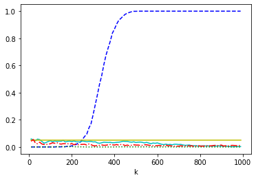
$\mathcal{W}(2/3,1)$

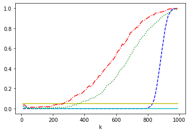
$\mathcal{N}(0,1)$

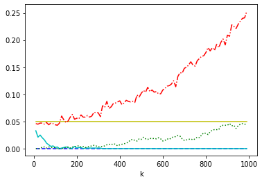
$\Gamma(0.25,1)$

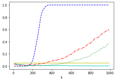
$\Gamma(4,1)$

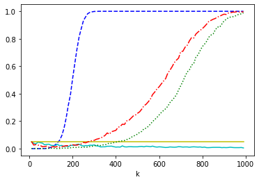
$\mathcal{MW}(1,1)$

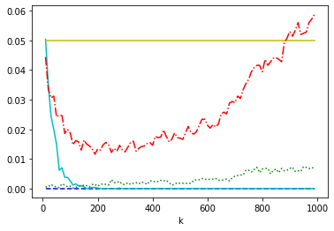
$\mathcal{EW}(2,-1)$

Figure 1: Empirical type I error probabilities of the tests (11) (blue dashed line), (16) (cyan solid line), Jackson-type (green dotted line) and Lewis-type (red dash-dotted line) tests for various distributions, the significance level $\alpha=0.05$ is indicated by yellow solid line, $n=5000.$

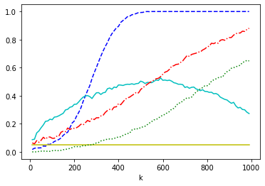
$\mathcal{LN}(0,1)$

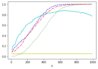
$\mathcal{LW}(1.5,1)$

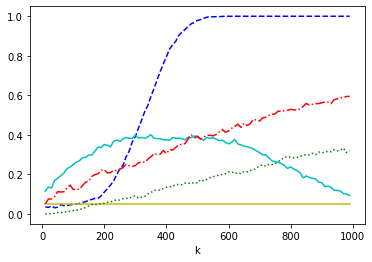
$\mathcal{GPD}(0.25,1)$

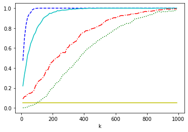
$\mathcal{GPD}(0.5,1)$

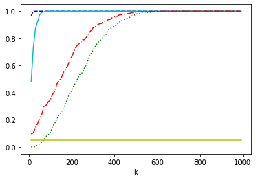
$\mathcal{GPD}(1,1)$

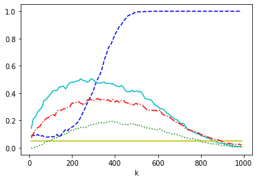
$\mathcal{T}(3)$

Figure 2: Empirical power of the tests (11) (blue dashed line), (16) (cyan solid line), Jackson-type (green dotted line) and Lewis-type (red dash-dotted line) tests for various distributions, the significance level $\alpha=0.05$ is indicated by yellow solid line, $n=5000$.

In Figs. 1-2 for the six null and six alternative distributions we plot the empirical rejection rates of the scale free test (11) (dashed line), location and scale free test (16) (solid line), Jackson-type test (dotted line) and Lewis-type test (dash-dotted line), proposed in Goegebeur , pointwise performed at the significance level 0.05, as functions of $k.$ We see, that the empirical rejection rates of only the test (16) are less than $0.05$ for all $k\leq 1000$ and distributions from the null hypothesis. However, one can note, that for small values of $k,$ namely $k\leq 250,$ the empirical I type error probabilities of all the compared tests, except (11), are less than $0.05$ on distributions from $H_{0}.$ We will pay our attention on this interval of $k$ values. Then, one can see that the test (16) is more powerful than the Jackson-type and Lewis-type tests and the test (11) is more powerful than the Lewis-type test on the distributions from the alternative as $k\leq 250.$

Analyzing Fig. 1-2, one may conclude that using the test (16) is always more preferable to the test (11). The reason of using (11) instead of (16), in particular, can be a small number of observations. It can also be reasonable to use (11) for distinguishing between quite heavy distribution tails (in particular, regularly varying), namely such that the location parameter does not greatly affect their behavior. In Fig. 3, we provide the empirical rejection rates of all tests considered in this section for distributions $\mathcal{LN}(0,1),$ $\mathcal{GPD}(0.25,1)$ and $\mathcal{T}(3).$ Here $n=1000,$ the significance level is $0.05$ and the number of samples is $m=1000.$ See, that the empirical power of (11) is substantially larger than the empirical power of other tests for moderate values of $k$.

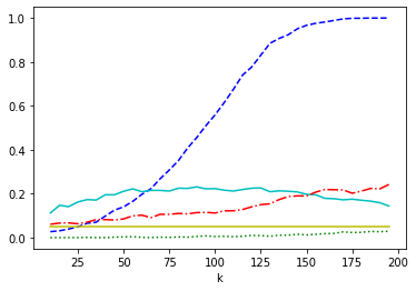
$\mathcal{LN}(0,1)$

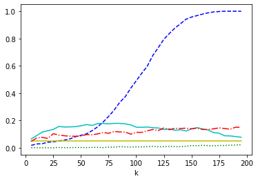
$\mathcal{GPD}(0.25,1)$

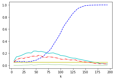
$\mathcal{T}(3)$

Figure 3: Empirical power of the tests (11) (blue dashed line), (16) (cyan solid line), the Jackson-type (green dotted line) and Lewis-type (red dash-dotted line) tests for various distributions, the significance level $\alpha=0.05$ is indicated by yellow solid line, $n=1000.$

However, it turns out that the Jackson-type and Lewis-type tests as well as the test (11) are quite sensitive to the location parameter change. In Fig. 4, we provide the empirical rejection rates of all the tests considered in this section for three exponential distributions with density $p(x)=\exp(-(x-a))I(x>a)$ and the values $a=-1,0,1$ of the location parameter, we set $n=5000,$ the significance level is $0.05$ and the number of samples is $m=1000.$ For $a=0$ the empirical type I error probabilities of all the tests are less than the significance level for all $k\leq 1000$ ($k\leq 800$ for the test (11)) whereas for $a=-1$ and $a=1$ the empirical type I error probabilities of all the tests except (16) increase substantially. Since even small changes of the location parameter cause the substantial changes in the statistical properties of the Jackson-type and Lewis type tests as well as the test (11), then these tests should be applied in practice with great caution in the lack of information about the location parameter. We also note that the Jackson-type and Lewis-type tests cannot be applied for samples containing, in particular, only negative observations, that is additional difficulty when using them.

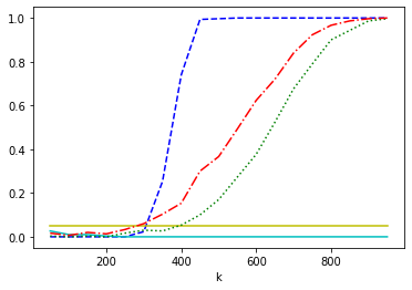
$Exp(1,-1)$

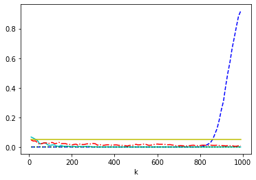
$Exp(1,0)$

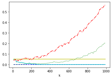
$Exp(1,1)$

Figure 4: Empirical power of the tests (11) (blue dashed line), (16) (cyan solid line), the Jackson-type (green dotted line) and Lewis-type (red dash-dotted line) tests for exponential distributions with various values of the location parameter, the significance level $\alpha=0.05$ is indicated by yellow solid line, $n=5000.$

4.3 Distinguishing between log-Weibull type and regularly varying distribution tails

In contrast to the previous section, the range of tests that can be used for the problem of this section is quite wide. In this section we consider the tests (11) and (16) adapted for distinguishing between the hypothesis $H_{0}:F\in\mathcal{LW}$ and alternative $H_{1}:F\in\mathcal{RV},$ where $\mathcal{RV}$ is the class of distributions with regularly varying tails that coincides with the Fréchet MDA $\mathcal{D}(EV_{\gamma}),\gamma>0$. We compare their efficiency with efficiency of some methods for testing the hypothesis $\tilde{H}_{0}:F\in\mathcal{D}(EV_{0}),$ i.e. the hypothesis of belonging to the Gumbel MDA, against the alternative $H_{1},$ we refer to nevesfraga for an overview of such methods. Namely, we use

1. the test proposed by Hasofer and Wang Hasofer-Wang , see also Alves-Neves , that is based on the Shapiro-Wilk type statistic

   $$W_{n}(k)=\frac{k\big{(}\frac{1}{k}\sum_{i=0}^{k-1}X_{(n-i)}-X_{(n-k+1)}\big{)}^{2}}{(k-1)\sum_{j=0}^{k-1}\big{(}\frac{1}{k}\sum_{i=0}^{k-1}X_{(n-i)}-X_{(n-j)}\big{)}^{2}};$$

2. the test proposed in Alves-Neves and based on the Greenwood type statistic $G_{n}(k),$ that is the modification of the previous test;

3. the ratio test proposed in Picek and based on the statistic

   $$R_{n}(k)=\frac{X_{(n)}-X_{(n-k)}}{\frac{1}{k}\sum_{i=0}^{k-1}X_{(n-i)}-X_{(n-k)}};$$

4. the likelihood ratio test, see e.g. Picek .

The numerical comparison of these tests can be found in Picek and Alves-Neves , see also nevesfraga .

As a separating cdf for the tests (11) and (16) we select $F_{0}$ given by (10) with $b$ equal to $0.6$ and $1.1,$ respectively. We compare the efficiency of these tests on the following distributions (many of which were introduced in the previous section) belonging to the Gumbel MDA:

• the standard exponential distribution $Exp(1);$

• the Weibull distribution $\mathcal{W}(2/3,1);$

• the gamma distribution $\Gamma(0.25,1);$

• the modified Weibull distribution $\mathcal{MW}(1,1);$

• the standard lognormal distribution $\mathcal{LN}(0,1);$

• the log-Weibull distribution $\mathcal{LW}(\theta,c)$ with $(\theta,c)=(1.5,1),(3,1).$

and to the Fréchet MDA:

• the generalized Pareto distribution $\mathcal{GPD}(\alpha,\sigma)$ with $(\gamma,\sigma)=(1/3,1),$
  $(0.5,1),(1,1),$ further we denote them by $P_{1},$ $P_{2}$ and $P_{3},$ respectively.

• the standard Cauchy distribution $\mathcal{C}(1);$

• the t-distribution with 3 degrees of freedom $\mathcal{T}(3);$

• The Burr distribution $Burr(c,d)$ with cdf

  $$F(x)=1-\frac{1}{(1+x^{-c})^{d}},\quad x>0.$$

  We select $(c,d)=(2,2),\,(3,2).$

For each distribution we generated $m=1000$ samples of size $n=5000,$ and computed the rejection rates of all tests for $k$ running from $10$ up to $1000$ in steps of $10.$ The empirical rejection rates of the Greenwood-type test were always a bit larger on the distributions used in this simulation study than the empirical rejection rates of the Hasofer-Wang test, hence we do not include the simulation results for the first test to the paper. By the same reason, we do not show the performance of the likelihood ratio test, which empirical properties are similar to those of the latter two tests.

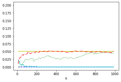
$Exp(1)$

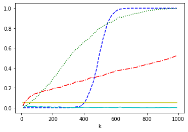
$\mathcal{W}(2/3,1)$

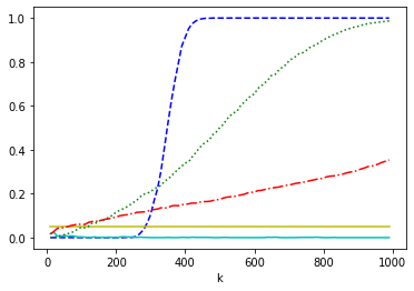
$\Gamma(0.25,1)$

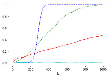
$\mathcal{MW}(1,1)$

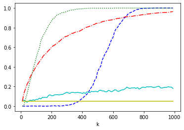
$\mathcal{LN}(0,1)$

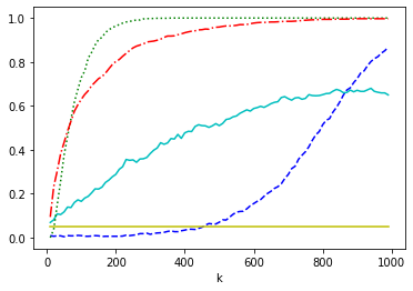
$\mathcal{LW}(1.5,1)$

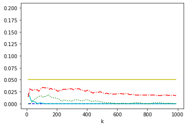
$\mathcal{LW}(3,1)$

Figure 5: Empirical type I error probabilities of the tests (11) (blue dashed line), (16) (cyan solid line), the Hasofer-Wang (green dotted line) and ratio (red dash-dotted line) for various distributions, the significance level $\alpha=0.05$ is indicated by yellow solid line, $n=5000.$

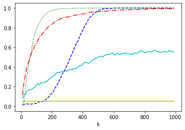
$\mathcal{GPD}(1/3,1)$

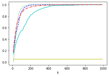
$\mathcal{GPD}(0.5,1)$

$\mathcal{GPD}(1,1)$

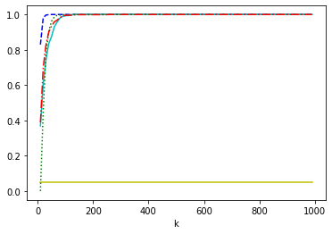
$\mathcal{C}(1)$

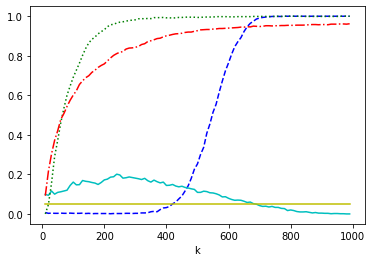
$\mathcal{T}(3)$

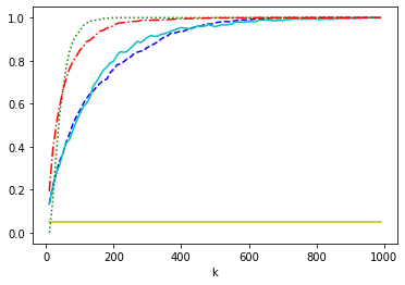
$Burr(2,2)$

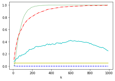
$Burr(3,2)$

Figure 6: Empirical power of the tests (11) (blue dashed line), (16) (cyan solid line), the Hasofer-Wang (green dotted line) and ratio (red dash-dotted line) tests for various distributions, the significance level $\alpha=0.05$ is indicated by yellow solid line, $n=5000.$

In Figs. 5–6 for the seven null and seven alternative distributions we plot the empirical rejection rates of the scale free test (11) (dashed line), location and scale free test (16) (solid line), Hasofer-Wang test (dotted line) and ratio test (dash-dotted line), pointwise performed at the significance level $0.05,$ as functions of $k.$

Note, that the empirical type I error probabilities of the Hasofer-Wang and ratio tests become greater than the significance level already for quite small values of $k$ for all the considered distributions from the null hypothesis, except $Exp(1)$ and $\mathcal{LW}(3,1).$ On the other hand, the empirical type I error probabilities of the test (16) exceed the significance level only for $\mathcal{LN}(0,1)$ and $\mathcal{LW}(1.5,1).$ However, even for these two distributions, they are much less than those of the Hasofer-Wang and ratio tests. This fact confirms that the test (16) is preferable in practice. We also note that the test (11) is conservative for all $k<200$ on all the considered distributions from the null hypothesis. But one should not forget that this test is only one in our comparison that is not location free.

If one takes a look on the figures where the empirical power of the tests on the alternative is shown, then one can make sure that all the tests show quite good efficiency. We indicate only not the best behavior of the tests proposed in this article for distributions $\mathcal{T}(3)$ and $Burr(3,2).$

Summarizing the results of this section, we can conclude, that the test (16) outperforms other tests considered in this section by empirical properties. Indeed, on the null hypothesis, this test makes mistakes much less often and is not much less powerful on the alternative. Apparently, this means that tests for the hypothesis $\tilde{H}_{0}:F\in\mathcal{D}(EV_{0})$ against the alternative $\tilde{H}_{1}:F\in\mathcal{D}(EV_{\gamma}),$ $\gamma>0,$ based on the tail heaviness are more efficient than tests based on the properties of the GEV and GPD models.

4.4 Real data example: analyzing human lifespan using IDL data

Analysis of the human lifespan has been long the subject of research by many scientists, see e.g. einmahl , belzile and references therein. However, until now, they have not come to a general agreement on whether there is a limit to the human lifespan. In the recent work dong , published in Nature, it is stated that “the maximum lifespan of humans is fixed and subject to natural constraints”. Rootzén and Zholud rootzen did not agree with the conclusions of the work dong . Based on the methods of statistics of extremes and the data provided by the International Database of Longevity (IDL, idl ), they concluded that the human lifespan distributions in many large regions (in particular, North America and West Europe among others) belong to the Gumbel MDA and have an infinite right endpoint. Nevertheless, for some smaller regions, the results of applying the methods of extreme value theory may be different; for example, in einmahl it was shown that the distribution of the human lifespan in the Netherlands belongs to the Weibull MDA and thus has a finite right endpoint.

Agreeing with the conclusions made in rootzen , we however want to pay the reader’s attention on Fig.5 (right) therein (see also Fig. 7 (left) in the present paper). In this figure, the empirical quantiles for IDL supercentenarians who died in 2000-2003 in USA (write the 2000-2003 US IDL data) and quantiles of the exponential distribution with mean estimated by the IDL lifespan data related to supercentenarians who died in 1980-1999 in USA are compared. This figure, in our opinion, reflects insufficient quality of approximation of this data by the exponential distribution, i.e. the special case of the GPD model at $\gamma=0,$ that is a clear illustration of conclusions made in Introduction. Below, we show that the approximation of the data ${\rm age}-110$ by the two-parameter Weibull distribution $\mathcal{W}(\alpha,\lambda)$ (for definition see Section 4.2) reflects the tail behavior of this data better. No doubts, it is not wondering since the exponential distribution is the special case of two-parameter Weibull distribution at $\alpha=1,$ but the point is that approximating the tails of all distributions from the Gumbel MDA by an exponential law can be inferior. It is also noted in rootzen that the deviation of this data from exponential distribution may be caused by the specific sampling scheme, but the specific processing of these data does not allow to take the information about the sampling scheme into account.

Hence, since we agree that the 2000-2003 US IDL data distribution belongs to the Gumbel MDA, let us first use the tests considered in Section 4.2 to find out which of the models: Weibull or log-Weibull type is suitable for describing this distribution. Note that for applying each of the four tests from Section 4.2, we should know $n,$ the number of deaths in USA in 2000-2003. One can find this information, in particular, on Wikipedia page wiki , namely $n=9771451.$ The number of supercentennarians in the 2000-2003 US IDL data is $k=504.$ The values of the scale free (11), location and scale free (16), Jackson-type and Lewis-type test statistics are $-10.64,\,-2.99,\,1.5$ and $1.34,$ respectively, and the $p$-values of these tests are $1,\,0.998,\,0.132$ and $0.18,$ respectively. Thus, we can conclude that the data distribution is of Weibull type. Indeed, from Fig. 5 right rootzen (see also Fig. 7, left) the tail of the 2000-2003 US IDL data distribution is lighter than the tail of exponential distribution.

Next, consider the exceedances of the data observations over the level $110,$ $y=age-110,$ and approximate them by the exponential distribution, as well as by the Weibull distribution $\mathcal{W}(\alpha,\lambda)$ and GPD model (in this case, we do not assume that $\gamma$ is necessarily equal to $0$), see Fig. 7, left. Specifically, we plot the points $(x,y),$ where $x$ always corresponds to quantiles of exponential distribution with mean estimated by the data and $y$ corresponds to empirical data quantiles and quantiles of the Generalized Pareto and Weibull distributions of the same level as $x$ with parameters estimated by the data. It is easy to see that the last two distributions fit the data better, that is especially noticeable for the largest observations of the sample. Note that the maximum likelihood estimate of the shape parameter $\alpha$ of $\mathcal{W}(\alpha,\lambda)$ is $1.21,$ whereas the values of the Weibull tail index estimators proposed by Beirlant , girard0 and Gardes , which evidently should be less than $1$ in this case (for $\mathcal{W}(\alpha,\lambda)$ the Weibull tail index is equal to $1/\alpha$), are $6.54,$ $5.95$ and $6.06,$ respectively. Apparently, this is caused by the fact that these estimators are not invariant with respect to the location parameter, that convinces of the need to develop location and scale free methods for estimating the Weibull tail index.

The better approximation by the Weibull distribution in comparison with the exponential distribution is maintained for the IDL lifespan data related to supercentenarians who died in 2005-2010 in USA as well, see Fig. 7, right; it is also seemed to be better than the approximation by the GPD model. It is interesting that the distribution tail of this data is even lighter than in the previous case. Indeed, the maximum likelihood estimate of the parameter $\alpha$ for $\mathcal{W}(\alpha,\lambda)$ is $1.42$ against $1.21$ in the previous case. The maximum likelihood estimate of the scale parameter of the exponential distribution is also changed from $1.51$ to $2.11,$ that perhaps indicates a change in the supercentenarian lifespan distribution.

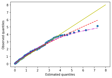
US supercentenarians in 2000-2003

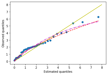
US supercentenarians in 2005-2010

Figure 7: Empirical quantiles for IDL supercentenarians who died in 2000–2003 (left) and in 2005-2010 (right) in USA (blue circles) plotted against quantiles of exponential (yellow solid line), Generalized Pareto (magenta dash-dotted line) and Weibull (red dashed line) distributions with parameters estimated by sample.

5 Appendix

5.1 Proof of Example 1

First let us show that for all $H\in A_{1}$ the condition $C_{\delta}(F_{0},H)$ holds for some $\delta>0$. We have $u_{F_{0}}(t)=\exp\big{(}(\ln\ln t/b)^{2}\big{)}.$ By its definition (3), the function $\ln(1-H(e^{t}))$ is regularly varying at infinity with index $1/\theta,$ $\theta>0,$ thus $1-H(t)=\exp\big{(}-(\ln t)^{1/\theta}\ell(\ln t)\big{)},t>1,$ for some slowly varying at infinity function $\ell(t).$ Therefore, by properties of slowly varying functions (see e.g. bingham ), there is a slowly varying function $\ell^{\sharp}(t)$ such that $u_{H}(t)=\exp\big{(}(\ln t)^{\theta}\ell^{\sharp}(\ln t)\big{)}.$

So, to check the condition $C_{\delta}(F_{0},H),$ we will show that for some $\delta>0$ there is $t_{0}$ such that for all $t>t_{0}$ the ratio

$$u_{F_{0}}(c^{1+\delta}t)/u_{H}(ct)=\exp\big{(}(\ln\ln(c^{1+\delta}t)/b)^{2}-(\ln(ct))^{\theta}\ell^{\sharp}(\ln(ct))\big{)}=\exp(f(c,t))$$

does not increase with respect to $c>1.$ For this purpose it is enough to show that the derivative with respect to $c$ of the function in the exponent on the right-hand side of the latter relation is negative for all $t>t_{0}$ and $c>1.$ Below we assume that the derivative of $\ell^{\sharp}$ is eventually monotone. Note that if the slowly varying function $\ell(t)$ is differentiable and its derivative is eventually monotone, then

$$\lim_{t\to\infty}t\ell^{\prime}(t)/\ell(t)=0,$$ (17)

see e.g. Theorem 1.7.2, bingham . Thus, for large $t_{0}$ we have

$$\frac{\partial f(c,t)}{\partial c}=\frac{1}{c}\cdot\frac{2(1+\delta)}{b^{2}}\cdot\frac{\ln\ln(c^{1+\delta}t)}{\ln(c^{1+\delta}t)}-\frac{1}{c}\theta(\ln(ct))^{\theta-1}\ell^{\sharp}(\ln(ct))(1+o(1))$$

$$<t\left(\frac{1}{ct}\cdot\frac{2(1+\delta)}{b^{2}}\cdot\frac{\ln\ln(ct)}{\ln(ct)}-\frac{1}{ct}\theta(\ln(ct))^{\theta-1}\ell^{\sharp}(\ln(ct))(1+o(1))\right)$$

$$=t\,\tilde{f}^{\prime}(ct),$$ (18)

with

$$\tilde{f}(x)=(1+\delta)((\ln\ln x)/b)^{2}-(\ln x)^{\theta}\ell^{\sharp}(\ln x).$$

It is easy to see that there is $x_{0}$ such that for all $x>x_{0}$ the derivative of $\tilde{f}(x)$ is negative. Selecting $t_{0}=x_{0},$ we finally derive by (18) that $\partial f(c,t)/\partial c<0$ for all $t>t_{0}$ and $c>1.$

Checking the condition $C_{0}(G,F_{0})$ for $G\in A_{0},$ where $A_{0}$ is the class of tails of Weibull type distributions, is much easier. Indeed, using properties of slowly varying functions and (4), we derive that $u_{G}(t)=(\ln t)^{\theta}\ell^{\sharp}(\ln t)$ for $\theta>0$ and some slowly varying $\ell^{\sharp}(t).$ Then we should show that the function

$$u_{G}(t)/u_{F_{0}}(t)=\exp\big{(}\theta\ln\ln t+\ln\ell^{\sharp}(\ln t)-((\ln\ln t)/b)^{2}\big{)}$$

does not increase eventually. Assuming again that the derivative of $\ell^{\sharp}$ is eventually monotone, we can show it by proving the fact that the derivative of the function in the exponent on the right-hand side of the latter relation is eventually negative. The latter fact follows immediately by using (17).

5.2 Proof of Theorem 3.1

We have,

$$\sqrt{k}(\tilde{R}_{k,n}-1)=\sqrt{k}(\tilde{R}_{k,n}-R_{k,n})+\sqrt{k}(R_{k,n}-1).$$

By Theorem 1, R1 ,

$$\sqrt{k}(R_{k,n}-1)\xrightarrow{d}N(0,1).$$ (19)

Thus, to complete the proof, it is enough to show that

$$\sqrt{k}(\tilde{R}_{k,n}-R_{k,n})\xrightarrow{P}0.$$

To prove this, we use the Chebyshev inequality for $\sqrt{k}(\tilde{R}_{k,n}-R_{k,n})$ given $X_{(n-k)}=q$ and full probability formula. For this purpose, we evaluate asymptotic of $\mathbb{E}(\tilde{R}_{k,n}-R_{k,n})$ and ${\rm Var}(\tilde{R}_{k,n}-R_{k,n})$ given $X_{(n-k)}.$

Explicit form of $\mathbb{E}(\tilde{R}_{k,n}-R_{k,n})$ given $X_{(n-k)}=q.$

We have,

$$\tilde{R}_{k,n}-R_{k,n} = \left(\ln\frac{k}{n}-\ln(1-F_{0}(X_{(n-k)}))\right)$$

$$-\frac{1}{k}\sum_{i=n-k+1}^{n}\ln\frac{1-F_{0}(u_{0}(n/k)X_{(i)}/X_{(n-k)})}{1-F_{0}(X_{(i)})}.$$

Consider the conditional distribution of $\tilde{R}_{k,n}-R_{k,n}$ given $X_{(n-k)}=q.$ By Lemma 3.4.1, dehaan , the joint conditional distribution of the set of order statistics $\{X_{(i)}\}_{i=n-k+1}^{n}$ given $X_{(n-k)}=q$ coincides with the (unconditional) joint distribution of the set of order statistics $\{X_{(i)}^{\ast}\}_{i=1}^{k}$ of i.i.d. random variables $\{X_{i}^{\ast}\}_{i=1}^{k}$ with common cdf

$$F_{q}(x)=P(X\leq x|X>q)=\frac{F_{0}(x)-F(q)}{1-F_{0}(q)},\ \ \ \ x>q.$$

Thus, given $X_{(n-k)}=q$,

$$\tilde{R}_{k,n}-R_{k,n}\stackrel{{\scriptstyle d}}{{=}}\left(\ln\frac{k}{n}-\ln(1-F_{0}(q))\right)-\frac{1}{k}\sum_{i=1}^{k}\ln\frac{1-F_{0}(u_{0}(n/k)X^{\ast}_{i}/q)}{1-F_{0}(X^{\ast}_{i})}.\;\;$$ (20)

Hereinafter we write $u_{0}$ instead of $u_{0}(n/k)$ for convenience. For $Y^{\ast}:=\ln(1-F_{0}(u_{0}X^{\ast}_{1}/q))-\ln(1-F_{0}(X^{\ast}_{1})),$ after direct, but tedious calculations, we derive

$$\mathbb{E}Y^{\ast}=\ln\frac{1-F_{0}(u_{0})}{1-F_{0}(q)}-(f(q)-1),$$ (21)

where

$$f(q)=\int_{q}^{\infty}\frac{u_{0}}{q}\frac{1-F_{0}(x)}{1-F_{0}(q)}\frac{p_{0}(u_{0}x/q)}{1-F_{0}(u_{0}x/q)}dx,$$ (22)

and $p_{0}(t)$ denotes a pdf of $F_{0}.$ This and (20) imply that

$$\mathbb{E}(\tilde{R}_{k,n}-R_{k,n}|X_{(n-k)}=q)=f(q)-f(u_{0})=f(q)-1.$$

Asymptotic of $\sqrt{k}\mathbb{E}(\tilde{R}_{k,n}-R_{k,n}|X_{(n-k)}).$

Next, show that

$$\sqrt{k}\mathbb{E}(\tilde{R}_{k,n}-R_{k,n}|X_{(n-k)})=\sqrt{k}(f(X_{(n-k)})-f(u_{0}))\xrightarrow{P}0.$$ (23)

As long as $F_{0}(u_{0}(x))=1-1/x,$ we have $p_{0}(u_{0}(x))u_{0}^{\prime}(x)=x^{-2}$ and $(xu^{\prime}_{0}(x))^{-1}=xp_{0}(u_{0}(x)).$ Then, Lemma 2.2.1, dehaan , implies

$$\frac{n}{\sqrt{k}}p_{0}(u_{0})(X_{(n-k)}-u_{0})\stackrel{{\scriptstyle d}}{{\rightarrow}}N(0,1).$$ (24)

Applying the delta method to the latter relation, we derive

$$\frac{n}{\sqrt{k}}p_{0}(u_{0})\frac{f(X_{(n-k)})-f(u_{0})}{f^{\prime}(u_{0})}\xrightarrow{d}N(0,1).$$ (25)

Generally speaking, this is not the classical delta method, since $u_{0}$ is not a constant and so the latter relation should be established. By the mean value theorem, we have $f(X_{(n-k)})-f(u_{0})=f^{\prime}(c)(X_{(n-k)}-u_{0})$ a.s., where $c$ is some (random) value between $X_{(n-k)}$ and $u_{0}.$ Thus it is enough to show that $f^{\prime}(c)/f^{\prime}(u_{0})\xrightarrow{P}1.$ The proof of this fact uses the explicit form of $f^{\prime}$ provided below and is based on the multiple application of the von Mises condition (13) and (24); it is very technical and is not of special interest. Thus here and in similar situations below we omit such technical details.

Next, calculating directly $f^{\prime}(q)$ and substituting $q=u_{0},$ we derive

$$f^{\prime}(u_{0})=\frac{n}{k}\bigg{(}p_{0}(u_{0})-\int_{u_{0}}^{\infty}\frac{x}{u_{0}}\frac{p^{2}_{0}(x)}{1-F_{0}(x)}dx\bigg{)}.$$

For absolutely continuous distributions with infinite right endpoint belonging to $\mathcal{D}(EV_{\gamma}),$ it holds

$$\frac{1-F_{0}(u)}{up_{0}(u)}\to\gamma,\quad u\to\infty,$$ (26)

see, e.g., Theorem 1.1.11, dehaan , for $\gamma>0$ and dehaan , p. 18, for $\gamma=0.$ Using the latter, L’Hospital rule and von Mises condition (13), we get

$$\lim_{u\to\infty}\frac{up_{0}(u)}{\int_{u}^{\infty}x\frac{p^{2}_{0}(x)}{1-F_{0}(x)}dx}=-\lim_{u\rightarrow\infty}\frac{up^{\prime}_{0}(u)+p_{0}(u)}{up^{2}_{0}(u)/(1-F_{0}(u))}$$

$$=-\lim_{u\rightarrow\infty}\frac{p^{\prime}_{0}(u)(1-F_{0}(u))}{(p_{0}(u))^{2}}-\lim_{u\rightarrow\infty}\frac{1-F_{0}(u)}{up_{0}(u)}=1,$$ (27)

whence

$$\frac{k}{np_{0}(u_{0})}f^{\prime}(u_{0})\xrightarrow{P}0.$$

Combining the latter and (25), we derive (23).

Asymptotic of ${\rm Var}(\tilde{R}_{k,n}-R_{k,n}|X_{(n-k)}).$

First, given $X_{(n-k)}=q$ we have,

$${\rm Var}(\tilde{R}_{k,n}-R_{k,n})=\frac{1}{k}{\rm Var}\left(\ln\frac{k}{n}-\ln(1-F_{0}(q))-Y^{\ast}\right)=\frac{1}{k}{\rm Var}Y^{\ast}.$$

Integrating by parts, we derive for the second moment of $Y^{\ast}$

$$\mathbb{E}(Y^{\ast})^{2}=\int_{q}^{\infty}\left(\ln\frac{1-F_{0}(u_{0}x/q)}{1-F_{0}(x)}\right)^{2}d\left(\frac{F_{0}(x)-F_{0}(q)}{1-F_{0}(q)}\right)=\left(\ln\frac{1-F_{0}(q)}{1-F_{0}(u_{0})}\right)^{2}$$

$$+2\int_{q}^{\infty}\ln\frac{1-F_{0}(u_{0}x/q)}{1-F_{0}(x)}\left(\frac{p_{0}(x)}{1-F_{0}(x)}-\frac{u_{0}}{q}\frac{p_{0}(u_{0}x/q)}{1-F_{0}(u_{0}x/q)}\right)\frac{1-F_{0}(x)}{1-F_{0}(q)}dx$$

$$=:\left(\ln\frac{1-F_{0}(q)}{1-F_{0}(u_{0})}\right)^{2}+2h(q).$$

From the latter and (21) it follows

$$\mathbb{E}(Y^{\ast})^{2}-(\mathbb{E}Y^{\ast})^{2}=2h(q)-2(f(q)-1)\ln\frac{1-F_{0}(q)}{1-F_{0}(u_{0})}-(f(q)-1)^{2}=:V(q).$$

Fix $\delta:$ $0<\delta<1/2.$ Let us show that

$$k^{2\delta}V(X_{(n-k)})\xrightarrow{P}0.$$ (28)

Note separately that $V(X_{(n-k)})=k{\rm Var}(\tilde{R}_{k,n}-R_{k,n}|X_{(n-k)}).$ Let $E_{1},\ldots,E_{n}$ be i.i.d. standard exponential and $E_{(1)}\leq E_{(2)}\leq\ldots\leq E_{(n)}$ be their order statistics. By continuity of $F_{0},$ we get $-\ln(1-F_{0}(X_{(n-k)}))\stackrel{{\scriptstyle d}}{{=}}E_{(n-k)},$ thus

$$-\sqrt{k}\ln\left(\frac{1-F_{0}(X_{(n-k)})}{1-F_{0}(u_{0})}\right)\stackrel{{\scriptstyle d}}{{=}}\sqrt{k}\big{(}E_{(n-k)}-\ln(n/k)\big{)}\xrightarrow{d}N(0,1),$$

by Lemma 2.2.1, dehaan . From the latter, (23) and the relation $f(u_{0})=1$ it follows

$$k^{2\delta}\left(2(f(X_{(n-k)})-1)\ln\frac{1-F_{0}(X_{(n-k)})}{1-F_{0}(u_{0})}+(f(X_{(n-k)})-1)^{2}\right)\xrightarrow{P}0.$$

Thus, to prove (28) it remains to show $k^{2\delta}h(X_{(n-k)})\xrightarrow{P}0.$ For this purpose we apply the delta method again. In this situation we cannot use the version of the delta method which we applied above since $h^{\prime}(u_{0})=0,$ thus we aim at finding the second derivative of $h(q)$ and substituting $q=u_{0}.$ Omitting tedious calculations, we derive

$$h^{\prime\prime}(u_{0})=\frac{1}{u_{0}^{2}(1-F_{0}(u_{0}))}\int_{u_{0}}^{\infty}\frac{x^{2}p^{3}_{0}(x)}{(1-F_{0}(x))^{2}}dx.$$

Note also that $h(u_{0})=0.$ From (24) and the relation $1-F_{0}(u_{0})=k/n$ we obtain

$$\frac{n^{2}}{k}\frac{p_{0}^{2}(u_{0})(h(X_{(n-k)})-h(u_{0}))}{2h^{\prime\prime}(u_{0})}=\frac{np_{0}^{2}(u_{0})h(X_{(n-k)})}{\int_{u_{0}}^{\infty}\frac{2x^{2}}{u_{0}^{2}}\frac{p_{0}^{3}(x)}{(1-F_{0}(x))^{2}}dx}\xrightarrow{d}\xi^{2},$$ (29)

where $\xi\sim N(0,1)$ and the asymptotics of the integral in the denominator follows from the L’Hospital rule, von Mises condition (13) and (26),

$$\lim_{u\to\infty}\frac{u^{2}p_{0}^{2}(u)/(1-F_{0}(u))}{\int_{u}^{\infty}2x^{2}\frac{p_{0}^{3}(x)}{(1-F_{0}(x))^{2}}dx}=\frac{1}{2}.$$

Substituting the latter to (29) and using the Slutsky theorem, we derive

$$kh(X_{(n-k)})\xrightarrow{d}\xi^{2}.$$

Therefore, for $\delta\in(0,1/2)$ it holds $k^{2\delta}h(X_{(n-k)})\xrightarrow{P}0,$ that proves (28).

Application of the Chebyshev inequality.

To complete the proof, show

$$\sqrt{k}(\tilde{R}_{k,n}-R_{k,n})-\sqrt{k}(f(X_{(n-k)})-f(u_{0}))\xrightarrow{P}0,$$ (30)

that, together with (23), implies the theorem. By the Chebyshev inequality, given $X_{(n-k)}=q,$ for all $\varepsilon>0$ we get

$$P\big{(}\sqrt{k}\big{|}(\tilde{R}_{k,n}-R_{k,n})-(f(q)-f(u_{0}))\big{|}>\varepsilon\big{)}\leq\frac{k{\rm Var}(\tilde{R}_{k,n}-R_{k,n})}{\varepsilon^{2}}.$$

By the latter and the full probability formula, we finally derive

$$P\left(\sqrt{k}|(\tilde{R}_{k,n}-R_{k,n})-(f(X_{(n-k)})-1)|>k^{\delta}\sqrt{V(X_{(n-k)})}\right)=$$

$$\int_{\mathbb{R}}P\left(\left.\sqrt{k}|(\tilde{R}_{k,n}-R_{k,n})-(f(X_{(n-k)})-1)|>k^{\delta}\sqrt{V(X_{(n-k)})}\right|X_{(n-k)}=q\right)\times$$

$$\times p_{X_{(n-k)}}(q)dq\leq\int_{\mathbb{R}}k^{-2\delta}p_{X_{(n-k)}}(q)dq=k^{-2\delta}\to 0,$$

where $p_{X_{(n-k)}}(q)$ is the pdf of $X_{(n-k)}.$ The result follows from (28).

5.3 Proof of Theorem 3.2

To prove Theorem 3.2, we need the following result.

Lemma 1

Let $X_{1}^{0},\ldots,X_{n}^{0}$ be i.i.d. random variables with common cdf $F_{0}.$ Then under the conditions of Theorem 3.2

$$\frac{1-F_{0}(cX^{0}_{(n-k)})}{1-F_{0}(X^{0}_{(n-k)})}-\frac{1-F_{0}(cu_{0})}{1-F_{0}(u_{0})}=O_{P}(1/\sqrt{k})$$ (31)

uniformly in $c>1.$

Proof

Applying the delta method for the function $f(x)=(1-F_{0}(cx))/(1-F_{0}(x))$ to the relation (24), we derive

$$\frac{n}{\sqrt{k}}p_{0}(u_{0})\frac{f(X^{0}_{(n-k)})-f(u_{0})}{f^{\prime}(u_{0})}\xrightarrow{d}N(0,1).$$

Thus to prove (31) it is enough to show that

$$\frac{\sqrt{k}}{n}\frac{f^{\prime}(u_{0})}{p_{0}(u_{0})}=O(1/\sqrt{k})$$ (32)

uniformly in $c>1.$ As long as

$$f^{\prime}(u_{0})=\left.\left(\frac{1-F_{0}(cx)}{1-F_{0}(x)}\right)^{\prime}\right|_{x=u_{0}}=\frac{p_{0}(u_{0})(1-F_{0}(cu_{0}))-cp_{0}(cu_{0})(1-F_{0}(u_{0}))}{(1-F_{0}(u_{0}))^{2}},$$

then using $1-F_{0}(u_{0})=k/n$ we can simplify the relation (32) as follows

$$\frac{1-F_{0}(cu_{0})}{1-F_{0}(u_{0})}-c\frac{p_{0}(cu_{0})}{p_{0}(u_{0})}=O(1)$$ (33)

uniformly in $c>1.$ Clear, $\overline{F}_{0}(cu_{0})/\overline{F}_{0}(u_{0})\leq 1$ for all $c>1.$ If $F_{0}\in\mathcal{D}(G_{\gamma})$ with $\gamma>0,$ boundness from above of the ratio $cp_{0}(cu_{0})/p_{0}(u_{0})$ follows from the Potter inequality, see, e.g., Proposition B.1.9, dehaan . If $\gamma=0,$ then the required fact follows from the relation (1.1.33), dehaan , that holds under (13), relation $p_{0}(u_{0}(t))u_{0}^{\prime}(t)=t^{-2}$ and Potter inequality again. Hence, the relation (33) and then the relation (31) hold. $\Box$

The proof of Theorem 3.2 repeats the proof of Theorem 2 (i) R1 in many respects. Namely, we will show that under the condition $C_{\delta}(F_{0},F_{1}),$ $\delta>0,$

$$\sqrt{k}(\tilde{R}_{k,n}-1)\gg\sqrt{k}\left(\frac{1}{k}\sum_{i=1}^{k}E_{i}-1\right)$$

for some i.i.d. random variables $\{E_{i}\}_{i\geq 1}$ with mean more than 1, and the result will follow from the central limit theorem. Here $X\gg Y$ means that $X$ is stochastically larger than $Y.$ The proof remains almost the same if $C_{\delta}(F_{1},F_{0})$ holds with $\delta>0$ instead of $C_{\delta}(F_{0},F_{1})$.

Let $X_{1},\dots,X_{n}$ be i.i.d. random variables with common cdf $F_{1}.$ Consider the asymptotic behavior of the statistic $\tilde{R}_{k,n}$ as $n\rightarrow\infty.$ Denote $Y_{i}=\ln(k/n)-\ln(1-F_{0}(u_{0}X^{\ast}_{i}/q)),$ $i=1,\ldots,k,$ where $\{X_{i}^{\ast}\}_{i=1}^{k}$ are i.i.d. random variables defined in the same way as in Theorem 3.1, with common cdf

$$F_{q}^{1}(x)=\frac{F_{1}(x)-F_{1}(q)}{1-F_{1}(q)},\ \ q<x.$$

By Lemma 3.4.1, dehaan , the joint distribution of the set of order statistics $\{Y_{(i)}\}_{i=1}^{k}$ of $\{Y_{j}\}_{i=1}^{k}$ coincides with the conditional joint distribution of the set of random variables $\{Z_{j}\}_{j=1}^{k}$ given $X_{(n-k)}=q,$ with

$$Z_{j}=\ln(k/n)-\ln(1-F_{0}(u_{0}X_{(n-j+1)}/X_{(n-k)})),\ j=1,...,k.$$

Clear, $\tilde{R}_{k,n}=\frac{1}{k}\sum_{j=1}^{k}Z_{j}.$ Thus, the conditional distribution of $\tilde{R}_{k,n}$ given $X_{(n-k)}=q$ coincides with the distribution of $\frac{1}{k}\sum_{i=1}^{k}Y_{i}.$ Therefore, we get

$$P(Y_{1}\leq x)=P(\ln(1-F_{0}(u_{0}X^{\ast}_{1}/q))\geq\ln(k/n)-x)=$$

$$P\big{(}X_{1}^{\ast}\leq qu_{0}^{-1}F_{0}^{\leftarrow}(1-ke^{-x}/n)\big{)}=\frac{F_{1}\big{(}qu_{0}^{-1}F_{0}^{\leftarrow}(1-ke^{-x}/n)\big{)}-F_{1}(q)}{1-F_{1}(q)}.$$ (34)

Next, cdfs $F_{1}$ and $F_{0}$ satisfy either the condition $C_{\delta}(F_{0},F_{1})$ or $C_{\delta}(F_{1},F_{0})$ with $\delta>0$ by assumptions. Assume that $C_{\delta}(F_{0},F_{1})$ holds with some $\delta>0$ and $t_{0},$ another case can be treated in a similar way. As long as $x^{\ast}=+\infty,$ $X_{(n-k)}\rightarrow+\infty$ almost surely, thus we can deal only with the case $n/k>t_{0}.$ Denote the quantile function of $F_{1}$ by $u_{1}(t)$ and write hereinafter $u_{1}$ instead of $u_{1}(n/k).$ By Proposition 1, we get

$$\frac{1-F_{1}(cu_{1})}{1-F_{1}(u_{1})}\geq\frac{(1-F_{0}(cu_{0}))^{1-\varepsilon}}{(1-F_{0}(u_{0}))^{1-\varepsilon}},\ \ c>1,$$ (35)

for some $\varepsilon>0.$

Denote $r=u_{1}^{\leftarrow}(q).$ Note also that if $X_{(n-k)}=u_{1}(\xi)$ for some random $\xi,$ then $u_{0}(\xi)\stackrel{{\scriptstyle d}}{{=}}X_{(n-k)}^{0}$ with $\{X_{i}^{0}\}_{i=1}^{n}$ introduced in Lemma 1. Proceed (34), using (35) with $c=u_{0}^{-1}F_{0}^{\leftarrow}(1-ke^{-x}/n)$ and (31). Uniformly in $x>0,$ we have

$$P(Y_{1}\leq x) = 1-\frac{1-F_{1}\big{(}u_{1}(r)u_{0}^{-1}F_{0}^{\leftarrow}(1-ke^{-x}/n)\big{)}}{1-F_{1}(u_{1}(r))}$$

$$\leq 1-\frac{\big{(}1-F_{0}(u_{0}(r)u_{0}^{-1}F_{0}^{\leftarrow}(1-ke^{-x}/n))\big{)}^{1-\varepsilon}}{\big{(}1-F_{0}(u_{0}(r))\big{)}^{1-\varepsilon}}$$

$$= 1-\left(\frac{1-F_{0}(F_{0}^{\leftarrow}(1-ke^{-x}/n))}{1-F_{0}(u_{0})}+O(1/\sqrt{k})\right)^{1-\varepsilon}$$

$$= 1-\left(e^{-x}+O(1/\sqrt{k})\right)^{1-\varepsilon}=1-e^{-(1-\varepsilon)x}+O(1/\sqrt{k}).$$

Since $O(1/\sqrt{k})$ vanishes, then for $k$ large enough there exists a cdf $G(x)$ such that

$$G(x)\geq\min(1-e^{-(1-\varepsilon)x}+O(1/\sqrt{k}),1)$$

with mean $(1-\varepsilon_{1})^{-1},$ $\varepsilon_{1}\in(0,\varepsilon),$ and variance $\sigma^{2}>0.$ Hence, $Y_{1}$ is stochastically larger than a random variable $E$ with cdf $G.$ Next, let $E_{1},\ldots,E_{k}$ be i.i.d. random variables with common cdf $G,$ then

$$\sqrt{k}\left(\frac{1}{k}\sum_{i=1}^{k}Y_{i}-1\right)\gg\sqrt{k}\left(\frac{1}{k}\sum_{i=1}^{k}E_{i}-1\right).$$ (36)

As long as (36) holds for all $q>x_{0},$

$$\sqrt{k}(\tilde{R}_{k,n}-1)\gg\sqrt{k}\left(\frac{1}{k}\sum_{i=1}^{k}E_{i}-1\right).$$ (37)

By the central limit theorem,

$$\sqrt{k}\left(\frac{1}{k}\sum_{i=1}^{k}E_{i}-\frac{1}{1-\varepsilon_{1}}\right)\xrightarrow{d}N(0,\sigma^{2}),$$

thus

$$\sqrt{k}\left(\frac{1}{k}\sum_{i=1}^{k}E_{i}-1\right)\xrightarrow{P}+\infty,$$

that with (37) completes the proof of Theorem 3.2.

5.4 Proof of Corollary 1

Let us assume that the condition $C_{0}(F_{0},F_{1})$ holds, the proof under the condition $C_{0}(F_{1},F_{0})$ is completely similar. The condition $C_{0}(F_{0},F_{1})$ immediately implies that

$$\frac{u_{0}(ct)}{u_{0}(t)}\leq\frac{u_{1}(ct)}{u_{1}(t)}$$ (38)

for all $c\geq 1$ and $t\geq t_{0}.$ As mentioned in the proof of Theorem 3.2, under the assumptions of Corollary 1 it holds $X^{0}_{1}\stackrel{{\scriptstyle d}}{{=}}u_{0}(u_{1}^{\leftarrow}(X_{1}))=:V_{1}.$ Hence substituting $t=u_{1}^{\leftarrow}(X_{(n-k)})$ and $c=u_{1}^{\leftarrow}(X_{(i)})/u_{1}^{\leftarrow}(X_{(n-k)})$ in (38), we get for all $i\in\{n-k+1,\ldots,n\}$

$$\frac{V_{(i)}}{V_{(n-k)}}=\frac{u_{0}(u_{1}^{\leftarrow}(X_{(i)}))}{u_{0}(u_{1}^{\leftarrow}(X_{(n-k)}))}\leq\frac{u_{1}(u_{1}^{\leftarrow}(X_{(i)}))}{u_{1}(u_{1}^{\leftarrow}(X_{(n-k)}))}=\frac{X_{(i)}}{X_{(n-k)}},$$ (39)

where $V_{(1)}\leq\ldots\leq V_{(n)}$ are the order statistics of i.i.d. random variables $\{V_{i}\}_{i=1}^{n},$ $V_{i}=u_{0}(u_{1}^{\leftarrow}(X_{i}))$ for $i\in\{1,\ldots,n\}.$ Since $(V_{(1)},\ldots,V_{(n)})\stackrel{{\scriptstyle d}}{{=}}\\ (X_{(1)}^{0},\ldots,X_{(n)}^{0}),$ then it follows from (39) that

$$\tilde{R}^{0}_{k,n} \stackrel{{\scriptstyle d}}{{=}} \ln\frac{k}{n}-\frac{1}{k}\sum_{i=n-k+1}^{n}\ln(1-F_{0}(u_{0}V_{(i)}/V_{(n-k)}))$$

$$\leq \ln\frac{k}{n}-\frac{1}{k}\sum_{i=n-k+1}^{n}\ln(1-F_{0}(u_{0}X_{(i)}/X_{(n-k)}))=\tilde{R}_{k,n},$$

the result follows.

5.5 Proof of Theorem 3.3

To prove Theorem 3.3, we need the following result.

Lemma 2

Let $E_{1},\ldots,E_{n}$ be i.i.d. standard exponential with $E_{(1)}\leq\ldots\leq E_{(n)},$ their order statistics. Then

$$\frac{n}{\sqrt{k}}\left(\left(\begin{array}[]{c}E_{(k)}\\ E_{(2k)}\end{array}\right)+\left(\begin{array}[]{c}\ln(1-k/n)\\ \ln(1-2k/n)\end{array}\right)\right)\xrightarrow{d}N\left(\Big{(}\begin{array}[]{c}0\\ 0\end{array}\Big{)},\Big{(}\begin{array}[]{cc}1&1\\ 1&2\end{array}\Big{)}\right),$$ (40)

if $k\to\infty,$ $k/n\to 0$ as $n\to\infty.$

Proof

The result of the lemma is almost the direct consequence of the following two-dimensional extension of Smirnov lemma smirnov , see also Lemma 2.2.3, dehaan . Let $U_{(1)}\leq\ldots\leq U_{(n)}$ be the $n$th order statistics from the standard uniform distribution. Then, if $k\to\infty,$ $k/n\to 0$ as $n\to\infty,$ the following relation holds

$$\left(\begin{array}[]{c}\frac{U_{(n-k)}-b_{n,k}}{a_{n,k}}\\ \frac{U_{(n-2k)}-b_{n,2k}}{a_{n,2k}}\end{array}\right)\xrightarrow{d}N\left(\Big{(}\begin{array}[]{c}0\\ 0\end{array}\Big{)},\Big{(}\begin{array}[]{cc}1&1/\sqrt{2}\\ 1/\sqrt{2}&1\end{array}\Big{)}\right),$$ (41)

where for $t\in\mathbb{N},$ $t<n$

$$b_{n,t}=\frac{n-t}{n-1},\quad a_{n,t}=\sqrt{\frac{1}{n-1}b_{n,t}(1-b_{n,t})}.$$

The proof of (41) is just a repetition of the proof of Lemma 2.2.3, dehaan . Firstly, the pdf of the random vector $(U_{(n-k)},U_{(n-2k)})$ is

$$\frac{n!}{((k-1)!)^{2}(n-2k)!}(1-x)^{k-1}(x-y)^{k-1}y^{n-2k},$$

thus the pdf of the vector $\big{(}(U_{(n-k)}-b_{n,k})/a_{n,k},\ (U_{(n-2k)}-b_{n,2k})/a_{n,2k}\big{)}$ is

$$\frac{n!}{((k-1)!)^{2}(n-2k)!}\,a_{n,k}\,a_{n,2k}(1-b_{n,k})^{k-1}(b_{n,k}-b_{n,2k})^{k-1}(b_{n,2k})^{n-2k}$$

$$\times\Big{(}1-\frac{a_{n,k}x}{1-b_{n,k}}\Big{)}^{k-1}\Big{(}1+\frac{a_{n,k}x-a_{n,2k}y}{b_{n,k}-b_{n,2k}}\Big{)}^{k-1}\Big{(}1+\frac{a_{n,2k}x}{b_{n,2k}}\Big{)}^{n-2k}.$$

By the Stirling formula one can conclude that the expression on the first line of the latter formula tends to $(\sqrt{2}\pi)^{-1},$ whereas the expression on the second line tends to

$$\exp(-x^{2}+\sqrt{2}xy-y^{2}).$$

Thus, (41) follows from the fact that pointwise convergence of the sequence of pdfs implies weak convergence of the probability distributions (Scheffe’s theorem).

Next, noticing that $a_{n,k}\sim a_{n,2k}/\sqrt{2}\sim\sqrt{k}/n$ and using the properties of multivariate normal distribution, we have

$$\frac{n}{\sqrt{k}}\left(\left(\begin{array}[]{c}U_{(n-k)}\\ U_{(n-2k)}\end{array}\right)-\left(\begin{array}[]{c}\frac{n-k}{n-1}\\ \frac{n-2k}{n-1}\end{array}\right)\right)\xrightarrow{d}N\left(\Big{(}\begin{array}[]{c}0\\ 0\end{array}\Big{)},\Big{(}\begin{array}[]{cc}1&1\\ 1&2\end{array}\Big{)}\right).$$ (42)

Finally, noticing that $(E_{(k)},E_{(2k)})\stackrel{{\scriptstyle d}}{{=}}(-\ln(U_{(n-k)}),-\ln(U_{(n-2k)})),$ we derive the result by the row-wise application of the delta method with function $f(x)=-\ln x$ to the last relation. Indeed, by the mean value theorem for the first and second rows in (42) we have

$$\frac{n}{\sqrt{k}}\left(\left(\begin{array}[]{c}E_{(k)}\\ E_{(2k)}\end{array}\right)+\left(\begin{array}[]{c}\ln(1-k/n)\\ \ln(1-2k/n)\end{array}\right)\right) \stackrel{{\scriptstyle d}}{{=}} \frac{n}{\sqrt{k}}\left(\begin{array}[]{c}f(U_{(n-k)})-f\big{(}\frac{n-k}{n-1}\big{)}\\ f(U_{(n-2k)})-f\big{(}\frac{n-2k}{n-1}\big{)}\end{array}\right)$$

$$= \frac{n}{\sqrt{k}}\left(\begin{array}[]{c}f^{\prime}(c_{1})\big{(}U_{(n-k)}-\frac{n-k}{n-1}\big{)}\\ f^{\prime}(c_{2})\big{(}U_{(n-2k)}-\frac{n-2k}{n-1}\big{)}\end{array}\right)$$

a.s., where $c_{i},$ $i=1,2,$ are some (random) values between $U_{(n-ik)}$ and $(n-ik)/(n-1),$ $i=1,2,$ respectively. But for $i=1,2$ $f^{\prime}(c_{i})=1/c_{i},$ $U_{(n-ik)}\to 1$ in probability and $(n-ik)/(n-1)\to 1,$ thus $f^{\prime}(c_{i})\to 1$ in probability. This and Slutsky theorem imply (40). $\Box$

The schemes of the proofs of Theorems 3.1 and 3.3, in fact, coincide. However, the proof of the latter is more difficult technically since the statistic $\widehat{R}_{k,n}$ depends on $X_{(n-k)}$ and $X_{(n-2k)}$ together. Moreover, if $\gamma>0$ then $\sqrt{k}(\widehat{R}_{k,n}-R_{k,n})$ will no longer tend to $0$ in probability.

Explicit form of $\mathbb{E}(\widehat{R}_{k,n}-R_{k,n})$ given $X_{(n-k)}=q$ and $X_{(n-2k)}=\hat{q}.$

Write $\sqrt{k}(\widehat{R}_{k,n}-R_{k,n})$ in explicit form

$$\sqrt{k}(\widehat{R}_{k,n}-R_{k,n})=\sqrt{k}\left(\ln\frac{k}{n}-\ln(1-F_{0}(X_{(n-k)}))\right)$$

$$-\frac{1}{\sqrt{k}}\sum_{i=n-k+1}^{n}\left[\ln\left(1-F_{0}\Big{(}u_{0}+\frac{X_{(i)}-X_{(n-k)}}{X_{(n-k)}-X_{(n-2k)}}(u_{0}-\hat{u}_{0})\Big{)}\right)-\ln(1-F_{0}(X_{(i)}))\right],$$

where $\hat{u}_{0}=u_{0}(n/(2k)),$ and consider its conditional distribution given $X_{(n-k)}=q$ and $X_{(n-2k)}=\hat{q}.$ Using the argument similar to the one from the proof of Theorem 3.1 and inheriting the notation from there, we get

$$\sqrt{k}(\widehat{R}_{k,n}-R_{k,n})\stackrel{{\scriptstyle d}}{{=}}\sqrt{k}\left(\ln\frac{k}{n}-\ln(1-F_{0}(q))\right)$$

$$-\,\frac{1}{\sqrt{k}}\sum_{i=1}^{k}\left[\ln\left(1-F_{0}\Big{(}u_{0}+\frac{X_{i}^{\ast}-q}{q-\hat{q}}(u_{0}-\hat{u}_{0})\Big{)}\right)-\ln(1-F_{0}(X_{i}^{\ast}))\right].$$ (45)

Hereinafter we write $\overline{F}(x)$ instead of $1-F(x).$ Denote

$$Y^{\ast}=\ln\overline{F}_{0}\Big{(}u_{0}+\frac{X_{1}^{\ast}-q}{q-\hat{q}}(u_{0}-\hat{u}_{0})\Big{)}-\ln\overline{F}_{0}(X_{1}^{\ast})$$

and find its mean. After integrating by parts, we derive

$$\mathbb{E}Y^{\ast}=\ln\frac{\overline{F}_{0}(u_{0})}{\overline{F}_{0}(q)}$$

$$-\int\limits_{q}^{\infty}\frac{\overline{F}_{0}(x)}{\overline{F}_{0}(q)}\left(\frac{u_{0}-\hat{u}_{0}}{q-\hat{q}}\frac{p_{0}\big{(}u_{0}+(u_{0}-\hat{u}_{0})(x-q)/(q-\hat{q})\big{)}}{\overline{F}_{0}\big{(}u_{0}+(u_{0}-\hat{u}_{0})(x-q)/(q-\hat{q})\big{)}}-\frac{p_{0}(x)}{\overline{F}_{0}(x)}\right)dx$$

$$=:\ln\frac{\overline{F}_{0}(u_{0})}{\overline{F}_{0}(q)}+1-f(q,\hat{q}).$$

from which and (45) we get

$$\mathbb{E}(\widehat{R}_{k,n}-R_{k,n}|X_{(n-k)}=q,X_{(n-2k)}=\hat{q})=f(q,\hat{q})-1.$$

Evaluating the asymptotic of $\sqrt{k}\mathbb{E}(\tilde{R}_{k,n}-R_{k,n}|X_{(n-k)},X_{(n-2k)}).$

Now find the asymptotic of

$$\sqrt{k}(f(X_{(n-k)},X_{(n-2k)})-1)=\sqrt{k}\mathbb{E}(\tilde{R}_{k,n}-R_{k,n}|X_{(n-k)},X_{(n-2k)}).$$

For this aim, in contrast to the proof of Theorem 3.1, we need the multivariate delta method. First of all, observe that

$$(X_{(n-k)},X_{(n-2k)})\stackrel{{\scriptstyle d}}{{=}}\left(u_{0}\Big{(}\frac{1}{1-\exp(-E_{(k)})}\Big{)},u_{0}\Big{(}\frac{1}{1-\exp(-E_{(2k)})}\Big{)}\right),$$

where the order statistics $E_{(k)}$ and $E_{(2k)}$ were introduced in Lemma 2. So, apply the multivariate delta method for the function

$$g(x,y)=f\left(u_{0}\Big{(}\frac{1}{1-e^{-x}}\Big{)},u_{0}\Big{(}\frac{1}{1-e^{-y}}\Big{)}\right)$$

to the relation (40). We get

$$\frac{\sqrt{k}\big{(}f(X_{(n-k)},X_{(n-2k)})-f(u_{0},\hat{u}_{0})\big{)}}{\frac{k}{n}\sqrt{D}}\xrightarrow{d}N(0,1),$$

where

$$D=\nabla g\left(\begin{array}[]{cc}1&1\\ 1&2\end{array}\right)(\nabla g)^{T}$$

and $\nabla g$ is the gradient of $g(x,y)$ at the point $(-\ln(1-k/n),-\ln(1-2k/n)).$ Observe also $f(u_{0},\hat{u}_{0})=1.$ Thus, one can see, that the asymptotic of $\sqrt{k}\mathbb{E}(\tilde{R}_{k,n}-R_{k,n}|X_{(n-k)},X_{(n-2k)})$ strongly depends on the asymptotic of $\frac{k}{n}\sqrt{D}.$ Let us show that

$$\frac{k}{n}\sqrt{D}\to\frac{1}{\sqrt{2}(2^{\gamma}-1)}\frac{\gamma}{\gamma+1},$$ (46)

where for $\gamma=0$ the right-hand side should be understood as $(\sqrt{2}\ln 2)^{-1}.$

Evaluating the asymptotic of $\frac{k}{n}\sqrt{D}$ for $\gamma>0.$

First, observe that

$$\nabla g=\left(f^{\prime}_{x}(u_{0},\hat{u}_{0})u_{0}^{\prime}(n/k)\frac{1-k/n}{(k/n)^{2}},\,f^{\prime}_{y}(u_{0},\hat{u}_{0})u_{0}^{\prime}(n/(2k))\frac{1-2k/n}{(2k/n)^{2}}\right).$$

Next, it can be proved that

$$f^{\prime}_{x}(u_{0},\hat{u}_{0})=\frac{n}{k}\left(p_{0}(u_{0})-\int\limits_{u_{0}}^{\infty}\frac{x-\hat{u}_{0}}{u_{0}-\hat{u}_{0}}\frac{p_{0}^{2}(x)}{\overline{F}_{0}(x)}dx\right),$$

$$f^{\prime}_{y}(u_{0},\hat{u}_{0})=\frac{n}{k}\int\limits_{u_{0}}^{\infty}\frac{x-u_{0}}{u_{0}-\hat{u}_{0}}\frac{p_{0}^{2}(x)}{\overline{F}_{0}(x)}dx.$$

Now assume $\gamma>0.$ Using the relation (27) established above and the equality

$$\lim_{u\to\infty}\frac{p_{0}(u)}{\int_{q}^{\infty}\frac{p_{0}^{2}(x)}{\overline{F}_{0}(x)}dx}=\gamma+1,$$ (47)

that can be obtained similarly, we derive that

$$f^{\prime}_{x}(u_{0},\hat{u}_{0})=-\frac{n}{k}\frac{\hat{u}_{0}}{u_{0}-\hat{u}_{0}}\frac{\gamma}{\gamma+1}p_{0}(u_{0})(1+o(1)),$$

$$f^{\prime}_{y}(u_{0},\hat{u}_{0})=\frac{n}{k}\frac{u_{0}}{u_{0}-\hat{u}_{0}}\frac{\gamma}{\gamma+1}p_{0}(u_{0})(1+o(1)).$$

Taking into account $p_{0}(u_{0}(t))u_{0}^{\prime}(t)=1/t^{2},$ for $\gamma>0$ we have

$$\frac{k}{n}\sqrt{D} = \frac{u_{0}}{u_{0}-\hat{u}_{0}}\frac{\gamma}{\gamma+1}\sqrt{\Big{(}\frac{\hat{u}_{0}}{u_{0}}\Big{)}^{2}-\frac{1}{2}\frac{\hat{u}_{0}}{u_{0}}\frac{u_{0}^{\prime}(n/(2k))}{u_{0}^{\prime}(n/k)}+\frac{1}{8}\Big{(}\frac{u_{0}^{\prime}(n/(2k))}{u_{0}^{\prime}(n/k)}\Big{)}^{2}}(1+o(1))$$

$$\to \frac{1}{\sqrt{2}(2^{\gamma}-1)}\frac{\gamma}{\gamma+1}$$

by properties of regularly varying functions (namely, we use here the relations (1.1.33) and (1.2.18), dehaan ).

Evaluating the asymptotic of $\frac{k}{n}\sqrt{D}$ for $\gamma=0.$

Consideration of the case $\gamma=0$ is a bit more delicate. First, note that

$$f^{\prime}_{x}(u_{0},\hat{u}_{0})+f^{\prime}_{y}(u_{0},\hat{u}_{0})=\frac{n}{k}\left(p_{0}(u_{0})-\int\limits_{u_{0}}^{\infty}\frac{p_{0}^{2}(x)}{\overline{F}_{0}(x)}dx\right)=o\Big{(}\frac{n}{k}p_{0}(u_{0})\Big{)}$$

by (47). Next, using the latter and again the relations $p_{0}(u_{0}(t))u_{0}^{\prime}(t)=1/t^{2}$ and (1.1.33), dehaan , we derive

$$\frac{k}{n}\nabla g=\frac{f^{\prime}_{y}(u_{0},\hat{u}_{0})}{p_{0}(u_{0})\cdot n/k}\big{(}-1+o(1),\,1/2+o(1)\big{)},$$

thus

$$\frac{k}{n}\sqrt{D}=\frac{k}{n}\frac{f^{\prime}_{y}(u_{0},\hat{u}_{0})}{\sqrt{2}p_{0}(u_{0})}(1+o(1)).$$

Find the asymptotics of the right-hand side of the latter equality. By Corollary 1.1.10, dehaan ,

$$\frac{u_{0}-\hat{u}_{0}}{n/k\cdot u^{\prime}_{0}(n/k)}\to\ln 2,$$

thus, using $p_{0}(u_{0})u_{0}^{\prime}(n/k)=(k/n)^{2}$ and $\overline{F_{0}}(u_{0})=k/n,$ we have

$$\frac{k}{n}\frac{f^{\prime}_{y}(u_{0},\hat{u}_{0})}{p_{0}(u_{0})} = \frac{1}{p_{0}(u_{0})}\int\limits_{u_{0}}^{\infty}\frac{x-u_{0}}{u_{0}-\hat{u}_{0}}\frac{p_{0}^{2}(x)}{\overline{F}_{0}(x)}dx$$

$$= \frac{n/k\cdot u^{\prime}_{0}(n/k)}{u_{0}-\hat{u}_{0}}\cdot\frac{1}{\overline{F_{0}}(u_{0})}\int\limits_{u_{0}}^{\infty}(x-u_{0})\frac{p_{0}^{2}(x)}{\overline{F}_{0}(x)}dx.$$

The first multiplier on the right-hand side of the latter relation tends to $(\ln 2)^{-1},$ hence, it remains to find the asymptotics of the second one. By the L’Hospital rule, we have

$$\lim_{u\to\infty}\frac{1}{\overline{F_{0}}(u)}\int\limits_{u}^{\infty}(x-u)\frac{p_{0}^{2}(x)}{\overline{F}_{0}(x)}dx$$

$$=\lim_{u\to\infty}\frac{1}{-p_{0}(u)}\left(-\frac{up^{2}(u)}{\overline{F}(u)}+\frac{up_{0}^{2}(u)}{\overline{F}_{0}(u)}-\int_{u}^{\infty}\frac{p^{2}_{0}(x)}{\overline{F}_{0}(x)}dx\right)$$

$$=\lim_{u\to\infty}\frac{1}{p_{0}(u)}\int_{u}^{\infty}\frac{p^{2}_{0}(x)}{\overline{F}_{0}(x)}dx=1,$$

where the latter equality follows from (47). Thus, we show that if $\gamma=0$ then $k\sqrt{D}/n\to(\sqrt{2}\ln 2)^{-1}.$

Summarizing the above, we proved that under the assumptions of the theorem

$$\sqrt{k}\big{(}f(X_{(n-k)},X_{(n-2k)})-1\big{)}\stackrel{{\scriptstyle d}}{{\rightarrow}}N\Big{(}0,1+\frac{\gamma^{2}}{2(\gamma+1)^{2}(2^{\gamma}-1)^{2}}\Big{)},$$ (48)

where for $\gamma=0$ the ratio on the right-hand side should be understood as $1/(2(\ln 2)^{2}).$

Final steps.

The proof of the relation

$$\sqrt{k}\big{(}\widehat{R}_{k,n}-R_{k,n}\big{)}-\sqrt{k}\big{(}f(X_{(n-k)},X_{(n-2k)})-1\big{)}\xrightarrow{P}0$$ (49)

does not contain new ideas as compared to the proof of the similar relation (30) and the previous steps of the current proof, therefore we omit it. Finally, we have

$$\sqrt{k}(\widehat{R}_{k,n}-1) = \sqrt{k}\big{(}{R}_{k,n}-1)$$

$$+\,\sqrt{k}\Big{[}\big{(}\widehat{R}_{k,n}-R_{k,n}\big{)}-\big{(}f(X_{(n-k)},X_{(n-2k)})-1\big{)}\Big{]}$$

$$+\,\sqrt{k}\big{(}f(X_{(n-k)},X_{(n-2k)})-1\big{)}.$$

Observe that the properties of iid exponential random variables, see also the proof of Theorem 1, R1 , implies that the third summand on the right-hand side of the latter relation is independent of the first. Indeed, remind that $-\ln(1-F_{0}(X_{(i)}))\stackrel{{\scriptstyle d}}{{=}}E_{(i)}$ with $\{E_{i}\}_{i=1}^{n}$ i.i.d. standard exponential as above. Thus we have

$${R}_{k,n}\stackrel{{\scriptstyle d}}{{=}}\frac{1}{k}\sum_{i=0}^{k-1}(E_{(n-i)}-E_{(n-k)}).$$

Next, it is well-known (e.g. it follows from Rényi representation, renyi ) that $E_{(n-k)}$ and $E_{(n-2k)}$ are independent of $\{E_{(n-i)}-E_{(n-k)}\}_{i=0}^{k-1}.$ Hence, $\ln(1-F_{0}(X_{(n-k)}))$ and $\ln(1-F_{0}(X_{(n-2k)}))$ are independent of $R_{k,n},$ and the required statement follows from the fact that

$$(X_{(n-k)},X_{(n-2k)})=\Big{(}g(-\ln(1-F_{0}(X_{(n-k)}))),g(-\ln(1-F_{0}(X_{(n-2k)})))\Big{)}$$

a.s. with $g(x)=u_{0}\big{(}(1-e^{-x})^{-1}\big{)}.$ This argument together with (19), (48) and (49) completes the proof of Theorem 3.3.

5.6 Proof of Theorem 3.4

The scheme of the proof of Theorem 3.4 is absolutely the same as for Theorem 3.2, therefore it is omitted. Note only, that for the proof of the relation similar to (32), one needs to use the multivariate delta method and Lemma 2. Next, instead of the relation (35) used to find the upper bound for $P(Y_{1}\leq x)$, one should use the relation

$$\frac{\overline{F}_{1}(u_{1}(t)+x(u_{1}(t)-u_{1}(t/2)))}{\overline{F}_{1}(u_{1}(t))}\geq\frac{\big{(}\overline{F}_{0}(u_{0}(t)+x(u_{0}(t)-u_{0}(t/2)))\big{)}^{1-\varepsilon}}{(\overline{F}_{0}(u_{0}(t)))^{1-\varepsilon}}$$

for all $x>0.$ The latter, in turn, follows from the condition $C_{\delta}(F_{0},F_{1}).$ Indeed,

$$\frac{\overline{F}_{1}(u_{1}(t)+x(u_{1}(t)-u_{1}(t/2)))}{\overline{F}_{1}(u_{1}(t))} = \frac{\overline{F}_{1}\big{(}u_{1}(t)(1+x-xu_{1}(t/2)/u_{1}(t))\big{)}}{\overline{F}_{1}(u_{1}(t))}$$

$$\geq \frac{\overline{F}_{1}\big{(}u_{1}(t)(1+x-xu_{0}(t/2)/u_{0}(t))\big{)}}{\overline{F}_{1}(u_{1}(t))}$$

$$\geq \frac{\big{(}\overline{F}_{0}(u_{0}(t)+x(u_{0}(t)-u_{0}(t/2)))\big{)}^{1-\varepsilon}}{(\overline{F}_{0}(u_{0}(t)))^{1-\varepsilon}},$$

where the first and second relations above follow from $C_{0}(F_{0},F_{1})$ and Proposition 1, respectively.

5.7 Proof of Corollary 2

The proof of the Corollary 2 is absolutely similar to the proof of Corollary 1 except that instead of the relation (39) one should use the inequality

$$\frac{V_{(i)}-V_{(n-k)}}{V_{(n-k)}-V_{(n-2k)}}\leq\frac{X_{(i)}-X_{(n-k)}}{X_{(n-k)}-X_{(n-2k)}},$$

that immediately follows from $C_{0}(F_{0},F_{1})$ and (39).

Data availability statement.
The datasets analysed during the current study are available in the International Database on Longevity, www.supercentenarians.org.

References

- (1) de Haan L., Ferreira A., Extreme value theory. An introduction. Springer, Springer Series in Operations Research and Financial Engineering, New York, 2006.
- (2) Beirlant T., Goegebeur Y., Segers J., Teugels J., Statistics of extremes. Theory and applications. Wiley, Wiley series in probability and statistics, London, 2004.
- (3) Embrechts P., Klüppelberg C., Mikosch T., Modeling Extremal Events for Insurance and Finance. Springer, Berlin, 1997.
- (4) Resnick S., de Haan L., Second-order regular variation and rates of convergence in extreme-value theory, Annals of Probability, 24(1), 97–124 (1996).
- (5) Resnick S.I., Tail equivalence and its applications, Journal of Applied Probability, 8, 136–156 (1971).
- (6) de Valk C., Approximation of high quantiles from intermediate quantiles, Extremes, 19, 661–686 (2016).
- (7) El Methni J., Gardes L., Girard S., Guillou A., Estimation of extreme quantiles from heavy and light tailed distributions, Journal of Statistical Planning and Inference, 142, 2735–2747 (2012)
- (8) Albert C., Dutfoy A., Gardes L., Girard S., An extreme quantile estimator for the log-generalized Weibull-tail model, Econometrics and Statistics, 13, 137–174 (2020)
- (9) de Valk C., Approximation and estimation of very small probabilities of multivariate extreme events, Extremes, 19, 687–717 (2016)
- (10) de Valk C., Cai J.-J., A high quantile estimator based on the log-generalized Weibull tail limit, Econometrics and Statistics, 6, 107–128, (2018)
- (11) Gardes L., Girard S., Guillou A., Weibull tail-distributions revisited: a new look at some tail estimators, Journal of Statistical Planning and Inference, 141(1), 429–444 (2011)
- (12) Goegebeur J., Guillou A., Goodness-of-fit testing for Weibull-type behavior, Journal of Statistical Planning and Inference, 140(6), 1417–1436 (2010)
- (13) Broniatowski M., On the estimation of the Weibull tail coefficient, Journal of Statistical Planning and Inference, 35, 349–-366 (1993)
- (14) Beirlant J., Broniatowski M., Teugels J.L., Vynckier P., The mean residual life function at great age: applications to tail estimation, Journal of Statistical Planning and Inference 45, 21–-48 (1995)
- (15) Gardes L., Girard S., Comparison of Weibull tail-coefficient estimators, REVSTAT-Statistical Journal, 4, 163-188 (2006)
- (16) Hüsler J., Peng L., Review of testing issues in extremes: in honor of Professor Laurens de Haan, Extremes, 11, 99–111 (2008).
- (17) Neves C., Fraga Alves M.I. Testing extreme value conditions – an overview and recent approaches, REVSTAT–Statistical Journal, 6, 83–100 (2008).
- (18) Rodionov I.V., A discrimination test for tails of Weibull-type distributions, Theory of Probability and its Applications, 63(2), 327–335 (2018).
- (19) Rodionov I.V., Discrimination of close hypotheses about the distribution tails using highest order statistics, Theory of Probability and its Applications, 63(3), 364–380 (2019).
- (20) Rodionov I.V., On discrimination between classes of distribution tails, Problems of Information Transmission, 54(2), 124–138 (2018). arXiv:2202.11619
- (21) Cohen J., Convergence rates for the ultimate and penultimate approximations in extreme-value theory, Advances of Applied Probability, 14(4), 833–854 (1982).
- (22) Gomes M.I., Penultimate limiting forms in extreme value theory, Annals of the Institute of Statistical Mathematics, 36(1), 71–85 (1984).
- (23) Gomes M.I., de Haan L., Approximation by penultimate extreme value distributions, Extremes, 2(1), 71–85 (1999).
- (24) Gardes L., Girard S., Estimating extreme quantiles of Weibull tail-distributions, Communication in Statistics – Theory and Methods, 34, 1065-1080, 2005.
- (25) Kogut N.S., Rodionov I.V., On tests for distinguishing distribution tails, Theory of Probability and its Applications, 66(3), 348–363 (2021).
- (26) Danielsson J., Ergun L. M., de Haan L., de Vries C., Tail Index Estimation: Quantile Driven Threshold Selection (January 2016). Available at SSRN: https://ssrn.com/abstract=2717478 or http://dx.doi.org/10.2139/ssrn.2717478
- (27) Gomes M.I., Guillou A., Extreme Value Theory and Statistics of Univariate Extremes: A Review, International Statistical Review, 83(2), 263–292 (2015).
- (28) Markovich N. M., Rodionov I. V., Threshold selection for extremal index estimation. arXiv:2009.02318.
- (29) IDL: International Database on Longevity. www.supercentenarians.org (2016)
- (30) Dong X., Milholland B., Vijg J., Evidence for a limit to human lifespan, Nature, 538, 257–259 (2016)
- (31) Rootzén H., Zholud D., Human life is unlimited – but short, Extremes, 20, 713–728 (2017)
- (32) Hasofer A., Wang J.Z., A test for extreme value domain of attraction, Journal of American Statistical Association, 87, 171–-177 (1992).
- (33) Neves C., Fraga Alves M.I., Semi-parametric approach to Hasofer-Wang and Greenwood statistics in extremes, Test, 16, 297–313 (2007).
- (34) Neves C., Picek J., Fraga Alves M.I., The contribution of the maximum to the sum of excesses for testing max-domains of attraction, Journal of Statistical Planning and Inference, 136(4), 1281–1301 (2006).
- (35) Einmahl J.J., Einmahl J.H.J., de Haan L., Limits to human life span through extreme value theory, Journal of the American Statistical Association, 114(527), 1075-1080 (2019).
- (36) Belzile L.R., Davison A.C., Gampe J., Rootzén H., Zholud D., Is there a cap on longevity? A statistical review. Annual Review of Statistics and Its Application, 9, 21–45 (2022).
- (37) https://en.wikipedia.org/wiki/Demographics_of_the_United_States
- (38) Girard S. The Hill-type of the Weibull tail-coefficient. Communications in Statistics – Theory and Methods, 33(2), 205–234 (2004)
- (39) Bingham N.H., Goldie C.M., Teugels J.L, Regular Variation. Cambridge university press, Cambridge (1987)
- (40) Smirnov N.V., Limit distributions for the terms of a variational series. In Russian: Trudy Mat. Inst. Steklov., 25 (1949). Translation: Transl. Amer. Math. Soc., 11, 82–143 (1952).
- (41) Rényi A., On the theory of order statistics, Acta Mathematica Scient. Hungar. tomus IV, 191–227 (1953).