Relativistic corrections to $\psi(nS)\to\rho\pi$ exclusive decays and their role in the understanding of the $\rho\pi$-puzzle

Abstract

We study relativistic corrections to exclusive $S$-wave charmonium decays into $\rho\pi$ and $\gamma\pi$ final states. The contribution of relative order $v^{2}$ and the set of associated higher order corrections are calculated using NRQCD and collinear factorisation framework. Numerical estimates show that the dominant effect is provided by the corrections of relative order $v^{2}$. The numerical values of these contributions are of the same order as the leading-order ones. These results suggest a scenario where the sum of relativistic and radiative QCD corrections could explain the $\rho\pi$-puzzle.

1 Introduction

A description of $S$-wave charmonium decays into $\rho\pi$ final state is already a long-standing problem in QCD phenomenology. The branching ratios for $J/\psi$ and excited state $\psi(3686)\equiv\psi^{\prime}$ are measured sufficiently accurately and their ratio is found to be very small [1]

$$Q_{\rho\pi}=\frac{Br[\psi^{\prime}\to\rho\pi]}{Br[J/\psi\to\rho\pi]}\approx 0.20\times 10^{-2}.$$ (1)

This corresponds to a strong violation of the 13%-rule, which suggests that $Q_{\rho\pi}\approx Q_{e^{+}e^{-}}\simeq 0.13$. The latter is valid only if the decay amplitudes of $S$-wave charmonium are dominated by the leading-order contribution in the QCD factorisation framework (pQCD). Therefore the disagreement between the data and qualitative theoretical expectation indicates about large dynamical effects, which are not accounted by the leading-order approximation of pQCD.

The problem has attracted a lot of attention and many different qualitative ideas and phenomenological models have been proposed in order to understand the small value of $Q_{\rho\pi}$. Almost all of proposed explanations use different ideas about long distance QCD dynamics; a comprehensive overview of the topic can be found in Refs.[2, 3].

The dominant role of some non-perturbative dynamics is related to the fact that the QCD helicity selection rule suppresses the valence contribution to the decay amplitude. Therefore, it is necessary to take into account for the one of outgoing mesons a non-valence component of the wave functions, which is suppressed by additional power $\Lambda/m_{c}$. However, already long ago in Refs. [4, 5] it was found that pQCD framework yields a reliable leading-order estimate for the $J/\psi$ branching ratio. In Ref. [4] the non-valence contributions are described by the three-particles twist-3 light-cone distribution amplitudes (LCDAs). These non-perturbative functions are process independent and the first few moments of these functions can be estimated using QCD sum rules. At present time corresponding matrix elements were studied and revised for various mesons, see updates in Refs. [6, 7, 8]. Therefore it is reasonable to believe that pQCD description is a good starting point in order to develop a systematic description of the process within the effective field theory framework.

Following this way one faces with the problem in the description of $\psi^{\prime}\to\rho\pi$, which must be strongly suppressed relative $J/\psi\to\rho\pi$ in order to get the small ratio (1). There are various assumptions about possible dynamical origins for this suppression. Often they are related to the fact that the mass of excited state $\psi^{\prime}$ is close to the open charm threshold and this can lead to dynamical effects, which provide the crucial difference between $J/\psi$ and $\psi^{\prime}$ decays. The possible scenarios include: destructive interference of the large non-valence and valence contributions [4, 9]; suppression of the colour-singlet $c\bar{c}$-wave function at the origin for $\psi^{\prime}$ and the dominance of the colour-octet state [10]; cancellation between $c\bar{c}$ and $D\bar{D}$ components of $\psi^{\prime}$ [11]; cancellation between $S$- and $D$-wave components of $\psi^{\prime}$ [12] and others [2].

On the other hand, the potential of the effective field theory framework to study the problem was not been fully exploited yet. Especially it is interesting to study the higher order corrections, which are different for $J/\psi$ and $\psi^{\prime}$. In this way the natural violation of the 13% rule can be related to relativistic corrections in NRQCD [13].

In fact, already an order $v^{2}$ nonrelativistic QCD matrix elements $\left\langle 0\right|\chi^{{\dagger}}\boldsymbol{\sigma}\cdot\boldsymbol{\epsilon\ }\left(-{i}/{2}\overleftrightarrow{\boldsymbol{D}}\right)^{2}\psi\left|\psi(n,\boldsymbol{\epsilon})\right\rangle$ have very different values for $J/\psi$ and $\psi^{\prime}$, that was noticed already long time ago [14]. Recently, the relativistic corrections to exclusive $\psi(nS)\to p\bar{p}$ decays have been studied in Ref.[15]. It is found that corrections of relative order $v^{2}$ are large and comparable with the leading-order contribution. This effect is closely related to the structure of the integrand in the collinear convolution integral describing the decay amplitude. This observation holds for both states $J/\psi$ and $\psi^{\prime}$ but for excited state the absolute effect is larger because the corresponding matrix element is larger. The similar mechanism may also be relevant for other hadronic decay channels including $\psi(nS)\to\rho\pi$ decays.

Therefore, the main purpose of this paper is to calculate the relativistic corrections to $\psi(nS)\to\rho\pi$ and to $\psi(nS)\to\gamma\pi$ decays and to study their numerical effect. As a first step in this direction we will calculate the correction of relative order $v^{2}$ combining NRQCD expansion with the leading-order collinear expansion. We will use the NRQCD projection technique developed in Refs.[16, 17, 18, 19], which is also effective for calculations of exclusive amplitudes. This technique also allows one to resum a part of higher order corrections, which are related to the corrections to quark-antiquark wave function in the potential model [19]. Such consideration is also useful providing an estimate of possible effects from higher order contributions.

2 Relativistic corrections to $\psi(nS)\to VP$ decays

2.1 $\psi(nS)\to\rho\pi$ decay

To describe the $\psi(nS,P)\rightarrow\rho(p)\pi(p^{\prime})$ decay amplitude we use the charmonium rest frame and assume that outgoing momenta are directed along $z$-axis. The amplitude is defined as

$$\left\langle\rho(p)\pi(p^{\prime})\right|iT\left|\psi(n,\boldsymbol{\epsilon})\right\rangle=i(2\pi)^{4}\delta(p+p^{\prime}-P)i\epsilon_{\alpha\beta\mu\nu}\epsilon^{\alpha}e^{\ast\beta}\frac{p^{\prime\mu}p^{\nu}}{(pp^{\prime})}A_{\rho\pi},$$ (2)

where $\epsilon$ and $e^{\ast}$ denotes polarisation vectors of $\psi$ and $\rho$-meson, respectively. The amplitude $A_{\rho\pi}$ can be described as a superposition of a hard kernel with nonperturbative matrix elements describing the long distance coupling with hadronic states. In order to calculate the hard kernel, we perform an NRQCD matching, which is combined with the collinear light-cone expansion for the light quarks. This technique allows one to perform the matching at the amplitude level and to find the hard kernels for corrections associated with the specific set of higher order NRQCD matrix elements [19]

$$\left\langle{v}^{2n}\right\rangle=\frac{\left\langle 0\right|\chi^{{\dagger}}\boldsymbol{\sigma}\cdot\boldsymbol{\epsilon\ }\left(-\frac{i}{2}\overleftrightarrow{\boldsymbol{D}}\right)^{2n}\psi\left|\psi(n,\boldsymbol{\epsilon})\right\rangle}{m_{c}^{2n}\ \left\langle 0\right|\chi^{{\dagger}}\boldsymbol{\sigma}\cdot\boldsymbol{\epsilon}\psi\left|\psi(n,\boldsymbol{\epsilon})\right\rangle}\simeq\left\langle{v}^{2}\right\rangle^{n},$$ (3)

where the spatial part of the covariant derivative is defined as $\chi^{{\dagger}}\overleftrightarrow{\boldsymbol{D}}\psi=\chi^{{\dagger}}({\boldsymbol{D}}\psi)-({\boldsymbol{D}}\chi^{{\dagger}})\psi$ and the last equality is valid up to corrections $\mathcal{O}(v^{2})$ [20].

The diagrams, which describe the decay amplitude are schematically shown in Fig.1.

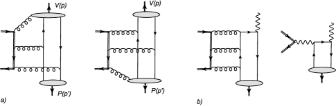
Figure 1: a) Typical diagrams describing the subprocess $Q\bar{Q}\rightarrow VP$, where $V=\rho,\gamma$. The blobs denote the light-cone matrix elements, see explanation in the text. b) An example of diagrams, describing the contribution with the perturbative photon coupling.

The long distance hadronisation dynamics of outgoing mesons is described by the twist-2 and twist-3 light-cone distribution amplitudes (LCDAs). Various properties and models for required LCDAs can be found in Refs.[7, 8]. The twist-2 light-cone matrix elements read

$$\left\langle\pi^{+}(p^{\prime})\right|\bar{u}(z_{1+})\hbox to0.0pt{\hbox to5.00002pt{\hfil$\bar{n}$\hfil}\hss}/\gamma_{5}d(z_{2+})\left|0\right\rangle=-if_{\pi}\left(p^{\prime}\bar{n}\right)\ \int_{0}^{1}du\ e^{iu\left(p^{\prime}\bar{n})(z_{1}n\right)/2+i(1-u)\left(p^{\prime}\bar{n})(z_{2}n\right)/2}\ \phi_{2\pi}(u),$$ (4)

$$\left\langle\rho^{-}(p)\right|\bar{d}(z_{1-})\gamma_{\bot}^{\mu}\hbox to0.0pt{\hbox to6.00235pt{\hfil/\hfil}\hss}nu(z_{2-})\left|0\right\rangle=if_{\rho}^{\bot}e_{\bot}^{\ast\mu}(pn)\ \int_{0}^{1}dy\ e^{iy(pn)(z_{1}\bar{n})/2+i(1-y)\left(pn)(z_{2}\bar{n}\right)/2}\ \phi_{2\rho}^{\bot}(y),$$ (5)

where we use auxiliary light-cone vectors

$$n=(1,0,0,-1),\ \bar{n}=(1,0,0,1),\ g^{\mu\nu}_{\bot}=g^{\mu\nu}-\frac{1}{2}(n^{\mu}\bar{n}^{\nu}+n^{\nu}\bar{n}^{\mu}),$$ (6)

$$p^{\prime}=(p^{\prime}\bar{n})\frac{n}{2}+\frac{m^{2}_{\pi}}{(p^{\prime}\bar{n})}\frac{\bar{n}}{2},\ p=(pn)\frac{\bar{n}}{2}+\frac{m^{2}_{\rho}}{(pn)}\frac{n}{2},\ (p^{\prime}\bar{n})\sim(pn)\sim m_{c}.$$ (7)

and the short notation for the arguments of quark fields

$$q(z_{i+})\equiv q((z_{i}n)\bar{n}/2),\ q(z_{i-})\equiv\ q((z_{i}\bar{n})n/2).$$ (8)

The required twist-3 three-particles LCDAs are defined as

$$\left\langle\pi^{+}(p^{\prime})\right|\bar{u}(z_{1+})\hbox to0.0pt{\hbox to5.00002pt{\hfil$\bar{n}$\hfil}\hss}/\gamma_{\bot}^{\mu}\gamma_{5}gG_{\bar{n}\mu}(z_{3+})d(z_{2+})\left|0\right\rangle=-2f_{3\pi}\left(p^{\prime}\bar{n}\right)^{2}\text{FT}\left[\phi_{3\pi}(u_{i})\right],$$ (9)

$$\left\langle\rho^{-}(p,e)\right|\bar{d}(z_{1-})\hbox to0.0pt{\hbox to6.00235pt{\hfil/\hfil}\hss}ngG_{\mu n}(z_{3-})u(z_{2-})\left|0\right\rangle=-\ f_{\rho}m_{\rho}(pn)^{2}e_{\bot}^{\ast\mu}\ \text{FT}\left[\phi_{3\rho}(y_{i})\right],$$ (10)

$$\left\langle\rho^{-}(p,e)\right|\bar{d}(z_{1-})\hbox to0.0pt{\hbox to6.00235pt{\hfil/\hfil}\hss}n\gamma_{5}g\tilde{G}_{\mu n}(z_{3-})u(z_{2-})\left|0\right\rangle=-if_{\rho}m_{\rho}\zeta_{3}(pn)^{2}e_{\bot}^{\ast\mu}\ \text{FT}\left[\tilde{\phi}_{3\rho}(y_{i})\right],$$ (11)

where for the gluon field strength tensor we use short notation $G_{\mu n}=G_{\mu\nu}n^{\nu}$. The dual gluon field strength tensor is defined as $\tilde{G}_{\mu\nu}=1/2\varepsilon_{\mu\nu\rho\sigma}{G}_{\rho\sigma}$ ( the Levi-Civita tensor is defined as $\varepsilon_{0123}=1$). The symbol “FT” denotes the Fourier transformation

$$\text{FT}\left[f(u_{i})\right]=\int Du_{i}\ e^{iu_{1}\left(p^{\prime}\bar{n})(z_{1}n\right)/2+iu_{2}\left(p^{\prime}\bar{n})(z_{2}n\right)/2+iu_{3}\left(p^{\prime}\bar{n})(z_{3}n\right)/2}f(u_{1},u_{2},u_{3}),$$ (12)

with

$$Du_{i}=du_{1}du_{2}du_{3}\delta(1-u_{1}-u_{2}-u_{3}).$$ (13)

The FT$\left[\phi_{3\rho}(y_{i})\right]$ is defined analogously but with $y_{i}(pn)(z_{i}\bar{n})$ in the Fourier transformation. The normalisation constants $f_{\pi,\rho}$, $\zeta_{3},\ f_{3\pi}$ and models for various LCDAs will be discussed below.

The expression for the amplitude can be written as

$$A_{\rho\pi}=\left\langle 0\right|\chi^{{\dagger}}\boldsymbol{\sigma}\cdot\boldsymbol{\epsilon}\psi\left|\psi(n,\boldsymbol{\epsilon})\right\rangle\frac{\sqrt{2M_{\psi}}}{2E}\ \frac{1}{4\pi}\int d\Omega\ \text{Tr}\left[\Pi_{1}\hat{A}_{Q}\right],$$ (14)

where $\hat{A}_{Q}$ describes subprocess $Q\bar{Q}\rightarrow\rho\pi$ with the quark-antiquark pair in the initial state. The heavy quark projector on the triplet spin state $\Pi_{1}$ reads [19]

$$\Pi_{1}=\frac{-1}{2\sqrt{2}E(E+m)}\left(\frac{1}{2}\hbox to0.0pt{\hbox to7.80904pt{\hfil/\hfil}\hss}P+m+\hbox to0.0pt{\hbox to5.00002pt{\hfil$q$\hfil}\hss}/\right)\frac{\hbox to0.0pt{\hbox to7.80904pt{\hfil/\hfil}\hss}P+2E}{4E}\hbox to0.0pt{\hbox to5.00002pt{\hfil$\epsilon$\hfil}\hss}/\left(\frac{1}{2}\hbox to0.0pt{\hbox to7.80904pt{\hfil/\hfil}\hss}P-m-\hbox to0.0pt{\hbox to5.00002pt{\hfil$q$\hfil}\hss}/\right)\otimes\frac{\mathbf{1}}{\sqrt{N_{c}}},$$ (15)

and is normalised as

$$\text{Tr}\left[\Pi_{1}\Pi_{1}^{{\dagger}}\right]=4E^{2},$$ (16)

where $E$ is the heavy quark energy $p_{Q}=(E,\boldsymbol{q})$, $p_{\bar{Q}}=(E,-\boldsymbol{q})$ and $E=\sqrt{m_{c}^{2}+\boldsymbol{q}^{2}}$. The integration $d\Omega$ over the angles of the relative momentum $\boldsymbol{q}$ in Eq.(14) is used to get the state with $L=0$. Therefore the relevant amplitude $\hat{A}_{Q}$ is the function of relative momentum square $\boldsymbol{q}^{2}$ only, which is substituted $\boldsymbol{q}^{2}\rightarrow m_{c}^{2}\left\langle{v}^{2}\right\rangle$ in the final expression (14), various technical details concerning NRQCD matching can be found in Refs.[17, 19].

Calculation of the diagrams as in Fig.1 gives

$$A_{\rho^{-}\pi^{+}}=-\left\langle 0\right|\chi^{{\dagger}}\boldsymbol{\sigma}\cdot\boldsymbol{\epsilon}\psi\left|\psi(n,\boldsymbol{\epsilon})\right\rangle\sqrt{2M_{\psi}}\left(\pi\alpha_{s}\right)^{2}\frac{10}{27}\left(1+\frac{m_{c}}{E}\right)\frac{f_{\rho}^{\bot}~{}f_{3\pi}}{\left[4E^{2}\right]^{2}}\left(J_{\pi}+\frac{\ f_{\rho}m_{\rho}\zeta_{3}\ f_{\pi}}{f_{\rho\bot}f_{3\pi}}\ J_{\rho}\right),$$ (17)

where the dimensionless collinear convolution integrals $J_{\pi}$ and $J_{\rho}$ describe contributions with twist-3 $\pi$- and $\rho$-LCDAs, respectively. These integrals also depend on the NRQCD parameter $\left\langle{v}^{2}\right\rangle$. In the leading-order limit $\left\langle{v}^{2}\right\rangle\rightarrow 0$, $E\rightarrow m_{c}^{2}$ Eq.(17) reproduces the result from Ref.[4]

$$A_{\rho^{-}\pi^{+}}^{\text{lo}}=-\left\langle 0\right|\chi^{{\dagger}}\boldsymbol{\sigma}\cdot\boldsymbol{\epsilon}\psi\left|\psi(n,\boldsymbol{\epsilon})\right\rangle\sqrt{2M_{\psi}}\left(\pi\alpha_{s}\right)^{2}\frac{20}{27}\frac{f_{\rho}^{\bot}f_{3\pi}}{\left[4m_{c}^{2}\right]^{2}}\left(J_{\pi}^{\text{lo}}+\frac{\ f_{\rho}m_{\rho}\zeta_{3}f_{\pi}}{f_{\rho\bot}f_{3\pi}}\ J_{\rho}^{\text{lo}}\right),$$ (18)

where

$$J_{\pi}^{\text{lo}} =\int Du_{i}\ \frac{\phi_{3\pi}(u_{i})}{u_{1}u_{2}u_{3}}\int_{0}^{1}dy\ \frac{\phi_{2\rho}^{\bot}(y)}{1-y}\frac{2u_{1}}{\left(y\bar{u}_{2}+u_{2}\bar{y}\right)\left(yu_{1}+\bar{y}\bar{u}_{1}\right)},$$ (19)

$$J_{\rho}^{\text{lo}} =\int_{0}^{1}du\ \frac{\phi_{2\pi}(u)}{1-u}\int Dy_{i}\ \frac{\left(\phi_{3\rho}+\tilde{\phi}_{3\rho}\right)(y_{i})}{y_{1}y_{2}y_{3}}\frac{1}{y_{2}\bar{u}+u\bar{y}_{2}},$$ (20)

with $\bar{x}=1-x$.   The analytical expressions for the integrals $J_{\pi,\rho}$ in Eq.(17) are somewhat lengthy and presented in Appendix.

In order to estimate these integrals we use the following models of LCDAs

$$\phi_{2\rho}^{\bot}(y)=6y(1-y)\left(1+a_{2\rho}\ C_{2}^{3/2}(2y-1)\right),\$$ (21)

$$\phi_{2\pi}(u)=6u(1-u)\left(1+a_{2}^{\pi}C_{2}^{3/2}(2u-1)\right),$$ (22)

$$\phi_{3\rho}(y_{i})=360y_{1}y_{2}y_{3}^{2}(y_{1}-y_{2})\omega_{3\rho},$$ (23)

$$\tilde{\phi}_{3\rho}(y_{i})=360y_{1}y_{2}y_{3}^{2}\left(1+\frac{\tilde{\omega}_{3\rho}}{\zeta_{3}}\frac{1}{2}\left(7y_{3}-3\right)\right),$$ (24)

$$\ \ \phi_{3\pi}(u_{i})=360u_{1}u_{2}u_{3}^{2}\left(1+\omega_{3\pi}\frac{1}{2}(7\alpha_{3}-3)\right).$$ (25)

The different nonperturbative moments, which enter in the definitions (4)-(11) and (21)-(25), were estimated in Refs.[4, 7, 8]. Their values are summarised in Table 1. In the numerical estimates we fix for the factorisation scale the value $\mu=2$ GeV and use $\alpha_{s}\simeq 0.30$.

Table 1: The values of the moments, which parametrise the hadronic LCDAs. All values are given at the scale $\mu=2$ GeV. For the pion moments, the values are taken from Ref.[7], for the $\rho$-meson from Ref.[8].

$f_{\pi},$MeV	$f_{\rho}$, MeV	$f_{\rho}^{\bot}$, MeV	$a_{2\pi}$	$a_{2\rho}$	$f_{3\pi},$ GeV2	$\zeta_{3\rho}$	$\omega_{3\rho}$	$\tilde{\omega}_{3\rho}$	$\omega_{3\pi}$
$131$	$216$	$143$	$0.19$	$0.11$	$0.31\times 10^{-2}$	$0.02$	$0.09$	$-0.04$	$-1.1$

All the convolution integrals calculated with the models (21)-(25) are well defined, which confirms that collinear factorisation is also valid beyond the leading-order approximation.

As a first step of the numerical analysis let us consider the the leading-order estimate for the branching ratio of $J/\psi$. For that purpose we use the estimates for the NRQCD matrix element obtained in Ref.[18]

$$\left|\left\langle 0\right|\chi^{{\dagger}}\boldsymbol{\sigma}\cdot\boldsymbol{\epsilon}\psi\left|J/\psi\right\rangle\right|^{2}\simeq 0.440\text{ GeV}^{3}.$$ (26)

For the various masses in Eq.(18) we use $M_{\psi}=3.1\$GeV, $m_{\rho}=775\$MeV, for the pole $c$-quark mass $m_{c}=1.4\$GeV and for the total width $\Gamma_{J/\psi}=93\$KeV [1]. Then for the sum of all final states $\rho^{\pm}\pi^{\mp}$ and $\rho^{0}\pi^{0}$ we obtain

$$\text{Br}[J/\psi\rightarrow\rho\pi]_{\text{lo}}\simeq 1.0\%,$$ (27)

which is somewhat smaller then the corresponding experimental value $1.69(15)\%.$ This updated result confirm the conclusion of Ref.[4], that the LO NRQCD approximation works sufficiently well for the $J/\psi$ decay. On the other hand this approximation can not describe branching ratio $\psi^{\prime}\to\rho\pi$.

Consider now the effect provided by the relativistic corrections in Eq.(17). The one part is provided by the resummation of relativistic corrections in the factor $E=m_{c}^{2}\sqrt{1+\left\langle{v}^{2}\right\rangle}$ in Eq.(17). This effect can be understood as transition from the scale $4m_{c}^{2}$ to the scale $M_{\psi}^{2}\simeq 4m_{c}^{2}(1+\left\langle{v}^{2}\right\rangle)$. These corrections reduce the ratio $Q_{\rho\pi}$ due to the factor  $(1+\left\langle{v}^{2}\right\rangle_{J/\psi})^{2}/(1+\left\langle{v}^{2}\right\rangle_{\psi^{\prime}})^{2}\sim M_{\psi}^{4}/M_{\psi^{\prime}}^{4}\sim 0.50$. However, this can not explain the very small value $Q_{\rho\pi}$ in Eq.(1).

The second effect of the relativistic corrections is associated with the modification of the hard kernels in the convolution integrals $J_{\rho,\pi}$. Because these integrals depend on meson LCDAs, the resulting effect of the relativistic corrections is also sensitive to hadronic nonperturbative structure.

For the numerical calculation we use for $J/\psi$ the estimate from Ref.[18]

$$\left\langle{v}^{2}\right\rangle_{J/\psi}\approx 0.225,$$ (28)

and for the excite state $\psi^{\prime}$ we apply the following estimate

$$\left\langle{v}^{2}\right\rangle_{\psi^{\prime}}=\frac{M_{\psi^{\prime}}-M_{J/\psi}+E_{1}}{m_{c}}\approx 0.64,$$ (29)

where $E_{1}=\left\langle{v}^{2}\right\rangle_{J/\psi}m_{c}\simeq 315\$MeV is the binding energy for $J/\psi$. The resulting value of $\left\langle{v}^{2}\right\rangle_{\psi^{\prime}}$ is much larger than $\left\langle{v}^{2}\right\rangle_{J/\psi}$, which can have a significant numerical effect and, therefore, affect the value of $Q_{\rho\pi}$.

The given calculation of the relativistic corrections is complete at the relative order $v^{2}$ only. The resummation of higher orders $\left\langle{v}^{2}\right\rangle^{n}$ with $n>2$ describes the part of the relativistic corrections associated with the quark-antiquark wave function only [19]. We use this approximation in order to study a possible effect from higher-order contributions. Therefore, for the comparison, we present the values of the integrals in Eq.(17) obtained in the leading-order approximation $J^{\text{lo}}$ ($\left\langle{v}^{2}\right\rangle\rightarrow 0$), in the next-to-leading approximation $J^{\text{nlo}}$, which takes into account the next-to-leading correction

$$J^{\text{nlo}}=J^{\text{lo}}+\left\langle{v}^{2}\right\rangle J^{(1)},$$ (30)

and the integral $J$, which includes all powers $\left\langle{v}^{2}\right\rangle^{n}$

$$J=J^{\text{lo}}+\sum\left\langle{v}^{2}\right\rangle^{n}J^{(n)}.$$ (31)

The total integral in Eq.(17) is described by the sum of two contributions with the different LCDAs

$$J_{\rho\pi}=J_{\pi}+\frac{\ f_{\rho}m_{\rho}\zeta_{3}\ f_{\pi}}{f_{\rho\bot}f_{3\pi}}\ J_{\rho},$$ (32)

where, schematically, $J_{\pi}=\phi_{3\pi}\ast T_{\pi}\ast\phi_{2\rho}^{\bot}$ and $J_{\rho}=\phi_{3\rho}\ast T_{\rho}\ast\phi_{2\pi}+\tilde{\phi}_{3\rho}\ast\tilde{T}_{\rho}\ast\phi_{2\pi}$ (the asterisk denotes the convolution integrals, $T_{\pi,\rho}$ are the hard kernels). Using parameters from Table 1 one finds

$$\frac{\ f_{\rho}m_{\rho}\zeta_{3}\ f_{\pi}}{f_{\rho\bot}f_{3\pi}}\approx 0.99.$$ (33)

Therefore the normalisation couplings in the definitions (4)-(11) do not provide any numerical difference between the two terms in Eq.(32). The results for convolution integrals (32) are presented in Table 2

Table 2: Numerical result for the convolution integrals $J_{\rho\pi}$

	$J_{\rho\pi}^{\text{lo}}$	$J_{\rho\pi}^{\text{nlo}}/J_{\rho\pi}^{\text{lo}}$	$\ J_{\rho\pi}/J_{\rho\pi}^{\text{lo}}$
$J/\psi$	$630$	$0.53$	$0.45$
$\psi^{\prime}$	$630$	$-0.46$	$-0.65$

The effect of the relativistic corrections is negative and the values of the LO integrals are substantially reduced. Notice that neglecting the higher-order corrections in $v^{2}$ in the square of the integral, one gets in case of $J/\psi$ the strong cancellation

$$|J_{\rho\pi}^{\text{nlo}}|^{2}=(J_{\rho\pi}^{\text{lo}})^{2}(2J_{\rho\pi}^{\text{nlo}}/J_{\rho\pi}^{\text{lo}}-1)+\mathcal{O}(v^{4})\simeq 0.06(J_{\rho\pi}^{\text{lo}})^{2}.$$ (34)

Therefore we assume that it is better to take the large NLO correction exactly, i.e. do not expanding the square of the integral in powers of $v^{2}$. At the same time the numerical effect from other higher order corrections is already much smaller.

For $\psi^{\prime}\to\rho\pi$ the numerical effect is bigger because $\left\langle\boldsymbol{v}^{2}\right\rangle_{\psi^{\prime}}$ is larger. One can also see that the dominant part of the correction is also provided by the contribution of relative order $v^{2}$, which is obtained exactly in this calculation. The numerical dominance of this correction can be explained by the numerical enhancement of the corresponding convolution integrals in the same way as for the baryon decays [15].

Let us assume that the relativistic correction of order $v^{2}$ provides the dominant numerical effect for $J/\psi$ and $\psi^{\prime}$ states. Then, this allows one to suggest a possible explanation of the small $\psi^{\prime}\to\rho\pi$ width, which could explain the $\rho\pi$-puzzle.

The NRQCD description of decay amplitudes also involves the $\mathcal{O}(\alpha_{s})$ NLO QCD radiative correction, which can also provide a substantial numerical effect. Usually this contribution is considered to be of the same order as relativistic corrections of relative order $v^{2}$. In this case the total convolution integral $J_{\rho\pi}$ to the next-to-leading accuracy is given by, see Eq.(30)

$$J^{\text{nlo}}_{\rho\pi}=J^{\text{lo}}+\left\langle{v}^{2}\right\rangle J^{(1)}+\alpha_{s}I^{(1)}$$ (35)

where the integrals $J^{(1)}$ and $I^{(1)}_{\rho\pi}$ describes the NLO relativistic and radiative corrections, respectively. The integral $I^{(1)}$ for $J/\psi$ and $\psi^{\prime}$ states is the same ( remind that the different leading-order NRQCD matrix elements are taken as the overall normalisation in the Eq.(17)). Therefore, if $I^{(1)}>0$ and large enough in order to cancel the negative contribution $J^{\text{lo}}+\left\langle{v}^{2}\right\rangle J^{(1)}$ for $\psi^{\prime}$, then this naturally explains the small width for $\psi^{\prime}$. It follows from the Table 2 that the required value of the radiative correction $\alpha_{s}I^{(1)}$ must be about $50\%$ of $J_{\rho\pi}^{\text{lo}}$, which is not that unrealistic given the moderate value of the charm mass.

The positive contribution $\alpha_{s}I^{(1)}$ will simultaneously improve the description of $J/\psi\to\rho\pi$ because it will compensate for the negative effect from the relativistic correction. Such cancellation is in agreement with the observation that the leading-order description $J/\psi\to\rho\pi$ provides a qualitatively good estimate.

Taking into account the values of the integrals in Table 2 and other corrections in Eq.(17) one can conclude that relativistic corrections strongly reduce the values of the branching fractions. It is clear that resulting values do not describe the data and therefore the possible effect from the radiative corrections is very important for the further progress in the understanding of this decay. Therefore, we postpone a detailed phenomenological analysis until we have a complete next-to-leading correction.

2.2 $\psi(nS)\to\gamma\pi^{0}$ decays

The considered analysis can also be applied for other decays channels $J/\psi\to VP$. The good feature of the collinear factorisation is that the hadronic nonperturbative content is described in terms of universal process independent LCDAs. Many of these functions were already studied in the literature. Even if the hard kernels are the same the differences in the models for LCDAs can affect the numerical balance and change the value $Q_{hh^{\prime}}$.

Consider, for example, the decay of S-wave charmonia into $\gamma\pi^{0}$ final state. In this case the decay amplitude is described by the same diagrams as in Fig.1(a) but with the photon LCDAs instead of $\rho$-meson. These diagrams describe the photon as a hadron, i.e. such contributions are sensitive to the nonperturbative components of the photon wave function. Such contribution can provide a sizeable impact, see e.g. discussion in Ref.[21]. We will refer to this contribution as hadronic one.

The contribution with the perturbative photon coupling appear from the diagrams Fig.1(b) only and therefore they are suppressed by electromagnetic coupling $\alpha$, which approximately scales as $\alpha^{3}_{s}$. We will call this contribution electromagnetic. On the other hand the hadronic contribution is suppressed as $\Lambda^{2}/m^{2}_{c}$ comparing to electromagnetic one. As a result both contributions can give a comparable numerical effect.

The data for the branching fractions $\psi(nS)\to\gamma\pi$ are known [1]

$$\text{Br}[J/\psi\rightarrow\gamma\pi^{0}]=3.56(17)\times 10^{-5},\ \ \text{Br}[\psi^{\prime}\rightarrow\gamma\pi^{0}]=0.104(22)\times 10^{-5},$$ (36)

which yields

$$Q_{\gamma\pi}\simeq 0.03.$$ (37)

The width $\Gamma[J/\psi\rightarrow\gamma\pi^{0}]$ can be well estimated using data for $\Gamma[J/\psi\rightarrow\rho\pi^{0}]$ and VDM model [4]. This indirectly support the picture with the large contribution from the non-perturbative photon coupling. However, the ratio $Q_{\gamma\pi}$ is about an order of magnitude larger than $Q_{\rho\pi}$. Using the results of the previous section we can calculate the hadronic contribution explicitly and clarify the role of the relativistic corrections in this decay.

The decay amplitude $A_{\gamma\pi}$ is defined similar to $A_{\rho\pi}$ in Eq.(2) with the photon instead of $\rho$-meson. Now it is given by the sum of two terms

$$A_{\gamma\pi}=A_{em}+A_{h},$$ (38)

which describe electromagnetic and hadronic contributions, respectively.

The leading-order electromagnetic contribution have been obtained in Ref.[4]. The relativistic corrections to this amplitude is similar to one in $J/\psi\to e^{+}e^{-}$, see e.g. Refs. [17, 18]. The final result reads

$$A_{em}=\left\langle 0\right|\chi^{{\dagger}}\boldsymbol{\sigma}\cdot\boldsymbol{\epsilon}\psi\left|\psi(n,\boldsymbol{\epsilon})\right\rangle\sqrt{2M_{\psi}}\frac{f_{\pi}}{M_{\psi}^{2}}\ e(4\pi\alpha)\ \frac{\sqrt{2}}{9}\ (1-f(\left\langle v^{2}\right\rangle))\int_{0}^{1}du\frac{\phi_{2\pi}(u)}{u},$$ (39)

where

$$f(x)=\frac{1}{3}\frac{x}{(1+x+\sqrt{1+x})}=\frac{x}{6}+\mathcal{O}(x^{2}).$$ (40)

The leading-order approximation is defined taking $\langle v^{2}\rangle=0$ in Eq.(39). In this limit $f(\langle v^{2}\rangle)=0$ but we leave unexpanded the quarkonium mass $M_{\psi}$, which appears in Eq.(39) from the virtual photon propagator and relativistic normalisation.

In order to compute the hadronic amplitude $A_{h}$ we use the photon LCDAs from Ref.[21]. The twist-2 light-cone matrix element is defined as

$$\left\langle\gamma(q,e)\right|\bar{q}(z_{1-})\hbox to0.0pt{\hbox to5.00002pt{\hfil$\bar{n}$\hfil}\hss}/\gamma_{\bot}^{\mu}q(z_{2-})\left|0\right\rangle=e_{q}ef_{\gamma}\varepsilon_{\bot}^{\ast\mu}(qn)\ \int_{0}^{1}dy\ e^{iy(pn)(z_{1}\bar{n})/2+i(1-y)\left(pn)(z_{2}\bar{n}\right)/2}\ \phi_{2\gamma}^{\bot}(y),$$ (41)

where $e_{u}=2/3$, $e_{d}=-1/3$, electric charge $e=\sqrt{4\pi\alpha}$. The model for $\phi_{2\gamma}^{\bot}$ reads [21]

$$\phi_{2\gamma}^{\bot}(y)\simeq 6y(1-y),\ \ \ \ f_{\gamma}(2\text{ GeV})\simeq-47\ \text{MeV}.$$ (42)

Twist-3 DAs matrix elements are defined as

$$\left\langle\gamma(p)\right|\bar{q}(z_{1-})\hbox to0.0pt{\hbox to6.00235pt{\hfil/\hfil}\hss}ngG_{\mu n}(z_{3-})q(z_{2-})\left|0\right\rangle=ie_{q}ef_{3\gamma}(qn)^{2}\varepsilon_{\bot}^{\ast\mu}\ \text{FT}\left[\phi_{3\gamma}(y_{i})\right],$$ (43)

$$\left\langle\gamma(p)\right|q(z_{1-})\hbox to0.0pt{\hbox to6.00235pt{\hfil/\hfil}\hss}n\gamma_{5}g\tilde{G}_{\mu n}(z_{2-})q(z_{3-})\left|0\right\rangle=-e_{q}ef_{3\gamma}(qn)^{2}\varepsilon_{\bot}^{\ast\mu}\ \text{FT}\left[\tilde{\phi}_{3\gamma}(y_{i})\right],$$ (44)

where Fourier transformation is the same as in Eq.(12). The corresponding models for $\phi_{3\gamma}$ and $\tilde{\phi}_{3\gamma}$ was considered in Ref.[21]

$$\phi_{3\gamma}(y_{i})=360y_{1}y_{2}y_{3}^{2}\left(y_{1}-y_{2}\right)\ \omega_{3\gamma},\ \$$ (45)

$$\tilde{\phi}_{3\gamma}(y_{i})=360y_{1}y_{2}y_{3}^{2}\left(1+\tilde{\omega}_{3\gamma}\frac{1}{2}\left(7y_{3}-3\right)\right),\ \ \tilde{\omega}_{3\gamma}\approx\tilde{\omega}_{3\rho}/\zeta_{3}.$$ (46)

where

$$f_{3\gamma}(2\text{GeV})=-0.32\times 10^{-2}\text{GeV}^{2},\ \ \omega_{3\gamma}\approx\omega_{3\rho},\ \ \ \ \tilde{\omega}_{3\gamma}\approx\tilde{\omega}_{3\rho}/\zeta_{3}.$$ (47)

The $\gamma\pi$-decay amplitude can be obtained from Eq.(17) substituting photon LCDAs instead of $\rho$-meson ones

$$A_{h}=-\left\langle 0\right|\chi^{{\dagger}}\boldsymbol{\sigma}\cdot\boldsymbol{\epsilon}\psi\left|\psi(n,\boldsymbol{\epsilon})\right\rangle\sqrt{2M_{\psi}}\left(\pi\alpha_{s}\right)^{2}\frac{10}{27}\left(1+\frac{m}{E}\right)\frac{f_{\gamma}^{\bot}f_{3\pi}}{\left[4E^{2}\right]^{2}}\left(J_{\pi}+\frac{f_{3\gamma}\ f_{\pi}}{f_{3\pi}f_{\gamma}}\ J_{\gamma}\right),$$ (48)

where, remind, $E=m_{c}\sqrt{1+\langle v^{2}\rangle}$.

The ratio of the normalisation couplings in Eq.(48) yields ($\mu=2\$GeV)

$$\frac{\ f_{3\gamma}\ f_{\pi}}{f_{3\pi}f_{\gamma}}\approx 2.92,$$ (49)

which is different from the analogous ratio for the $\rho$-meson (33).

To study the effect of the relativistic corrections we again consider three different approximations: leading-order contribution, next-to-leading order contribution (LO + the first correction), and the sum of all powers relativistic corrections as we did for the integrals in Table 2. The results for the total convolution hadronic integrals

$$J_{\gamma\pi}=J_{\pi}+\frac{f_{3\gamma}\ f_{\pi}}{f_{3\pi}f_{\gamma}}J_{\gamma},$$ (50)

are presented in Table 3.

Table 3: Numerical result for the convolution integrals $J_{\gamma\pi}$

	$J_{\gamma\pi}^{\text{lo}}$	$\ J_{\gamma\pi}^{\text{nlo}}/J_{\gamma\pi}^{\text{lo}}$	$J_{\gamma\pi}/J_{\gamma\pi}^{\text{lo}}$
$J/\psi$	$932$	$0.62$	$0.45$
$\psi^{\prime}$	$932$	$-0.49$	$-0.74$

Comparing with the analogous results for the $\rho\pi$-channel one finds that the both descriptions are qualitatively similar despite the different ratio (49) and the differences between the LCDAs $\phi_{2\gamma}$ and $\phi_{2\rho}^{\bot}$. Comparing the different relativistic corrections, one again concludes that the largest numerical effect is provided by the contribution of relative order $v^{2}$. However, in the present case, the hadronic contribution gives only a part of the overall result.

It is also useful to compare the contributions of the different amplitudes in Eq.(38) for different charmonium states. In the following numerical estimates we calculate the NRQCD matrix element for excited state $\psi^{\prime}$ in Eq.(48) using $|R_{20}(0)|^{2}=0.583\$GeV³ obtained for the Buchmüller-Tye potential in Ref.[22]. For the NLO approximation we perform expansion of the integrals $J_{\pi,\gamma}$ and the factor $(1+m/E)$ in Eq.(48) but we do not expand the factor $\left[4E^{2}\right]^{2}=[4m_{c}(1+\left\langle v^{2}\right\rangle)]^{2}$ in the denominator. This factor is closely associated with the virtualities of the gluon propagators in the diagram in Fig.1(a) and we assume that the quarkonium mass $M_{\psi}^{2}\simeq 4m_{c}^{2}(1+\left\langle{v}^{2}\right\rangle)$ is a more natural scale in this case similar to the photon virtuality in the amplitude $A_{em}$.

Table 4: Numerical result for the amplitudes $A_{em}$ and $A_{h}$ for various approximations, see more explanations in the text. The amplitudes have dimension of mass by definition, see Eq.(2), and their values are presented in MeV.

	$A_{em}[J/\psi\rightarrow\gamma\pi^{0}]$	$A_{h}[J/\psi\rightarrow\gamma\pi^{0}]$	$A_{em}[\psi^{\prime}\rightarrow\gamma\pi^{0}]$	$A_{h}[\psi^{\prime}\rightarrow\gamma\pi^{0}]$
LO	$0.351$	$0.514$	$0.205$	$+0.425$
NLO	$0.338$	$0.201$	$0.183$	$-0.065$
Sum	$0.340$	$0.147$	$0.190$	$-0.105$

These results show that relativistic corrections to $A_{em}$ are relatively small, but to $A_{h}$ they are large. For excited state they are so large that change the sign of the hadronic amplitude. As a result, the total amplitude for the $\psi\to\gamma\pi$ is much smaller compared to $J/\psi\to\gamma\pi$.

The presence of the relatively large and positive amplitude $A_{em}$ makes less critical the dependence on the numerical effect from the radiative corrections therefore it is interesting to study, at least qualitatively, the resulting values of the branching fractions. The numerical results for the different approximations are presented in the Table 5. In order to get these values we used the total widths $\Gamma_{J/\psi}=93\$KeV and $\Gamma_{\psi^{\prime}}=299$KeV from Ref.[1].

Table 5: Numerical results for the branching ratios for various approximations. The values of the branchings fractions are given in units $10^{-5}$.

	Br$[J/\psi\rightarrow\gamma\pi^{0}]$	Br$[\psi^{\prime}\rightarrow\gamma\pi^{0}]$	$Q_{\gamma\pi}$
LO	$10.83$	$1.50$	$0.138$
NLO	$4.21$	$0.05$	$0.012$
Sum	$3.43$	$0.03$	$0.008$

We observe that the LO approximation overestimates the values of the width, but relativistic corrections reduces these values by 2-3 times for $J/\psi$ and by two orders of magnitude for $\psi^{\prime}$. Therefore resulting values for $J/\psi$ are in relatively good agreement with the data while the values for $\psi^{\prime}$ are by factor 2-3 smaller. But one has to remember that we have in the background uncalculated radiative corrections and various uncertainties: unknown higher order relativistic corrections, the choice of normalisation, charm mass, meson LCDAs, etc. We postpone the detailed analysis until the radiative corrections are available. But let us notice that the strong cancellations in the amplitude for the excited state $\psi^{\prime}$ require a very precise calculation of each term to get a reliable accuracy for the difference. At the same time the hadronic amplitude has many uncertainties associated with various sources: relatively large higher order relativistic corrections, the choice of normalisation, charm mass, meson LCDAs , etc. Therefore it seems, that theoretical predictions for $\psi^{\prime}$ will have very large errors because of these uncertainties.

3 Conclusions

In conclusion, we calculated and investigated relativistic corrections to the decay amplitudes $\psi(nS)\to\rho\pi$ and $\psi(nS)\to\gamma\pi$ within the pQCD (NRQCD and collinear factorisation) framework. This calculation includes the exact correction of relative order $v^{2}$ and subset of the higher order corrections associated with the quark-antiquarks wave function. Numerical estimates show that an order $v^{2}$ correction is large and give the dominant numerical effect, which can be related to the structure of the collinear integrals. If this observation is not affected by other higher order relativistic corrections, then one has to consider the relative $v^{2}$-contribution as a special case. The obtained relativistic corrections are negative and large. In case $\psi^{\prime}\to\rho\pi$ the relative $v^{2}$ contribution is much larger than the leading-order one. Different relativistic correction effects for $J/\psi\to\rho\pi$ and $\psi^{\prime}\to\rho\pi$ suggest a scenario that may shed light on the $\rho\pi$-puzzle.

If the QCD radiative correction is positive and large enough, then it will interfere destructively with the relativistic correction for $\psi^{\prime}\to\rho\pi$, giving a small branching fraction. At the same time such radiative correction will improve the description of $J/\psi\to\rho\pi$ reducing the negative effect of the relativistic correction. Therefore, we believe that further investigation of relative order $v^{4}$ corrections and QCD radiative corrections can help to verify such a scenario.

The same approach can also be used for an analysis other similar decay channels. As a simplest example, the decay $\psi(nS)\to\gamma\pi$ is considered. In this case a part of the amplitude is given by similar diagrams but with nonperturbative photon instead of $\rho$-meson. Despite the difference between the models for the twist-2 LCDAs, the qualitative effect from the relativistic corrections is quite similar, they are also large and negative. In this case the part of the decay amplitude is described by the electromagnetic subprocess $\psi\to\gamma^{*}\to\gamma\pi$. The inclusion of the relativistic corrections allows to improve the leading-order description. Again, the large cancellation between the hadronic and electromagnetic contributions for the $\psi^{\prime}\to\gamma\pi$ leads to the small branching fraction comparing to $J/\psi\to\gamma\pi$. The obtained results show a qualitative agreement with the data. A calculation of the radiative corrections can also improve the theoretical description in this case too.

4 Appendix

Here we provide the analytical expressions for the integrals $J_{\pi}$ and $J_{\rho}$ introduced in Eq.(17). In order to simplify notations we use

$$\left\langle v^{2}\right\rangle\equiv\boldsymbol{v}^{2},\ \ \delta=1-1/\sqrt{1+\boldsymbol{v}^{2}}.\$$ (51)

The first integral in Eq.(17) reads

$$J_{\pi}\left(\boldsymbol{v}^{2}\right)=\int Du_{i}\ \frac{\phi_{3\pi}(u_{i})}{u_{1}u_{2}u_{3}}\int_{0}^{1}dy\ \frac{\phi_{2}^{\bot}(y)}{y\bar{y}}\left(\frac{2A_{\pi}}{D_{1}D_{3}}+\frac{B_{\pi}}{D_{1}D_{2}}\right),\ \ \bar{y}=1-y,$$ (52)

where

$$D_{i}=\delta_{i1}\ \left(y_{1}\bar{u}_{2}+\bar{y}_{1}u_{2}\right)+\delta_{i2}\ \left(y_{2}\bar{u}_{1}+\bar{y}_{2}u_{1}\right)+\delta_{i3}\ u_{3},$$ (53)

with

$$y_{1}=y,\ y_{2}=\bar{y}.$$ (54)

The symbol $\delta_{ik}$ denotes the Kronecker delta.

The numerators $A_{\pi}$ and $B_{\pi}~{}$are given by the sums

$$A_{\pi}=\sum_{k=0}^{4}f_{k}^{A}I_{k}[13],\ \ \ B_{\pi}=\sum_{k=0}^{4}f_{k}^{B}I_{k}[12],$$ (55)

where

$$I_{k}[ij]=\frac{1}{2}\int_{-1}^{1}d\eta\ \frac{\boldsymbol{v}^{k}\eta^{k}}{\left(1+\boldsymbol{v}\eta\ a_{i}\right)\left(1-\boldsymbol{v}\eta\ a_{j}\right)}=\frac{\boldsymbol{v}^{k}}{a_{i}+a_{j}}\sum_{n=0}^{\infty}\boldsymbol{v}^{n}\frac{a_{j}^{n+1}+(-1)^{n}a_{i}^{n+1}}{n+1+k}\frac{1}{2}\left[1+(-1)^{n+k}\right].\ \$$ (56)

with

$$a_{j}=\delta_{1j}\left(1-\delta\right)\frac{y_{1}-u_{2}}{y_{1}\bar{u}_{2}+\bar{y}_{1}u_{2}}+\delta_{2j}\left(1-\delta\right)\frac{y_{2}-u_{1}}{y_{2}\bar{u}_{1}+\bar{y}_{2}u_{1}}-\delta_{3j}\left(1-\delta\right).$$ (57)

The coefficients $f_{k}^{A,B}\equiv f_{k}^{A,B}(u_{i},y;\delta)$ in Eq.(55) read

$$f_{0}^{A}=\frac{\delta}{2}\left(3u_{3}-2-\delta\right),\ \ \ \ f_{1}^{A}=\frac{\delta}{2}\frac{\left(1-\delta\right)}{\left(2-\delta\right)}u_{3},$$ (58)

$$f_{2}^{A}=\frac{1}{2}\frac{\left(1-\delta\right)^{2}}{\left(2-\delta\right)^{2}}\left(4-3(2-\delta)u_{3}+2\delta(1-\delta)\right),$$ (59)

$$f_{3}^{A}=-\frac{1}{2}\frac{\left(1-\delta\right)^{3}}{\left(2-\delta\right)^{2}}u_{3},\ \ f_{4}^{A}=-\frac{1}{2}\frac{\left(1-\delta\right)^{4}}{\left(2-\delta\right)^{2}}.$$ (60)

$$f_{0}^{B} =u_{1}y_{1}+u_{1}y_{2}-\frac{\delta}{2}(u_{1}+u_{2}+y_{1}+y_{2}-\delta)$$ (61)

$$+\frac{\delta}{2-\delta}\left(u_{1}y_{1}+u_{1}y_{2}-(2-\delta)\left(u_{1}+u_{2}+y_{1}+y_{2}\right)+(2-\delta)^{2}\right),$$ (62)

$$f_{1}^{B}=\frac{1}{2}\frac{\left(1-\delta\right)}{\left(2-\delta\right)}\left\{4(u_{1}y_{1}-u_{2}y_{2})+\delta(u_{1}+y_{1}-u_{2}-y_{2})\right\},$$ (63)

$$f_{2}^{B} =\frac{1}{2}\frac{\left(1-\delta\right)^{2}}{\left(2-\delta\right)^{2}}\left\{6\left(u_{1}+u_{2}+y_{1}+y_{2}\right)-2\left(u_{1}y_{1}+u_{1}y_{2}\right)-8\right.$$ (64)

$$\left.+\delta\left(4-3\left(u_{1}+u_{2}+y_{1}+y_{2}\right)\right)+2\delta(2-\delta)\right\},$$ (65)

$$f_{3}^{B}=-\frac{1}{2}\frac{\left(1-\delta\right)^{3}}{\left(2-\delta\right)^{2}}\left(u_{1}+y_{1}-u_{2}-y_{2}\right),\ \ f_{4}^{B}=-\frac{1}{2}\frac{\left(1-\delta\right)^{4}}{\left(2-\delta\right)^{2}}.$$ (66)

The $\rho$-meson integral in Eq.(17) reads

$$J_{\rho}=\int_{0}^{1}du\ \frac{\phi_{2\pi}(u)}{u\bar{u}}\int Dy_{i}\ \ \frac{1}{y_{1}y_{2}y_{3}}\left(\frac{2A_{\rho}}{y_{3}D_{2}}+\frac{B_{\rho}}{D_{1}D_{2}}\right).$$ (67)

The numerators $A_{\rho}$ and $B_{\rho}$ can be written as

$$A_{\rho}=\phi_{3\rho}(y_{i})\sum_{k=0}^{4}\left[f_{k}^{A}\right]I_{k}[23]+\tilde{\phi}_{3\rho}(y_{i})\sum_{k=0}^{4}\left[\tilde{f}_{k}^{A}\right]I_{k}[23],$$ (68)

$$B_{\rho}=\phi_{3\rho}(y_{i})\sum_{k=0}^{4}\left[f_{k}^{B}\right]I_{k}[12]+\tilde{\phi}_{3\rho}(y_{i})\sum_{k=0}^{4}\left[\tilde{f}_{k}^{B}\right]I_{k}[12],$$ (69)

where the integrals $I_{k}$ are defined in Eq.(56) with a bit different combination $a_{j}$

$$a_{j}=\delta_{1j}\left(1-\delta\right)\frac{y_{1}-u_{2}}{y_{1}\bar{u}_{2}+\bar{y}_{1}u_{2}}+\delta_{2j}\left(1-\delta\right)\frac{y_{2}-u_{1}}{y_{2}\bar{u}_{1}+\bar{y}_{2}u_{1}}+\delta_{3j}\left(1-\delta\right)\ ,$$ (70)

and we again use for the two-particle LCDA $\ u_{1}=u$, $u_{2}=1-u$.

The coefficients $f_{k}^{A,B}$ and $\tilde{f}_{k}^{A,B}$ defined in Eqs.(68) and (69) read

$$f_{0}^{A} =\frac{1}{4}\left(u_{1}(2y_{3}-\delta)+\delta\left(\delta-y_{2}-y_{3}\right)\right)+\frac{\delta^{2}}{2}$$ (71)

$$\ \ \ \ \ \ \ \ \ \ +\frac{1}{4}\frac{\delta}{(2-\delta)}\left(u_{1}\left(6+4y_{3}-3\delta\right)+\left(2-\delta\right)\left(3y_{2}+2y_{3}-2-3\delta\right)\right),$$ (72)

$$f_{1}^{A} =-\frac{1}{4}\frac{1-\delta}{2-\delta}\left(4u_{1}+\delta\right)y_{3},$$ (73)

$$f_{2}^{A}=-\frac{1}{4}\frac{(1-\delta)^{2}}{(2-\delta)^{2}}\left(2u_{1}y_{3}+(2-\delta)\left(2u_{1}+2y_{2}+y_{3}\right)-2(1-\delta)(2-\delta)\right),$$ (74)

$$f_{3}^{A}=\frac{1}{4}\frac{(1-\delta)^{3}}{(2-\delta)^{2}}y_{3},\ \ f_{4}^{A}=0.$$ (75)

$$f_{0}^{B} =-f_{2}^{B}=\frac{\delta}{4}\left(u_{1}-u_{2}-y_{1}+y_{2}\right),\$$ (76)

$$\ \ f_{1}^{B} =-f_{3}^{B}=-\frac{\delta}{4}(1-\delta)\left(u_{1}+u_{2}-y_{1}-y_{2}\right),\ \ \ f_{4}^{B}=0.$$ (77)

$$\tilde{f}_{0}^{A} =\frac{1}{4}\left(u_{1}(2y_{3}-\delta)+\delta\left(\delta-y_{2}-y_{3}\right)\right)$$ (78)

$$+\frac{1}{4}\frac{\delta}{(2-\delta)}\left(u_{1}\left(2+4y_{3}-\delta\right)+\left(2-\delta\right)\left(2+y_{2}-2y_{3}-3\delta\right)\right),$$ (79)

$$\tilde{f}_{1}^{A}=-\frac{1}{4}\frac{1-\delta}{2-\delta}\left(4u_{1}y_{3}+\delta\left(2u_{1}-2y_{2}+y_{3}\right)\right),$$ (80)

$$\tilde{f}_{2}^{A}=-\frac{1}{4}\frac{(1-\delta)^{2}}{(2-\delta)^{2}}\left(2u_{1}y_{3}-3y_{3}(2-\delta)+\delta(2-\delta)\right),$$ (81)

$$\tilde{f}_{3}^{A}=\frac{1}{4}\frac{(1-\delta)^{3}}{(2-\delta)^{2}}\left(2u_{1}-2y_{2}+y_{3}\right),\ \ \ \tilde{f}_{4}^{A}=-\frac{1}{2}\frac{(1-\delta)^{4}}{(2-\delta)^{2}}.$$ (82)

$$\tilde{f}_{0}^{B}=\frac{\delta}{4}\left(3\left(u_{1}+u_{2}+y_{1}+y_{2}\right)-4-2\delta\right),\ \ \ \tilde{f}_{1}^{B}=-\frac{\delta}{4}\frac{1-\delta}{2-\delta}\left(u_{1}-u_{2}+y_{1}-y_{2}\right),$$ (83)

$$\tilde{f}_{2}^{B}=\frac{1}{4}\frac{(1-\delta)^{2}}{(2-\delta)^{2}}\left(8-3\left(2-\delta\right)\left(u_{1}+u_{2}+y_{1}+y_{2}\right)+4\delta(1-\delta)\right),$$ (84)

$$\tilde{f}_{3}^{B}=\frac{1}{4}\frac{(1-\delta)^{3}}{(2-\delta)^{2}}\left(u_{1}-u_{2}+y_{1}-y_{2}\right),\ \ \ \tilde{f}_{4}^{B}=-\frac{1}{2}\frac{(1-\delta)^{4}}{(2-\delta)^{2}}.$$ (85)

References

• [1] R. L. Workman et al. [Particle Data Group], PTEP 2022 (2022), 083C01
• [2] N. Brambilla et al. [Quarkonium Working Group], hep-ph/0412158.
• [3] X. H. Mo, C. Z. Yuan and P. Wang, Chin. Phys. C 31 (2007), 686-701 [arXiv:hep-ph/0611214 [hep-ph]].
• [4] V. L. Chernyak and A. R. Zhitnitsky, Phys. Rept. 112 (1984) 173.
• [5] A. R. Zhitnitsky, I. R. Zhitnitsky and V. L. Chernyak, Yad. Fiz. 41 (1985), 199-208
• [6] P. Ball and V. M. Braun, [arXiv:hep-ph/9808229 [hep-ph]].
• [7] P. Ball, V. M. Braun and A. Lenz, JHEP 05 (2006), 004 [arXiv:hep-ph/0603063 [hep-ph]].
• [8] P. Ball and G. W. Jones, JHEP 03 (2007), 069 [arXiv:hep-ph/0702100 [hep-ph]].
• [9] V. Chernyak, [arXiv:hep-ph/9906387 [hep-ph]].
• [10] Y. Q. Chen and E. Braaten, Phys. Rev. Lett. 80 (1998), 5060-5063 [arXiv:hep-ph/9801226 [hep-ph]].
• [11] M. Suzuki, Phys. Rev. D 63 (2001), 054021 [arXiv:hep-ph/0006296 [hep-ph]].
• [12] J. L. Rosner, Phys. Rev. D 64 (2001), 094002 [arXiv:hep-ph/0105327 [hep-ph]].
• [13] G. T. Bodwin, E. Braaten and G. P. Lepage, Phys. Rev. D 51 (1995) 1125 [Phys. Rev. D 55 (1997) 5853] [hep-ph/9407339].
• [14] E. Braaten and J. Lee, Phys. Rev. D 67 (2003), 054007 [erratum: Phys. Rev. D 72 (2005), 099901] [arXiv:hep-ph/0211085 [hep-ph]].
• [15] N. Kivel, “A study of relativistic corrections to $J/\psi\rightarrow p\bar{p}$ decay,” [arXiv:2211.13603 [hep-ph]].
• [16] J. H. Kuhn, J. Kaplan and E. G. O. Safiani, Nucl. Phys. B 157 (1979), 125-144
• [17] G. T. Bodwin and A. Petrelli, Phys. Rev. D 66 (2002), 094011 [erratum: Phys. Rev. D 87 (2013) no.3, 039902] [arXiv:hep-ph/0205210 [hep-ph]].
• [18] G. T. Bodwin, H. S. Chung, D. Kang, J. Lee and C. Yu, Phys. Rev. D 77 (2008), 094017 [arXiv:0710.0994 [hep-ph]].
• [19] G. T. Bodwin, J. Lee and C. Yu, Phys. Rev. D 77 (2008), 094018 [arXiv:0710.0995 [hep-ph]].
• [20] G. T. Bodwin, D. Kang and J. Lee, Phys. Rev. D 74 (2006), 014014 doi:10.1103/PhysRevD.74.014014 [arXiv:hep-ph/0603186 [hep-ph]].
• [21] P. Ball, V. M. Braun and N. Kivel, Nucl. Phys. B 649 (2003), 263-296 [arXiv:hep-ph/0207307 [hep-ph]].
• [22] E. J. Eichten and C. Quigg, Phys. Rev. D 52 (1995), 1726-1728 doi:10.1103/PhysRevD.52.1726 [arXiv:hep-ph/9503356 [hep-ph]].