Sigma terms of the baryon octet in $N_{\mathrm{f}}=2+1$ QCD
with Wilson quarks

Abstract

A lot of progress has been made in the direct determination of nucleon sigma terms. Using similar methods, we consider the sigma terms of the other octet baryons as well. These are determined on CLS gauge field ensembles employing the Lüscher-Weisz gluon action and the Sheikholeslami-Wohlert fermion action with $N_{\mathrm{f}}=2+1$. The ensembles have pion masses ranging from ${410}\,\mathrm{MeV}$ down to the physical value and lattice spacings covering a range between ${0.098}\,\mathrm{fm}$ and ${0.039}\,\mathrm{fm}$. We present some preliminary results for the pion and strange sigma terms and compare to indirect determinations. To do so, we discuss multi-state fits to tackle the well-known problem of excited state contamination comparing the ratio and summation methods also including priors.

1 Introduction

The sigma terms encode the quark contributions to the mass of a baryon. They are defined as the matrix element of a scalar current $J$ times the quark mass such that

$$\sigma_{qB}=m_{q}\langle B|J|B\rangle\,,$$ (1)

where $J=\bar{q}\,\mathds{1}\,q$ and the quark flavour $q\in\{u,d,s\}$. In order to compare with phenomenological determinations, the pion-baryon sigma terms are usually constructed, $\sigma_{\pi B}=\sigma_{uB}+\sigma_{dB}$. In the matrix element, $B$ refers to the ground state of a baryon $B$. Of particular interest are the nucleon sigma terms ($B=N$) which appear in the expressions for WIMP-nucleon scattering cross-sections and are relevant for comparing model predictions to the exclusion bounds obtained from direct detection dark matter experiments (such as the XENON1T experiment).

In the analysis, we make use of and adjust methods established for the nucleon (see ref. [1] for a review). We determine the sigma terms of the baryon octet, i.e. of the lambda $\Lambda$, sigma $\Sigma$ and cascade $\Xi$ baryons. This enables us to investigate SU(3) flavour symmetry breaking and to determine the SU(3) low energy constants (LECs), that are currently not well known. There have been relatively few determinations so far, see, for example, refs. [2] and [3], with most previous studies focusing on the nucleon sigma terms (see ref. [4] for a review).

In addition, discrepancies between results for the pion-nucleon sigma term from Lattice QCD and phenomenology are still to be resolved (see [4], and e.g., [5, 6, 7]). In a recent paper, results more consistent with phenomenology were obtained by explicitly including $N\pi$ and $N\pi\pi$ excited states in the analysis [8, 9]. By considering baryons other than the nucleon, we aim to understand excited state contributions and other issues in more detail so as to help solve this puzzle.

2 Excited state analysis

In order to be able to extract the ground-state matrix element, we need to take care of the excited state contamination. Two possible approaches are the ratio method and the summation method (reviewed in [10, 1]) that are both based on spectral decompositions. We consider the two- and three-point functions of a baryon (from the octet) at rest in the initial and final state. The spectral decomposition of the two-point function reads

$$C_{\mathrm{2pt}}({t_{\mathrm{f}}})=\sum_{\vec{x}}\left\langle\mathcal{O}_{\mathrm{snk}}(\vec{x},{t_{\mathrm{f}}})\bar{\mathcal{O}}_{\mathrm{src}}(\vec{0},0)\right\rangle=\sum_{n}|Z_{n}|^{2}e^{-E_{n}{t_{\mathrm{f}}}}\,,$$ (2)

where $Z_{n}\propto\langle\Omega|\mathcal{O}_{\mathrm{snk}}|n\rangle$ is the overlap of the interpolator $\mathcal{O}_{\mathrm{snk}}$ onto the state $n$ (and $\Omega$ the vacuum state) and ${t_{\mathrm{f}}}$ the source-sink separation. Summation over spin and colour indices and projection onto positive parity are implied. These indices become apparent when writing down the operators explicitly. The interpolators for the four octet baryons are set to

$$\mathcal{O}_{\mathrm{snk}}^{\alpha,\mathrm{N}} =\epsilon^{abc}u_{a}^{\alpha}\left(u_{b}^{\beta}(C\gamma_{5})^{\beta\gamma}d_{c}^{\gamma}\right)\quad\text{and}\quad\mathcal{O}_{\mathrm{snk}}^{\alpha,\Lambda}=\epsilon^{abc}s_{a}^{\alpha}\left(u_{b}^{\beta}(C\gamma_{5})^{\beta\gamma}d_{c}^{\gamma}\right),$$

$$\mathcal{O}_{\mathrm{snk}}^{\alpha,\Sigma} =\epsilon^{abc}u_{a}^{\alpha}\left(u_{b}^{\beta}(C\gamma_{5})^{\beta\gamma}s_{c}^{\gamma}\right)\quad\,\text{and}\quad\mathcal{O}_{\mathrm{snk}}^{\alpha,\Xi}=\epsilon^{abc}s_{a}^{\alpha}\left(s_{b}^{\beta}(C\gamma_{5})^{\beta\gamma}u_{c}^{\gamma}\right).$$ (3)

$a,b,c$ are colour indices, $\alpha,\beta,\gamma$ are spin indices and $\mathcal{O}_{\mathrm{src}}^{\alpha}=\mathcal{O}_{\mathrm{snk}}^{\alpha}$ and $\bar{\mathcal{O}}_{\mathrm{src}}=\mathcal{O}_{\mathrm{src}}^{\dagger}\gamma_{4}$. $C$ stands for the charge conjugation operator. Note that for the $\Lambda$ we use a naive interpolator that also has overlap with the (heavier) $\Sigma^{0}$. Turning to the three-point function, its spectral decomposition reads

$$C_{\mathrm{3pt}}({t_{\mathrm{f}}},t) =\sum_{\vec{x},\vec{y}}\left\langle\mathcal{O}_{\mathrm{snk}}(\vec{x},{t_{\mathrm{f}}})J(\vec{y},t)\bar{\mathcal{O}}_{\mathrm{src}}(\vec{0},0)\right\rangle-\sum_{\vec{x},\vec{y}}\left\langle J(\vec{y},t)\right\rangle\left\langle\mathcal{O}_{\mathrm{snk}}(\vec{x},{t_{\mathrm{f}}})\bar{\mathcal{O}}_{\mathrm{src}}(\vec{0},0)\right\rangle$$

$$=\sum_{n,n^{\prime}}Z_{n^{\prime}}Z_{n}^{*}\langle n^{\prime}|J|n\rangle e^{-E_{n}t}e^{-E_{n^{\prime}}({t_{\mathrm{f}}}-t)},$$ (4)

where $t$ is the insertion time of the scalar current, $J=\bar{q}\,\mathds{1}\,q$. As $J$ has the same quantum numbers as the vacuum, the vacuum expectation value needs to be subtracted, see the second term in the first line of eq. (4). Note that depending on the type of baryon and current, different Wick contractions (e.g. different currents) contribute that result in connected and disconnected quark-line diagrams.
Ratio method:
Taking the ratio of the two spectral decompositions and truncating after the first excited state contribution leads to

$$R({t_{\mathrm{f}}},t)=\frac{C_{\mathrm{3pt}}({t_{\mathrm{f}}},t)}{C_{\mathrm{2pt}}({t_{\mathrm{f}}})}=g_{S}^{q}+c_{01}\mathrm{e}^{-\Delta\,\cdot\,t}+c_{10}\mathrm{e}^{-\Delta\,\cdot\,({t_{\mathrm{f}}}-t)}+c_{11}\mathrm{e}^{-\Delta\,\cdot\,{t_{\mathrm{f}}}}+...$$ (5)

where $g_{S}^{q}=\langle B|\bar{q}\,\mathds{1}\,q|B\rangle$ is the ground-state matrix element of interest. $\Delta=E_{1}-E_{0}$ is the energy gap between the ground and first excited state. The coefficients $c_{01}$, $c_{10}$, $c_{11}$ are made up of matrix elements for different transitions, $B_{0}\rightarrow B_{1}$, $B_{1}\rightarrow B_{0}$ , and $B_{1}\rightarrow B_{1}$, respectively. Here, $B_{0}$ refers to the ground state of the baryon while $B_{1}$ denotes the first excited state (single- or multi-particle state). As the baryon is at rest, $c_{01}=c_{10}\equiv c_{0\leftrightarrow 1}$. Note that we labelled $c_{0\leftrightarrow 1}$ as $c_{1}$ in [11].
Summation method:
Summing over the ratio (5) for a range of insertion times leads to

$$\sum_{t/a=c}^{{\small t_{\mathrm{f}}/a-c}}R(t_{\mathrm{f}},t)=g_{S}^{q}(t_{\mathrm{f}}/a-2c+1)+\frac{2c_{0\leftrightarrow 1}}{1-\mathrm{e}^{a\Delta}}\left(\mathrm{e}^{\Delta(c-t_{\mathrm{f}})}-\mathrm{e}^{\Delta(a-c)}\right)+c_{11}({\small t_{\mathrm{f}}/a}-2c+1)\mathrm{e}^{-\Delta\,\cdot\,t_{\mathrm{f}}}+{\small...}$$ (6)

where $a$ refers to the lattice spacing and $c>0$ to preserve reflection positivity (we set $c=2$). An advantage of this method is that, in principle, the slope, $\frac{\mathrm{d}\quad\,}{\mathrm{d}(t_{\mathrm{f}}/a)}\sum_{t/a=c}^{t_{\mathrm{f}}/a-c}R(t_{\mathrm{f}},t)=g_{S}^{q}+\mathrm{O}(t_{\mathrm{f}}/a\,\cdot\,\mathrm{e}^{-\Delta\,\cdot\,t_{\mathrm{f}}})\,,$ approaches the asymptotic value faster compared to the ratio method. However, a large number of source-sink separations is required and due to the the numerical setup we use (discussed in the next section) we can only employ this approach for the disconnected three-point functions.

3 Numerical Setup

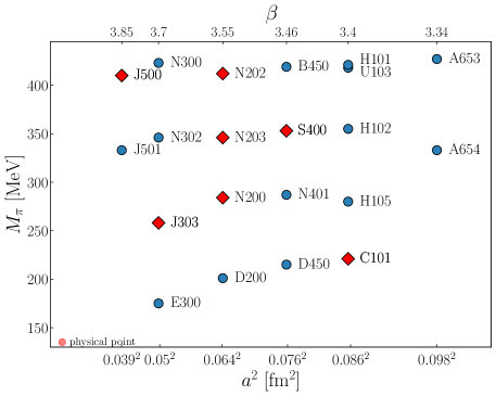
Figure 1: Overview of a subset of the CLS ensembles which lie on a trajectory which starts at a symmetric point ($m_{l}=m_{s}$, $M_{\pi}\sim 410$ MeV) and extends to the physical point, along which the flavour average of the quark masses is held constant. So far the ensembles highlighted in red (diamonds) have been analysed.

We utilise the CLS gauge field ensembles [12], which are generated employing the Lüscher-Weisz gluon action and the Sheikholeslami-Wohlert fermion action with $N_{\mathrm{f}}=2+1$ ($m_{l}=m_{u}=m_{d}\leq m_{s}$). The pion-baryon and strange sigma terms are determined on the seven ensembles highlighted in red (diamonds) in fig. 1. This includes five lattice spacings in the range from $a=0.08528(49)$ fm down to $a=0.03875(22)$ fm. The pion masses vary from 411 MeV down to 222 MeV, see also [13] .

To compute the connected three-point correlation functions on the ensembles with $m_{l}=m_{s}$ and $M_{\pi}=410$ MeV, we used the standard sequential source method [15]. On the other ensembles we employed the stochastic method described in [16, 17] (see also [18, 19, 20, 21]). This approach enables us to obtain measurements for all baryons of interest at multiple source and insertion positions, simultaneously. Four different source-sink separations, corresponding to ${t_{\mathrm{f}}}\approx[0.71\,\mathrm{fm},0.9\,\mathrm{fm},1.03\,\mathrm{fm},1.22\,\mathrm{fm}]$, are employed. Two measurements are performed for each ${t_{\mathrm{f}}}$ on every configuration except for the $m_{l}=m_{s}$ ensembles (that we used the sequential source method for) where ten measurements are typically performed (one, two, three and four measurements for ${t_{\mathrm{f}}}\approx[0.71\,\mathrm{fm},0.9\,\mathrm{fm},1.03\,\mathrm{fm},1.22\,\mathrm{fm}]$, respectively).

The disconnected three-point functions are constructed by correlating a quark loop with a baryon two-point function. The loop is estimated stochastically on every timeslice (within the bulk) leading to additional noise on top of the Monte-Carlo gauge sampling. In order to reduce the noise, the truncated solver method [22], the hopping parameter expansion technique [23] and time partitioning [24] are utilised. Between twenty and thirty measurements of the two-point functions (at different temporal source positions) are performed on each configuration. A reasonable signal for the disconnected three-point function is obtained for a source-sink separation of up to ${t_{\mathrm{f}}}\approx 1.22\,\mathrm{fm}$. For the analysis of the statistical errors we employ the $\Gamma$-method [25] (that is based on autocorrelation functions) using the pyerrors python package [26].

When constructing the sigma terms for Wilson-type fermions, one needs to take the mixing between different quark flavours into account, which arises due to the singlet and non-singlet combinations of the scalar current renormalising differently as a result of chiral symmetry breaking (see , e.g., [11] for the renormalisation pattern). For the ratio of renormalisation factors, $r_{\mathrm{m}}$, we use $r_{\mathrm{m}}(\beta=3.4)=2.335(31)$, $r_{\mathrm{m}}(\beta=3.46)=1.869(19)$, $r_{\mathrm{m}}(\beta=3.55)=1.523(14)$, $r_{\mathrm{m}}(\beta=3.7)=1.267(16)$ and $r_{\mathrm{m}}(\beta=3.85)=1.149(18)(27)[33]$, determined non-perturbatively in [27].

4 Fitting Analysis

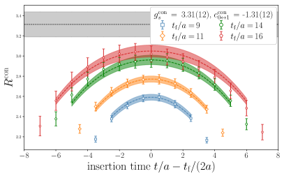
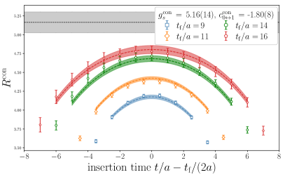
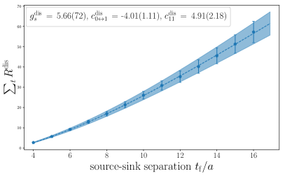
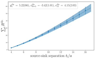
Figure 2: The connected and (summed) disconnected ratios contributing to the unrenormalised scalar charges of the $\Xi$ baryon on ensemble S400 ($M_{\pi}\approx 350$ MeV) for the $\bar{u}u$ current (left) and the $\bar{s}s$ current (right): Simultaneous fits to the connected and summed disconnected ratios are indicated by the coloured shaded regions. The resulting connected ground state scalar matrix elements are displayed as horizontal grey bands.

In order to extract the ground-state matrix elements of interest while taking the excited state contamination into account we perform multi-state fits, applying the ratio method, eq. (5) and, for comparison, for the disconnected contribution also the summation method, eq. (6) (as noted in sect. 2, there are not enough source-sink separations available to apply this method to the connected contributions). For each baryon, we fit the connected and disconnected ratios for all currents simultaneously, with the energy gap to the first excited state $\Delta$ as the common fit parameter. As an example, the ratios (and fits) relevant for determining the sigma terms of the $\Xi$ baryon on the S400 ensemble ($M_{\pi}\approx 350$ MeV) are displayed in fig. 2 (see fig. 2 in [11] for an example of the ratio method being used for both the connected and disconnected contributions). While we were able to resolve the first excited state term, with the coefficient $c_{0\leftrightarrow 1}$, with both methods, the $B_{1}\to B_{1}$ transition term (see sect. 2) was not resolved when employing the ratio method and we set $c_{11}=0$ in the analysis when using this method. The $\chi^{2}/\chi_{\mathrm{expected}}^{2}$ were mostly below 1.5 (and always below two), where $\chi_{\mathrm{expected}}^{2}$ provides an estimate of the effective degrees of freedom expected taking into account autocorrelations, see [28].

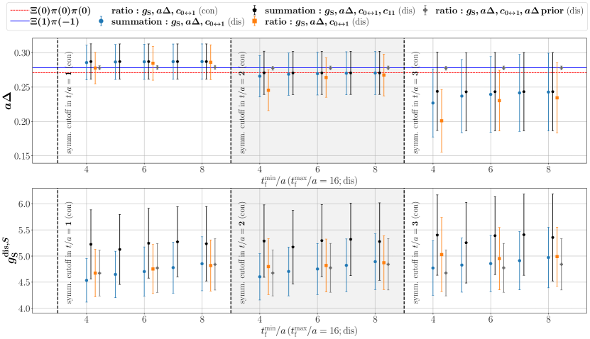
Figure 3: Effect of the fit form and range variation on the energy gap $\Delta=E_{1}-E_{0}$ (top) and the disconnected scalar charge $g_{S}^{\mathrm{dis}}$ for $J=\bar{s}s$ (bottom) for the $\Xi$ baryon on the ensemble S400 ($M_{\pi}\approx 350$ MeV). The blue and red-dashed horizontal lines indicate an energy gap corresponding to a $\Xi(1)\pi(-1)$ and $\Xi(0)\pi(0)\pi(0)$ excited state, respectively. The numbers in brackets stand for the momentum as a multiple of the lowest lattice momentum $2\pi/L$. Each of the three panels displays results of simultaneous fits to the connnected and disconnected contributions where the fit range is fixed for the former and varied for the latter, while across the different panels, the fit range for the connected ratio is varied. The insertion times included are always symmetric w.r.t. the source and sink. This leads to a minimal ${t_{\mathrm{f}}}$ for the fits to the disconnected ratios (for which all ${t_{\mathrm{f}}}$ are, in principle, available). For the connected contributions only the ratio method (with $c_{11}=0$) is employed, while for the disconnected results both the ratio and the summation method are shown. Results for the ratio method, using a prior (Gaussian with $\sigma=1\%$) for the energy gap corresponding to a $\Xi(1)\pi(-1)$ (non-interacting) excited state, are also displayed. The first (black) pentagon corresponds to the fit in fig. 2.

To investigate whether the excited state contributions are sufficiently controlled when extracting the ground state matrix elements, we vary the fit range for both the connected and disconnected contributions and for the latter also the fit method. In addition, we consider the impact on the fit of a narrow-width prior for $\Delta$. The fit range is varied by removing insertion times symmetrically for each source-sink separation. The results for the example of S400 are displayed in fig. 3. We find that the energy gap is mostly determined by the connected data: in the first row of fig. 3 the error on $\Delta$ increases as more connected data points are excluded from the fit. We also observe that the energy gap $\Delta=E_{1}-E_{0}$ is compatible with that for a ${\Xi(1)\pi(-1)}$ or $\Xi(0)\pi(0)\pi(0)$ first excited state so that a narrow-width prior corresponding to a ${\Xi(1)\pi(-1)}$ excited state has almost no effect on the ground-state matrix elements (second row of fig. 3). This is also true for the other members of the baryon octet (when comparing to the energy of a ${B(1)\pi(-1)}$ or $B(0)\pi(0)\pi(0)$ excited state). However, as the pion mass decreases, with the exception of the nucleon, we find $E_{1}$ to be larger than the energies of these levels. This may be related to the fact that the spectrum (for the nucleon) is denser at smaller pion masses [10] making it more difficult to separate the first excited state contributions from others. However, we can enforce the first excitation to have the energy of a non-interacting $B(1)\pi(-1)$ state by using a narrow-width prior and the sigma terms are usually only mildly affected, see fig. 4.

5 Preliminary results and consistency with indirect determinations

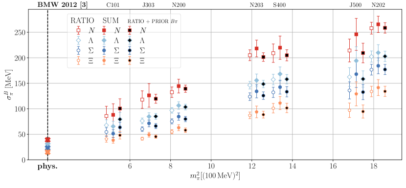
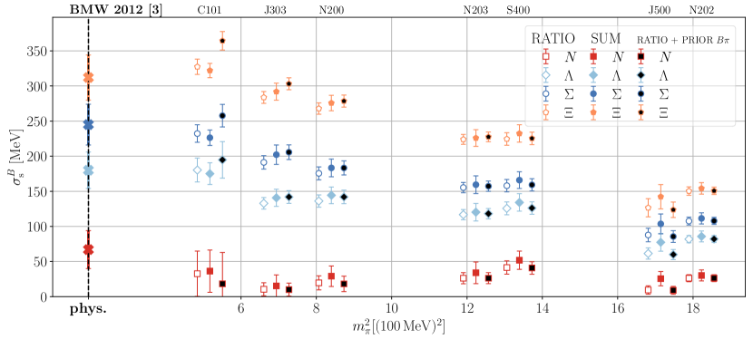
Figure 4: Preliminary results for the pion-baryon and strange sigma terms as a function of the pion mass squared obtained utilising the ratio method (with $c_{11}=0$) for both contributions (with and without a prior for the energy gap) and utilising the ratio method for the connected contribution and the summation method (with $c_{11}\neq 0$) for the disconnected contribution. The prior width is set to $1\%$ centered around an energy gap compatible with a ${B(1)\pi(-1)}$ excited state. We also compare our results to those of BMW 2012 [3].

The ground-state matrix elements of interest are extracted from the fits presented in the previous section and combined with the corresponding quark masses and renormalisation factors (see [11]) to form the pion-baryon and strange sigma terms for all four octet baryons. Our preliminary results are displayed as a function of the pion mass squared in fig. 4. We see that the different fitting methods employed lead to compatible results for the sigma terms. In addition, we compare our results from the ratio method (extracted at finite lattice spacing) in fig. 5 to the quark mass dependence in the continuum limit obtained from an indirect determination via the Feyman-Hellmann theorem and a fit to the octet baryon masses, see [13]. Almost all our preliminary results (from our direct determination) lie within the error bands of the indirect determination suggesting that, after having taken the continuum and infinite volume limits, the results will remain consistent.

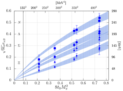
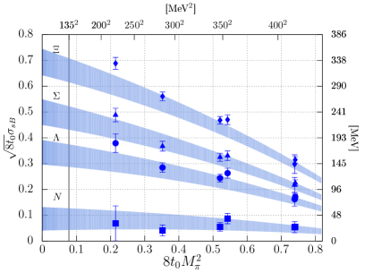
Figure 5: Results for the pion-baryon and strange sigma terms as a function of the pion mass squared obtained using the ratio method (blue squares). The shaded regions show the quark mass dependence of $\sigma_{\pi}^{B}$ and $\sigma_{s}^{B}$ determined via the Feynman-Hellmann theorem utilising a fit to the octet baryon masses evaluated on 47 CLS ensembles [13]. Finite-volume effects are accounted for and NNLO baryon chiral perturbation theory is used to describe the quark mass dependence.

6 Conclusion and outlook

Our aim is to determine the strange and pion sigma terms for the baryon octet. In these proceedings we reported on the progress made in controlling excited state contaminations. We find that the ratio and summation methods give compatible results for the sigma terms. Although these methods do not always result in a first excited state compatible with a ${B(1)\pi(-1)}$ or $B(0)\pi(0)\pi(0)$ state (for octet baryons other than the nucleon), when a narrow-width prior is used for the energy gap, consistent results for the sigma terms are, nonetheless, obtained. The next steps will include analysing additional ensembles so as to allow for an extrapolation to the physical point and an investigation of cut-off and finite-volume effects.

References

- [1] K. Ottnad, Excited states in nucleon structure calculations, Eur. Phys. J. A 57 (2021) 50 [2011.12471].
- [2] P. E. Shanahan et al., Sigma terms from an SU(3) chiral extrapolation, Phys. Rev. D 87 (2013) 074503 [1205.5365].
- [3] S. Dürr et al., Sigma term and strangeness content of octet baryons, Phys. Rev. D 85 (2012) 014509 [1109.4265], [Erratum: Phys.Rev.D 93, 039905 (2016)].
- [4] Flavour Lattice Averaging Group (FLAG) collaboration, Y. Aoki et al., FLAG Review 2021, Eur. Phys. J. C 82 (2022) 869 [2111.09849].
- [5] C. Alexandrou et al., Nucleon axial, tensor, and scalar charges and -terms in lattice QCD, Phys. Rev. D 102 (2020) 054517 [1909.00485].
- [6] S. Borsanyi et al., Ab-initio calculation of the proton and the neutron’s scalar couplings for new physics searches, 2007.03319.
- [7] M. Hoferichter et al., Remarks on the pion–nucleon -term, Phys. Lett. B 760 (2016) 74 [1602.07688].
- [8] R. Gupta et al., Pion–Nucleon Sigma Term from Lattice QCD, Phys. Rev. Lett. 127 (2021) 242002 [2105.12095].
- [9] R. Gupta et al., The pion-nucleon sigma term from Lattice QCD, in 10th International workshop on Chiral Dynamics, 3, 2022, 2203.13862.
- [10] J. Green, Systematics in nucleon matrix element calculations, PoS LATTICE2018 (2018) 016 [1812.10574].
- [11] P. L. J. Petrak et al., Towards the determination of sigma terms for the baryon octet on CLS ensembles, PoS LATTICE2021 (2022) 072 [2112.00586].
- [12] M. Bruno et al., Simulation of QCD with flavors of non-perturbatively improved Wilson fermions, JHEP 02 (2015) 043 [1411.3982].
- [13] RQCD collaboration, G. S. Bali et al., Scale setting and the light baryon spectrum in QCD with Wilson fermions, 2211.03744.
- [14] RQCD collaboration, G. S. Bali et al., Leading order mesonic and baryonic SU(3) low energy constants from lattice QCD, Phys. Rev. D 105 (2022) 054516 [2201.05591].
- [15] L. Maiani et al., Scalar Densities and Baryon Mass Differences in Lattice QCD With Wilson Fermions, Nucl. Phys. B 293 (1987) 420.
- [16] G. S. Bali et al., Hyperon couplings from lattice QCD, PoS LATTICE2019 (2019) 099 [1907.13454].
- [17] G. S. Bali et al., Baryonic and mesonic 3-point functions with open spin indices, EPJ Web Conf. 175 (2018) 06014 [1711.02384].
- [18] Y.-B. Yang et al., Stochastic method with low mode substitution for nucleon isovector matrix elements, Phys. Rev. D 93 (2016) 034503 [1509.04616].
- [19] ETM collaboration, C. Alexandrou et al., A Stochastic Method for Computing Hadronic Matrix Elements, Eur. Phys. J. C 74 (2014) 2692 [1302.2608].
- [20] G. S. Bali et al., Nucleon structure from stochastic estimators, PoS LATTICE2013 (2014) 271 [1311.1718].
- [21] R. Evans et al., Improved Semileptonic Form Factor Calculations in Lattice QCD, Phys. Rev. D 82 (2010) 094501 [1008.3293].
- [22] G. S. Bali et al., Effective noise reduction techniques for disconnected loops in Lattice QCD, Comput. Phys. Commun. 181 (2010) 1570 [0910.3970].
- [23] C. Thron et al., Pade - Z(2) estimator of determinants, Phys. Rev. D 57 (1998) 1642 [hep-lat/9707001].
- [24] S. Bernardson et al., Monte Carlo methods for estimating linear combinations of inverse matrix entries in lattice QCD, Comput. Phys. Commun. 78 (1993) 256.
- [25] U. Wolff, Monte Carlo errors with less errors, Comput. Phys. Commun. 156 (2004) 143 [hep-lat/0306017], [Erratum: Comput. Phys. Commun. 176, 383 (2007)].
- [26] F. Joswig et al., pyerrors: a python framework for error analysis of Monte Carlo data, 2209.14371.
- [27] J. Heitger, et al., Ratio of flavour non-singlet and singlet scalar density renormalisation parameters in QCD with Wilson quarks, Eur. Phys. J. C 81 (2021) 606 [2101.10969].
- [28] M. Bruno et al., On fits to correlated and auto-correlated data, 2209.14188.
- [29] Jülich Supercomputing Centre, JURECA: Modular supercomputer at Jülich Supercomputing Centre, Journal of large-scale research facilities 4 (2018) .
- [30] Jülich Supercomputing Centre, HDF Cloud – Helmholtz Data Federation Cloud Resources at Jülich Supercomputing Centre, Journal of large-scale research facilities 5 (2019) .