WKB Across Caustics: The Screened-WKB Method

Abstract

We present a new methodology, based on the WKB approximation and Fast Fourier Transforms, for the evaluation of wave propagation through inhomogeneous media. This method can accurately resolve fields containing caustics, while still enjoying the computational advantages of the WKB approximation, namely, the ability to resolve arbitrarily high-frequency problems in computing times which are orders-of-magnitude shorter than those required by other algorithms presently available. For example, the proposed approach can simulate with high accuracy (with errors such as e.g. 0.1%–0.001%) the propagation of 5 cm radar signals across two-dimensional configurations resembling atmospheric ducting conditions, spanning hundreds of kilometers and millions of wavelengths in electrical size, in computing times of a few minutes in a single CPU core. [Preliminary version]

1 Introduction

Computations of high-frequency wave propagation through inhomogeneous media play a pivotal roles in diverse fields such as telecommunications, remote sensing, seismics, quantum mechanics, and optics. A wide range of methodologies have been developed over the last century for the treatment of high-frequency volumetric-propagation problems. Given that direct numerical simulation of the configurations of interest, which comprise thousands to millions of wavelengths in acoustical/electrical size, is unfeasible in 2D and even more in 3D, the proposed approaches usually contain a combination of analytic and numerical approximations.

The celebrated WKB approximation, also known as the Wentzel-Kramers-Brillouin approximation [2, 8], was the first method to obtain accurate solutions to problems involving propagation over large distances, and is based on the introduction of a system of ray-coordinates, over which the amplitude and phase of the solution exhibit slow variations. However, the WKB approximation can break down in certain situations, particularly when the ray mapping becomes singular (i.e. at caustics). Many approaches have been proposed over time to overcome this limitation, most notably the KMAH-index theory, according to which a correction can be incorporated after the caustic, of the form $(-i)^{m}$, where the constant $m$ depends on the number and type of caustics that the ray has traversed. This formulation still breaks down at caustics, is inaccurate near caustics, and, given its complexity, it is seldom used in practice.

Another notable approach to solve these type of problems is provided by the parabolic approximation introduced in [9], together with its many subsequent versions and improvements, including the wide-angle approximation [5]. The method of phase-screens [14], in turn, which assumes a constant refractivity profile along each vertical volumetric screen, is applicable for certain restricted sets of configurations. While, unlike the classical WKB approach, these methods are valid at and around caustics, their limitations arise from its computational cost. For example, mesh-sizes of the order of $\Delta z\approx\frac{\lambda}{4}$ and $\Delta x\approx 12.5\lambda$ are reported for propagation distances in the order of a few hundreds of wavelengths (see [7] and references therein). (Here $z$ and $x$ denote the vertical and range variables, respectively.) The parabolic equation methods are most often based on use of finite-difference approximations, which gives rise to associated dispersion errors, while Fourier expansions in the vertical axis are only applicable in the lowest-order parabolic approximations. The combined effect of large propagation distances, and the presence of dispersion error, and the requirement of fine spatial discretizations, can lead to extremely large computational cost, under reasonable error tolerances, for challenging configurations commonly arising in applications.

Other notable approaches include the Gaussian beams formulation, with contributions spanning from the 60’s, including [1, 3, 13, 6] among many others. This formulation is based on an additional approximation to WKB, which seeks to obtain the phase in the form of a quadratic polynomial, whose Hessian matrix is evolved along the ray. This approach eliminates ray-bunching at caustics, and produces fields which remain bounded. However, theoretical convergence as $k\to\infty$ has not been established and is believed to be slow. Moreover, the initial beam representation is a challenging optimization problem, which leads to errors of a few percent even for propagations distances of the order of a small number of wavelengths [13].

An additional approach, known as Dynamic Surface Extension (DSE, see [12, 11]), can successfully propagate wavefronts in a Cartesian discretization. However, the amplitude computations present the same limitations as the classical WKB approximation. Finally, the Kinetic Formulation [4] views each ray tracing equation as describing the motion of a ”particle” (e.g. photon, phonon). This method presents severe computational difficulties, as the initial conditions and solutions are given in terms of Wigner measures, a $\delta$-function that vanishes for incorrect directions $p$.

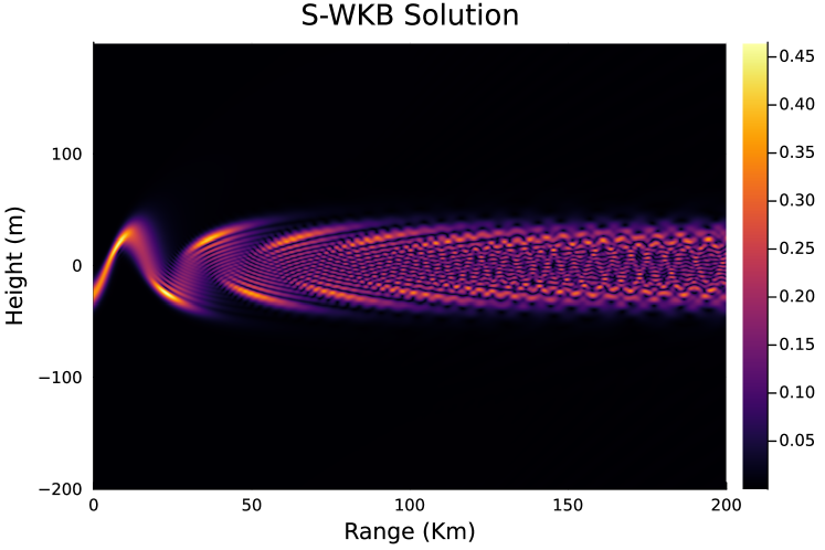
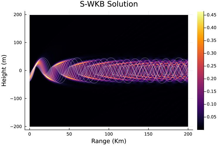
Figure 6: “Multiple caustics” test case depicting an idealized “ducting” configuration. S-WKB field values (top), and field values with super-imposed geometrical-optics rays (bottom). The geometrical optics rays are depicted in Figure 5.

The approach put forth in this paper, on the other hand, is based on the WKB approximation, and overcomes the limitations posed by caustics by resorting to a family of curves (or screens) on which the total field is decomposed in Fourier modes. Each mode is then propagated for large electrical distances (i.e. 20,000$\lambda$ in the example considered in Figure 6) which are also short enough that the presence of caustics is avoided for each Fourier mode.

2 The Screened WKB Method

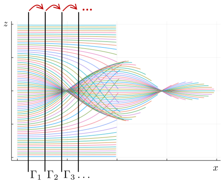
Figure 1: Schematics underlying the proposed S-WKB method. Here and throughout this paper flat screens $\Gamma_{q}$ are used, but curved screens could alternatively be utilized, if convenient.

We consider, as a model problem, the scalar Helmholtz equation

$$\Delta u(\mathbf{r})+k^{2}\varepsilon(\mathbf{r})u(\mathbf{r})=0$$ (1)

$$u=u^{s}+u^{\mathrm{inc}}$$ (2)

$$\lim_{r\to\infty}r\left(\frac{\partial u^{s}}{\partial r}-iku^{s}\right)=0,$$ (3)

whose character at high frequencies presents challenges often found in diverse fields, such high-frequency electromagnetism, acoustics, seismics and quantum mechanics. The proposed screened-WKB approach first introduces a family of curves (or screens) $\Gamma_{q}$, for $q=0,1,\dots,N_{s}$, as depicted in Figure 1. The method proceeds by propagating the solution from one screen to the next on the basis of Fourier expansions on the screens $\Gamma_{q}$ and applications of the classical WKB approach for each separate Fourier mode.

For conciseness, we consider planar screens of the form $\Gamma_{q}=\{(x_{q},z):z\in(z_{a},z_{b})\}$. The initial conditions on $\Gamma_{0}$ are user-prescribed, and given by:

$$u|_{\Gamma_{0}}=u^{\mathrm{inc}}|_{\Gamma_{0}}$$ (4)

We then represent the incident field on each screen $\Gamma_{q}$, arising from propagation of the field from $\Gamma_{q-1}$ (or given by (4) for $q=0$) by exploiting certain expressions of the form

$$u(x,z)\approx\sum_{n=-N/2}^{N/2-1}A^{q}_{n}(x,z)\exp(ik\psi^{q}_{n}(x,z)),$$ (5)

valid between $\Gamma_{q}$ and $\Gamma_{q+1}$, together with the WKB approximation.

For simplicity, in our description we consider configurations which may accurately be expressed in terms of $z$-periodic functions, of period $[z_{a},z_{b}]$, which, in particular, can be used to treat cases wherein the solution decays rapidly outside a bounded interval in the $z$ variable. (Other arrangements, including rough top and bottom surfaces and other irregularities, can also be incorporated in this framework, but are not considered in this paper at any length.) Under such assumptions, for a given screen $\Gamma_{q}$, a “vertical” DFT can be used by introducing an equi-spaced grid

$$\{z_{m}\,:\,m=-N/2,\dots,N/2-1\}$$ (6)

in the interval $[z_{a},z_{b}]$ and performing an FFT—which yields

$$w^{q}_{j}=\sum_{m=-N/2}^{N/2-1}u(x_{q},z_{m})e^{-ijz_{m}}.$$ (7)

Then, re-expressing the field $u(x_{q},z)$ in terms of an inverse DFT, we obtain

$$u|_{\Gamma_{q}}\approx\frac{1}{N}\sum_{m=-N/2}^{N/2-1}w^{q}_{j}e^{ijz_{m}},$$ (8)

which may be expressed in terms of (5) by requiring that

$$\psi^{q}_{n}(x_{q},z)=\left(z+\frac{z_{b}-z_{a}}{2}\right)\frac{2n\pi}{k(z_{b}-z_{a})}.$$ (9)

As a second step, each term in the expansion (5) is obtained up to the next screen $\Gamma_{q+1}$ by means of the classical WKB expansion (see e.g. [7, chapter 3]), which, in particular, requires the solution of the Eikonal and Transport equations

$$(\nabla\psi)^{2}=\varepsilon(r)$$ (10)

and

$$2\nabla\psi\cdot\nabla A+A\Delta\psi=0.$$ (11)

In the present case, the initial conditions for each Fourier mode on $\Gamma_{q}$ are obtained from (9) and (10):

$$\partial_{z}\psi_{n}(x_{q},z)=\frac{2n\pi}{k(z_{b}-z_{a})}$$ (12)

$$\partial_{x}\psi_{n}(x_{q},z)=\sqrt{\varepsilon(x_{q},z)-\left(\frac{2n\pi}{k(z_{b}-z_{a})}\right)^{2}}$$ (13)

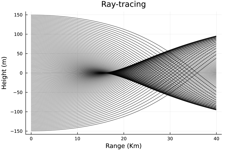
Figure 2: Example 1: Ray-tracing leading to a single cusp caustic.

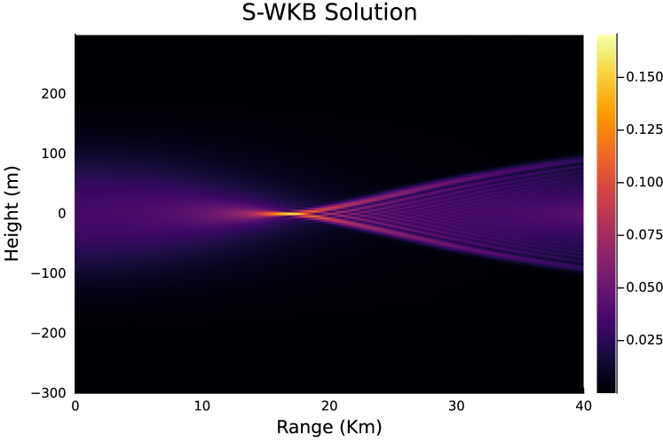
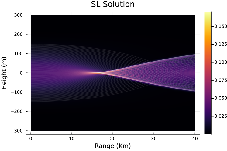
Figure 3: S-WKB solution (top), and physically-exact separation-of-variables solution with super-imposed geometrical-optics rays (bottom), with $k=125$, along a propagation domain $40$ km ($800,000$ wavelengths) in range.

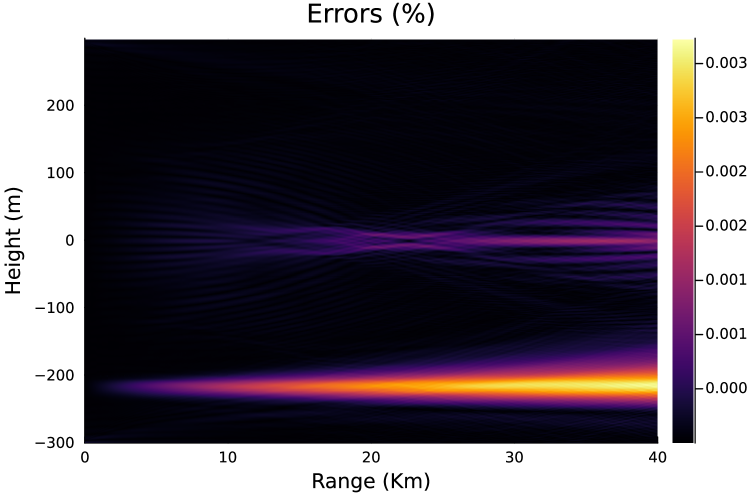
Figure 4: Error for the “single-caustic” solution displayed in Figure (3): a relative error of the order of $10^{-5}$ was obtained throughout the propagation domain.

This procedure yields a finite number of adequately spaced geometrical-optics rays, and corresponding values of $\psi_{n}$ and $A_{n}$ along the rays for the $n$-th mode. By adequately selecting the spacing of the screens $\Gamma_{q}$ it can ensured that all the modes $-\frac{N}{2}\leq n\leq\frac{N}{2}-1$ propagate to the next screen $\Gamma_{q+1}$ without incurring caustics. Interpolation can then be used on $\Gamma_{q+1}$ to obtain approximate values of $u$ on the 1D Cartesian grid $(x_{q+1},z_{m})$ ($-\frac{N}{2}\leq n\leq\frac{N}{2}-1$) on $\Gamma_{q+1}$:

$$u(x_{q+1},z_{m})\approx\sum_{n=-N/2}^{N/2-1}A^{q}_{n}(x_{q+1},z_{m})\exp(ik\psi^{q}_{n}(z_{m})).$$ (14)

Expanding $u(x_{q+1},z)$ in a Fourier series along $\Gamma_{q+1}$ the next iteration of the algorithm can then be initiated. Repeating this procedure for all screens the field $u$ over the domain of interest can be obtained.

3 Numerical Results

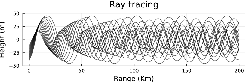
Figure 5: Geometrical optics rays for a “ducting” configuration.

This section presents results of applications of the proposed algorithm to problems of wave propagation through inhomogeneous media, in two-dimensional configurations, and through wide ranges of problem parameters. In order to evaluate the accuracy of the proposed S-WKB method by comparisons with solutions obtainable by means of separation of variables, we first consider $x$-invariant permittivities (i.e. permittivities of the form $\varepsilon(x,z)=\varepsilon(z)$), as described in what follows, for which a simple high-order spectral solver can be used to obtained reference solutions that are physically-exact—i.e., which contain no approximations to (1) other than those inherent in the well established numerical solver utilized.

3.1 High-order reference solutions for $x$-invariant permittivities

In order to obtain a valid solution to (1) via separation of variables we seek a solution of the form

$$u(x,z)=\sum_{i=0}^{\infty}a_{i}e^{i\alpha_{i}x}\phi_{i}(z).$$ (15)

Substituting (15) in (1) leads to

$$\sum_{i=0}^{\infty}(-\alpha^{2}+\phi_{i}^{\prime\prime}(z)+k^{2}\varepsilon(z))a_{i}e^{i\alpha_{i}x}=0.$$ (16)

Using the orthogonality of the complex exponentials we then obtain

$$(-\alpha_{i}^{2}+\phi_{i}^{\prime\prime}(z)+k^{2}\varepsilon(z))a_{i}=0.$$ (17)

It follows that the non-zero coefficients $\alpha_{i}$ in (15) satisfy the Sturm-Liouville problem:

$$\phi_{i}^{\prime\prime}(z)+k^{2}\varepsilon(z)\phi_{i}(z)=\alpha_{i}^{2}\phi_{i}(z)$$ (18)

with radiation boundary conditions:

$$\lim_{z\to\pm\infty}\left(z\phi_{i}^{\prime}-ik\phi_{i}\right)=0,$$ (19)

Numerically, the radiation boundary conditions can be imposed by considering a sufficiently large interval $(z_{a},z_{b})$ and imposing either Dirichlet or periodic boundary conditions at such points. The resulting Sturm-Liouville problem can be discretized with high-order spectral methods. For the purposes of the present paper we utilized the spectral eigensolver [10], which is available in the ApproxFun.jl Julia package.

3.2 Evaluation of the S-WKB accuracy for a Gaussian permittivity model

In this section we consider the exponential permittivity model

$$\varepsilon(z)=1+ae^{-bz^{2}}$$ (20)

whose physically-exact solution can be obtained by relying on the method described in Section 3.1. For our example, an incident field given by a Gaussian beam

$$u_{\mathrm{inc}}(x,z)=\int_{-\infty}^{\infty}e^{i\sqrt{k^{2}-\beta^{2}}x+i\beta z}e^{-\frac{\beta^{2}}{\sigma^{2}}}d\beta$$ (21)

is utilized, wherein the integral in the variable $\beta$ is evaluated via standard numerical integration techniques.

In our first example we consider the permittivity model (20) with parameters $a=10^{-4}$ and $b=10^{-4}$—which, at C-band, results in a configuration that gives rise to a single caustic of cusp type for the first $40$km ($800,000$ wavelengths) in horizontal propagation range. The geometrical optics rays are displayed in Fig. 2. The S-WKB solution alongside the Sturm-Liouville solution with superimposed ray-tracing are depicted in Fig. 3. As shown in Fig. 4, the relative errors for this configuration are of the order of $10^{-5}$. Employing $N=400$ Fourier modes and a total of $40$ screens, the S-WKB solution in this case was obtained in a computing times of 2 minutes in a single-core, whereas the separation-of-variables solution required single-core runs of approximately 1.5 hours.

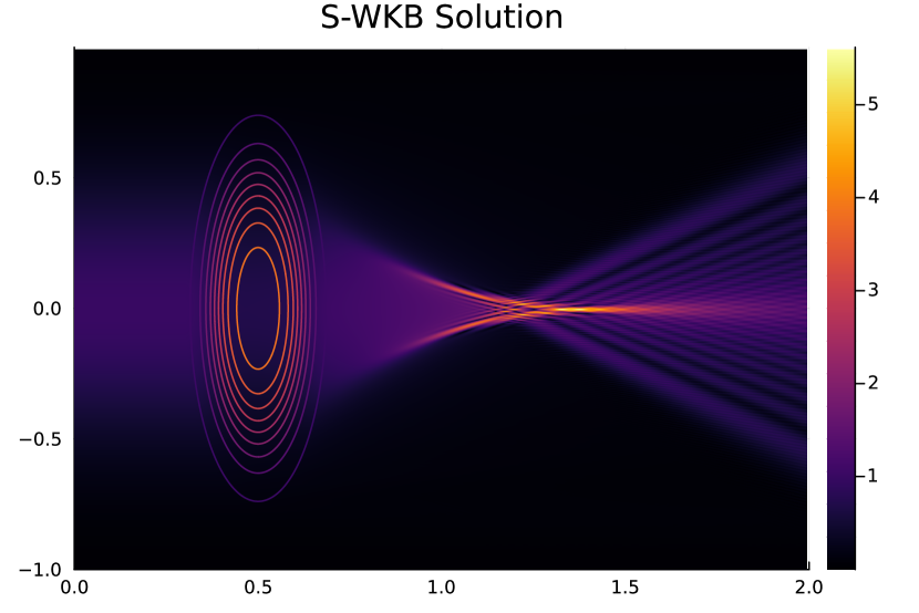
Figure 7: Smooth convex lens simulations produced by the S-WKB method. Note the fine-scale fields behind caustics, whose simulation is otherwise quite challenging; cf. e.g. [7, Fig. 6.10].

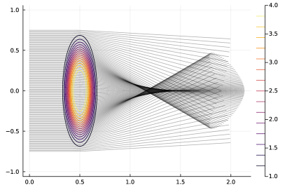
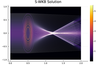
Figure 8: Permittivity and geometrical-optics rays (left), and rays superimposed on the field depicted in Figure 7.

For our next example we consider a “ducting” configuration, in which the incident Gaussian beam is tilted by an angle of $0.2^{\circ}$, and where the Gaussian permittivity (20) was used with parameters $a=10^{-4}$ and $b=10^{-3}$—in such a way that the energy is contained within a bounded interval along the $z$ axis. The geometrical-optics rays form a complex system with multiple caustics, as depicted in Fig. 5. We consider the propagation of this signal over a range of $200Km$ (4 million wavelengths) in range. A total of $n=800$ Fourier modes and $200$ of the order of $0.1\%$.

4 Smooth Lens

We now consider the test case of a smooth convex lens proposed in [4] on the basis of the permittivity function given by

$$\varepsilon(r)=\left\{\begin{array}[]{cr}1&d^{2}>L\\ \left(\frac{a}{b-\cos(\pi d^{2})}\right)^{2}&d^{2}\leq L\end{array}\right.\qquad d^{2}=\left(\frac{x-x_{c}}{x_{d}}\right)^{2}+\left(\frac{z-z_{c}}{z_{d}}\right)^{2}$$ (22)

For the numerical example depicted in Fig. 7, we have set $L=1,a=4,b=3,x_{c}=0.5,x_{d}=0.2,z_{c}=0,z_{d}=0.8$. The displayed result compares favorably to that presented in [4] on the basis of a kinetic formulation, as well as the similar problem demonstrated in [7, Fig. 6.10]. A separation of variables solution is not available in this case, and the error could be evaluated by means of S-WKB implementation of higher order. In presence of the previous examples, however, we may estimate the error in the range of $0.1\%$ to $0.001\%$.

References

- [1] Vasilii M Babich and Vladimir Sergeevich Buldyrev. Short-wavelength diffraction theory: asymptotic methods. Springer, 1991.
- [2] Max Born and Emil Wolf. Principles of optics: electromagnetic theory of propagation, interference and diffraction of light. Elsevier, 2013.
- [3] Vlastislav Červenỳ, Mikhail M Popov, and Ivan Pšenčík. Computation of wave fields in inhomogeneous media—gaussian beam approach. Geophysical Journal International, 70(1):109–128, 1982.
- [4] Björn Engquist and Olof Runborg. Computational high frequency wave propagation. Acta numerica, 12:181–266, 2003.
- [5] RH Hardin. Applications of the split-step fourier method to the numerical solution of nonlinear and variable coefficient wave equations. SIAM Review (Chronicles), 15, 1973.
- [6] Lars Hörmander. Linear partial differential operators. Springer, 1963.
- [7] Finn B Jensen, William A Kuperman, Michael B Porter, Henrik Schmidt, and Alexandra Tolstoy. Computational ocean acoustics, volume 794. Springer, 2011.
- [8] Joseph B Keller. Geometrical theory of diffraction. Josa, 52(2):116–130, 1962.
- [9] Mikhail Aleksandrovich Leontovich and Vladimir Aleksandrovich Fock. Solution of the problem of propagation of electromagnetic waves along the earth’s surface by the method of parabolic equation. J. Phys. Ussr, 10(1):13–23, 1946.
- [10] Sheehan Olver and Alex Townsend. A fast and well-conditioned spectral method. siam REVIEW, 55(3):462–489, 2013.
- [11] Steven J Ruuth, Barry Merriman, and Stanley Osher. A fixed grid method for capturing the motion of self-intersecting wavefronts and related pdes. Journal of Computational Physics, 163(1):1–21, 2000.
- [12] John Steinhoff, Meng Fan, and Lesong Wang. A new eulerian method for the computation of propagating short acoustic and electromagnetic pulses. Journal of Computational Physics, 157(2):683–706, 2000.
- [13] Nicolay M Tanushev, Björn Engquist, and Richard Tsai. Gaussian beam decomposition of high frequency wave fields. Journal of Computational Physics, 228(23):8856–8871, 2009.
- [14] Ru-Shan Wu. Wide-angle elastic wave one-way propagation in heterogeneous media and an elastic wave complex-screen method. Journal of Geophysical Research: Solid Earth, 99(B1):751–766, 1994.