Assessing the applicability of common performance metrics for real-world infrared small-target detection

Abstract

Infrared small target detection (IRSTD) is a challenging task in computer vision. During the last two decades, researchers’ efforts are devoted to improving detection ability of IRSTDs. Despite the huge improvement in designing new algorithms, lack of extensive investigation of the evaluation metrics are evident. Therefore, in this paper, a systematic approach is utilized to: First, investigate the evaluation ability of current metrics; Second, propose new evaluation metrics to address shortcoming of common metrics. To this end, after carefully reviewing the problem, the required conditions to have a successful detection are analyzed. Then, the shortcomings of current evaluation metrics which include pre-thresholding as well as post-thresholding metrics are determined. Based on the requirements of real-world systems, new metrics are proposed. Finally, the proposed metrics are used to compare and evaluate four well-known small infrared target detection algorithms. The results show that new metrics are consistent with qualitative results.

Keywords: Infrared small target detection; thresholding; pre-thresholding metrics; post-thresholding metrics

1 Introduction

Nowadays, infrared (IR) imaging has a wide range of application from medical [1, 2] and industrial diagnosis [3] to defense [4] and remote sensing [5]. Generally, processing IR images is a challenging task [6] due to the specifications of IR imaging. Among all the aforementioned applications, IR small target detection (IRSTD) is a highly challenging research field because:

• Since the IR small targets are far from the imaging device, the target has low local contrast and appears as a dim spot in the image plane [7].

• The small target in IR images typically occupies handful of pixels [8]. Thus, the region of interest (ROI) does not represent distinguished features.

• The edges of the small target are blurred due to atmospheric thermal fields [9]. Therefore, there are not a clear boundary between background area and target pixels.

The block diagram of a typical IRSTD pipeline is illustrated in Fig. 1. As shown in the figure, the input IR image is first process by the IRSTD algorithm to create a saliency map. Note that, while the IRSTD algorithm may refer to the end-to-end IR image processing pipeline, here, the process of construction of saliency map from input IR image is called IRSTD algorithm. The goal is to suppress the background area and enhance target pixels. An ideal saliency map should eliminate the background intensities and only preserve the target area. After saliency map reconstruction, a thresholding strategy is chosen to be applied on the saliency map. Then, true (logical one) pixels in the resulting binary image is considered as target-like objects.

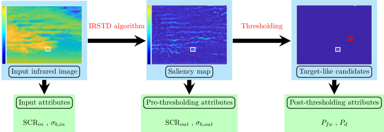
Figure 1: The block diagram of a typical IRSTD pipline

Considering the pipeline in the Fig. 1, specific attributes are defined for images in pipeline. In IRSTD terminology, the input image can be represented by two attributes:

• $\sigma_{b,in}$ which denotes the standard deviation of background pixels in input image. This parameter directly related to the background complexity. Smaller $\sigma_{b,in}$ represents smooth backgrounds, while larger $\sigma_{b,in}$ belongs to a complicated background.

• SCR_in stands for signal to clutter ratio in the input image. SCR is defined as $\frac{\mu_{t}-\mu_{b}}{\sigma_{b}}$. Where, $\mu_{t}$, $\mu_{b}$, and $\sigma_{b}$ are the mean value of target pixels, mean value of the local background pixels, and standard deviation of the local background, respectively.

Same argument is valid for saliency map (The processed image by IRSTD algorithm). Thus, just like the input attributes, $\sigma_{b,out}$ and SCR_out represents the background complexity and the signal to clutter ration in the saliency map. It is clear that for a typical IRSTD pipeline:

$$\sigma_{b,out}<\sigma_{b,in}\quad\text{and}\quad\text{SCR}_{out}>\text{SCR}_{in}$$ (1)

According to Eq. 1, two performance metrics are defined for evaluation of IRSTD algorithms: Background suppression factor (BSF) and signal to clutter ration gain (SCRG) which are defined as follows [10]:

$$\text{BSF}=\frac{\sigma_{b,in}}{\sigma_{b,out}}\quad,\quad\text{SCRG}=\frac{\text{SCR}_{out}}{\text{SCR}_{in}}$$ (2)

Based on Eq. 1 and Eq. 2, larger values for both SCRG and BSF are desired. Note that, in case of evaluation of different IRSTD algorithms, since the input images are the same for all baseline algorithms, $\text{SCR}_{out}$ and $\frac{1}{\sigma_{b,out}}$ can be used as performance metrics, as well.

The IRSTD algorithms are well-studied in the literature. Mainly, these algorithms can be categorized based on filtering method, contrast measure calculation, and data structure decomposition [11].

The filtering based methods are divided into two sub-categories. The first one is the spatial domain filtering, in which, the input infrared image is processed using local kernels to enhance the target area. Max-mean [12], max-median [12], bilateral filtering [13], morphological operators [14], two dimensional least mean square [15] are some instances of this sub-category. The second one refers to processing in the transformation domain. In these techniques, the input image is transformed to a desired transformation space like as frequency [16] and wavelet [17] domains. Then, after processing the transformed information, the inverse transform is applied to recover true targets.

Methods based on human visual systems (HVS) which lead to local contrast-based mechanism has received researchers’ attention during last few years. These methods outperform filter-based methods in terms of SCRG and BSF. However, they usually have higher computational complexity compared to filter-based ones. Generally, local contrast can be constructed in either difference or ratio forms. Difference local contrast like as Laplacian of Gaussian (LoG) [18], difference of Gaussian (DoG) [19], improved difference of Gabor [20], center-surround difference measure [21], and local difference adaptive measure [22]. Unlike the difference form local measures, ratio-form local measures utilize enhancement factor which is the ration between the center cell and surrounding ones. Local contrast measure (LCM) [23], improved local contrast measure (ILCM) [24], relative local contrast measure (RLCM) [25], Tri-Layer local constrast method (TLLCM) [26], novel local contrast descriptor (NLCD) [27], and weighted strengthened local contrast measure (WSLCM) [28] are the most effective IRSTDs in the literature. There is also a combined local measure which benefits from both difference and ratio from of local contrast measure [29].

Data structure decomposition-based methods are also a newly introduced class of IRSTDs. Sparse and low-rank matrices decomposition is the principal of these class of IRSTDs. Infrared patch image (IPI) model [30], weighted infrared patch image (WIPI) model [31], non-negative infrared patch image model based on partial sum minimization of singular values (NIPPS) [32], nonconvex rank approximation minimization (NRAM) [33], and nonconvex optimization with an L_p norm constraint (NOLC) [34] are the recent efforts of IR image decomposition-based approach.

The goal of all aforementioned methods is to obtain larger BSF and SCRG values . However, having larger BSF and SCRG does not guarantee a successful detection. A high performance IRSTD algorithm should be followed by a proper thresholding strategy to detect real targets and eliminate false responses. This is why there are two more performance metrics after applying the thresholding operation to the saliency map. These two metrics which demonstrate the ability of detection true targets and eliminating false responses are called probability of detection $P_{d}$ and probability of false alarms $P_{fa}$, respectively. In contrast to BSF and SCRG which are measurable before applying the threshold (This is why we call them pre-thresholding attributes), these two metrics are measured on binary images and therefore we call them post-thresholding attributes (Fig. 1).

As mentioned in the previous paragraph, for a successful detection, both high performance IRSTD algorithm as well as the proper thresholding strategy are required. Regardless of effectiveness of the IRSTD algorithm, improper thresholding will leads to missing true targets and having false responses which could be disaster for a practical system. Hence, in this paper, after investigating various thresholding strategies, the best methods for applying threshold to the saliency map is presented. Then, current pre-thresholding as well as the post-thresholding metrics are investigated, and some new metrics which are aligned with practical considerations are proposed. The rest of this paper is organized as follows: in the next section, the role of thresholding in practical systems is deeply investigated. Then, in section 3, current pre-thresholding metrics are reviewed. After demonstrating their shortages, modified metrics are proposed for IRSTD performance evaluation. In section 4, same process is performed for post-thresholding metrics. In section 5, The newly proposed metrics are used for performance comparison of common IRSTD algorithms. Finally, the paper is concluded in section 6.

2 The onus of thresholding on the overall performance

After performing target enhancement and clutter suppression procedure (saliency map construction), the filtered IR image should be converted to binary one using thresholding operation that can be applied in different forms (i.e manual, automatic, local, global). Since the target detection problem only consists of two different classes namely as target and background clutter, single-level thresholding is a satisfactory option for this purpose. The simplest method to achieve the classification goal, is to apply a global threshold $T$:

$$g(x,y)=\begin{cases}1&\quad\quad\quad f(x,y)>T\\ 0&\quad\quad\quad f(x,y)\leq T\end{cases}$$ (3)

where, $f(x,y)$ and $g(x,y)$ stand for the saliency map and binary image,respectively. The most challenging part of global thresholding operation is how to set an effective threshold value $T$. Since target detection systems continuously scan the environment, human operator cannot be helpful to choose the optimum threshold value. The most simplest way to do this is to choose a unique threshold value based on experiments for all incoming image frames. However, when the dynamic range of the filtered image is not equal to the dynamic range of the input images, the false-alarm rate or the miss-rate will increase drastically. Fig. 2 shows the change in the dynamic range of filtered images (saliency maps) using Tophat and AAGD IRSTDs. As shown in the figure; the output dynamic range directly depends on the applied IRSTD. Therefore, the thresholding procedure should be performed in an automated manner. There are various automatic image thresholding algorithms in the literature. The Otsu’s method is one of the widely used one [35]. In this method the global threshold value is chosen in a way, to maximize inter-class variance. When both foreground (Target) and background classes include considerable number of pixels, and the image histogram is bimodal (i.e. there is a deep valley between two peaks in the image histogram), the Otsu’s method works very well in object segmentation problems. However, when the target area is too small compared to the background area, which is always occurred in incoming infrared target detection problems, the segmentation result of Otsu’s method is inaccurate Fig. 3. Another widely used automatic thresholding is presented in [36], where the followings are performed to obtain the desired threshold value:

1. The gray image is segmented into two classes using threshold value equal to global mean of the image ($T=\mu_{G}$).

2. The average values of the background and target are calculated $(\mu_{B},~{}\mu_{T})$.

3. The new threshold level is calculated $\left(T_{new}=\frac{1}{2}\left(\mu_{T}+\mu_{B}\right)\right)$.

4. While $(T_{new}-T_{old}>\epsilon)$, steps (ii) and (iii) are recursively repeated.

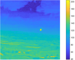
(a)

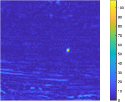
(b)

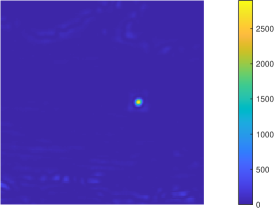
(c)

Figure 2: Variable dynamic range in saliency map. a) Original infrared image. b) filtering result using TopHat algorithm [14], c) filtering result using AAGD [37] algorithm. The dynamic range of the saliency map might be different than input infrared image depending on the applied IRSTD.

When the background noise is not strong, this automatic thresholding operation shows good performance for final target detection (3(d)). However, in strong noisy scenarios, the performance of this algorithm is degraded significantly (4(d)), which in turn, increases the false responses. Moreover, when infrared scenario does not contain any small target, these histogram-based automatic thresholding methods always return incorrect responses in non-target areas (Fig. 5).

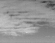
(a)

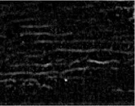
(b)

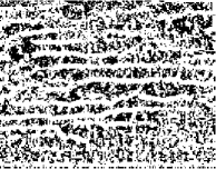
(c)

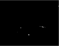
(d)

(e)

Figure 3: The automatic thresholding results. a) Original infrared image. b) Top-hat filtering result [14]. c) Otsu’s thresholding result $(T=0.48)$. d) automatic thresholding using average values of background and target classes $(T=19)$. e) Manual thresholding $(T=29)$.

Statistics-based image thresholding is the most effective thresholding strategy for small target detection which can be applied in both local and global manners. Statistics-based global and local thresholding are expressed in Eq. 4 and Eq. 5, respectively.

$$T=\mu_{G}+k_{G}\times\sigma_{G}$$ (4)

$$T(x,y)=\mu(x,y)+k_{L}\times\sigma(x,y)$$ (5)

where, $\mu_{G}$, $\sigma_{G}$, $\mu(x,y)$, $\sigma(x,y)$, $k_{G}$, and $k_{L}$ indicate global mean of the image, global standard deviation of the image, local mean around $(x,y)$ position, local standard deviation around $(x,y)$ position, control parameter of global thresholding and local thresholding, respectively.

Global thresholding is a simple operation with low computational complexity. However, in multi-target scenarios, some targets may be missed. Local thresholding can detect all targets. Since local mean and standard deviation should be calculated for each pixel in the gray image, the local statistics-based thresholding has higher computational complexity compared to the global one. Generally speaking, using statistics-based thresholding has the following advantages:

• It can work with any gray-level dynamic ranges.

• The control parameter $(k)$ can be determined by experiments to achieve reasonable false-alarm rate.

• The last but not the least, it is very effective for scenarios with no targets.

(a)

(b)

(c)

(d)

(e)

Figure 4: The automatic thresholding results. a) Original noisy infrared image. b) Top-hat filtering result. c) Otsu’s thresholding result $(T=0.5)$. d) automatic thresholding using average values of background and target classes $(T=7)$. e) Manual thresholding $(T=10)$.

(a)

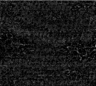
(b)

(c)

Figure 5: Drawback of automatic thresholding in scenarios with no targets. a) original infrared image which does not contain small target. b) the result of Top-Hat filtering. c) automatic thresholding results.

3 Pre-thresholding evaluation

A detection process is successful as long as a single pixel of target area is correctly recognized. In this case, the exact boundary extraction of the target area is not important at all. Therefore, a proper evaluation metric should support this argument.

Signal to clutter ratio (SCR) is one of pre-thresholding metrics which shows the target enhancement ability of an IRSTD, which is defined as:

$$SCR=\frac{\mu_{T}-\mu_{b}}{\sigma_{b}},$$ (6)

where, $\mu_{T}$, $\mu_{b}$, and $\sigma_{b}$ denote average intensity of the target area, average intensity and standard deviation of its local surrounding background, respectively. While this evaluation measure is generally accepted in the literature, it can not correctly reflect the target enhancement capability of an IRSTD. To better understanding, a simple scenario is provided here (Fig. 6).

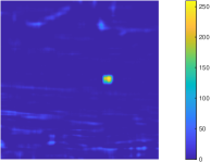
(a)

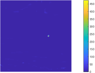
(b)

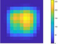
(c)

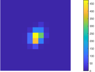
(d)

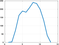
(e)

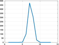
(f)

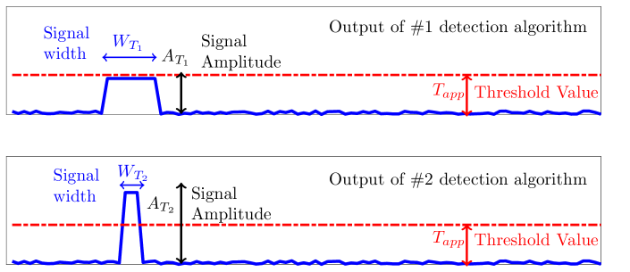
(g)

Figure 6: A simple scenario to demonstrate the drawback of common SCR metric. a, b) Saliency map of the IRSTD $\#1$ and $\#2$, c, d) target area in the saliency map of the IRSTD $\#1$ and $\#2$, e, f) $1$D plot of target cross-section in 6(c) and 6(d), g) simplified $1$D representation of target area in both IRSTD $\#1$ and $\#2$.

Two different saliency maps are demonstrated in 6(a) and 6(b). 6(a) shows the result of applying AAGD algorithm [37] with $9\times 9$ internal window. As depicted in the figure; the target area is relatively enhanced while there are some remaining background clutter. Compared to the 6(a), the second IRSTD which again is an AAGD 6(b) algorithm with $3\times 3$ internal window followed by a morphological erosion with a $3\times 3$ square-shape structural element, shows better target enhancement and background suppression. As shown in 6(c) and 6(d), the signal amplitude for the IRSTD $\#2$ is almost twice as the one in the IRSTD $\#1$, which means in higher threshold values the target will be detected corectly in the second one, while in the first one the target will be missed. One dimensional ($1$D) cross-section of target area in both saliency maps are shown in 6(e) and 6(f), respectively. To simplify the scenario, let’s approximate $1$D cross-section of the target area with closest square signal. The result is shown in 6(g). As shown in the figure:

$$A_{T_{1}}=\frac{A_{T_{2}}}{2}\quad,\quad W_{T_{1}}=3\times W_{T_{2}}$$ (7)

where, $A_{T_{1}}$, $A_{T_{2}}$ denote the target amplitude in the output of IRSTD $\#1$ and $\#2$. Also, $W_{T_{1}}$, $W_{T_{2}}$ show the target width (extension) in the output of IRSTD $\#1$ and $\#2$, respectively.

Based on SCR formulation (Eq. 6), and simply considering zero-mean background signal, the following relationship can be easily derived:

$$SCR_{1}=\frac{3}{2}\times SCR_{2}$$ (8)

which implies that the target detection ability of the IRSTD $\#1$ is $50\%$ more than that of IRSTD $\#1$. However, by applying a global threshold level at $T_{app}$, the $\#1$ algorithms does not detect the true target (Fig. 6). It can be clearly seen that the $\#2$ algorithm can detect the true target at the same threshold level. In order to address this issue when global thresholding is final choice in practical system, the SCR formulation should be modified as:

$$\boxed{SCR_{global}=\frac{\max_{T}-\mu_{G}}{\sigma_{G}}},$$ (9)

where, $\max_{T}$ denotes the maximum gray value of the target area. According to Eq. 4, the maximum acceptable control parameter is equal to newly defined SCR metric:

$$k_{G_{\max}}=SCR_{global}.$$ (10)

There are two important points regarding the Eq. 10:

1. Common SCR metric is not able to correctly reflect the target detection ability. The pre-thresholding evaluation should be performed in a global manner on the saliency maps.

2. The thresholding operation should be consistent with pre-thresholding evaluation metrics. For instance, in our case, the global statistics-based thresholding is the right choice.

So far, it is demonstrated that the global thresholding is the right one to be applied on the saliency map. In the next subsection, we demonstrate the drawback of the local statistics-based thresholding.

3.1 Drawback of common local thresholding

Now, let consider the case that local thresholding is supposed to be applied on the saliency map. According to Fig. 6, the local mean around target region can be calculated as follows:

$$\mu(x)=\frac{AW}{n}$$ (11)

where, $A$, $W$, $x$, and $n$ stand for the target amplitude, width (spatial extension), the current index and number of samples in local neighborhood ($n>W$).

The local standard deviation can be calculated as:

$$\sigma(x)=\sqrt{\frac{1}{n}\sum_{i=1}^{n}\left(y(i)-\mu(x)\right)^{2}}$$ (12)

Where $y(i)$ and $\mu(x)$ denote the saliency map samples and local mean, respectively. Since the detection algorithm is supposed to suppress background clutter, for the sake of simplicity, we can assume that the saliency map samples out of the target region are equal to zero. Then:

$$\sigma(x)=\frac{A}{n}\left(\sqrt{nW-W^{2}}\right)$$ (13)

The local thresholding (Eq. 5), can be rewritten as:

$$T(x)=\mu(x)+k_{L}\times\sigma(x)=\frac{AW}{n}+\frac{k_{L}A}{n}\left(\sqrt{nW-W^{2}}\right)$$ (14)

The detection process is established correctly for the threshold values lower than target amplitude ($T(x)<A$). Therefore, for a successful target detection the following condition should be met:

$$\begin{split}&\mu(x)+k_{L}\times\sigma(x)<A\\ &\Rightarrow\frac{AW}{n}+\frac{k_{L}A}{n}\left(\sqrt{nW-W^{2}}\right)<A\end{split}$$ (15)

The upper bound for control parameter ($k_{L_{\max}}$) to detect the target accurately can be find as follows:

$$\begin{split}&\frac{AW}{n}+\frac{k_{L_{\max}}A}{n}\left(\sqrt{nW-W^{2}}\right)=A\\ &\Rightarrow k_{L_{\max}}=\sqrt{\frac{n-W}{W}}\end{split}$$ (16)

Fig. 7 shows the upper bound of control parameter versus target width. As shown in the figure, the maximum control parameter to detect target correctly using local thresholding decreases as the target width increases. $k_{L_{\max}}$ takes its maximum value when the target width is equal to one pixel ($k_{L_{\max}}=\sqrt{n-1}$ for $W=1$). This result is quite consistent with the fact that the most effective target detection algorithm should suppress all background region and only returns a single pixel (Target centroid).

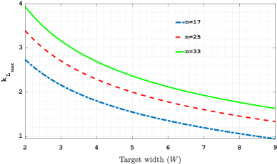
Figure 7: $k_{L_{\max}}$ versus target spatial extension $W$ (target width in $1$D case)

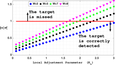
(a)

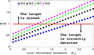
(b)

Figure 8: Local threshold value normalized to target amplitude ($\frac{T}{A}$) versus different control parameter. a) $n=33$, b) $n=17$.

Fig. 8 shows the local threshold value which is normalized to the target amplitude ($\frac{T}{A}$) versus different control parameter. It is clear that, only when the ($\frac{T}{A}$) fraction is less than one the target can be detected correctly. Another finding which can be derived from the figure is that the maximum control parameter decreases as the target width increases. Therefore, unlike the global case, the effective control parameter to extract real targets and eliminate background clutter depends on the target area in the saliency map. Also, the reasonable rang for control parameter is narrowed when the local neighborhood is decreased (8(b)). Moreover, using Eq. 5 to extract true target from saliency map leads to many false alarms. Fig. 9 shows the local thresholding on the saliency map of multi-scale Laplacian of Gaussian (LoG) method [18]. As shown in the 9(b), the target area is the most salient region in saliency map. However, after thresholding using local method (9(c)), there are too many false responses. The only way to limit false responses to an acceptable range is to increase the control parameter. However, the true target is not extracted when the local threshold is increased. Note that there are still too many false responses in 9(d).

(a)

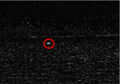
(b)

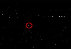
(c)

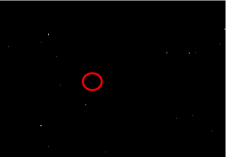
(d)

Figure 9: Shortcoming of local thresholding. a) Original input image, the target area is marked by red ellipse, b) the result of target enhancement using multi-scale Laplacian of Gaussian (LoG) method, c) the local thresholding applied on (b) with $k=4$, c) the local thresholding applied on (b) with $k=5$.

Based on the local thresholding results Fig. 9, this method (Eq. 5) is not a proper strategy to discriminate target area from background clutter.

4 Post-thresholding evaluation

After applying a predefined threshold to the saliency map, a binary image is obtained. In this case, the prevalent metrics to evaluate the performance of the detection algorithms are probability of false-alarm $P_{fa}$ and detection $P_{d}$. These two metrics are defined as [38]:

$$P_{fa}=\frac{N_{f}}{N_{tot}}\quad,\quad P_{d}=\frac{N_{d}}{N_{r}}$$ (17)

where $N_{f}$, $N_{tot}$, $N_{d}$, and $N_{r}$ denote the number of wrongly detected pixels, the total number of pixels, the number of pixels which are detected correctly, and the target pixels in the ground-truth, respectively. The receiver operational characteristics (ROC) curve is constructed by considering each $(P_{fa},P_{d})$ pair at different threshold level.

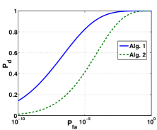
Figure 10: ROC curve for two typical detectors

Fig. 10 shows the ROC curve for two typical detectors. As shown in the figure, for a constant false-alarm rate, the detector $\#1$ has higher detection rate, and outperforms the algorithm $\#2$. The ROC curve is a satisfactory tool to evaluate the performance of different detectors. However, if the detection rate and false-alarm rate are not defined accurately, the final ROC curve is not a reliable measure anymore. In order to demonstrate the deficiency of the definitions of the $P_{d}$ and $P_{fa}$ (Eq. 17), let consider the target detection ability of two well-known small infrared target detection algorithms; Local contrast method (LCM) [23] and Top-hat algorithm [39]. Fig. 11 shows the detection results of these two algorithms. As shown in the figure, the Top-hat filtering method clearly outperforms the LCM algorithm. however, the ROC curve gives contradictory result against visual perception (12(a)). Also, by constructing the curve of the false-alarm rate versus different threshold levels (12(b)), the low performance of the LCM algorithm is clearly seen. Therefore, the former definition of the $P_{d}$ (Eq. 17) is not appropriate for this crucial metric.

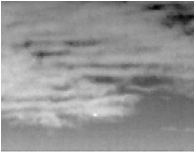
(a)

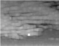
(b)

(c)

Figure 11: a) original image, b) the LCM filtering result, c) the Top-Hat filtering result.

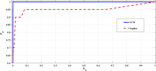
(a)

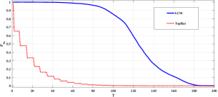
(b)

Figure 12: a) The ROC curve, b) false-alarm rate versus different threshold levels.

Another alternative definition for $P_{d}$ is suggested in the literature ([25]):

$$P_{d}=\frac{N_{D}}{N_{R}}$$ (18)

where $N_{D}$ and $N_{R}$ are number of detected true targets, and total number of true targets. While this new definition addresses the deficiency of the former one (Eq. 17), there are still some drawbacks regrading this formula; The real infrared scenarios usually contain limited number of targets. To overcome this drawback, synthetic targets are usually created using Gaussian spatial distribution. However, spatial distribution-based target detection algorithms directly benefit from synthetic data, so the final evaluation is not fair. An example is provided here to better demonstration of this situation. The character filter [40] utilizes Gaussian spatial distribution as a measure to distinguish between real target and background clutter. As shown in Fig. 13, when the small target has exactly Gaussian distribution, the character filter effectively can enhance the small targets and eliminate background clutter. However, in real infrared scenarios, which the spatial distribution of small targets does not follow the Gaussian distribution [38], the detection results of character filter is chaotic (Fig. 14).

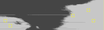
(a)

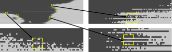
(b)

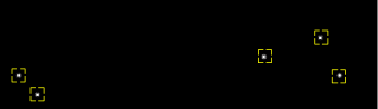
(c)

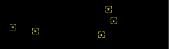
(d)

Figure 13: a) Synthetic targets in homogeneous local background, b) low contrast targets in background clutter edges, c) the character filter response to 13(a) and 13(b)).

(a)

(b)

(c)

(d)

Figure 14: a, c) real infrared scenario, b , d) the response of character filter [40] to 14(a) and 14(c), respectively.

According to aforementioned issues regarding the post-thresholding performance evaluation metrics, herein, awe present a new approach capable of addressing all the shortcomings. Since in a successful detection operation, at least one pixel is detected after thresholding operation, the following procedure is introduced to obtain new post-thresholding performance measure:

1. The upper bound for control parameter ($k_{\max}$) is calculated (Eq. 10).

2. The $[0-k_{max}]$ interval is chosen as valid interval for performance evaluation.

3. For each different control parameters, the false-alarm rate is calculated using Eq. 17.

4. The false-alarm rate versus control parameter ($P_{fa}$ – $k$) curve is constructed. In the next step, the $[0$ – $k]$ interval is linearly mapped to $[0$ – $1]$ range. This normalization allows us to fairly compare and evaluate different algorithms.

After constructing ($P_{fa}$ – $k$) curve, the following measures can be extracted:

• The maximum control parameter ($k_{\max}$) is the first inferred performance evaluation metric. The larger $k_{\max}$, the higher detection ability.

• The false-alarm rate at $k_{\max}$, which is called $P_{fa,\min}$ here, is the second evaluation metric. It is obvious that the false-alarm rate of the system can not be less than $P_{fa,\min}$ while the true target is detected.

After normalizing $[0$ – $k]$ interval to $[0$ – $1]$ range, the false alarm rate of the detection algorithms can be plotted in single figure. Then, the algorithm with satisfying detection performance can be chosen for the practical application.

5 Detection ability evaluation using new metrics

In order to evaluate the detection ability using the proposed metrics, four well-known small infrared target detection algorithms are chosen to conduct the experiments. Tab. 1 reports the baseline algorithms and their implementation details. The pre-thresholding enhancement results of each algorithm are depicted in Fig. 15. Visually speaking, the AAGD algorithm has better performance in background suppression (the background region is mapped to zero value). However, the most part of gray area in PCM output have zero values (Since there are also negative values in the saliency map, the zero values are depicted by gray color instead of black one). LoG and TopHat filters are sensitive to noise and sharp edges, therefore, there are too many false responses in their saliency maps.

The results of evaluation using new metrics are reported in Tab. 2 and Tab. 3. As reported in Tab. 2, AAGD and PCM algorithms have better enhancement for target area. However, by taking the false-alarms into account, the PCM algorithm shows better clutter rejection ability.

Table 1: The baseline algorithms

Detection Algorithm	Details
Top-Hat [39]	$7\times 7$ structural element
LoG [18]	With [0.50, 0.60, 0.72, 0.86, 1.03, 1.24, 1.49, 1.79, 2.14, 2.57, 3.09, 3.71] scale parameters
PCM [41]	With [$3\times 3$, $5\times 5$, $7\times 7$, and $9\times 9$] cell-sizes
AAGD [42]	With [$3\times 3$, $5\times 5$, $7\times 7$, and $9\times 9$] cell-sizes

(a)

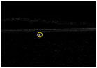
(b)

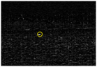
(c)

(d)

(e)

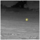
(f)

(g)

(h)

(i)

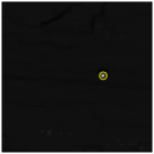
(j)

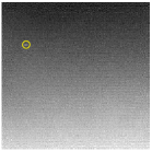
(k)

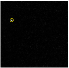
(l)

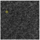
(m)

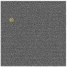
(n)

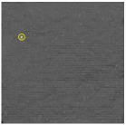
(o)

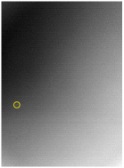
(p)

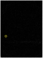
(q)

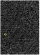
(r)

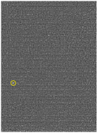
(s)

(t)

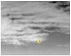
(u)

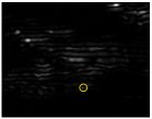
(v)

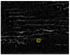
(w)

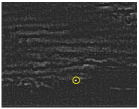
(x)

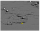
(y)

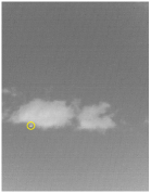
(z)

(aa)

(ab)

(ac)

(ad)

Figure 15: Pre-thresholding results of the algorithms under the test on real infrared images (Target region is marked by yellow circle). From the left: the first column: original images, the second column: filtering results of AAGD algorithm, the third column: filtering results of Tophat transform, the fourth column: filtering results of LoG algorithm, the fifth column: filtering results of PCM algorithm.

Table 2: The value of maximum control parameter $k_{max}$ for different algorithms

	the $1^{st}$ test image	the $2^{nd}$ test image	the $3^{rd}$ test image	the $4^{th}$ test image	the $5^{th}$ test image	the $6^{th}$ test image
AAGD	39.8553	61.9809	45.8804	57.9033	8.0117	166.4851
LoG	16.5312	28.8976	5.4743	7.2515	13.4517	37.4031
TopHat	15.8858	22.8994	2.5513	3.8742	14.4408	26.9160
PCM	13.7368	67.1190	25.5538	14.4819	12.4008	87.0127

Table 3: The value of minimum probability of false alarm $P_{fa,\min}$ for different algorithms

	$1^{st}$ test image	$2^{nd}$ test image	$3^{rd}$ test image	$4^{th}$ test image	$5^{th}$ test image	$6^{th}$ test image
AAGD	0	0	7.4627e-5	1.3412e-5	0.0019	0
LoG	0	0	7.4627e-5	5.3648e-5	0	0
TopHat	0	0	0.0044	1.7436e-4	0	0
PCM	0	0	0	1.3412e-5	0	0

Finally, Fig. 16 shows the normalized ($P_{fa}$ – $k$) curve to investigate the detection performance characteristics of different baseline algorithms, and fairly compare them. As shown in the figure, the PCM and AAGD algorithm has overall superiority compared to LoG and TopHat algorithms. The AAGD algorithm shows poor detection performance in the $5^{th}$ test image (Fig. 15). As shown in 16(e), the new metrics is completely consistent with the visual and qualitative results (Fig. 15).

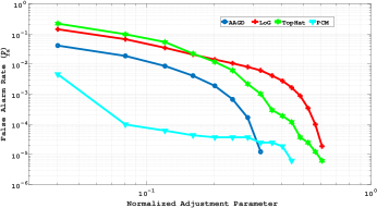
(a)

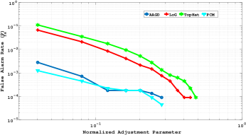
(b)

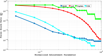
(c)

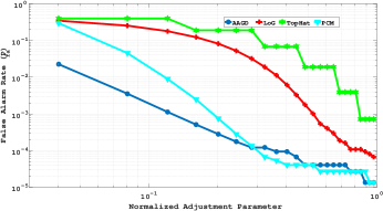
(d)

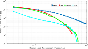
(e)

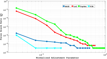
(f)

Figure 16: The normalized ($P_{fa}$ – $k$) curve in logarithmic scale. The detection performance characteristics curve for: a) the $1^{st}$ test image, b) the $2^{nd}$ test image, c) the $3^{rd}$ test image, d) the $4^{th}$ test image, e) the $5^{th}$ test image, f) the $6^{th}$ test image.

6 Conclusion

The development of new algorithms for infrared small target detection is attracted more attention during the last decade. However, many of these recently developed algorithms do not meet the requirements of the practical applications. Also, there are some disadvantage regarding the common evaluation metrics. In order to completely understand the requirements of the effective evaluation metrics, the practical procedure of small target detection should be revealed. The thresholding operation has a great role in this procedure. Without a proper thresholding strategy, the previous efforts in target enhancement algorithm development would become obsolete. It has been demonstrated that the local statistics-based thresholding is not an appropriate option for the segmentation of saliency map, and the the global statistics-based threshold operation is better choice.

By considering the global thresholding as final step for the detection algorithm, the signal to clutter ratio (SCR) metric is modified for better detection ability reflection. Also, three post-thresholding metrics are proposed to complete performance evaluation of different algorithms.

References

- [1] M. Chudecka, A. Dmytrzak, K. Leźnicka, and A. Lubkowska, “The use of thermography as an auxiliary method for monitoring convalescence after facelift surgery: A case study,” International Journal of Environmental Research and Public Health, vol. 19, no. 6, p. 3687, 2022.
- [2] S. Moradi, J. Moradi, S. Aghaziyarati, and H. Shahraki, “Infrared image enhancement based on optimally weighted multi-scale laplacian of gaussian and local statistics using particle swarm optimization,” International Journal of Image and Graphics, p. 2450014, 2022.
- [3] A. Choudhary, T. Mian, and S. Fatima, “Convolutional neural network based bearing fault diagnosis of rotating machine using thermal images,” Measurement, vol. 176, p. 109196, 2021.
- [4] H. Shahraki, S. Aalaei, and S. Moradi, “Infrared small target detection based on the dynamic particle swarm optimization,” Infrared Physics & Technology, vol. 117, p. 103837, 2021.
- [5] A. Raza, J. Liu, Y. Liu, J. Liu, Z. Li, X. Chen, H. Huo, and T. Fang, “Ir-msdnet: Infrared and visible image fusion based on infrared features and multiscale dense network,” IEEE Journal of Selected Topics in Applied Earth Observations and Remote Sensing, vol. 14, pp. 3426–3437, 2021.
- [6] M. Zhang, R. Zhang, Y. Yang, H. Bai, J. Zhang, and J. Guo, “Isnet: Shape matters for infrared small target detection,” in Proceedings of the IEEE/CVF Conference on Computer Vision and Pattern Recognition, 2022, pp. 877–886.
- [7] H. Shahraki, S. Moradi, and S. Aalaei, “Infrared target detection based on the single-window average absolute gray difference algorithm,” Signal, Image and Video Processing, vol. 16, no. 3, pp. 857–863, 2022.
- [8] S. Moradi, P. Moallem, and M. F. Sabahi, “Fast and robust small infrared target detection using absolute directional mean difference algorithm,” Signal Processing, vol. 177, p. 107727, 2020.
- [9] P. Khaledian, S. Moradi, and E. Khaledian, “A new method for detecting variable-size infrared targets,” in Sixth International Conference on Digital Image Processing (ICDIP 2014), vol. 9159. International Society for Optics and Photonics, 2014, p. 91591J.
- [10] X.-h. Bai, S.-w. Xu, Z.-x. Guo, and P.-l. Shui, “Floating small target detection based on the dual-polarization cross-time-frequency distribution in sea clutter,” Digital Signal Processing, vol. 129, p. 103625, 2022.
- [11] M. Zhao, W. Li, L. Li, J. Hu, P. Ma, and R. Tao, “Single-frame infrared small-target detection: A survey,” IEEE Geoscience and Remote Sensing Magazine, 2022.
- [12] S. D. Deshpande, M. H. Er, R. Venkateswarlu, and P. Chan, “Max-mean and max-median filters for detection of small targets,” in Signal and Data Processing of Small Targets 1999, vol. 3809. SPIE, 1999, pp. 74–83.
- [13] T.-W. Bae, “Spatial and temporal bilateral filter for infrared small target enhancement,” Infrared Physics & Technology, vol. 63, pp. 42–53, 2014.
- [14] H. Zhu, J. Zhang, G. Xu, and L. Deng, “Balanced ring top-hat transformation for infrared small-target detection with guided filter kernel,” IEEE Transactions on Aerospace and Electronic Systems, vol. 56, no. 5, pp. 3892–3903, 2020.
- [15] J. Han, S. Liu, G. Qin, Q. Zhao, H. Zhang, and N. Li, “A local contrast method combined with adaptive background estimation for infrared small target detection,” IEEE Geoscience and Remote Sensing Letters, vol. 16, no. 9, pp. 1442–1446, 2019.
- [16] X. Wang, Z. Peng, P. Zhang, and Y. He, “Infrared small target detection via nonnegativity-constrained variational mode decomposition,” IEEE Geoscience and Remote Sensing Letters, vol. 14, no. 10, pp. 1700–1704, 2017.
- [17] Q. Wang, G. Liu, and Y. Shi, “Detecting of multi-dim-small-target in sea or sky background based on higher-order cumulants and wavelet,” in Recent Advances in Computer Science and Information Engineering. Springer, 2012, pp. 497–504.
- [18] S. Kim and J. Lee, “Scale invariant small target detection by optimizing signal-to-clutter ratio in heterogeneous background for infrared search and track,” Pattern Recognition, vol. 45, no. 1, pp. 393–406, 2012.
- [19] X. Wang, G. Lv, and L. Xu, “Infrared dim target detection based on visual attention,” Infrared Physics & Technology, vol. 55, no. 6, pp. 513–521, 2012.
- [20] J. Han, Y. Ma, J. Huang, X. Mei, and J. Ma, “An infrared small target detecting algorithm based on human visual system,” IEEE Geoscience and Remote Sensing Letters, vol. 13, no. 3, pp. 452–456, 2016.
- [21] K. Xie, K. Fu, T. Zhou, J. Zhang, J. Yang, and Q. Wu, “Small target detection based on accumulated center-surround difference measure,” Infrared physics & technology, vol. 67, pp. 229–236, 2014.
- [22] L. Li, Z. Li, Y. Li, C. Chen, J. Yu, and C. Zhang, “Small infrared target detection based on local difference adaptive measure,” IEEE Geoscience and Remote Sensing Letters, vol. 17, no. 7, pp. 1258–1262, 2019.
- [23] C. P. Chen, H. Li, Y. Wei, T. Xia, and Y. Y. Tang, “A local contrast method for small infrared target detection,” IEEE Transactions on Geoscience and Remote Sensing, vol. 52, no. 1, pp. 574–581, 2013.
- [24] J. Han, Y. Ma, B. Zhou, F. Fan, K. Liang, and Y. Fang, “A robust infrared small target detection algorithm based on human visual system,” IEEE Geoscience and Remote Sensing Letters, vol. 11, no. 12, pp. 2168–2172, 2014.
- [25] J. Han, K. Liang, B. Zhou, X. Zhu, J. Zhao, and L. Zhao, “Infrared small target detection utilizing the multiscale relative local contrast measure,” IEEE Geoscience and Remote Sensing Letters, vol. 15, no. 4, pp. 612–616, 2018.
- [26] J. Han, S. Moradi, I. Faramarzi, C. Liu, H. Zhang, and Q. Zhao, “A local contrast method for infrared small-target detection utilizing a tri-layer window,” IEEE Geoscience and Remote Sensing Letters, vol. 17, no. 10, pp. 1822–1826, 2019.
- [27] Y. Qin, L. Bruzzone, C. Gao, and B. Li, “Infrared small target detection based on facet kernel and random walker,” IEEE Transactions on Geoscience and Remote Sensing, vol. 57, no. 9, pp. 7104–7118, 2019.
- [28] J. Han, S. Moradi, I. Faramarzi, H. Zhang, Q. Zhao, X. Zhang, and N. Li, “Infrared small target detection based on the weighted strengthened local contrast measure,” IEEE Geoscience and Remote Sensing Letters, vol. 18, no. 9, pp. 1670–1674, 2020.
- [29] J. Han, Q. Xu, S. Moradi, H. Fang, X. Yuan, Z. Qi, and J. Wan, “A ratio-difference local feature contrast method for infrared small target detection,” IEEE Geoscience and Remote Sensing Letters, vol. 19, pp. 1–5, 2022.
- [30] C. Gao, D. Meng, Y. Yang, Y. Wang, X. Zhou, and A. G. Hauptmann, “Infrared patch-image model for small target detection in a single image,” IEEE transactions on image processing, vol. 22, no. 12, pp. 4996–5009, 2013.
- [31] Y. Dai, Y. Wu, and Y. Song, “Infrared small target and background separation via column-wise weighted robust principal component analysis,” Infrared Physics & Technology, vol. 77, pp. 421–430, 2016.
- [32] Y. Dai, Y. Wu, Y. Song, and J. Guo, “Non-negative infrared patch-image model: Robust target-background separation via partial sum minimization of singular values,” Infrared Physics & Technology, vol. 81, pp. 182–194, 2017.
- [33] L. Zhang, L. Peng, T. Zhang, S. Cao, and Z. Peng, “Infrared small target detection via non-convex rank approximation minimization joint l 2, 1 norm,” Remote Sensing, vol. 10, no. 11, p. 1821, 2018.
- [34] T. Zhang, H. Wu, Y. Liu, L. Peng, C. Yang, and Z. Peng, “Infrared small target detection based on non-convex optimization with lp-norm constraint,” Remote Sensing, vol. 11, no. 5, p. 559, 2019.
- [35] N. Otsu, “A threshold selection method from gray-level histograms,” IEEE transactions on systems, man, and cybernetics, vol. 9, no. 1, pp. 62–66, 1979.
- [36] R. Gonzalez and R. Woods, Digital Image Processing. Pearson Education, 2011.
- [37] S. Moradi, P. Moallem, and M. F. Sabahi, “A false-alarm aware methodology to develop robust and efficient multi-scale infrared small target detection algorithm,” Infrared Physics & Technology, vol. 89, pp. 387–397, 2018.
- [38] ——, “Scale-space point spread function based framework to boost infrared target detection algorithms,” Infrared Physics & Technology, vol. 77, pp. 27–34, 2016.
- [39] V. T. Tom, T. Peli, M. Leung, and J. E. Bondaryk, “Morphology-based algorithm for point target detection in infrared backgrounds,” in Signal and Data Processing of Small Targets 1993, vol. 1954. International Society for Optics and Photonics, 1993, pp. 2–11.
- [40] R. Hu, X. Zhou, G. Zhang, and G. Zhang, “Infrared dim target detection based on character filter,” in MIPPR 2011: Automatic Target Recognition and Image Analysis, T. Zhang and N. Sang, Eds., vol. 8003, International Society for Optics and Photonics. SPIE, 2011, pp. 319 – 325.
- [41] Y. Wei, X. You, and H. Li, “Multiscale patch-based contrast measure for small infrared target detection,” Pattern Recognition, vol. 58, pp. 216–226, 2016.
- [42] H. Deng, X. Sun, M. Liu, C. Ye, and X. Zhou, “Infrared small-target detection using multiscale gray difference weighted image entropy,” IEEE Transactions on Aerospace and Electronic Systems, vol. 52, no. 1, pp. 60–72, 2016.