Quantifying Rare Events in Stochastic Reaction-Diffusion Dynamics Using Tensor Networks
Abstract
The interplay between stochastic chemical reactions and diffusion can generate rich spatio-temporal patterns. While the timescale for individual reaction or diffusion events may be very fast, the timescales for organization can be much longer. That separation of timescales makes it particularly challenging to anticipate how the rapid microscopic dynamics gives rise to macroscopic rates in the non-equilibrium dynamics of many reacting and diffusing chemical species. Within the regime of stochastic fluctuations, the standard approach is to employ Monte Carlo sampling to simulate realizations of random trajectories. Here, we present an alternative numerically tractable approach to extract macroscopic rates from the full ensemble evolution of many-body reaction diffusion problems. The approach leverages the Doi-Peliti second-quantized representation of reaction-diffusion master equations along with compression and evolution algorithms from tensor networks. By focusing on a Schlögl model with one-dimensional diffusion between otherwise well-mixed sites, we illustrate the potential of the tensor network approach to compute rates from many-body systems, here with approximately microstates. Specifically, we compute the rate for switching between metastable macrostates, with the expense for computing those rates growing subexponentially in . Because we directly work with ensemble evolutions, we crucially bypass many of the difficulties encountered by rare event sampling techniques—detailed balance and reaction coordinates are not needed.
I Introduction
Connecting microscopic kinetics to emergent rates has a long history for equilibrium and nonequilibrium processes. Complex systems often settle into metastable basins with rare transitions regulating the rates of switching between the emergent states. In equilibrium, transition state theory [1, 2], variational transition state theory [3], Grote-Hynes theory [4, 5], and transition path sampling (TPS) [6, 7] have given strategies to estimate the transition rate. Away from equilibrium, theories built upon a free energy landscape lose their applicability, yet trajectory sampling approaches can extract rates from microscopic dynamics, through noise-guided TPS approach [8, 9] or forward flux sampling (FFS) [10, 11, 12]. For all their merits, sampling approaches bring intrinsic challenges. How many samples are required to estimate the rate? Is a good approximate reaction coordinate needed, and if so, how is it found [13]? How does the expense grow with larger or more complicated microscopic systems? Motivated by those ubiquitous concerns, we set out to consider a different approach—one that effectively samples all possible trajectories as an ensemble evolution instead of propagating individual realizations. Such a proposition may appear absurd given the exploding state space presented by the many-body problem, but we show that for the class of discrete state, continuous-time, reaction-diffusion master equations (RDME), we can evolve the full distribution of a classical many-body systems in a numerically controllable manner by combining two well-developed methods, the Doi-Peliti (DP) formalism with tensor network (TN) algorithms.
While TPS and FFS have been developed for a variety of dynamical equations of motion (Hamiltonian, Langevin, Markov jump, etc.), we focus our attention solely on the chemical master equation (CME) dynamics, the setting where FFS was first developed [10]. More specifically, we study discrete reaction-diffusion dynamics of sites or voxels as they are often called in the RDME literature [14, 15]. The rationale for this focus is twofold. From a practical perspective, the RDME is important as a popular method to model chemical and biological processes [16, 17, 18]. From a theoretical perspective, the RDME is interesting because it provides a setting where one can analyze the influence of stochasticity on the emergence of patterns [19, 20, 21]. In many pattern-formation problems, it is possible to understand the underlying physics in terms of a mean-field partial differential equation that tracks spatiotemporal evolution of deterministically evolving fields [22, 23]. It is, however, well-appreciated that stochastic effects can quantitatively and even qualitatively impact kinetics [24, 25, 26, 27, 28, 29, 25]. It is therefore important that the methodology we discuss captures more than just the typical dynamics. Accurately computing transition rates between metastable states requires quantitatively resolving even rare tails of the state space distribution since these rare fluctuations can be instrumental in triggering transitions [30, 11].
Historically, similar schemes for the CME ensemble evolution have been hampered by the curse of dimensionality. As a result, exact solutions are rare [31] and numerical solutions often resort to sampling methods built upon the kinetic Monte-Carlo stochastic simulation algorithm (SSA) [32, 33], also known as the Gillespie algorithm. Another approach is to evolve a subset of the state space through the finite state projection (FSP) method [34]. FSP has previously been combined with TNs to approximately describe the CME [35, 36], resembling our use of TNs to tame the many-body problem. Unlike those projective methods, however, the approach we describe uses the time-dependent variational principle (TDVP) to evolve the dynamics with probability conservation at all times, akin to prior work with diffusion and no reactions [37, 38, 39]. Since we estimate rare events by measuring the distribution’s small probability fluxes, conservation of probability and high-fidelity dynamical evolution are materially important.
While the formalism we describe applies quite generally to different well-mixed and reaction-diffusion models, we center our paper around a single model problem: rate calculations for transitions between basins of the Schlögl model [40] in the bistable regime, both with and without diffusion [41]. In Sec. II, we first illustrate the rare event problem and extract rate constants from a propagator in the well-mixed regime. For more complicated systems (either systems with more chemical species or more voxels), the curse of dimensionality precludes the exact calculation of the propagator, but the remainder of the paper shows how to employ TNs to follow the same conceptual path. In Sec. III, we review the Doi-Peliti framework for writing reaction-diffusion dynamics in a second-quantized field theoretic form. Sec. IV then reviews the TN matrix product state (MPS) ansatz, a controllable approximation to the ensemble that can be evolved via TDVP. Those methods are applied to the many-body rate calculation in Sec. V. In Sec. VI, we show results for the RDME with diffusion between well-mixed Schlögl voxels, demonstrating that the methodology can extend numerical transition rate calculations to regimes where the SSA becomes impractical. The approach effectively evolves the probability of occupying each microstate in an unfathomably large many-body state space, yet the calculations scale sub-exponentially with system size and do not assume detail-balanced equilibrium. Sec. VII discusses how the TDVP calculations yield not only a rate, but also a mechanism. Finally, in Sec. VIII, we discuss potential applications and challenges that should motivate future work.
II Ensemble rate calculations
Consider an archetypal two-state rate process between reactants and products , initiated entirely in the reactant state. After some reaction timescale, the concentration of products grows before eventually leveling off at its steady-state value. The reaction rate can simply be defined and measured in terms of how quickly the product concentration rises. An alternative formulation is to study the fate of an individual reactant on its path to transitioning into a product. The TPS and FFS path sampling approaches extract the reaction rate by focusing on the statistical properties of these individual trajectories. Algorithms exist to propagate those single trajectories, algorithms that can be practically implemented even when the system grows large and complex. By contrast, propagating the entire ensemble of trajectories has typically been limited to simple low-dimensional problems. In this section, we illustrate an ensemble-evolution rate calculation for a simple case in order to develop notation and lay the groundwork for the many-body problem. The remainder of the paper will show that the methodology can be extended beyond such simple problems by employing TNs.
II.1 Well-mixed Schlögl Model
Consider the well-mixed Schlögl model, a quintessential example of bistability in chemical reaction networks (CRNs) [42, 43]. The model tends to be studied under chemostatted conditions that fix two species’ concentrations and , while allowing species X’s concentration to evolve according to the four reactions:
where and are the stochastic rate coefficients. Our starting point is microscopic such that the rate should be interpreted as the reciprocal of the waiting time for a particular set of X molecules to react and form 3 X molecules when mediated by a fixed concentration of A molecules. In the large-system, well-mixed limit of chemical kinetics, it is common to also define macroscopic, or kinetic rate constants for each reaction with reactants. Here, Avogadro’s number serves to convert between microscopic measures (counting molecules) and macroscopic kinetic measures (concentrations in molarity) for a volume . In this paper, we focus on the microscopic kinetic picture, viewing the as the fundamental parameters, but these parameters can be converted into for linear reactions or in the thermodynamic limit [44]. In that thermodynamic limit, the stochastic kinetics often tends to the solutions of the deterministic reaction rate equations. For the Schlögl model, analysis of that deterministic limit reveals that the sign of the discriminant
| (1) |
determines the number of stable steady-state solutions [42]. While holding the rate coefficients fixed, the sign of changes as a function of the concentrations of A and B, allowing one to pass from with one steady-state solution, through with a diverging variance of the number of X molecules [45], and on to with one unstable and two stable solutions. In the regime, a finite (stochastic) system sees the regions around the two stable fixed points become metastable states. The number of X molecules stochastically switches between the two metastable values. A representative trajectory, shown in Fig. 1, oscillates between a state with X molecules and another with . We first set out to compute the rate of bistable switching between those two metastable states in the well-mixed regime, making use of the fact that the dynamics is one-dimensional (1D)— executes a random walk between 0 and some large maximum number , which we impose for the sake of calculation.
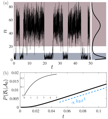
Rather than track for a single trajectory as in Fig. 1, the ensemble approach tracks evolution of the distribution , measuring the probability that an individual trajectory would have molecules at time . Foreshadowing the analogies with quantum-mechanical methodologies, we choose to write that distribution as a ket: , where indicates the transpose to give a column vector. The distribution evolves according to the master equation
| (2) |
Here, is a rate matrix whose off-diagonal elements are the rates of transitioning from X molecules to and whose diagonal elements are minus the rate of escaping from the state with X molecules. The rate matrix conserves probability, a fact compactly expressed as , with denoting a vector of ones. The distribution can always be formally evolved in terms of a propagator as
| (3) |
Due to the analogy with quantum-mechanical time evolution, we equivalently call an effective Hamiltonian. Assuming is irreducible, the long-time limit for this distribution tends to the unique steady-state .
can be decomposed into contributions from the two different reversible mechanisms of Eqs. (II.1) and (II.1), labeled and , respectively, based on whether the transitions are mediated by the chemostatted species A or B. Then, the Schlögl model at the level of the master equations corresponds to tridiagonal rate matrices with elements
| (4) |
and
| (5) |
where and is the Kronecker delta. Given the specific tridiagonal and the restriction , both and the propagator are matrices, amenable to evolving the entire distribution, effectively averaging over all the realizations.
To extract a rate from the evolution of distribution, we must initialize the distribution in one of the two metastable states and measure the rate of relaxation. In analogy with free energy basins, we will call the two metastable regions basins and (red and blue regions of Fig. 1 respectively) with . We write for the non-negative idempotent () operator that projects onto the density lying in a region , where . If has support over a state space , then the projection is an unnormalized distribution with support restricted to . The total probability in at time can then be expressed as .
II.2 Rate Constants
In general, one can compute the probability to pass from any subset into an arbitrary non-overlapping subset . For the current example, and are basins of attraction for the Schlögl model (see Fig. 1a), and we would like to measure the rate of going from . Rate constants can be defined either for the unidirectional flux from , the quantity we focus on in this work, or for the timescale of the relaxation to the steady-state, which also involves the transitions [46]. Additionally, the precise definition of the rate depends on whether one seeks trajectories that move from the boundary of one basin to another or from the interior of one basin to another. For instance, studying the time to transition from the boundary of to the boundary of yields the Transition Path Theory (TPT) rate associated with the committor function [47]. This unidirectional rate is related to the probability of having reached from in time without returning to . If we focus on trajectories short enough that those reaching will stay (no recrossings) then can be expressed in terms of the probability to start in at time zero and the conditional probability to subsequently be found in at time :
| (6) |
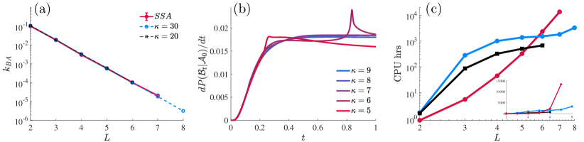
The derivative is evaluated at some timescale exceeding , a molecular time scale of the system that is long enough for the first trajectories to reach from but much shorter than the typical transit time (see Fig. 1b).
We compute the rate of Eq. (6) by initializing in a distribution confined to then propagating for time and measuring the probability in . A suitable initial distribution is , a normalized distribution constructed by projecting the steady-state distribution onto . With this contribution, , and Eq. (6) becomes
| (7) |
To the extent that there is a separation of timescales between exploring a basin and transiting between basins, the transition event is rare and no transitions can occur faster than the molecular time scale . Beyond that time, the number of transitions accumulates over time as . At times long compared to , must eventually stop growing linearly to level off at the stationary value , but our interest is in extracting from the growth at much shorter times. A typical realization of the process will not require observation much beyond units of time, to ascertain the rate, meaning our ensemble evolutions must be propagated for roughly . Notice from the inset of Fig. 1(b) that at long times the recrossing events obscure the rate of growth, ultimately yielding the plateau. As discussed in Sec. V and App. D, for rare rates and long times, the rate calculations can be improved by removing these recrossing events via a modified dynamics in which region is an absorbing state, forbidding dynamics out of that region.
Our ability to compute from the ensemble evolution traces back to the fact that it is practical to numerically calculate for the well-mixed model with a single species and a modest . While Eq. 7 generalizes naturally for harder problems (those with more than one species or with diffusion between multiple well-mixed voxels), the state space for grows exponentially with additional stochastic degrees of freedom. We next show that the Doi-Peliti framework re-expresses the rate matrix in a second-quantized form that allows us to generalize beyond the case of a single well-mixed species.
III Doi-Peliti
The Doi-Peliti (DP) formalism is a classical version of the second quantization methods from quantum field theory [48, 49]. Originally introduced by Doi [50] as a critique to the assumptions of the Smoluchowski equation, it was later developed by Peliti [51] and others [52] as a path integral formalism for solving chemical reaction networks [53, 54, 55, 56]. The DP framework has also found success in other areas such as studying kinetically constrained lattice models in the context of glassy dynamics [57, 58], cellular signaling [59], predator prey models [60] and active matter [61]. The DP representation builds operators which encode the dynamics onto the high-dimensional space that accompanies many-body problems. Crucially, writing the chemical reactions in an operator form guarantees it can be easily converted into a matrix product operator (MPO) [62, 63], as we will do in Sec. IV.
To start, we go beyond Sec. II by considering well-mixed reactions with multiple dynamic species as well as heterogeneous systems where molecules can diffuse between neighboring voxels. Let represent each chemical species in each site. We could be talking about a single species with different values in different voxels, a single well-mixed voxel with distinct dynamic species, or a mixture with multiple species and multiple voxels. The number of molecules in a given voxel can change due to a chemical reaction or a diffusion event, with both events being cast as,
| (8) |
where are again the rate coefficients for reaction . and reflect the stochiometry of the reactions and give the stochiometric vector which evolves the system from state to . In the previous section, these reactions induced changes between the different microstates, specified by the scalar . Now, the microstates are specified by , counting the occupation of each species within each voxel.
For a dilute well-mixed solution, where well-mixed means molecules locations within a voxel are unresolved, the change in probability of microstate follows the gain-loss equation [14],
| (9) |
where the sum is taken over different reactions of the form Eq. (8), each with their own stochiometric vector . The transition rate between any two states is the sum of contributions from each reaction . Each propensity is a product of a stochastic rate coefficient and the combinatorial number of ways to select either or molecules from reaction , depending on the direction of the reaction. For a “forward” reaction the propensity is, .
Encoding the reactions into a matrix form allows us to evolve the elements of the joint distribution analogously to the previous section. While it is appealing to try and directly solve these more complicated dynamics as we did before, it is impractical. The curse of dimensionality demands a less onerous way to work with both and . Since particles of the same species in the same voxel are indistinguishable, it is beneficial to work in an occupation number representation with
| (10) |
The basis vectors
| (11) |
corresponds to a possible microstate, and the set of basis vectors forms a tensor product space called a Fock space with and [64]. Without loss of generality, we will discuss the case of a single chemical species and physical voxels, in which case has the interpretation of the number of molecules in voxel . The second-quantization procedure rewrites the rate matrix as an operator in terms of creation and annihilation operators, and , that respectively raise and lower the number of X molecules in voxel . That is to say,
| (12) |
where is the vacuum state, i.e., no molecules. By or we are implying that the operator only acts on the voxel:
| (13) |
Because they act on the single-site space, the general one-site operators and can be written in a matrix form as
| (14) |
That these matrices yield Eq. (12) can be readily confirmed. More abstractly, the existence of such creation and annihilation operators in this classical setting originates from the classical commutation relation and the existence of a positive semi-definite number operator , so named because . Together, the set are also sometimes called an interacting Fock space [48]. As in the construction of the number operator, we will be able to decompose contributions to in terms of the and ’s.
In practice, the matrices of Eq. (14) will not be infinite in size but will rather be matrices due to our enforcement of a maximum voxel occupancy of . At the operator level, this maximum voxel occupancy supplements Eqs. (12) with an additional requirement that
| (15) |
a requirement that is met by the finite truncation of Eqs. (14). Those truncated operators obey a commutation relation which is similar to that of their infinite counterpart, but the usual commutation relation is broken at the maximal occupancy state. That is to say
| (16) |
The commutation relation for the truncated operators is therefore
| (17) |
an expression involving the projector operator onto site ’s maximal occupancy state, . As discussed in depth in App. A, this violation of the usual commutator relation must be accounted for when constructing an effective Hamiltonian that conserves probability.
One benefit of defining operators in terms of creation and annihilation operators is that expectation values for observables can be expressed easily in terms of inner products with operators. Consider, for example, the observable that counts all particles in all voxels, . The operator acts on a many-body state , yet each is a single-body operator acting on voxel and leaving all other voxels unchanged. It is therefore understood that when local operators such as act on , it is written as a shorthand for
| (18) |
In terms of that shorthand, counts the number of particles in voxel for the many-body state . The time-dependent expected number of particles in the whole system is thus , where the vector of ones serves to sum over all microstates. The time-dependence of a distribution can also be extracted from the action of a second-quantized on , and this operation can be practically computed when is expressed in terms of the single-site operators.
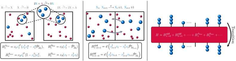
Mirroring the discussion in Sec. II, the generator for the Schlögl model reactions within the voxel is a sum of contributions from the elementary reactions . Fig. 2a shows each reaction, expressed as a second-quantized contribution to the effective Hamiltonian, as derived in App. A. Probability conservation requires that this effective Hamiltonian include a term with a projector that prevents flows of probability into forbidden microstates with occupancy greater than . This projector is complementary to the one appearing in Eq. (17) in that it projects onto states which are not maximally occupied. Combining together the forward and reverse reactions mediated by species A, we show in App. A that the reversible reaction Eq. (II.1) contributes
| (19) |
to the effective Hamiltonian. For convenience we have absorbed the combinatorial terms into that rate coefficient, defining , where is either or for forward and reversed reactions, respectively. Likewise, the contribution
| (20) |
comes from Eq. (II.1). In the limit, to give the more familiar expressions written in Fig. 2a.
The Hamiltonian operator for independent, well-mixed Schlögl voxels is thus . To add diffusion, consider the well-mixed voxels arranged in a 1D lattice as in Fig. 2b. Each chemical species is able to move between neighboring voxels as regulated by a diffusion operator
| (21) |
with hopping rate , consistent with macroscopic diffusion constant for voxel width [18]. Combining reaction with diffusion gives
| (22) |
a straightforward linear superposition at the level of the effective Hamiltonian. We emphasize that the linear superposition of diffusion with reactions and does not imply a restriction to linear kinetics. The Schlögl model kinetics is nonlinear in that it involves elementary reactions which are not first order, and the diffusive coupling between neighbors can induce nontrivial interactions between voxels.
IV Tensor Networks
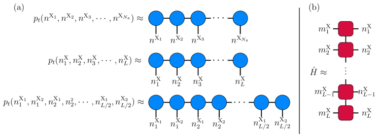
We have now seen how to transform the matrix-form rate operator of Sec. II into a Doi-Peliti form , expressed in terms of local creation and annihilation operators. That change of representation is not merely cosmetic. As the number of chemical species or number of lattice sites grows, the size of grows exponentially. For dynamical (unchemostatted) species and lattice sites, the state space has states. To put this scaling in perspective, the largest numerical result that follows uses , and , meaning the system contains microstates. Calculations on a matrix , even a very sparse matrix , are untenable. By contrast, it is practical to construct a TN decomposition of the second quantized form of in terms of an MPO, as shown in Fig. 3b, and demonstrated explicitly for the Schlögl model in App. B. Given the second quantized form, the MPO can be readily constructed in a practical form through SVD decomposition using automated packages such as AutoMPO in ITensor [65].
Much like the operator can be compressed as an MPO, the states that operators act upon can also be expressed more compactly in terms of TNs. Consider , the probability of microstate at time . This can be thought of as a rank tensor. By specifying the occupancy of each of the sites, outputs a number—a probability—associated to that microstate. By leveraging a matrix product ansatz, can be approximated as a partial contraction over different low-rank tensors (see Fig. 3a). The low rank tensors of an MPS [66] are organized in a 1D chain of site dependent tensors and whose upper index specifies the occupancy of site and whose lower indices are so-called bond indices, nonphysical indices which are contracted over to generate correlations between nearby sites. For compactness of notation, we suppress labels etc. that would distinguish the site dependent tensors, implicitly carrying that site dependence through the labeling scheme for the physical indices. For suitably chosen tensors, we therefore approximate
| (23) |
where is the approximate distribution over microstates generated from the MPS. Though not explicitly written, the tensors are time-dependent.
There is a diagrammatic representation of the tensors, shown in Fig. 3, which aids in visualizing tensor operations. The tensors are given by circles, one per site, and vertical lines feeding into these circles are the physical indices that pick out a particular slice of the tensor based on the occupation number of that site. Circles also have horizontal lines emanating from them, representing the non-physical bond indices. Connection of two circles by a line represents a shared index being contracted over. Fig. 3 emphasizes that the TN decomposition is flexible enough to address varied CME’s. The MPS of Fig. 3a middle, has been the focus. Each site from 1 to reflects the number of X molecules in that site, but Fig. 3a (top) and (bottom) show that the MPS decomposition can equally well be constructed when multiple species Xi, can occupy a single site or when different species diffuse between sites to yield an MPS with sites. What is practically important is that ’s be arranged such that the physical dynamics correlates the neighbors. For example, for the RDME Schlögl model, neighboring ’s correspond to neighboring voxels in the 1D Schlögl lattice.
An attractive feature of the MPS ansatz is that the size and accuracy of the MPS are controllable through the bond dimension of the auxiliary indices . If the dimension of those indices is allowed to grow exponentially from through , the ansatz in Eq. (23) is exact, but even when the bond dimension of the indices are capped at a maximum dimension of , the ansatz can be a very good approximation. Crucially, capping that maximum bond dimension makes it practical to work with because the rank- tensor has been replaced by the different tensors, each with no more than elements.
Having approximated both and by an MPS and MPO, respectively, we can now revisit the otherwise intractable dynamics problem of Eq. (2), only now we wish to evolve in lieu of . As is an MPS state, we wish for the dynamics to be constrained for all times to the manifold of possible MPS states. Merely replacing by in Eq. (2):
| (24) |
would not impose such a constraint because in general evolves off . An appealing resolution is given by the Time-Dependent Variational Principle (TDVP) [67, 68], which proposes to first project the right-hand side onto the tangent space of the MPS manifold:
| (25) |
In this way, dynamics is restricted to the desired sub-space of MPS states [69].
It turns out that the time-discretized numerical integration of this is amenable to efficient TN operations. The technical details of the time-evolution algorithm have been reported elsewhere [70, 68, 71, 72]. We give only a brief, high-level overview of that procedure (see also App. C for more details). The central step in deriving the TDVP time-evolution algorithm is to demonstrate that the projector can be decomposed in terms of a sum over terms (associated to each site of the MPS) and terms (associated to each bond connecting sites). In the limit of a small time step , the propagator can thus be evaluated as a composition of time-evolutions involving the individual terms. That composition of time-evolutions is executed by a one-site TDVP algorithm that “sweeps” from lattice site 1 through , advancing each term for the small time step.
The efficiency of the TDVP time-evolution algorithm relies on the flexibility to represent the same MPS state in redundant ways due to a gauge freedom. Consider, for example, neighboring tensors and in an MPS. For an invertible , replacing those tensors by and , respectively, does not change the MPS state; upon contracting over the neighboring sites, the identity would fall out. By leveraging the gauge freedoms, it is always possible to transform Eq. (23) into a so-called mixed canonical form [73]:
| (26) |
where each is a left-orthogonal tensor satisfying and each is a right-orthogonal tensor satisfying . For notational compactness, we have suppressed implied summations over the bond indices between tensors in Eq. (26). We have retained the physical indices and allow their presence to remind us that although tensors at each site are named merely and , they are actually distinct tensors that vary across sites. The mixed canonical form is said to be centered about the tensor . From that tensor’s perspective, the chain of ’s and chain of ’s constitute the environment, and it is beneficial to contract over the links between ’s and links between ’s to obtain so-called environment tensors. These environment tensors inherit an orthogonality from the orthogonality of the ’s and ’s, significantly reducing the computational complexity to advance in time by provided the MPS was already centered about the we aim to evolve.
As made more explicit in App. C, the one-site TDVP algorithm initially centers the MPS around the first tensor, propagates that tensor forward in time by , performs a QR decomposition to change the gauge, propagates the R term of that QR decomposition backward in time by , then passes that term to the neighboring site to re-center the MPS around the neighboring site. The neighboring site is then propagated forward in time as the algorithm iterates. After the complete sweep through the MPS, the probability distribution has been propagated by a time step . Whether that propagation well approximates the evolution of the full distribution depends on the time-step error but also on the severity of the MPS approximation, which can be systematically controlled through the maximum bond dimension .
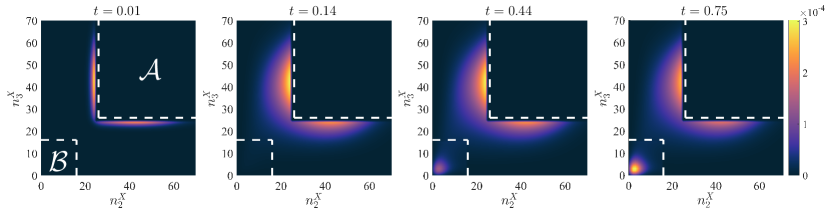
Notably, the time-evolved MPS state allows us to estimate the probability of any microstate of interest, even though it would be impossible to enumerate probabilities of all microstates. Alternatively, sets of microstates can be summed over to yield tractable marginal distributions. As an example, Fig. 4 shows the results of calculating for a 1D chain of Schlögl sites. Though there are three sites, site one is traced over to leave the two-dimensional joint probability of finding X molecules in site 2 and X molecules in site 3. At time zero, the distribution is initialized within region according to . As time progresses, a small flux of probability leaks from to . Because the overwhelming preference is to stay in , Fig. 4 highlights the rare transitions by only plotting the joint distribution outside of . Notice that, consistent with a steady-state approximation, while the population in gradually amasses, the distribution over microstates between and is nearly stationary. The slight asymmetry between sites is due to the fact that site 2 is in the bulk while site 3 lies on the boundary. The higher-dimensional joint has the anticipated symmetry under interchange of and . More generally, symmetry holds between interchanging sites and , as reflected in Fig. 6. In the next section, we illustrate the fact that the MPS state’s ability to capture the rare time-dependent flux is key to calculating the rate of traversing between basins.
V Many-body rate calculation
Having established the TDVP dynamics of an MPS state, we can now repeat the strategy of Eq. (7) to compute a transition rate between states and :
| (27) |
In doing so, there are a few important differences from Eq. (27). Most obviously, the TDVP dynamics includes the projection onto the MPS tangent space and must now be an MPS approximation to the steady-state distribution. Additionally, the meaning of and must be adapted to now define many-body analogs of the projectors onto the two metastable states. The single-voxel Schlögl model had an state defined as all microstates with occupancy above a threshold . Similarly, included all microstates with occupancy less than some other threshold . The -voxel Schlögl model generalizes to involve hypercubic metastable states with basins defined by and .
With these generalizations, the transition rate of Eq. (27) would measure the flux crossing into through its boundary, but if we are to compare with a transition path theory rate, we must exclude re-crossing events. In other words, we want to include trajectories which exit then some time later enter , but we want to exclude the flux that leaves and re-enters some time later without having returned to . When is sufficiently large, those re-crossings can be ignored, but when becomes small enough, those recrossings can become significant and must be removed. We note that the TDVP dynamics can just as well be executed with a modified absorbing-boundary-condition dynamics with effective Hamiltonian
| (28) |
where the reaction and diffusion Hamiltonians exclude events that exit . An explicit construction of that modified absorbing-boundary dynamics is provided in App. D, allowing us to directly remove the re-crossing events.
VI Numerical Evaluation of the -Voxel Schlögl Model Switching Rate
The formalism of the preceding sections has laid out a controllable approximation to extract rates between metastable states of RDMEs. Numerical experiments are necessary to evaluate whether that formalism can be practically useful. We set out to demonstrate that utility by computing the transition rates between high-occupancy and low-occupancy states of a -voxel Schlögl model as a function of . The model is parameterized by the four stochastic rate coefficients discussed in Sec. II. We sought rate coefficients that fall in a bistable regime, with sharp peaks of steady-state probability falling in high- and low-occupancy states. Since the dynamics would need to be truncated at some maximum occupancy , we furthermore wanted to limit how many molecules would naturally accrue in the high-occupancy state. By scanning parameters with the Schlögl model, we found parameters ( and ) compatable with an truncation and with a sharp bistability between and regions defined by the thresholds and . By linking multiple voxels together in a 1D chain with a diffusive hopping rate , it becomes rarer to switch between the two metastable states than it would be with a single isolated voxel. With multiple voxels, a switching event must flip the state of each voxel, and diffusion between neighboring voxels works to stabilize neighbors in identical high- or low-occupancy states. Due to that diffusive coupling between neighbors, the -voxel Schlögl model’s to transition is characterized by a correlated flip of all voxels, and the rarity of that correlated event depends on , the number of correlated voxels. It is therefore straightforward for us to push the rate-calculation methodologies into challenging regimes; can be decreased by growing .
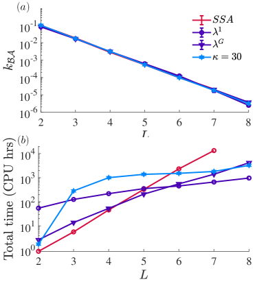
The most straightforward way to numerically detect the -dependence of the transition rate is via sampling of trajectories. Realizations of the continuous-time RDME, subject to the maximum voxel occupancy at fixed , were generated using the SSA. First, independent SSA realizations were initialized from a uniform distribution and propagated in parallel up to to approach the steady state distribution. Sampled configurations that fell within were then sampled as initial configurations for 400 independent trajectories which were evolved via the SSA until the trajectory first reached . From the trajectories, the transition rate was computed from the mean of those waiting times to reach : . Fig. 5a (red line) shows that the rate exponentially decreases as is increased, a result consistent with the exponential dependence of rate on volume in the well-mixed Schlögl model [74]. While the rate can be computed by trajectory sampling, the difficulty to do so (via brute force sampling) grows in proportion to the typical , meaning the computational cost grows exponentially with (see Fig. 5c).
The poor scaling of brute-force SSA sampled rate calculations has motivated so-called advanced sampling methods like FFS [10], which focus computational effort on the progress along a reaction coordinate. The idea is to introduce a reaction coordinate that resolves progress in transitioning from a value at the boundary of to at the boundary of . Rather than seek long trajectories that snake from all the way to , it can be beneficial to break the transition up into smaller trajectories that make some progress in moving to states with values of closer to than they started. This FFS scheme is particularly clever in that it can be statistically unbiased, meaning any choice of reaction coordinate (any mapping taking a microstate to a value of ) will yield the true rate in the infinite sampling limit. Despite that formal lack of bias, the computational cost of a FFS calculation depends strongly on the correlation between and the reaction’s progress [11]. If one already has a good idea of how the reactions rare transition events proceed, a smart can be constructed and the exponential scaling of the SSA can be avoided, but that identification of the reaction coordinate is seldom straightforward. For example, in the L-voxel Schlögl model, will to events typically be triggered by a high- to low-occupancy flip at a boundary voxel of the 1D chain or in the bulk? The boundary voxels have the benefit that they only have diffusion from one neighbor stabilizing the high-occupancy state, but the bulk voxels have the advantage of being more plentiful. In App. G we describe FFS calculations employing two reasonable choices of reaction coordinate. Those existing FFS methods can yield rates more cheaply than a brute force SSA calculation, but the speed up depends strongly on the reaction coordinate, the choice of which is nontrivial even for this simple model.
The DP/TDVP approach we have described offers a radically different strategy for circumventing the SSA scaling problem. Because the reaction-coordinate selection problem is hard, we developed the DP/TDVP strategy to bypass it entirely, computing the rate and reaction mechanism without prior information about how the transition events move through the high-dimensional state space. Fig. 5 shows that the reaction-coordinate-agnostic DP/TDVP approach indeed reproduces the SSA rates at lower computational expense, reducing the scaling from exponential to polynomial in . The SSA rate calculations can be made more accurate by collecting more trajectories, and the DP/TDVP calculations likewise offer a systematic way to improve accuracy in exchange for a greater computational expense. The two most prominent ways to adjust that accuracy are through the time step for the TDVP evolution and through the maximum bond dimension for the MPS state. In this work, a time step of was used throughout, and the trade-off between expense and accuracy was entirely tuned through the choice of . The single-site TDVP algorithm we used to propagate an MPS state does not alter the bond dimension of the MPS, so was entirely set by the bond dimension of the initial MPS. We therefore needed to approximate the steady state with different values of . Approximations were generated by starting with an initially uniform state using a bond dimension set to several different values between 5 and 30. Those uniform distributions were evolved with single-site TDVP for 10,000 time-steps allowing for the natural dynamics of to approach a stationary state with by time . Irreducibility of means the unique stationary state is the steady-state distribution . While would imply , does not guarantee that , only that the distribution is evolving very slowly. When transitions between and are slow, one can imagine reaching a local steady state distribution within and within but having probability very slowly repartitioning between the two. For our purposes, what matters is not that has exactly reached but rather that the distribution confined to , upon renormalization, has approached . Provided dynamics within is comparatively fast, this local steady state within is reached more rapidly than and is reasonably confirmed by checking that .
The renormalized distribution was then propagated under single-site TDVP with the absorbing-boundary dynamics (see App. D) for another 10,000 time steps, and projected onto to add up the total probability to have reached . Note that these 10,000 steps are not nearly enough to reach the steady state because the slow rate of transitioning from to is a bottleneck. As additional time steps of dynamics were taken, the growth of the transition flux from to was measured and plotted in Fig. 5b. That figure shows that at very short times (), the flux from to has not reached a steady state value because there hasn’t been enough time for any transitions. After that initial time , the plot plateaus at a value corresponding to the rate , a plateau that is reached orders of magnitude faster than the time for a typical SSA trajectory to make a transition. We find that if the bond dimension is insufficient (e.g., for in Fig. 5b), then the dynamics becomes unstable, reflected in erratic estimates for the conditional probability . As the bond dimension is grown (e.g., for in Fig. 5b), the estimates converge, allowing a stable rate to be extracted. That convergence as a function of is analyzed further in App. E. We find that setting the bond dimension to roughly 10 or 20 is often sufficient, but larger values of can only converge with a larger bond dimension. For example, Fig. 5a shows that SSA rates agree with calculations up to , but was required to push up to . Provided that larger bond dimension is used, the DP/TDVP rates reproduce the SSA rates across five orders of magnitude, up to and beyond the point that the brute-force SSA rates are practical.
Though the required bond dimension grows with , Fig. 5c shows that the expense to estimate the rate grows sub-exponentially. The blue and black dashed lines in that plot are the total number of CPU hours time to estimate the rate using TDVP with and respectively. Both SSA and TDVP were run using codes written in the Julia programming language [75] on equivalent CPUs with details of the runtime analysis described in App. F. While the required CPU hours, of course, depends on details of the hardware, parallelization, the particular implementation, we illustrate the difference in scaling when comparing identical implementations run in identical ways across different system sizes. Fig. 5c clearly demonstrates that difference in scaling between brute-force SSA and DP/TDVP. An increase in bond dimension increases the computation time, but it does not fundamentally alter the favorable scaling in . Comparison of computational expense with FFS is complicated by the fact that one can optimize FFS in many different ways (how many interfaces, which reaction coordinate, etc.), but App. G shows that the DP/TDVP calculations remain favorable even compared to FFS with a reasonable guess of an order parameter.
VII Deploying the tool
We have described a numerical tool to extract the rate of a rare switching event from a reaction-diffusion model, but the numerical value of that rate is often not the final goal. More than the value of the rate, it is desirable to know how the rate changes in response to controllable parameters. Fig. 5a showed one such variation—the switching rate falls off exponentially with the number of voxels . The essential physics of this exponential decay is consistent with a mechanism in which a boundary voxel of the 1D chain flips to create an interface between high- and low-occupation voxels. Subsequently, each voxel at the interface flips until the whole chain has flipped. Letting denote the small rate of flipping a boundary voxel and denote the small rate of flipping a voxel at the interface, it follows that at short times . If is the typical time to wait between interface flips, one therefore expects the exponential decay with .
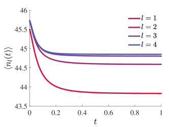
The rate calculations as a function of thus hint at a stepwise mechanism with a flipped voxel passing from one end of the chain to the other, but that mechanistic insight can also be more directly extracted from the DP/TDVP evolution. The time-evolution of contains information about the entire distribution that flows from to , and we can track the average number of molecules in each lattice site as a function of time. For example, Fig. 6 shows , the average number of molecules in voxel with ranging from 1 through 4 for an voxel lattice. At time , the plot shows the normalized steady-state confined to , the high-occupation-number state. In the steady state, the six bulk voxels, 2 through 7, have essentially indistinguishable mean occupancies, while the boundary voxels, 1 and 8, have slightly depressed means reflecting that it is marginally more likely for those two voxels to fluctuate to low-occupancy states. As the time is allowed to evolve for a timescale , the mean occupation of the boundary voxels drops markedly due to the influence of rare trajectories in which one or both boundary voxels can flip. Subsequent to that drop in , the mean occupancies of voxels 2 then 3 also drop, though less sharply, establishing the mechanistic sequence. After the molecular timescale , the rate of decrease in becomes linear, reflecting the steady-state flux from to .
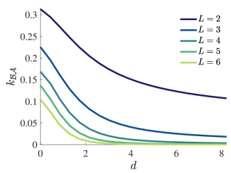
In addition to varying the extent of the space, it is interesting to tune the balance between reaction and diffusion events through the diffusive hopping rate . The sequential mechanism suggests that a limitation to the transition events emerges from , the probability of flipping the state of an interior voxel at an interface between low- and high-occupation states. The transition events thus have low- and high-occupation blocks separated by an interface that diffuses until the low-occupation block covers the entire system. When molecules diffuse between interface voxels, the interface itself can diffuse, and the faster the interface sweeps through the system, the faster the transition events. One might therefore anticipate that the flipping rate grows with . In fact, we find the exact opposite. Fig. 7 shows the results from varying the diffusion over 20 evenly spaced values while holding the bond-dimension fixed at . The rate decreases for each value of as is increased due to diffusion acting as an effective stabilizer of high-occupation states.
At , each voxel is an independent well-mixed system. The switching rate depends on the probability that each voxel independently experiences a collapse of population, dislodging it from its metastable high-occupation state. As grows, there is a diffusive mechanism to fight against that population collapse. When the population of a voxel wanders dangerously close to a tipping point, molecules could diffuse from a high-occupancy neighbor to restore the population. In the limit of very fast diffusion, the entire chain of voxels effectively behaves as a single large well-mixed system with a markedly lower switching rate because statistical fluctuations away from the metastable state get correspondingly smaller.
VIII Discussion
Using the 1D Schlögl model, we have demonstrated how TN calculations combined with the DP framework offer a new paradigm for numerical investigation of reaction-diffusion models, even when the physical bond dimension () is not small. That demonstration opens up a large class of RDME models which represent small well-mixed reactors, connected together by diffusive coupling. As illustrated in this work, these models can exhibit interesting physics when each reactor is small enough to exhibit significant statistical fluctuations and when the diffusion between reactors induces correlations between fluctuations in different reactors. In this work, our approach was to start with a well-studied kinetic toy model and to add spatial dynamics. Spatial extensions of other toy models like the Brusselator [76] or the Oregonator [77] would be amenable to similar numerical analysis because any reaction-diffusion model which can be written as a set of elementary reactions will have a DP representation. That representation can involve creation and annihilation operators for different particle types, not only for species X, but the mapping from reactions to effective Hamiltonians is systematic. Table 1 shows the effective Hamiltonians for several common (unchemostatted) reactions: unimolecular, bimolecular, and auto-catalytic. Given the set of reactions, it is comparatively straightforward to derive the DP representation, and computational tools already exist to generate an MPO [62] and propagate via TDVP from that DP form of the effective Hamiltonian.
| Reaction | Hamiltonian |
|---|---|
| \ceX -¿[] Y | |
| \ceX +Y -¿[] Z | |
| \ceX + Y -¿[] 2X |
As the TN techniques become increasingly well developed, one can imagine that the computational tools will offer generic “turn the crank” analysis of microscopic models of reaction-diffusion at the ensemble level. We anticipate these numerical approaches to be beneficial to both synthetic and biophysical reaction-diffusion systems. In the case of the former, the discretization of space into reactors can be explicitly realized, as in the microfluidic fabrication of a two-dimensional array of nanoliter-volume Belousov–Zhabotinsky (BZ) reactors [79]. In line with our 1D Schlögl model, the strength of coupling between those BZ nanoreactors is regulated by diffusion, and there is experimental interest in pattern formation as a function of that diffusive coupling. In the case of biophysics, sub-cellular dynamics is dominated by the generation and diffusion of proteins with small copy numbers. Much work has been devoted to understanding the logic of cellular decision making through stochastic CRN models, most famously gene regulatory models, which are most frequently studied in a well-mixed limit [80]. We see these TN tools as an intriguing pathway to numerically investigate the timescales and pathways for switching between metastable states in well-mixed CRNs like gene toggle switches [10] and in reaction-diffusion variants of those gene-regulatory models. Eventually, one can dream of bringing these methods to the broad array of systems biology applications where RDME models are widely simulated [81], including in large-scale GPU-accelerated simulations of systems with biologically-relevant size [82]. At present those sorts of reaction-diffusion model can only be numerically accessed through sampling approaches, and we expect the ensemble perspective will some day complement those efforts.
To move from the toy models to the synthetic and biophysical systems, it will be important to expand the ability of TNs to approximate correlation between species and voxels that are not simply connected through a 1D chain. Here, because our 1D chain of Schlögl reactors are connected only to their neighbors, it was natural to approximate the microscopic distribution with an MPS. That choice allowed us to capitalize on the efficient TDVP algorithm for MPS states, but a RDME with many dynamic species will not always be easily approximated by a 1D chain of tensors. If two chemical species are strongly correlated but far apart in the MPS structure, the MPS calculation will demand a very high bond dimension. It will be important for future work to dynamically adapt the bond dimension through subspace expansion [83] or by devising systematic ways to generate tractable TN architectures with connectivity mirroring the correlations between CRN species. Those technical advances may eventually lay the groundwork to move the methodology from this Schlögl study to the complex, biologically-motivated models where SSA realizations presently reign supreme.
IX Acknowledgments
We gratefully acknowledge Hadrien Vroylandt, Nils Strand, Geyao Gu, and Luis Pedro Garcia-Pintos for many insightful discussions. We are also grateful to Miles Stoudenmire, Matthew Fishman, Steven White, and other developers of ITensor, a library for implementing tensor network calculations, upon which this work was built. This research was supported in part through the computational resources and staff contributions provided for the Quest high performance computing facility at Northwestern University which is jointly supported by the Office of the Provost, the Office for Research, and Northwestern University Information Technology. The material presented in this manuscript is based upon work supported by the National Science Foundation under Grant No. 2141385. TRG is thankful that Phill Geissler could see this work in a preliminary form, but is deeply saddened that Phill’s much-too-soon passing prevented him from sharing more of his wisdom.
Appendix A Doi-Peliti encoding
Assume a set of elementary reactions are given. These can be encoded into a Doi-Peliti representation which converts each elementary reaction into a term of an effective Hamiltonian. The operator representations can then be exactly written as an MPO, as shown below. Consider an -site D lattice of well-mixed voxels. Inside each voxel the Schlögl model reactions can fire. A probability distribution will be written as a vector in the Fock space spanned by orthonormal basis vectors which correspond to single microstates, with occupancy of each voxel given by . For any two microstates and we thus have . Distributions over the microstates can be written as , where is the probability of microstate at time . When focusing on the voxel we will use the shorthand , where defines the state of the set of voxels that complement voxel . Each reaction of the Schlögl model contributes to the set of differential equations which describe the time evolution of . We must convert the local change in probability of microstate to the global action of the effective Hamiltonian on . The linear nature of the chemical master equation means we can consider one reaction at a time.
A.1 Reaction 1: \ceX + A -¿[~c_1] X
We start with the reaction . When this reaction fires inside site , the change in probability is
| (33) |
The first (positive) term captures the gain of probability into microstate from microstate . Two of the possible X molecules must come together to make the third, and there are total combinations. The second (negative) term of Eq. (33) accounts for the probability of already being in state at time . Notice that this reaction adds an X molecule, so if the system is already at the maximum cap of molecules, there can be no negative term at , to balance out conservation of probability. The loss term therefore requires extra care when there is an enforced cap since the loss term would come from a forbidden transition. Consequently, Eq. (33) can only apply to microstates whose voxel is not maximally occupied. For the general case, we could rewrite the evolution as
| (34) |
Summing each side of Eq. (34) over the Fock states yields
| (35) |
It is useful to match the argument of with the ket, which can be achieved by introducing the appropriate creation operator:
| (36) |
The term preceding the first ket is an operator, but all other terms preceding the kets are numbers that readily commute. We reorder those terms to get
| (37) |
Eqs. (12) give the identity , allowing both the gain and loss terms to be re-expressed in terms of powers of the creation and annihilation operators:
| (38) |
Notice that the creation and annihilation operators can now be factorized outside of the sum to yield two terms which look very similar to the Fock-space expansion .
| (39) |
The first term is like the expansion of except that the bounds of summation are shifted, including kets with occupancy through rather than through . The non-physical state with occupancy has no probability, so it can be excluded from the sum. Furthermore, the occupancy term can be added to the sum since . Consequently, the first sum of Eq. (39) is equivalent to . The second sum can also be expressed in terms of if we recognize that the delta function constraint can be viewed as the eigenvalue of a projector operator:
| (40) |
Hence, both sums of Eq. (39) simplify in terms of the same Fock state :
| (41) |
The factor of can be traced back to a combinatorial counting term for the unique number of ways to label the two X molecules that react. We absorb that counting term into the rate and extract from Eq. (41) the contribution to the effective Hamiltonian arising from the first reaction in site :
| (42) |
We take that direction of the reaction to be “forward” and use the superscript A because this is the reaction mediated by species A. By applying Eq. (17), the projector term can be rewritten in terms of a commutator of and to give an alternative form of expressed only in terms of the creation and annihilation operators, , and the maximal voxel occupancy :
| (43) |
This form, shows that in the limit Eq. 43 recovers the more standard bosonic result, . For compactness, we typically leave our expressions for contributions to the effective Hamiltonians as expressions that explicitly involve the finite-voxel projector, as in Eq. (42).
A.2 Reaction 2: \ceX -¿[~c_2] X + A
The reverse reaction, which transitions from an occupancy of to , has different ways to combine three of the X molecules together. Consequently, the change in probability for the reverse reaction is
| (44) |
Unlike the forward reaction, the negative term does not include a factor of that treats the maximal occupancy state differently than the others. The distinction is that the loss terms from reaction 2 arise when probability is lost from occupancy down to occupancy . Those loss terms are possible from through . If there are fewer than 3 molecules, the reaction 2 mechanism is not possible, but this restriction emerges naturally from the coefficients in Eq. (44). Expanding in the Fock basis therefore gives
| (45) |
Mirroring the treatment of the forward reaction, we rewrite the first using a lowering operator
| (46) |
Eqs. 12 imply and , which allow us to simplify Eq. (46) to
| (47) |
We recognize the second sum over as giving . The first sum ranges from through , but the term vanishes due to the occupancy cap. Furthermore, an term can be added to the sum since that term also vanishes (). Thus the first sum can be re-indexed to give . Performing both of those sums yields
| (48) |
The contribution to the effective Hamiltonian from the reverse A-mediated reaction in voxel is thus
| (49) |
where we have again absorbed the combinatorial term into . By summing together the forward and reverse reactions, we arrive at the effective Hamiltonian associated with the reversible -mediated reaction, quoted in Eq. (19):
| (50) |
A.3 Reaction 3: \ceB -¿[~c_3] X
Deriving the effective Hamiltonian for the third reaction is even more straightforward than the previous two. As in the first reaction, the loss term is only present if the microstate is not maximally occupied, so the probability for microstate evolves according to
| (51) |
In the Fock basis, this evolution becomes
| (52) |
We again seek to make the first ket’s microstate match the argument of by introducing the creation operator:
| (53) |
As in reaction 1, we re-index the first sum to get and we introduce the projector operator into the second sum to get , leaving
| (54) |
In this case, there is no combinatorial counting term, so and
| (55) |
A.4 Reaction 4: \ceX -¿[~c_4] B
The reverse reaction is like reaction 2 in that the reaction decreases X and therefore cannot cause an overflow beyond the maximal voxel occupancy. Consequently, the evolution of probability in microstate is
| (56) |
Expanding in the Fock space gives
| (57) |
As before, we expand into two sums. Upon checking the two boundary terms of the first sum, we re-index it and sum over microstates, recovering from both sums to get
| (58) |
The combinatorial term is again trivial, so , and
| (59) |
Combining Eqs. (55) and (59) yields the effective Hamiltonian arising from the reversible -mediated reaction, Eq. (20):
| (60) |
The diffusion operator of Eq. (21) is derived similarly by adding the maximal voxel occupancy constraint to the derivation of the bosonic diffusion operator [84].
Appendix B Matrix Product Operators
Notice that the terms contributing to the effective Hamiltonian (Eqs. (19), (20), and (21)) each take a “product” form in which the creation and annihilation operators at a site multiply other creation and annihilation operators at that same site or at a nearest-neighbor site. For systems with local and nearest-neighbor interactions, there exists a relatively simple representation of the effective Hamiltonian. Let be the local effective Hamiltonian of the reversible reactions occurring in voxel . The total effective Hamiltonian includes this local contribution summed over all voxels plus the . Owing to the nearest-neighbor interactions, these terms can be elegantly summed via a product of operator-valued vectors and matrices. We define the operator-valued vectors associated with voxels and as
| (61) |
and the operator-valued matrix associated with voxels through as
| (62) |
With these definitions, one can show that , with representing a contraction.
This decomposition of offers a highly efficient way to numerically encode the effective Hamiltonian as an MPO. While we have shown an explicit MPO decomposition for the nearest-neighbor situation, in practice one uses powerful automated packages such as AutoMPO in ITensor [65] to generate compressed forms of the MPO from the second-quantized expressions like Eqs. (19), (20), and (21).
Appendix C TDVP algorithm
As described in Sec. IV, we wish to approximate the evolution of the distribution:
| (63) |
by approximating as
| (64) |
Here is a distribution over microstates that can be expressed as an MPS using the (time-dependent) set of tensors . As in the main text, the distinct tensors are implicitly distinguished based on the labeling scheme for the physical index. Only a subset of possible distributions can be written in the form of , but as the bond dimension increases, that subset necessarily grows. We call these distributions which can be represented by MPS states the MPS manifold . Because generally evolves off , the Time-Dependent Variational Principle (TDVP) [67, 68] seeks the evolution of along the MPS manifold:
| (65) |
where is a projector mapping the infinitesimal change in probability onto the MPS manifold’s nearest (with respect to the norm) tangent vector. The projector in this equation of motion ensures that stays on for all times.
Remarkably, in the case of the MPS manifold, an explicit form for the projector can be written down as a sum of terms, of which have a correspondence to the tensors of the MPS and of which have a correspondence to the bonds. To write down that decomposition, it is beneficial to first define the environment tensors which were obliquely referenced in Sec. IV. Through gauge transformations, is expressed as
| (66) |
where the tensors are left-orthogonal and tensors are right-orthogonal, meaning
| (67) |
and
| (68) |
Summing the tensors found in Eq. (66) up to gives the left environment tensor
| (69) |
with physical indices counting the occupancy of sites through and a single uncontracted bond index . A similar sum over the indices of the tensors gives the right environment tensor
| (70) |
with physical indices counting the occupancy of sites through and a single uncontracted bond index .
In terms of the left and right environment tensor projectors,
| (71) |
and
| (72) |
we can now write out the terms of the projector for the MPS manifold [85, 72]:
| (73) |
The positive terms are associated to the tensors and the negative terms are associated to the bonds.
Integrating Eq. (65) for a time step gives
| (74) |
In the limit of an infinitesimal time step, we can factorize that exponential to act with one at a time. For example,
| (75) |
The operator has the physical interpretation of mapping site forward in time by a time step . To see this interpretation, we illustrate the action of on , where we assume the MPS has already be written in a mixed canonical form centered on site 2. The operator acts globally on the MPS state, but as long as is expressed in the mixed canonical form, only the tensor at site 2 will be altered. In that way, the term is implemented as a local update to a single tensor, a local update with the structure of a time evolution with a local effective Hamiltonian. The reduction from global to local operations is seen if the global exponential operator is expanded in a Taylor series:
| (76) |
Each term of the sum over can be expressed graphically, where the blue triangular MPS tensors indicate their left/right orthogonality by the direction they point toward the black diamond tensor at the center of the mixed canonical form:
![[Uncaptioned image]](/html/2301.03717/assets/x8.png)
By contracting over all of the tensors in the shaded purple region, we obtain the local tensor we call . Notice that the same tensor appears repeatedly in the higher order terms of the Taylor series. These terms can be re-summed to give back a local matrix exponential acting on site 2. Hence, by contracting (the black diamond) with we get .
Following the propagation, the newly updated tensor is then decomposed into two blocks via QR or SVD decomposition. Like how acted locally on the tensor at site 2, will act locally to propagate , but the interpretation is that the propagation is a time step backwards in time, owing to the negative sign in Eq. (73). is then contracted with the next tensor in the chain, , which is also still at time . In doing so, we shift gauge such that the new tensor assigned to site 2 is and the new center site tensor at site 3 becomes . Having shifted the center to site 3, one then iterates: acting with , performing another QR or SVD decomposition, acting with , shifting the gauge, then continuing to sweep down the line. Sweeping over the entire MPS from to evolves by .
Appendix D Modified Absorbing Boundary Condition Dynamics
To measure a rate from into without multiple crossings of ’s boundary, we define a modified dynamics via an effective Hamiltonian that zeroes out the rates of any reaction or diffusion event that would depart the region . Deriving the forms of and in Eq. (28) requires that we first identify the set of states and reactions that depart :
| (77) |
where is the complement of . For the Schögl model, only diffusion and the forward reactions can map out of . The states in are those where particles in the voxel are at the boundary to , and . The local boundary for in one voxel can be projected onto using . Combining with the projector , lets us define the projection operator
| (78) |
that maps onto states which are at the boundary in voxel but anywhere in in the other voxels. To build a projector that isolates all boundary configurations, we require that at least one voxel is on the boundary. We can build such a projector from the powerset expansion
| (79) |
where is the set of combinations from elements taken at a time.
For Eq. (79) becomes
Each product over at multiple voxels can be simplified noting that, which leads to
| (80) |
where the sum over is now all combinations of and where appears times. The advantage of Eq. (80) is that effective Hamiltonians can be projected onto only using local (single-voxel) projectors. In this work, consists of all molecule numbers less than . Then, projecting onto reactions that can map out of the effective Hamiltonians for the Schlögl model become
| (81) | ||||
| (82) |
Appendix E Error in TDVP rate calculations
When calculating observables using the ensemble method, sampling error is avoided, but there are several different sources for numerical error. Each source of error is controllable in that a parameter can be increased or decreased to systematically improve accuracy at the expense of a greater numerical cost. That trade-off between accuracy and cost is not straightforward, particularly because it can switch depending on which source of error dominates. The factorization of the time propagation in Eq. (75) relied upon a infinitesimal time step, but the computational expense grows essentially linearly with the number of timesteps 111We say essentially linearly rather than linearly because as time progresses the distribution can build richer correlations which can result in singular value decompositions that utilize the full bond dimension . Distributions with less rich correlations can be described by smaller tensors if the singular values are truncated at a threshold.. Consequently, one seeks a time step which is small enough but not too small. We highlight that the SSA has an effective time step that emerges naturally as the typical time between subsequent events, and that this time step shrinks as the system size grows. By contrast, the TDVP approach’s time step is a parameter one can choose irrespective of the system size. In addition to the time-step error, the propagation of the local tensors discussed in App C is implemented via a Krylov expansion. We found that 30 Krylov basis vectors were sufficient, but the model system here is not very sensitive to the number used. We have not presented a thorough analysis of time-step or Krylov errors because it is clear that our error is dominated by the bond dimension , which can severely limit the variational search space of allowable MPS distributions.
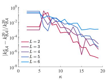
In order to get an estimate of how the bond dimension impacts the numerical errors, we repeated the TDVP rate for varying and . We would ideally compare each rate against an exact rate, but getting those exact rates is not numerically feasible for all system sizes considered. We have shown (see Fig. 5c) that for through , the bond dimension was sufficient to reproduce the SSA rates to within the size of the plot markers. For the purposes of analyzing the bond-dimension convergence, we thus take that calculation as the “converged” reference value and measure the approach to that value as increases from 2 to 20. Fig. 8 shows the absolute fractional error comparing the rate at a given bond-dimension and the reference rate, all with the same time step and Krylov dimension. We see that errors can already be very small at modest bond dimension (where the smaller tensors make the calculations substantially faster), and the errors shrink exponentially with growing for all values of .
Appendix F Runtime Analysis
Fig. 5c shows the total computational expense to estimate rates from the initial ensemble. The dominant purpose of communicating the number of CPU hours is to illustrate the scaling of computational expense with the system size. That is to say, the brute force SSA rates grow exponentially more costly as increases while the TDVP cost grows subexponentially. It is enticing to compare the costs to each other. At a fixed , was the SSA calculation or the TDVP calculation cheaper? Fig. 5c appears to answer that question, showing that the two methods have a cross-over with TDVP becoming cheaper for sufficiently large . We argue that the existence of the cross-over is a generic consequence of the different scalings with , but the exact location of the cross-over depends on specific details of the implementations of both SSA and TDVP. Considering the difference between the (black) and (blue) lines in Fig. 5c, one must be especially careful to compare one method versus the other. Each method has parameters that can be adjusted to improve accuracy, and to compare different CPU hour timings, one should have a sense that the two calculations are returning comparable accuracies. Even more importantly, one should recognize that although we have used the methods to compute the rate, the computational expense goes into two very different objects. In the case of SSA, that expense results in a collection of representative trajectories, while for TDVP it yields time-dependent joint distributions. If one were using the calculations to compute different quantities (say waiting time distributions rather than just the rate), the same TDVP joint distributions that were generated to compute the rates could be used at essentially no additional computational expense. By contrast, generating a converged waiting time distribution from SSA samples would require many more than the 400 trajectories used to estimate the rate. In a similar vein, in Fig. 6 we showed how the TDVP calculations give converged insight into the mechanism of the rare event, but the SSA approach would return only 400 representative events from which one would extrapolate.
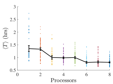
Having laid out the caveats, we spell out explicitly how we computed the total computational expense for these two classes of rate calculations (further information about forward flux sampling calculations follows in the next appendix). The TN calculations are not trivial to parallelize since the TDVP algorithm proceeds from one tensor to the next in serial, with the output of one tensor operation feeding into the next one. We did not seek a sophisticated parallelization, but we did note some imperfect parallelization could be easily accessed from the way the ITensor software in the Julia language handles the organization and contraction of tensors. Fig. 9 shows that this imperfect parallelization gave a roughly two-fold speed-up if 8 processors were used instead of a single processor. The computational expense reported in Fig. 5(c) is the total number of CPU hours for those 8 processors to complete the single-site TDVP dynamics with time step for 10,000 time steps with 30 Krylov dimensions starting from an already computed distribution in . In a sense, this timing is artificially worse than it would need to be. If we were willing to run for twice the duration of real time, we could decrease the total number of CPU hours for TDVP rates in Fig. 5(c) by a factor of 4 with a serial implementation.
Whereas the TDVP timing would have room for improvement with more sophisticated parallelization schemes, the SSA calculations are already fully optimized in that they are perfectly parallelizable. Each stochastic trajectory can and should be run on a separate CPU. The CPU hours reported in Fig. 5(c) is thus the sum of the wall times for 400 independent realizations, initialized in and run until was first reached. The cost for SSA calculations would shift up and down the log scale if one decided to use more or less than the 400 independent trajectories. Our choice here was to seek a number of trajectories that could make the SSA errorbars on the same order as the plot markers of Fig. 5(a).
Appendix G Comparison with Forward Flux Sampling
It is interesting to see how the computational expense of our rate calculation compares to advanced sampling rate calculations. Here we compare against the original FFS algorithm [10]. The key idea of FFS is that a (typically one-dimensional) progress coordinate is defined to decompose the single rare event from to down into less rare excursions that make partial progress along that order parameter. The progress coordinate is discretized to define a collection of non-overlapping interfaces . The FFS procedure decomposes the transition rate as
| (83) |
where is the flux to pass from to the interface and is the probability of reaching before first returning to conditioned upon initialization at the interface. To the extent that the chosen progress coordinate acts as a good reaction coordinate, the method can radically improve the efficiency of a rate calculation compared to brute force SSA, but if the order parameter is not “close enough” to the reaction coordinate, the conditional probability terms can become very expensive to compute [87]. It is tempting to think that requires a trajectory starting at and run until it hits either the next or the previous interface, but the actual procedure requires the trajectory to hit either the next interface or . When the progress coordinate poorly approximates the reaction coordinate, a tremendous amount of time can be wasted simulating trajectories slowly wandering back to from one of the final interfaces. The efficiency of FFS calculations additionally depends on the number of interfaces, their distance from each other, and the number of trajectories needed to resolve the conditional distributions. Given all the tunable knobs that go into a FFS rate calculation, it only makes sense to compare the numerical expense of TDVP rate calculations against a prudently designed FFS with a reasonable choice of progress coordinate.
Without a priori knowing the mechanism of the Schlögl reaction-diffusion switching events, we designed two different order parameters and performed calculations with both. For the first order parameter, we focus on the global number of X molecules, summed over all voxels. The interfaces for this order parameter measuring global progress are with . Remember that and , so this order parameter tracks the progress of the whole system in moving from less than molecules to more than molecules. The second order parameter, inspired by Fig. 6’s demonstration that the voxels on the end decrease first, uses only the number of molecules in the first voxel as the sign of progress. The interfaces for this order parameter measuring voxel 1 are with each interface recording the addition of another X molecule in voxel 1 (), so that and .
There are many ways to optimize both FFS calculations, for example, changing the number of interfaces, the number of trajectories to estimate , and the number of trajectories to estimate the conditional probabilities. These changes impact the computational expense, and it is not generally knowable how to tune those parameters to most cheaply decrease the errorbars of the rate calculation. We found that 4,000 trajectories were sufficient to get decent estimates of the flux for both order parameters, though the expense of computing that flux was much greater for than for . While the flux was more costly to compute for , the conditional probabilities were easier. Each conditional probability could be well estimated with only 4,000 additional trajectories per interface. Converging those conditional probability terms for required trajectories per interface, a cost that was at least partially offset by the cheaper calculation. For each order parameter we generated these samples to calculate ten independent estimates of the rate, allowing us to measure both the mean and standard error. From these standard errors, we determined that the FFS calculations were converged in line with the SSA errors in that plot.
A notable feature of FFS is that it will return the correct transition rates even when the order parameter is not a perfect reaction coordinate. Fig. 10a reflects that in that both and reproduce the rates given by the SSA and TDVP methods. However, the computational expense of the two are not identical. Fig. 10b plots the CPU hours needed to generate the samples that yield the means and standard errors of Fig. 10a. At small , is faster; at large , is faster. The FFS calculations have many tunable parameters. They could likely be improved through further refinement of order parameters, changing the number of interfaces, fine-tuning the number of samples for each conditional probability, etc. Still, we find it notable that our reasonable but perhaps unoptimized FFS implementations perform with similar (and slightly greater) expense as the TDVP rate calculations. This observation is particularly notable since the TDVP calculations do not need one to guess an order parameter and since they offer converged statistical information about the mechanism in addition to just giving the rate.
References
- Eyring [1935] H. Eyring, The activated complex in chemical reactions, The Journal of Chemical Physics 3, 107 (1935).
- Laidler and King [1983] K. J. Laidler and M. C. King, The development of transition-state theory, The Journal of Physical Chemistry 87, 2657 (1983).
- Truhlar and Garrett [1980] D. G. Truhlar and B. C. Garrett, Variational transition-state theory, Accounts of Chemical Research 13, 440 (1980).
- Grote and Hynes [1980] R. F. Grote and J. T. Hynes, The stable states picture of chemical reactions. II. Rate constants for condensed and gas phase reaction models, The Journal of Chemical Physics 73, 2715 (1980).
- Hynes [1985] J. T. Hynes, Chemical reaction dynamics in solution, Annual Review of Physical Chemistry 36, 573 (1985).
- Dellago et al. [1998] C. Dellago, P. G. Bolhuis, F. S. Csajka, and D. Chandler, Transition path sampling and the calculation of rate constants, The Journal of Chemical Physics 108, 1964 (1998).
- Bolhuis et al. [2002] P. G. Bolhuis, D. Chandler, C. Dellago, and P. L. Geissler, Transition path sampling: Throwing ropes over rough mountain passes, in the dark, Annual Review of Physical Chemistry 53, 291 (2002).
- Crooks and Chandler [2001] G. E. Crooks and D. Chandler, Efficient transition path sampling for nonequilibrium stochastic dynamics, Physical Review E 64, 026109 (2001).
- Gingrich and Geissler [2015] T. R. Gingrich and P. L. Geissler, Preserving correlations between trajectories for efficient path sampling, The Journal of Chemical Physics 142, 06B614_1 (2015).
- Allen et al. [2005] R. J. Allen, P. B. Warren, and P. R. ten Wolde, Sampling rare switching events in biochemical networks, Physical Review Letters 94, 018104 (2005).
- Allen et al. [2006] R. J. Allen, D. Frenkel, and P. R. ten Wolde, Simulating rare events in equilibrium or nonequilibrium stochastic systems, The Journal of Chemical Physics 124, 024102 (2006).
- Allen et al. [2009] R. J. Allen, C. Valeriani, and P. R. ten Wolde, Forward flux sampling for rare event simulations, Journal of Physics: Condensed Matter 21, 463102 (2009).
- Ma and Dinner [2005] A. Ma and A. R. Dinner, Automatic method for identifying reaction coordinates in complex systems, The Journal of Physical Chemistry B 109, 6769 (2005).
- Isaacson and Peskin [2006] S. A. Isaacson and C. S. Peskin, Incorporating diffusion in complex geometries into stochastic chemical kinetics simulations, SIAM Journal on Scientific Computing 28, 47 (2006).
- Erban et al. [2007] R. Erban, J. Chapman, and P. Maini, A practical guide to stochastic simulations of reaction-diffusion processes, arXiv preprint arXiv:0704.1908 10.48550/arXiv.0704.1908 (2007).
- Fange et al. [2010] D. Fange, O. G. Berg, P. Sjöberg, and J. Elf, Stochastic reaction-diffusion kinetics in the microscopic limit, Proceedings of the National Academy of Sciences 107, 19820 (2010).
- Wilkinson [2018] D. J. Wilkinson, Stochastic modelling for systems biology (CRC press, 2018).
- Smith and Grima [2019] S. Smith and R. Grima, Spatial stochastic intracellular kinetics: A review of modelling approaches, Bulletin of Mathematical Biology 81, 2960 (2019).
- Craciun et al. [2006] G. Craciun, Y. Tang, and M. Feinberg, Understanding bistability in complex enzyme-driven reaction networks, Proceedings of the National Academy of Sciences 103, 8697 (2006).
- Krause et al. [2021] A. L. Krause, E. A. Gaffney, P. K. Maini, and V. Klika, Modern perspectives on near-equilibrium analysis of Turing systems, Philosophical Transactions of the Royal Society A 379, 20200268 (2021).
- Kondo and Miura [2010] S. Kondo and T. Miura, Reaction-diffusion model as a framework for understanding biological pattern formation, Science 329, 1616 (2010).
- Turing [1952] A. Turing, The chemical basis of morphogenesis. philosophical transactions of the royal society, Philosophical Transactions of the Royal Society of London B 237, 37 (1952).
- Cross and Hohenberg [1993] M. C. Cross and P. C. Hohenberg, Pattern formation outside of equilibrium, Reviews of Modern Physics 65, 851 (1993).
- McQuarrie [1967] D. A. McQuarrie, Stochastic approach to chemical kinetics, Journal of Applied Probability 4, 413 (1967).
- Lee DeVille et al. [2006] R. E. Lee DeVille, C. B. Muratov, and E. Vanden-Eijnden, Non-meanfield deterministic limits in chemical reaction kinetics, The Journal of Chemical Physics 124, 231102 (2006).
- McAdams and Arkin [1997] H. H. McAdams and A. Arkin, Stochastic mechanisms in gene expression, Proceedings of the National Academy of Sciences 94, 814 (1997).
- Thattai and Van Oudenaarden [2001] M. Thattai and A. Van Oudenaarden, Intrinsic noise in gene regulatory networks, Proceedings of the National Academy of Sciences 98, 8614 (2001).
- Vilar et al. [2002] J. M. Vilar, H. Y. Kueh, N. Barkai, and S. Leibler, Mechanisms of noise-resistance in genetic oscillators, Proceedings of the National Academy of Sciences 99, 5988 (2002).
- Paulsson [2004] J. Paulsson, Summing up the noise in gene networks, Nature 427, 415 (2004).
- Tian and Burrage [2006] T. Tian and K. Burrage, Stochastic models for regulatory networks of the genetic toggle switch, Proceedings of the national Academy of Sciences 103, 8372 (2006).
- Heuett and Qian [2006] W. J. Heuett and H. Qian, Grand canonical Markov model: a stochastic theory for open nonequilibrium biochemical networks, The Journal of Chemical Physics 124, 044110 (2006).
- Gillespie et al. [2013] D. T. Gillespie, A. Hellander, and L. R. Petzold, Perspective: Stochastic algorithms for chemical kinetics, The Journal of Chemical Physics 138, 05B201_1 (2013).
- Yang et al. [2006] C. Yang, D. T. Gillespie, and L. R. Petzold, Efficient step size selection for the tau-leaping simulation method, The Journal of Chemical Physics 124, 044109 (2006).
- Munsky and Khammash [2006] B. Munsky and M. Khammash, The finite state projection algorithm for the solution of the chemical master equation, The Journal of Chemical Physics 124, 044104 (2006).
- Kazeev et al. [2014] V. Kazeev, M. Khammash, M. Nip, and C. Schwab, Direct solution of the chemical master equation using quantized tensor trains, PLoS Computational Biology 10, e1003359 (2014).
- Vo and Sidje [2017] H. D. Vo and R. B. Sidje, An adaptive solution to the chemical master equation using tensors, The Journal of Chemical Physics 147, 044102 (2017).
- Helms et al. [2019] P. Helms, U. Ushnish, and G. K.-L. Chan, Dynamical phase behavior of the single-and multi-lane asymmetric simple exclusion process via matrix product states, Physical Review E 100, 022101 (2019).
- Strand et al. [2022a] N. E. Strand, H. Vroylandt, and T. R. Gingrich, Using tensor network states for multi-particle Brownian ratchets, The Journal of Chemical Physics 156, 221103 (2022a).
- Strand et al. [2022b] N. E. Strand, H. Vroylandt, and T. R. Gingrich, Computing time-periodic steady-state currents via the time evolution of tensor network states, The Journal of Chemical Physics 157, 054104 (2022b).
- Schlögl [1972] F. Schlögl, Chemical reaction models for non-equilibrium phase transitions, Zeitschrift für Physik 253, 147 (1972).
- Kim et al. [2017] C. Kim, A. Nonaka, J. B. Bell, A. L. Garcia, and A. Donev, Stochastic simulation of reaction-diffusion systems: A fluctuating-hydrodynamics approach, The Journal of Chemical Physics 146, 124110 (2017).
- Vellela and Qian [2009] M. Vellela and H. Qian, Stochastic dynamics and non-equilibrium thermodynamics of a bistable chemical system: the Schlögl model revisited, Journal of The Royal Society Interface 6, 925 (2009).
- Nicholson et al. [2018] S. B. Nicholson, J. S. Greenberg, and J. R. Green, Entrance and escape dynamics for the typical set, Physical Review E 97, 012146 (2018).
- Higham [2008] D. J. Higham, Modeling and simulating chemical reactions, SIAM Review 50, 347 (2008).
- Nicolis and Turner [1977] G. Nicolis and J. W. Turner, Stochastic analysis of a nonequilibrium phase transition: Some exact results, Physica A: Statistical Mechanics and its Applications 89, 326 (1977).
- Roux [2022] B. Roux, Transition rate theory, spectral analysis, and reactive paths, The Journal of Chemical Physics 156, 134111 (2022).
- E and Vanden-Eijnden [2010] W. E and E. Vanden-Eijnden, Transition-path theory and path-finding algorithms for the study of rare events., Annual Review of Physical Chemistry 61, 391 (2010).
- Ohkubo [2013] J. Ohkubo, Algebraic probability, classical stochastic processes, and counting statistics, Journal of the Physical Society of Japan 82, 084001 (2013).
- Täuber [2014] U. C. Täuber, Critical dynamics: A field theory approach to equilibrium and non-equilibrium scaling behavior (Cambridge University Press, 2014).
- Doi [1976] M. Doi, Stochastic theory of diffusion-controlled reaction, Journal of Physics A: Mathematical and General 9, 1479 (1976).
- Peliti [1985] L. Peliti, Path integral approach to birth-death processes on a lattice, Journal de Physique 46, 1469 (1985).
- Rey and Cardy [1999] P. Rey and J. Cardy, Asymptotic form of the approach to equilibrium in reversible recombination reactions, Journal of Physics A: Mathematical and General 32, 1585 (1999).
- Reyes-Velázquez et al. [2023] A. Reyes-Velázquez, A. Molgado, J. Berra-Montiel, and J. A. Martinez-Gonzalez, A general path–integral Monte Carlo method for exact simulations of chemical reaction networks, The Journal of Physical Chemistry A 127, 4363 (2023).
- Vastola [2021] J. J. Vastola, Solving the chemical master equation for monomolecular reaction systems and beyond: a Doi-Peliti path integral view, Journal of Mathematical Biology 83, 48 (2021).
- Yang et al. [2017] X. Yang, P. Liu, and J. Zhang, Analytical time-dependent distributions for two common signaling systems, Chinese Journal of Physics 55, 289 (2017).
- Harsh and Sollich [2023] M. Harsh and P. Sollich, Accurate dynamics from self-consistent memory in stochastic chemical reactions with small copy numbers, arXiv preprint arXiv:2303.00029 10.48550/arXiv.2303.00029 (2023).
- Garrahan et al. [2007] J. P. Garrahan, R. L. Jack, V. Lecomte, E. Pitard, K. van Duijvendijk, and F. van Wijland, Dynamical first-order phase transition in kinetically constrained models of glasses, Physical Review Letters 98, 195702 (2007).
- Garrahan et al. [2009] J. P. Garrahan, R. L. Jack, V. Lecomte, E. Pitard, K. van Duijvendijk, and F. van Wijland, First-order dynamical phase transition in models of glasses: an approach based on ensembles of histories, Journal of Physics A: Mathematical and Theoretical 42, 075007 (2009).
- Lan et al. [2006] Y. Lan, W. ans P. G Wolynes, and G. A. Papoian, A variational approach to the stochastic aspects of cellular signal transduction, The Journal of Chemical Physics 125, 124106 (2006).
- Giuli and Scalliet [2022] E. D. Giuli and C. Scalliet, Dynamical mean-field theory: from ecosystems to reaction networks, Journal of Physics A: Mathematical and Theoretical 55, 474002 (2022).
- Bothe and Pruessner [2021] M. Bothe and G. Pruessner, Doi-Peliti field theory of free active Ornstein-Uhlenbeck particles, Physical Review E 103, 062105 (2021).
- Schollwöck [2011] U. Schollwöck, The density-matrix renormalization group in the age of matrix product states, Annals of Physics 326, 96 (2011).
- Causer et al. [2022] L. Causer, M. C. Bañuls, and J. P. Garrahan, Finite time large deviations via matrix product states, Physical Review Letters 128, 090605 (2022).
- del Razo et al. [2022] M. J. del Razo, D. Frömberg, A. V. Straube, C. Schütte, F. Höfling, and S. Winkelmann, A probabilistic framework for particle-based reaction–diffusion dynamics using classical fock space representations, Letters in Mathematical Physics 112, 1 (2022).
- Fishman et al. [2022] M. Fishman, S. R. White, and E. M. Stoudenmire, The ITensor Software Library for Tensor Network Calculations, SciPost Phys. Codebases , 4 (2022).
- Orús [2014] R. Orús, A practical introduction to tensor networks: Matrix product states and projected entangled pair states, Annals of Physics 349, 117 (2014).
- Dirac [1930] P. A. Dirac, Note on exchange phenomena in the Thomas atom, in Mathematical Proceedings of the Cambridge Philosophical Society, Vol. 26 (Cambridge University Press, 1930) pp. 376–385.
- Haegeman et al. [2011] J. Haegeman, J. I. Cirac, T. J. Osborne, I. Pižorn, H. Verschelde, and F. Verstraete, Time-dependent variational principle for quantum lattices, Physical Review Letters 107, 070601 (2011).
- Vanderstraeten et al. [2019] L. Vanderstraeten, J. Haegeman, and F. Verstraete, Tangent-space methods for uniform matrix product states, SciPost Physics Lecture Notes , 007 (2019).
- Paeckel et al. [2019] S. Paeckel, T. Köhler, A. Swoboda, S. R. Manmana, U. Schollwöck, and C. Hubig, Time-evolution methods for matrix-product states, Annals of Physics 411, 167998 (2019).
- Haegeman et al. [2016] J. Haegeman, C. Lubich, I. Oseledets, B. Vandereycken, and F. Verstraete, Unifying time evolution and optimization with matrix product states, Physical Review B 94, 165116 (2016).
- Lubich et al. [2015] C. Lubich, I. V. Oseledets, and B. Vandereycken, Time integration of tensor trains, SIAM Journal on Numerical Analysis 53, 917 (2015).
- Vidal [2003] G. Vidal, Efficient classical simulation of slightly entangled quantum computations, Physical Review Letters 91, 147902 (2003).
- Vlysidis and Kaznessis [2018] M. Vlysidis and Y. N. Kaznessis, On differences between deterministic and stochastic models of chemical reactions: Schlögl solved with ZI-closure, Entropy 20, 678 (2018).
- Bezanson et al. [2017] J. Bezanson, A. Edelman, S. Karpinski, and V. B. Shah, Julia: A fresh approach to numerical computing, SIAM Review 59, 65 (2017).
- Tyson [1973] J. J. Tyson, Some further studies of nonlinear oscillations in chemical systems, The Journal of Chemical Physics 58, 3919 (1973).
- Field and Noyes [1974] R. J. Field and R. M. Noyes, Oscillations in chemical systems. IV. Limit cycle behavior in a model of a real chemical reaction, The Journal of Chemical Physics 60, 1877 (1974).
- Schulz and Reineker [2005] M. Schulz and P. Reineker, Exact substitute processes for diffusion–reaction systems with local complete exclusion rules, New Journal of Physics 7, 31 (2005).
- Litschel et al. [2018] T. Litschel, M. M. Norton, V. Tserunyan, and S. Fraden, Engineering reaction–diffusion networks with properties of neural tissue, Lab on a Chip 18, 714 (2018).
- Warren and ten Wolde [2004] P. B. Warren and P. R. ten Wolde, Enhancement of the stability of genetic switches by overlapping upstream regulatory domains, Physical Review Letters 92, 128101 (2004).
- Wilkinson [2009] D. J. Wilkinson, Stochastic modelling for quantitative description of heterogeneous biological systems, Nature Reviews Genetics 10, 122 (2009).
- Hallock et al. [2014] M. J. Hallock, J. E. Stone, E. Roberts, C. Fry, and Z. Luthey-Schulten, Simulation of reaction diffusion processes over biologically relevant size and time scales using multi-GPU workstations, Parallel Computing 40, 86 (2014).
- Hubig et al. [2015] C. Hubig, I. P. McCulloch, U. Schollwöck, and F. A. Wolf, Strictly single-site DMRG algorithm with subspace expansion, Physical Review B 91, 155115 (2015).
- Cardy [2006] J. Cardy, Reaction-diffusion processes (2006).
- Haegeman et al. [2013] J. Haegeman, T. J. Osborne, and F. Verstraete, Post-matrix product state methods: To tangent space and beyond, Physical Review B 88, 075133 (2013).
- Note [1] We say essentially linearly rather than linearly because as time progresses the distribution can build richer correlations which can result in singular value decompositions that utilize the full bond dimension . Distributions with less rich correlations can be described by smaller tensors if the singular values are truncated at a threshold.
- Hussain and Haji-Akbari [2020] S. Hussain and A. Haji-Akbari, Studying rare events using forward-flux sampling: Recent breakthroughs and future outlook, The Journal of Chemical Physics 152, 060901 (2020).