The distribution of the number of cycles
in directed and undirected random 2-regular graphs

Abstract

We present analytical results for the distribution of the number of cycles in directed and undirected random 2-regular graphs (2-RRGs) consisting of $N$ nodes. In directed 2-RRGs each node has one inbound link and one outbound link, while in undirected 2-RRGs each node has two undirected links. Since all the nodes are of degree $k=2$, the resulting networks consist of cycles. These cycles exhibit a broad spectrum of lengths, where the average length of the shortest cycle in a random network instance scales with $\ln N$, while the length of the longest cycle scales with $N$. The number of cycles varies between different network instances in the ensemble, where the mean number of cycles $\langle S\rangle$ scales with $\ln N$. Here we present exact analytical results for the distribution $P_{N}(S=s)$ of the number of cycles $s$ in ensembles of directed and undirected 2-RRGs, expressed in terms of the Stirling numbers of the first kind. In both cases the distributions converge to a Poisson distribution in the large $N$ limit. The moments and cumulants of $P_{N}(S=s)$ are also calculated. The statistical properties of directed 2-RRGs are equivalent to the combinatorics of cycles in random permutations of $N$ objects. In this context our results recover and extend known results. In contrast, the statistical properties of cycles in undirected 2-RRGs have not been studied before.

I Introduction

Random networks (or graphs) consist of a set of $N$ nodes that are connected to each other by edges in a way that is determined by some random process. They provide a useful conceptual framework for the study of a large variety of systems and processes in science, technology and society [1, 2, 3, 4, 5, 8, 6, 7, 9]. The structure of a random network can be characterized by the degree distribution $P(k)$. Here we focus on a special class of random networks, called random regular graphs (RRGs), which exhibit degenerate degree distributions of the form

$$P(k)=\delta_{k,c},$$ (1)

where $\delta_{k,k^{\prime}}$ is the Kronecker delta and $c\geq 1$ is an integer. While the degrees of all the nodes in these networks are the same, their connectivity is random and uncorrelated. In that sense, the RRG is a special case of the class of configuration model networks, which exhibit a specified degree distribution $P(k)$, but no degree-degree correlations [10, 11, 12, 13]. While RRGs with $c=1$ consist of isolated dimers, RRGs with $c\geq 3$ form a giant component. Thus, RRGs with $c=2$ are a marginal case, separating between the subcritical regime of $c<2$ and supercritical regime of $c>2$. Note that unlike some other configuration model networks that exhibit a coexistence of a giant component and finite tree components above the percolation transition, in RRGs with $c\geq 3$ the giant component encompasses the whole network.

RRGs with $c=2$, referred to as random 2-regular graphs (2-RRGs), consist of isolated cycles of various lengths. The lengths of these cycles are not determined by the topology, but by entropic considerations. An important distinction is between directed 2-RRGs, in which each node has one inbound link and one outbound link, and undirected 2-RRGs, in which each node has two undirected links. In both cases the cycles can be considered as isolated components of the network, where the length of each cycle is equal to the size of the network component that consists of this cycle.

In this paper we present exact analytical results for the distribution of the number of cycles in ensembles of directed and undirected 2-RRGs that consist of $N$ nodes. The results are expressed in terms of the Stirling numbers of the first kind. We first calculate the joint probability distribution of cycle lengths. This is done by mapping the directed and undirected 2-RRGs into combinatorically equivalent permutation problems. From the joint distribution of cycle lengths we extract the distribution $P_{N}(S=s)$ of the number of cycles in random instances of directed and undirected 2-RRGs. In both cases $P_{N}(S=s)$ converges to a Poisson distribution in the large $N$ limit. The moments and cumulants of $P_{N}(S=s)$ are also calculated. The similarities and differences between the results obtained for the directed and undirected 2-RRGs are discussed. The statistical properties of directed 2-RRGs are equivalent to the combinatorics of cycles in random permutations of $N$ objects. In this context our results recover and extend known results. In contrast, the statistical properties of cycles in undirected 2-RRGs have not been studied before. The results presented in this paper are derived specifically for $c=2$ and do not apply to the more general case of RRGs with $c\geq 3$.

The paper is organized as follows. In Sec. II we present the directed and undirected 2-RRGs. The joint distributions of cycle lengths are presented in Sec. III. In Sec. IV we calculate the distribution $P_{N}(S=s)$ of the number of cycles. In Sec. V we calculate the moments and cumulants of $P_{N}(S=s)$. The results are discussed in Sec. VI and summarized in Sec. VII.

II Random 2-regular graphs

In both directed and undirected 2-RRGs, each node has two links and the resulting network consists of a set of cycles. In the directed case each node has one inbound link and one outbound link, while in the undirected case each node has two undirected links. Below we briefly present the properties of directed and undirected 2-RRGs and their construction.

II.1 Directed 2-RRGs

To construct a directed 2-RRG one first assembles $N$ nodes such that each node has one inbound stub and one outbound stub. During the network construction process, at each time step one picks a random outbound stub and a random inbound stub among the remaining open stubs and connects them to each other. This process is repeated $N$ times, until no open stubs remain. This procedure follows the standard construction process of directed configuration model networks, in which pairs of outbound and inbound stubs rather than pairs of nodes are selected for connection. The resulting ensemble of networks obtained from this procedure is referred to as stub-labeled graphs [14]. During the construction process, directed chains of nodes of different lengths are formed. In case that the open outbound stub of one chain is selected to connect to the open inbound stub of another chain, they are connected and form a longer chain. In case that the outbound and the inbound stubs at both ends of the same chain are selected, their connection closes the chain and turns it into a cycle. Once a chain of nodes becomes a cycle it does not connect to other nodes and its structure remains unchanged. At the end of the construction, the whole network consists of cycles of different lengths.

In Fig. 1(a) we present a single instance of a directed 2-RRG of $N=14$ nodes, which consists of cycles of lengths $s=1,2,3,3$ and $5$. In the 2-RRGs considered here we allow the outbound and inbound stubs of the same node to be connected to each other. In such case, one obtains a self-loop of length $\ell=1$. We also allow the connection of a pair of outbound and inbound stubs, which belong to nodes that are already connected. In such case, the resulting cycle is of length $\ell=2$. This choice simplifies the analysis.

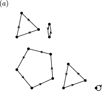
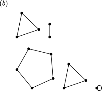
Figure 1: Illustration of a single instance of a 2-RRG of $N=14$ nodes, which consists of cycles of lengths $s=1,2,3,3$ and $5$, in the directed case (a) and in the undirected case (b).

Consider a directed 2-RRG consisting of $N$ distinguishable nodes, which are marked by the labels $i=1,2,\dots,N$. In the construction of such a network the first selected inbound stub has $N$ possible outbound stubs to which it may connect. The second selected inbound stub has only $N-1$ outbound stubs to which it may connect. Continuing this process we conclude that there are $N!$ possible ways to connect the $N$ nodes. In fact, the combinatorics of directed 2-RRGs consisting of $N$ nodes is equivalent to the permutation problem of $N$ objects [16, 15, 17]. This permutation problem can be described by a line of $N$ cells labeled by $i=1,2,\dots,N$, and a corresponding set of $N$ labeled balls. The number of ways to distribute the balls between the cells, one ball in each cell, is

$$R_{\rm D}=N!,$$ (2)

where each arrangement of the balls in the cells corresponds to a specific network instance. In this representation, a ball $i^{\prime}$ located in cell $i$ represents a directed link from $i$ to $i^{\prime}$. Similarly, a ball $i^{\prime\prime}$ located in cell $i^{\prime}$ represents a directed link from $i^{\prime}$ to $i^{\prime\prime}$. One can follow these directed links until the cell in which ball $i$ resides is reached and the cycle is closed. Repeating this process for all the balls and cells provides the structure of cycles associated with the specific permutation. The length of each cycle is given by the number of balls included in the cycle.

The statistical properties of cycles in random permutations of $N$ objects have been studied extensively [18, 20, 19]. In particular, the properties of the longest cycle in each permutation received much attention. It was found that the expectation value of the length of the longest cycle in a random permutation of $N$ objects is equal to $\lambda N$, where $\lambda=0.6243...$ is the Golomb-Dickman constant [21, 23, 22]. Interestingly, this constant plays a role in the prime factorization of a random integer. More specifically, it was found that the asymptotic average number of digits in the largest prime factor of a random $N$-digit number is $\lambda N$ [21, 24, 22]. In the other extreme, the average length of the shortest cycle in a random permutation of $N$ objects was also calculated and was found to be $e^{-\gamma}\ln N$, where $\gamma=0.5772...$ is the Euler-Mascheroni constant [16, 22].

II.2 Undirected 2-RRGs

To construct an undirected 2-RRG one first assembles $N$ nodes such that each node is connected to two undirected stubs. At each time step one selects a random pair of stubs among the remaining open stubs and connects them to each other. This process is repeated $N$ times, until no open stubs remain. This procedure follows the standard construction process of undirected configuration model networks, in which pairs of stubs rather than pairs of nodes are selected for connection [10, 11, 12, 13]. The resulting ensemble of networks obtained from this procedure is referred to as stub-labeled graphs [14]. Initially, one obtains linear chains of nodes of increasing lengths that eventually close and form cycles. Here we consider undirected 2-RRGs in which we allow the two stubs of the same node to be connected to each other and form a self-loop of length $\ell=1$. We also allow the connection of a pair of stubs which belong to nodes that are already connected, resulting in a cycle of length $\ell=2$. In Fig. 1(b) we present a single instance of an undirected 2-RRG of $N=14$ nodes, which consist of cycles of lengths $s=1,2,3,3$ and $5$.

Consider an ensemble of undirected 2-RRGs consisting of $N$ nodes. In the construction of such network the first selected stub has $2N-1$ other stubs to which it may connect. The second selected stub has $2N-3$ other stubs to which it may connect. Continuing this process we conclude that there are

$$R_{\rm U}=(2N-1)!!.$$ (3)

possible ways to construct such network, where $m!!$ is the double factorial of $m$. The statistical properties of the resulting ensemble of networks can be mapped to the combinatorial problem described below. Consider a set of $2N$ balls, such that for each value of $i=1,2,\dots,N$ there are two identical balls on which the label $i$ is marked. The two balls labeled by a given value of $i$ represent the two stubs of node $i$. In addition, there are $N$ unlabeled boxes such that in each box there is room for two balls. The $2N$ balls are then distributed uniformly at random in the $N$ boxes, where each box contains two balls. Each pair of balls that resides in the same box represents one edge of the network. For example, if a ball labeled by $i$ and a ball labeled by $i^{\prime}$ are in the same box, it means that there is an edge between the nodes $i$ and $i^{\prime}$. Similarly, if the other ball labeled by $i^{\prime}$ is in the same box with a ball labeled $i^{\prime\prime}$, it means that there is an edge between the nodes $i^{\prime}$ and $i^{\prime\prime}$. One can follow this chain until reaching the box in which the second ball labeled by $i$ resides, thus closing the cycle. The number of possible ways to distribute the $2N$ balls in the $N$ cells is given by

$$R_{\rm U}=\frac{(2N)!}{2^{N}N!},$$ (4)

where the numerator accounts for the number of permutations of $2N$ balls, the $N!$ term in the denominator accounts for the number of permutations of the $N$ identical cells, and the term $2^{N}$ accounts for the fact that the order in which the two balls are placed in each cell is unimportant. Note that $(2N)!=(2N-1)!!(2N)!!$ and $2^{N}N!=(2N)!!$. These two identities establish the equivalence between Eqs. (3) and (4).

III The joint distribution of cycle lengths

Both versions of the 2-RRG, with directed and undirected links, consist of closed cycles of different lengths. The configuration of cycles in a given network instance can be described by the sequence of cycle lengths, $\ell_{1},\ell_{2},\dots,\ell_{s}$, where $1\leq\ell_{i}\leq N$, $s$ is the number of cycles in the given network instance and

$$\sum_{i=1}^{s}\ell_{i}=N.$$ (5)

For convenience and uniqueness, we order the lengths in increasing order, such that $\ell_{1}\leq\ell_{2}\leq\dots\leq\ell_{s}$.

Another way to describe the configuration of cycles in a given network instance is in the form $\{g_{\ell}\}_{\ell=1}^{N}=\{g_{1},g_{2},\dots,g_{N}\}$, where $g_{\ell}$ is the number of cycles of length $\ell$. The $g_{\ell}$’s satisfy the condition

$$\sum_{\ell=1}^{N}\ell g_{\ell}=N,$$ (6)

which is equivalent to Eq. (5). The number of cycles in such a network instance can be expressed by

$$s=\sum_{\ell=1}^{N}g_{\ell}.$$ (7)

The joint distribution of cycle lengths in an ensemble of 2-RRGs consisting of $N$ nodes is denoted by $P_{N}(\{G_{\ell}\}=\{g_{\ell}\})$, under the condition of Eq. (6). For convenience we use the notation $P_{N}(\{g_{\ell}\})$. Below we consider the joint distributions of the cycle lengths in directed and undirected 2-RRGs.

III.1 Joint distribution of cycle lengths in directed 2-RRGs

Consider an ensemble of directed 2-RRGs that consist of $N$ nodes. The number of configurations of the form $\{g_{\ell}\}$ is given by

$$N(\{g_{\ell}\})=N!\prod_{\ell=1}^{N}\frac{1}{{\ell}^{g_{\ell}}g_{\ell}!}\delta_{\sum\ell g_{\ell},N}.$$ (8)

To understand the first term in the denominator, consider a cycle of length $\ell$. Such cycle exhibits $\ell$ cyclic permutations. This yields the first term in the denominator, which is raised to the power $g_{\ell}$ to account for the number of cycles of length $\ell$. The term $g_{\ell}!$ accounts for the permutations between the $g_{\ell}$ degenerate cycles of length $\ell$, which correspond to the same configuration, while the Kronecker delta imposes the condition of Eq. (6). Dividing the number of configurations $N(\{g_{\ell}\})$ by the total number of configurations $R_{D}$, given by Eq. (2), we obtain the joint probability distribution of cycle lengths. It is given by

$$P_{N}(\{g_{\ell}\})=\prod_{\ell=1}^{N}\frac{1}{{\ell}^{g_{\ell}}g_{\ell}!}\delta_{\sum\ell g_{\ell},N}.$$ (9)

It can be shown that this probability distribution is normalized, namely

$$\sum_{g_{1}}\sum_{g_{2}}\dots\sum_{g_{N}}P_{N}(\{g_{\ell}\})=1,$$ (10)

where the summation is over all the configurations of $\{g_{\ell}\}$ that satisfy Eq. (6).

III.2 Joint distribution of cycle lengths in undirected 2-RRGs

Consider an ensemble of undirected 2-RRGs of $N$ nodes. The number of configurations of the form $\{g_{\ell}\}$ is

$$N(\{g_{\ell}\})=N!\prod_{\ell=1}^{N}\frac{2^{(\ell-1)g_{\ell}}}{\ell^{g_{\ell}}g_{\ell}!}\delta_{\sum\ell g_{\ell},N}.$$ (11)

This result can be understood in terms of the analogous combinatorial problem described above, which consists of $N$ pairs of identical balls and $N$ unlabled boxes. Inserting two random balls in each box, the factor of $N!$ accounts for the number of permutations of the $N$ pairs of indices marked on the balls. To account for the other factors, consider a cycle of length $\ell$. There are $2^{\ell}$ possible ways to exchange the $\ell$ pairs of identical balls. However, due to the cyclic structure there is also a factor of $1/2$, because in each cycle the lables marked on the balls can be listed either in the clockwise direction or in the counterclockwise direction. Taking this into account yields the factor of $2^{\ell-1}$ in the numerator. This factor is raised to the power $g_{\ell}$ to account for the fact that there are $g_{\ell}$ cycles of length $\ell$. In the denominator, the $\ell^{g_{\ell}}$ term accounts for the number of cyclic permutations of the indices in all the cycles of length $\ell$, while the $g_{\ell}!$ term accounts for the number of permutations of $g_{\ell}$ degenerate cycles of the same length. The probability that a random network instance will have a cycle structure given by $\{g_{\ell}\}$ is given by

$$P_{N}(\{g_{\ell}\})=\frac{N(\{g_{\ell}\})}{R_{U}}.$$ (12)

Inserting $N(\{g_{\ell}\})$ from Eq. (11), and $R_{\rm U}$ from Eq. (3) into Eq. (12), we obtain

$$P_{N}(\{g_{\ell}\})=\frac{N!}{(2N-1)!!}\prod_{\ell=1}^{N}\frac{2^{(\ell-1)g_{\ell}}}{\ell^{g_{\ell}}g_{\ell}!}\delta_{\sum\ell g_{\ell},N}.$$ (13)

Using the relation $2^{N}=2^{\sum_{\ell=1}^{N}\ell g_{\ell}}$, we obtain

$$P_{N}(\{g_{\ell}\})=\frac{(2N)!!}{(2N-1)!!}\prod_{\ell=1}^{N}\frac{1}{(2\ell)^{g_{\ell}}g_{\ell}!}\delta_{\sum\ell g_{\ell},N}.$$ (14)

This expression differs from the corresponding result for directed 2-RRGs in two ways: it has a factor of $(2\ell)^{g_{\ell}}$ in the denominator instead of $\ell^{g_{\ell}}$ and there is a pre-factor that is required in order to maintain the normalization. The factor of $2^{g_{\ell}}$ in the denominator means that as the number of cycles is increased the configuration becomes exponentially less probable than the corresponding configuration of the directed 2-RRG.

IV The distribution of the number of cycles

The probability $P_{N}(S=s)$ that a random network instance includes $s$ cycles can be calculated by summing up over all the combinations of $\{g_{\ell}\}$ that consist of $s$ cycles, namely

$$P_{N}(S=s)=\sum_{g_{1},\dots,g_{N}}P_{N}(\{g_{\ell}\})\delta_{\sum_{\ell}g_{\ell},s},$$ (15)

where the configurations $\{g_{\ell}\}$ satisfy the condition of Eq. (6). Below we calculate the distribution $P_{N}(S=s)$ for the directed and undirected 2-RRGs.

IV.1 Distribution of the number of cycles in directed 2-RRGs

Inserting the expression for $P_{N}(\{g_{\ell}\})$ from Eq. (9) into Eq. (15), we obtain

$$P_{N}(S=s)=\sum_{g_{1},\dots,g_{N}\geq 0}\prod_{\ell=1}^{N}\frac{1}{\ell^{g_{\ell}}g_{\ell}!}\delta_{\sum\ell g_{\ell},N}\delta_{\sum_{\ell}g_{\ell},s}.$$ (16)

For the analysis below it is convenient to perform a change of variables from $g_{\ell}$, $\ell=1,2,\dots,N$ to $\ell_{i}$, $i=1,2,\dots,s$. This transformation is based on the identity

$$\sum_{g_{1},\dots,g_{N}\geq 0}\frac{1}{g_{1}!g_{2}!\dots g_{N}!}\delta_{\sum_{\ell}g_{\ell},s}=\frac{N^{s}}{s!}=\frac{1}{s!}\sum_{\ell_{1},\ell_{2},\dots,\ell_{s}=1}^{N}1,$$ (17)

which is a result of the multinomial theorem (equation 26.4.9 in Ref. [25]). Inserting the constraints that $\sum_{\ell=1}^{N}\ell g_{\ell}=N=\sum_{i=1}^{s}\ell_{i}$, obtained from Eqs. (5) and (6) we obtain the identity

$$\sum_{g_{1},\dots,g_{N}\geq 0}\frac{1}{g_{1}!g_{2}!\dots g_{N}!}\delta_{\sum_{\ell}g_{\ell},s}\delta_{\sum\ell g_{\ell},N}=\frac{1}{s!}\sum_{\ell_{1},\ell_{2},\dots,\ell_{s}=1}^{N}\delta_{\sum_{i}\ell_{i},N}$$ (18)

Using this transformation, we express Eq. (16) in the form

$$P_{N}(S=s)=\frac{1}{s!}\sum_{\ell_{1},\dots,\ell_{s}=1}^{N}\frac{1}{\ell_{1}\ell_{2}\dots\ell_{s}}\delta_{\sum_{i}\ell_{i},N}.$$ (19)

Below we use the discrete Laplace transform, which is related to the one-sided Z-transform and to the starred transform [26], to evaluate the right hand side of Eq. (19). We denote the sum on the right hand side of Eq. (19) by

$$f_{s}(N)=\sum_{\ell_{1},\dots,\ell_{s}\geq 1}\frac{1}{\ell_{1}\ell_{2}\dots\ell_{s}}\delta_{\sum_{i=1}^{s}\ell_{i},N}.$$ (20)

The discrete Laplace transform of $f_{s}(N)$ is given by

$$\widehat{f}_{s}(z)=\sum_{N=0}^{\infty}z^{N}f_{s}(N).$$ (21)

Inserting $f_{s}(N)$ from Eq. (20) into Eq. (21), we obtain

$$\widehat{f}_{s}(z)=\sum_{\ell_{1},\dots,\ell_{s}\geq 1}\frac{1}{\ell_{1}\ell_{2}\dots\ell_{s}}\sum_{N=0}^{\infty}z^{N}\delta_{\sum_{i=1}^{s}\ell_{i},N},$$ (22)

where

$$\sum_{N=0}^{\infty}z^{N}\delta_{\sum_{i=1}^{s}\ell_{i},N}=z^{\sum_{i=1}^{s}\ell_{i}}.$$ (23)

Decomposing the multiple summation in Eq. (22) into a product of sums over the $\ell_{i}$’s, we obtain

$$\widehat{f}_{s}(z)=\left(\sum_{\ell=1}^{\infty}\frac{z^{\ell}}{\ell}\right)^{s}.$$ (24)

Carrying out the summation, we obtain

$$\widehat{f}_{s}(z)=\left[-\ln\left(1-z\right)\right]^{s}.$$ (25)

The next step is to apply the inverse discrete Laplace transform on $\widehat{f}_{s}(z)$ to obtain $f_{s}(N)$. To this end we use identity 26.8.8 from Ref. [25], which is given by

$$\frac{[\ln(1+y)]^{k}}{k!}=\sum_{n=0}^{\infty}s(n,k)\frac{y^{n}}{n!},$$ (26)

where $s(n,k)$ is the Stirling number of the first kind. These Stirling numbers can be expressed in the form

$$s(n,k)=(-1)^{n-k}\bigg{[}\begin{array}[]{l}n\\ k\end{array}\bigg{]},$$ (27)

where $\bigg{[}\begin{array}[]{l}n\\ k\end{array}\bigg{]}$ is the unsigned Stirling number of the first kind [25]. Inserting $s(n,k)$ from Eq. (27) into Eq. (26), we obtain

$$[\ln(1+y)]^{k}=k!\sum_{n=0}^{\infty}(-1)^{n-k}\bigg{[}\begin{array}[]{l}n\\ k\end{array}\bigg{]}\frac{y^{n}}{n!}.$$ (28)

Inserting $y=-z$ into Eq. (28) we rewrite $\widehat{f}_{s}(z)$ in the form

$$\widehat{f}_{s}(z)=s!\sum_{n=0}^{\infty}\frac{1}{n!}\bigg{[}\begin{array}[]{l}n\\ s\end{array}\bigg{]}z^{n}.$$ (29)

To obtain the inverse discrete Laplace transform of $\widehat{f}_{s}(z)$ we use the fact that

$${\cal L}^{-1}\left\{z^{n}\right\}(N)=\delta_{N,n}.$$ (30)

Applying the inverse discrete Laplace transform on Eq. (29), we obtain

$$f_{s}(N)=\frac{s!}{N!}\bigg{[}\begin{array}[]{l}N\\ s\end{array}\bigg{]}.$$ (31)

Inserting $f_{s}(N)$ from Eq. (31) into Eq. (19), we obtain

$$P_{N}(S=s)=\frac{1}{N!}\bigg{[}\begin{array}[]{l}N\\ s\end{array}\bigg{]}.$$ (32)

The normalization of the distribution $P_{N}(S=s)$ can be confirmed using identity 26.8.29 in Ref. [25]. In the context of permutations, the result expressed by Eq. (32) implies that $\bigg{[}\begin{array}[]{l}N\\ s\end{array}\bigg{]}$ counts the number of permutations with precisely $s$ cycles among the $N!$ permutations of $N$ objects. This is consistent with the combinatorial interpretation of the unsigned Stirling number of the first kind [25]. The cumulative distribution of the number of cycles is given by

$$P_{N}(S\leq s)=\frac{1}{N!}\sum_{s^{\prime}=1}^{s}\bigg{[}\begin{array}[]{l}N\\ s^{\prime}\end{array}\bigg{]}.$$ (33)

In Fig. 2(a) we present exact analytical results (solid line) for the cumulative distribution $P_{N}(S\leq s)$ of the number of cycles in a directed 2-RRG that consists of $N=10$ nodes, obtained from Eq. (33). The analytical results are found to be in very good agreement with the results obtained from computer simulations (circles).

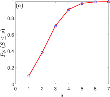
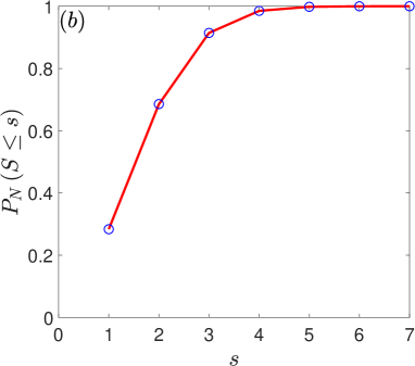
Figure 2: Exact analytical results (solid lines) for the cumulative distribution of the number of cycles in a directed 2-RRG (a) and an undirected 2-RRG (b) of $N=10$ nodes, obtained from Eqs. (33) and (57), respectively. The analytical results are in very good agreement with the results obtained from computer simulations (circles).

While Eq. (32) provides an exact result for $P_{N}(S=s)$, it is useful to express this distribution in terms of more elementary functions. This is possible in the asymptotic limit of large $N$. The limit of $N\gg 1$ corresponds to the limit of $z\rightarrow 1^{-}$ of the discrete Laplace transform $\widehat{f}_{s}(z)$ [27, 28]. If one replaces the variable $z$ by $e^{-x}$, then this limit corresponds to $x\ll 1$ in $\widehat{f}_{s}(e^{-x})$. In this limit the expression for $\widehat{f}_{s}\left(e^{-x}\right)$ in Eq. (25) can be approximated by

$$\widehat{f}_{s}\left(e^{-x}\right)\simeq\left(-\ln x\right)^{s}.$$ (34)

In order to calculate the inverse Laplace transform of $\widehat{f}_{s}\left(e^{-x}\right)$, we use the relation

$${\cal L}^{-1}\left[\frac{1}{x^{\nu}}(-\ln x)^{s}\right]=\left(\frac{d}{d\nu}\right)^{s}\left[\frac{N^{\nu-1}}{\Gamma(\nu)}\right],$$ (35)

where $\Gamma(\nu)$ is the Gamma function [25]. The inverse Laplace transform of Eq. (34) is obtained by taking the limit $\nu\rightarrow 0$ in Eq. (35). To this end we use the general Leibnitz rule (equation 1.4.12 in Ref. [25])

$$\left(\frac{d}{d\nu}\right)^{s}\left[\frac{N^{\nu-1}}{\Gamma(\nu)}\right]=\sum_{i=0}^{s}\binom{s}{i}\left[\left(\frac{d}{d\nu}\right)^{s-i}N^{\nu-1}\right]\left[\left(\frac{d}{d\nu}\right)^{i}\left(\frac{1}{\Gamma(\nu)}\right)\right].$$ (36)

Below we evaluate the derivatives that appear in the two terms on the right hand side of Eq. (36). The derivative in the first term is given by

$$\left(\frac{d}{d\nu}\right)^{i}N^{\nu-1}=N^{\nu-1}(\ln N)^{i}.$$ (37)

Thus, for $\nu\rightarrow 0^{+}$ we obtain

$$\lim_{\nu\rightarrow 0^{+}}\left[\left(\frac{d}{d\nu}\right)^{i}N^{\nu-1}\right]=\frac{(\ln N)^{i}}{N}.$$ (38)

The derivative in the second term on the right hand side of Eq. (36) is denoted by

$$h_{i}=\lim_{\nu\rightarrow 0^{+}}\left\{\left(\frac{d}{d\nu}\right)^{i}\left[\frac{1}{\Gamma(\nu)}\right]\right\}.$$ (39)

By its definition, $h_{i}$ is the coefficient of the $i$’th power of $\nu$ in the Taylor expansion of $1/\Gamma(\nu)$ around $\nu=0$, namely

$$\frac{1}{\Gamma(\nu)}=\sum_{i=1}^{\infty}\frac{h_{i}}{i!}\nu^{i}.$$ (40)

This expansion is often written as a power-series of the form [29, 30]

$$\frac{1}{\Gamma(\nu)}=\sum_{i=1}^{\infty}a_{i}\nu^{i},$$ (41)

where $a_{i}=h_{i}/i!$. The first two coefficients are given by $a_{1}=1$ and $a_{2}=\gamma$, where $\gamma$ is the Euler-Mascheroni constant [25]. Higher order coefficients can be obtained from the recursion equation

$$a_{i}=\frac{1}{i-1}\left[a_{2}a_{i-1}-\sum_{j=2}^{i-1}(-1)^{j}\zeta(j)a_{i-j}\right],$$ (42)

where $\zeta(j)$ is the Riemann zeta function. The coefficients $a_{i}$ for $i=3,4,\dots,10$, obtained from Eq. (42), are presented in Table I. These coefficients can also be obtained from the integral representation [31]

Table 1: The coefficients $a_{i}$, $i=1,2,\dots,10$, which appear in the power series of the reciprocal gamma function given by Eq. (42)

$i$	$a_{i}$
1	1
2	0.5772156649
3	- 0.6558780715
4	- 0.0420026350
5	0.1665386114
6	- 0.0421977345
7	- 0.0096219715
8	0.0072189432
9	- 0.0011651675
10	- 0.0002152416

$$a_{n}=\frac{(-1)^{n}}{\pi n!}\int_{0}^{\pi}e^{-t}{\rm Im}\left[(\ln t-i\pi)^{n}\right]dt.$$ (43)

Using this notation we obtain

$$f_{s}(N)\simeq\frac{s!}{N}\sum_{i=1}^{s}a_{i}\frac{(\ln N)^{s-i}}{(s-i)!},$$ (44)

which leads to

$$P_{N}(S=s)\simeq\frac{1}{N}\sum_{i=1}^{s}a_{i}\frac{(\ln N)^{s-i}}{(s-i)!}.$$ (45)

Note that for sufficiently large $N$ the sum is dominated by the first few terms for two reasons. First, apart from the first few terms, the coefficients $a_{i}$ become negligibly small. Second, the power of $\ln N$ decreases as $i$ is increased.

The cumulative distribution of the number of cycles is given by

$$P_{N}(S\leq s)=\frac{1}{N}\sum_{s^{\prime}=1}^{s}\sum_{i=1}^{s^{\prime}}a_{i}\frac{(\ln N)^{s^{\prime}-i}}{(s^{\prime}-i)!}.$$ (46)

In Fig. 3(a) we present analytical results (solid line) for the large $N$ approximation of the cumulative distribution $P_{N}(S\leq s)$ of the number of cycles in a directed 2-RRG of $N=10^{4}$ nodes, obtained from Eq. (46). The analytical results are found to be in very good agreement with the results obtained from computer simulations (circles).

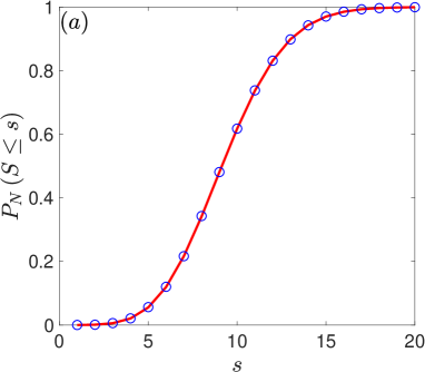
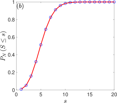
Figure 3: Analytical results (solid lines) for the cumulative distribution of the number of cycles in a directed 2-RRG (a) and an undirected 2-RRG (b) of $N=10^{4}$ nodes, obtained from Eqs. (46) and (60), respectively. The analytical results are in very good agreement with the results obtained from computer simulations (circles).

IV.2 Distribution of the number of cycles in undirected 2-RRGs

We now turn to calculate the distribution $P_{N}(S=s)$ of the number of cycles in undirected 2-RRGs. Inserting the expression for $P_{N}(\{g_{\ell}\})$ from Eq. (14) in Eq. (15), we obtain

$$P_{N}(S=s)=\frac{(2N)!!}{(2N-1)!!}\sum_{g_{1},\dots,g_{N}\geq 0}\prod_{\ell=1}^{N}\frac{1}{(2\ell)^{g_{\ell}}g_{\ell}!}\delta_{\sum_{\ell}\ell g_{\ell},N}\delta_{\sum_{\ell}g_{\ell},s}.$$ (47)

Using the change of variables presented in Eq. (18), we obtain

$$P_{N}(S=s)=\frac{(2N)!!}{(2N-1)!!}\frac{1}{2^{s}s!}\sum_{\ell_{1},\dots,\ell_{s}=1}^{N}\frac{1}{\ell_{1}\ell_{2}\dots\ell_{s}}\delta_{\sum_{i}\ell_{i},N}.$$ (48)

Note that the sum on the right hand side of Eq. (48) is equal to $f_{s}(N)$, given by Eq. (20). We thus obtain

$$P_{N}(S=s)=\frac{(2N)!!}{(2N-1)!!}\frac{1}{2^{s}N!}\bigg{[}\begin{array}[]{l}N\\ s\end{array}\bigg{]}.$$ (49)

Below we show that the distribution $P_{N}(S=s)$ is properly normalized. To this end we use equation 26.8.7 from Ref. [25], which can be written in the form

$$\sum_{s=1}^{N}(-1)^{N-s}\bigg{[}\begin{array}[]{l}N\\ s\end{array}\bigg{]}x^{s}=(x-N+1)_{N},$$ (50)

where $(a)_{N}$ is the Pochhammer symbol [25]. Inserting $x=-1/2$ in Eq. (50), we obtain

$$\sum_{s=1}^{N}\bigg{[}\begin{array}[]{l}N\\ s\end{array}\bigg{]}\frac{1}{2^{s}}=(-1)^{N}\left(\frac{1}{2}-N\right)_{N}.$$ (51)

Expressing the Pochhammer symbol on the right hand side of Eq. (51) as a ratio between two Gamma functions, we obtain

$$\sum_{s=1}^{N}\bigg{[}\begin{array}[]{l}N\\ s\end{array}\bigg{]}\frac{1}{2^{s}}=\frac{(-1)^{N}\Gamma(1/2)}{\Gamma(1/2-N)}.$$ (52)

Using Euler’s reflection formula [25]

$$\Gamma\left(\frac{1}{2}-N\right)\Gamma\left(\frac{1}{2}+N\right)=(-1)^{N}\pi,$$ (53)

and the Legendre duplication formula [25]

$$\Gamma(1/2+N)=2^{1-2N}\sqrt{\pi}\frac{\Gamma(2N)}{\Gamma(N)},$$ (54)

we obtain

$$\sum_{s=1}^{N}\bigg{[}\begin{array}[]{l}N\\ s\end{array}\bigg{]}\frac{1}{2^{s}}=2^{1-2N}\frac{\Gamma(2N)}{\Gamma(N)}.$$ (55)

Expressing the Gamma functions of integer variables in terms of factorials and double factorials, we obtain

$$\sum_{s=1}^{N}\bigg{[}\begin{array}[]{l}N\\ s\end{array}\bigg{]}\frac{1}{2^{s}}=\frac{(2N-1)!!}{(2N)!!}N!.$$ (56)

This confirms the normalization of $P_{N}(S=s)$, given by Eq. (49). From Eq. (49) we obtain the cumulative distribution of the number of cycles, which is given by

$$P_{N}(S\leq s)=\frac{(2N)!!}{(2N-1)!!}\frac{1}{N!}\sum_{s^{\prime}=1}^{s}\frac{1}{2^{s^{\prime}}}\bigg{[}\begin{array}[]{l}N\\ s^{\prime}\end{array}\bigg{]}.$$ (57)

In Fig. 2(b) we present exact analytical results (solid line) for the cumulative distribution $P(S\leq s)$ of the number of cycles in undirected 2-RRGs that consist of $N=10$ nodes, obtained from Eq. (57). The analytical results are found to be in very good agreement with the results obtained from computer simulations (circles).

While Eq. (49) provides an exact result for $P_{N}(S=s)$, it is useful to express this distribution in terms of more elementary functions. This is possible in the asymptotic limit of large $N$, where the ratio of double factorials can be approximated by

$$\frac{(2N)!!}{(2N-1)!!}\simeq\sqrt{\pi N}+O\left(N^{-1/2}\right).$$ (58)

Using this result and inserting $f_{s}(N)$ from Eq. (44) into Eq. (48), we find that

$$P_{N}(S=s)\simeq\frac{1}{2^{s}}\sqrt{\frac{\pi}{N}}\sum_{i=1}^{s}a_{i}\frac{(\ln N)^{s-i}}{(s-i)!}.$$ (59)

From Eq. (59) we obtain the cumulative distribution of the number of cycles, which is given by

$$P_{N}(S\leq s)\simeq\sqrt{\frac{\pi}{N}}\sum_{s^{\prime}=1}^{s}\frac{1}{2^{s^{\prime}}}\sum_{i=1}^{s^{\prime}}a_{i}\frac{(\ln N)^{s^{\prime}-i}}{(s^{\prime}-i)!}.$$ (60)

In Fig. 3(b) we present analytical results (solid line) for the cumulative distribution of the number of cycles in undirected 2-RRGs of $N=10^{4}$ nodes, obtained from Eq. (60). The analytical results are found to be in very good agreement with the results obtained from computer simulations (circles).

V Moments and cumulants

In this section we calculate the moments and cumulants of the distribution of the number of cycles in 2-RRGs that consist of $N$ nodes. To this end we introduce the moment generating function, which is given by

$$M(t)={\mathbb{E}}\left[e^{tS}\right].$$ (61)

The cumulant generating function is given by

$$K(t)=\ln M(t).$$ (62)

Using this function one can calculate the cumulants via differentiation according to

$$\kappa_{n}=\frac{d^{n}K(t)}{dt^{n}}\bigg{|}_{t=0}.$$ (63)

V.1 Moments and cumulants in directed 2-RRGs

The moment generating function of directed 2-RRGs is given by

$$M(t)=\frac{1}{N!}\sum_{s=0}^{N}e^{ts}\bigg{[}\begin{array}[]{l}N\\ s\end{array}\bigg{]}.$$ (64)

Using Eq. (50) with $x=-e^{t}$, we obtain

$$M(t)=\frac{(-1)^{N}}{N!}\left(-e^{t}-N+1\right)_{N}.$$ (65)

The moment generating function $M(t)$ may also be written in the form

$$M(t)=\frac{\Gamma(N+e^{t})}{\Gamma(e^{t})N!},$$ (66)

in agreement with the results presented in Ref. [16]. The corresponding cumulant generating function is given by

$$K(t)=\ln\left[\frac{\Gamma(N+e^{t})}{\Gamma(e^{t})N!}\right].$$ (67)

Using Eq. (67) we obtain the first two cumulants, which are given by

$$\langle S\rangle=\kappa_{1}=H_{N},$$ (68)

where $H_{N}$ is the harmonic number [32], and

$${\rm Var}(S)=\kappa_{2}=H_{N}-H_{N}^{(2)},$$ (69)

where $H_{N}^{(m)}$ is the generalized harmonic number of order $m$ [32]. Similarly, one can calculate higher order cumulants such as

$$\kappa_{3}=H_{N}-3H_{N}^{(2)}+2H_{N}^{(3)}$$ (70)

and

$$\kappa_{4}=H_{N}-7H_{N}^{(2)}+12H_{N}^{(3)}-6H_{N}^{(4)}.$$ (71)

In the limit of large $N$ we can use the asymptotic expression for the distribution $P_{N}(S=s)$, given by Eq. (45), and obtain

$$M(t)\simeq\frac{1}{N}\sum_{s=0}^{\infty}\sum_{i=1}^{s}e^{st}a_{i}\frac{(\ln N)^{s-i}}{(s-i)!}.$$ (72)

Exchanging the order of summations, we obtain

$$M(t)\simeq\frac{1}{N}\sum_{i=1}^{\infty}a_{i}\sum_{s=i}^{\infty}e^{st}\frac{(\ln N)^{s-i}}{(s-i)!}.$$ (73)

Shifting the summation index in the second sum, we obtain

$$M(t)\simeq\frac{1}{N}\sum_{i=1}^{\infty}a_{i}e^{it}\sum_{s=0}^{\infty}e^{st}\frac{(\ln N)^{s}}{s!}.$$ (74)

Using Eq. (41) we carry out the two summations and obtain

$$M(t)\simeq\frac{1}{N}\frac{1}{\Gamma(e^{t})}\exp\left(e^{t}\ln N\right).$$ (75)

Using Eq. (62) we obtain the cumulant generating function, which is given by

$$K(t)\simeq\left(e^{t}-1\right)\ln N-\ln\left[\Gamma\left(e^{t}\right)\right].$$ (76)

Using Eq. (63) we obtain the cumulants, which take the form

$$\kappa_{n}\simeq\ln N-\frac{d^{n}}{dt^{n}}\ln\left[\Gamma\left(e^{t}\right)\right]\bigg{|}_{t=0}.$$ (77)

In order to calculate high order derivatives of $\ln\left[\Gamma\left(e^{t}\right)\right]$ we use the identity (equation A.4 in Ref. [32])

$$\frac{d^{n}}{dt^{n}}f(e^{t})=\sum_{m=1}^{n}\bigg{\{}\begin{array}[]{l}n\\ m\end{array}\bigg{\}}e^{mt}f^{(m)}(e^{t}),$$ (78)

where $\bigg{\{}\begin{array}[]{l}n\\ m\end{array}\bigg{\}}$ is the Stirling number of the second kind and $f^{(m)}(x)$ is the $m$th derivative of $f(x)$. We also use the fact that

$$\frac{d^{n}}{dz^{n}}\ln\Gamma(z)=\psi^{(n-1)}(z),$$ (79)

where $\psi^{(n)}(z)$ is the $n$th derivative of the digamma function [25]. Using these identities, we obtain

$$\frac{d^{n}}{dt^{n}}\ln\left[\Gamma\left(e^{t}\right)\right]\bigg{|}_{t=0}=\sum_{m=1}^{n}\bigg{\{}\begin{array}[]{l}n\\ m\end{array}\bigg{\}}\psi^{(m-1)}(1).$$ (80)

It is also known that (equation 5.4.12 in Ref. [25])

$$\psi^{(0)}(1)=-\gamma,$$ (81)

and that for $m\geq 1$ (equation 5.15.2 in Ref. [25])

$$\psi^{(m)}(1)=(-1)^{m+1}m!\zeta(m+1),$$ (82)

where $\zeta(m)$ is the Riemann zeta function [25]. Combining the results derived above, we obtain

$$\kappa_{n}\simeq\ln N+\gamma+\sum_{m=2}^{n}\bigg{\{}\begin{array}[]{l}n\\ m\end{array}\bigg{\}}(-1)^{m-1}(m-1)!\zeta(m).$$ (83)

Using Eq. (83) we write down explicitly the first few cumulants of $P_{N}(S=s)$ in the large $N$ limit. They are given by

$$\kappa_{1} \simeq \ln N+\gamma$$

$$\kappa_{2} \simeq \ln N+\gamma-\frac{\pi^{2}}{6}$$

$$\kappa_{3} \simeq \ln N+\gamma-\frac{\pi^{2}}{2}+2\zeta(3)$$

$$\kappa_{4} \simeq \ln N+\gamma-\frac{7\pi^{2}}{6}+12\zeta(3)-\frac{\pi^{4}}{15}.$$ (84)

The results for $\kappa_{1}$ and $\kappa_{2}$ are in agreement with the classical results reported in Refs. [33, 34, 35, 36]. In the large $N$ limit all the cumulants are of the form $\ln N+{\cal O}(1)$. This essentially implies that in the large $N$ limit the distribution $P_{N}(S=s)$ approaches a Poisson distribution with a parameter $\ln N$.

Comparing between Eqs. (68)-(71) and Eq. (83), and using the fact that for $m\geq 2$

$$\lim_{N\rightarrow\infty}H_{N}^{(m)}=\zeta(m),$$ (85)

we obtain a general expression for the cumulants at finite values of $N$, which is given by

$$\kappa_{n}=H_{N}+\sum_{m=2}^{n}\bigg{\{}\begin{array}[]{l}n\\ m\end{array}\bigg{\}}(-1)^{m-1}(m-1)!H_{N}^{(m)}.$$ (86)

In Fig. 4 we present analytical results (solid line) for the mean number of cycles $\langle S\rangle$ in directed 2-RRGs as a function of the network size $N$, obtained from Eq. (68). The analytical results are in very good agreement with the results obtained from computer simulations (circles).

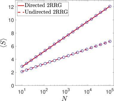
Figure 4: Analytical results for the mean number of cycles $\langle S\rangle$ as a function of the network size $N$, in directed 2-RRGs (solid line) and in undirected 2-RRGs (dashed line), obtained from Eqs. (68) and (91), respectively. The analytical results are in very good agreement with the results obtained from computer simulations (circles). To leading order, in directed 2-RRGs $\langle S\rangle\simeq\ln N$, while in undirected 2-RRGs $\langle S\rangle\simeq\frac{1}{2}\ln N$.

In Fig. 5 we present analytical results (solid line) for the variance ${\rm Var}(S)$ in directed 2-RRGs as a function of the network size $N$, obtained from Eq. (69). The analytical results are in very good agreement with the results obtained from computer simulations (circles).

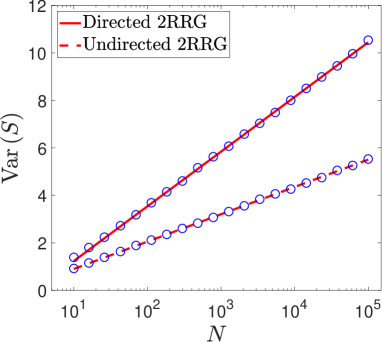
Figure 5: Analytical results for the variance of the distribution of the number of cycles as a function of the network size $N$, in directed 2-RRGs (solid line) and in undirected 2-RRGs (dashed line), obtained from Eqs. (69) and (92), respectively. The analytical results are in very good agreement with the results obtained from computer simulations (circles). To leading order, in directed 2-RRGs ${\rm Var}(S)\simeq\ln N$, while in undirected 2-RRGs ${\rm Var}(S)\simeq\frac{1}{2}\ln N$.

V.2 Moments and cumulants in undirected 2-RRGs

The moment generating function of undirected 2-RRGs is given by

$$M(t)=\frac{(2N)!!}{(2N-1)!!}\frac{1}{N!}\sum_{s=0}^{N}\frac{e^{ts}}{2^{s}}\bigg{[}\begin{array}[]{l}N\\ s\end{array}\bigg{]}.$$ (87)

Using Eq. (50) with $x=-e^{t}/2$, we obtain

$$M(t)=\frac{(-1)^{N}}{N!}\frac{(2N)!!}{(2N-1)!!}\left(-\frac{e^{t}}{2}-N+1\right)_{N}.$$ (88)

The moment generating function $M(t)$ may also be written in the form

$$M(t)=\frac{(2N)!!}{(2N-1)!!}\frac{\Gamma\left(N+\frac{e^{t}}{2}\right)}{\Gamma\left(\frac{e^{t}}{2}\right)N!}.$$ (89)

The corresponding cumulant generating function is given by

$$K(t)=\ln\left[\frac{(2N)!!}{(2N-1)!!}\frac{\Gamma\left(N+\frac{e^{t}}{2}\right)}{\Gamma\left(\frac{e^{t}}{2}\right)N!}\right].$$ (90)

Using Eq. (63) we obtain the first four cumulants. The first cumulant is given by

$$\langle S\rangle=\kappa_{1}=\frac{1}{2}H_{N-\frac{1}{2}}+\ln 2,$$ (91)

where $H_{N-\frac{1}{2}}$ is an Harmonic number at a half-integer value [37]. The second cumulant is given by

$${\rm Var}(S)=\kappa_{2}=\frac{1}{2}H_{N-\frac{1}{2}}+\ln 2-\frac{1}{4}\left[H_{N-\frac{1}{2}}^{(2)}+2\zeta(2)\right],$$ (92)

while the third and fourth cumulants are given by

$$\kappa_{3}=\frac{1}{2}H_{N-\frac{1}{2}}+\ln 2-\frac{3}{4}\left[H_{N-\frac{1}{2}}^{(2)}+2\zeta(2)\right]+\frac{1}{4}\left[H_{N-\frac{1}{2}}^{(3)}+6\zeta(3)\right]$$ (93)

and

$$\kappa_{4}=\frac{1}{2}H_{N-\frac{1}{2}}+\ln 2-\frac{7}{4}\left[H_{N-\frac{1}{2}}^{(2)}+2\zeta(2)\right]+\frac{3}{2}\left[H_{N-\frac{1}{2}}^{(3)}+6\zeta(3)\right]-\frac{3}{8}\left[H_{N-\frac{1}{2}}^{(4)}+14\zeta(4)\right].$$ (94)

In the limit of large $N$ we can use the asymptotic expression for the distribution $P_{N}(S=s)$, given by Eq. (59). Inserting it into Eq. (61) we obtain an asymptotic expression for the moment generating function, which is given by

$$M(t)\simeq\sqrt{\frac{\pi}{N}}\sum_{s=0}^{\infty}\sum_{i=1}^{s}e^{st}\frac{a_{i}}{2^{i}}\frac{(\ln N)^{s-i}}{2^{s-i}(s-i)!}.$$ (95)

Exchanging the order of summations and shifting the summation index in the second sum, we obtain

$$M(t)\simeq\sqrt{\frac{\pi}{N}}\sum_{i=1}^{\infty}a_{i}\frac{e^{it}}{2^{i}}\sum_{s=0}^{\infty}e^{st}\frac{(\ln N)^{s}}{2^{s}s!}.$$ (96)

Using Eq. (41) we carry out the two summations and obtain

$$M(t)\simeq\sqrt{\frac{\pi}{N}}\frac{1}{\Gamma(e^{t}/2)}\exp\left(\frac{e^{t}}{2}\ln N\right).$$ (97)

Using Eq. (62) we obtain the cumulant generating function, which is given by

$$K(t)\simeq\frac{e^{t}-1}{2}\ln N-\ln\left[\frac{1}{\sqrt{\pi}}\Gamma\left(\frac{e^{t}}{2}\right)\right].$$ (98)

Using Eq. (63) we obtain the cumulants, which take the form

$$\kappa_{n}\simeq\frac{1}{2}\ln N-\frac{d^{n}}{dt^{n}}\ln\left[\frac{1}{\sqrt{\pi}}\Gamma\left(\frac{e^{t}}{2}\right)\right]\bigg{|}_{t=0}.$$ (99)

Using Eqs. (78) and (79), we obtain

$$\frac{d^{n}}{dt^{n}}\ln\left[\frac{1}{\sqrt{\pi}}\Gamma\left(\frac{e^{t}}{2}\right)\right]\bigg{|}_{t=0}=\sum_{m=1}^{n}\bigg{\{}\begin{array}[]{l}n\\ m\end{array}\bigg{\}}2^{-m}\psi^{(m-1)}\left(\frac{1}{2}\right).$$ (100)

It is also known that [38]

$$\psi^{(0)}\left(\frac{1}{2}\right)=-\gamma-\ln 4,$$ (101)

and that for $m\geq 1$ [38]

$$\psi^{(m)}\left(\frac{1}{2}\right)=(-1)^{m+1}m!\left(2^{m+1}-1\right)\zeta(m+1).$$ (102)

Combining the results derived above, we obtain

$$\kappa_{n}\simeq\frac{\ln N}{2}+\frac{\gamma+\ln 4}{2}+\sum_{m=2}^{n}\bigg{\{}\begin{array}[]{l}n\\ m\end{array}\bigg{\}}(-1)^{m-1}\left(1-2^{-m}\right)(m-1)!\zeta(m),$$ (103)

which becomes exact in the large $N$ limit. Using Eq. (103) we write down explicitly the first few cumulants of $P_{N}(S=s)$. They are given by

$$\kappa_{1} \simeq \frac{\ln N}{2}+\frac{\gamma+\ln 4}{2}$$

$$\kappa_{2} \simeq \frac{\ln N}{2}+\frac{\gamma+\ln 4}{2}-\frac{\pi^{2}}{8}$$

$$\kappa_{3} \simeq \frac{\ln N}{2}+\frac{\gamma+\ln 4}{2}-\frac{3\pi^{2}}{8}+\frac{7}{4}\zeta(3)$$

$$\kappa_{4} \simeq \frac{\ln N}{2}+\frac{\gamma+\ln 4}{2}-\frac{7\pi^{2}}{8}+\frac{21}{2}\zeta(3)-\frac{\pi^{4}}{16}.$$ (104)

In the large $N$ limit all the cumulants are of the form $\frac{1}{2}\ln N+{\cal O}(1)$. This essentially implies that in the large $N$ limit the distribution $P_{N}(S=s)$ approaches a Poisson distribution with a parameter $\frac{1}{2}\ln N$.

Using the fact that for $m\geq 2$

$$\lim_{N\rightarrow\infty}H_{N-\frac{1}{2}}^{(m)}=\zeta(m),$$ (105)

we obtain a general expression for the cumulants at finite values of $N$, which is given by

$$\kappa_{n}=\frac{1}{2}H_{N-\frac{1}{2}}+\ln 2+\sum_{m=2}^{n}\bigg{\{}\begin{array}[]{l}n\\ m\end{array}\bigg{\}}(-1)^{m-1}2^{-m}(m-1)!\left[H_{N-\frac{1}{2}}^{(m)}+(2^{m}-2)\zeta(m)\right].$$ (106)

In Fig. 4 we present analytical results (dashed line) for the mean number of cycles $\langle S\rangle$ in undirected 2-RRGs as a function of the network size $N$, obtained from Eq. (91). The analytical results are in very good agreement with the results obtained from computer simulations (circles).

In Fig. 5 we present analytical results (dashed line) for the variance ${\rm Var}(S)$ in undirected 2-RRGs as a function of the network size $N$, obtained from Eq. (92). The analytical results are in very good agreement with the results obtained from computer simulations (circles).

VI Discussion

Below we discuss the similarities and differences between the directed and undirected 2-RRGs. In directed 2-RRGs the mean number of cycles $\langle S\rangle$ scales with $\ln N$, while in undirected 2-RRGs it scales with $\frac{1}{2}\ln N$. Thus, the expected number of cycles in directed 2-RRGs is twice as large as in undirected 2-RRGs. This is due to the fact that in the construction of undirected 2-RRGs each end of a given chain may connect to both sides of any other linear chain, while in directed 2-RRGs it may only connect to the complementary side. As a result, in undirected 2-RRGs the connection of chains forming a longer chain is more probable than in directed 2-RRGs. Thus, in undirected 2-RRGs the competing process of closing a chain to form a cycle is less probable than in directed 2-RRGs. This implies that in undirected 2-RRGs the cycles are expected to be longer and their number is expected to be smaller than in directed 2-RRGs.

2-RRGs are marginal networks that reside at the boundary between the subcritical regime and the supercritical regime. In the subcritical regime, configuration model networks consist of many finite tree components. The distribution of sizes of these tree components can be calculated using the framework of generating functions [39]. In this framework it is assumed that all the network components exhibit a tree structure. In the 2-RRG the topological constraint that all the nodes are of degree $k=2$ imposes the formation of cycles. Therefore, the generating function formalism cannot be used to analyze the distribution of cycle lengths in 2-RRGs. A naive attempt to use the generating function formalism to obtain the distribution of cluster sizes (which are also the cycle lengths) in 2-RRGs fails to determine the distribution.

RRGs with $c\geq 3$ are supercritical. They consist of a giant component that encompasses the whole network. While the local structure of the the network is typically tree-like, at larger scales it exhibits cycles with a broad distribution of cycle lengths. The length of a cycle is given by the number of nodes (or edges) that reside along the cycle. The longest possible cycle is a Hamiltonian cycle of length $\ell=N$. The expected number of cycles of length $\ell$ in an undirected RRG that consists of $N$ nodes of degree $c\geq 3$, where $\ell\ll\ln N$, is given by [40, 41, 42]

$$\langle G_{\ell}\rangle=\frac{(c-1)^{\ell}}{2\ell}.$$ (107)

This implies that for $c\geq 3$ the number of cycles of length $\ell$ proliferates exponentially as $\ell$ is increased, as long as $\ell\ll\ln N$. Although these results were not claimed to hold in the case of $c=2$, it is interesting to examine their relevance to 2-RRGs. In the special case of an undirected 2-RRG, where $c=2$, Eq. (107) is reduced to

$$\langle G_{\ell}\rangle=\frac{1}{2\ell}.$$ (108)

In Fig. 6 we present analytical results (solid lines) for the expected number $\langle G_{\ell}\rangle$ of cycles of length $\ell$ in undirected 2-RRGs, obtained from Eq. (108), as a function of $\ell$ for $N=10$ (a) and $N=10^{4}$ (b). We also present the results obtained from computer simulations (circles). It is found that for $N=10$ there is a big difference between the analytical results obtained from Eq. (108) and the simulation results. In contrast, for $N=10^{4}$ the analytical results are in very good agreement with the results of computer simulations for $\ell\ll N$. This implies that Eq. (108) is valid for 2-RRGs in the large network limit and for sufficiently short cycles. For larger values of $\ell$ Eq. (108) is no longer valid, as $\langle G_{\ell}\rangle$ becomes an increasing function of $\ell$. Note that the simulation results for $\langle G_{\ell}\rangle$ exceed the values predicted by Eq. (108). The total number of nodes can be expressed in the form

$$N=\sum_{\ell=1}^{N}\ell\langle G_{\ell}\rangle,$$ (109)

which is obtained by averaging Eq. (6) over the ensemble. Inserting $\langle G_{\ell}\rangle$ from Eq. (108) into the right hand side of Eq. (109), it yields only $N/2$ nodes instead of $N$ nodes. This implies that Eq. (108) is valid only as long as $\ell\ll N$. Indeed, Fig. 6 reveals that Eq. (108) misses the very long cycles whose length is of order $N$.

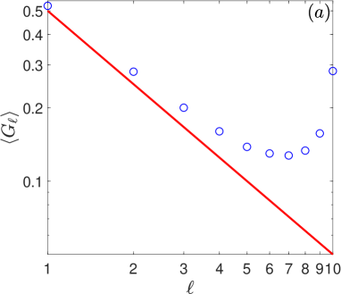
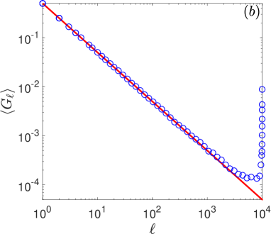
Figure 6: Analytical results (solid lines) for the expected number $\langle G_{\ell}\rangle$ of cycles of length $\ell$, in an undirected 2-RRG that consists of $N$ nodes, for $N=10$ (a) and for $N=10^{4}$ (b), obtained from Eq. (108), on a log-log scale. We also present results obtained from computer simulations (circles). For $N=10$ the simulation results deviate significantly from the prediction of Eq. (108). For $N=10^{4}$ there is a very good agreement between the analytical results and the simulation results in the range of $\ell\ll N$. The agreement between the analytical results and the simulation results improves as $N$ is increased.

VII Summary

2-RRGs are networks in which each node has two links. Therefore, these networks consist of a set of closed cycles whose lengths are determined by the random process of bond formation between the nodes. In this paper we have calculated the distributions $P_{N}(S=s)$ of the number of cycles in directed and undirected 2-RRGs. Starting from the joint distributions of cycle lengths $P_{N}(\{g_{\ell}\})$ we obtained exact results for $P_{N}(S=s)$, which are expressed in terms of the Stirling numbers of the first kind. In sufficiently large networks these distributions can be expressed in terms of more elementary functions. We also derived closed-form expressions for the moments and cumulants of $P_{N}(S=s)$. It was found that to leading order, in directed 2-RRGs, the cumulants of all orders $n=1,2,\dots$ satisfy $\kappa_{n}\simeq\ln N$, while in undirected 2-RRGs they satisfy $\kappa_{n}\simeq\frac{1}{2}\ln N$. This implies that in the large $N$ limit the distributions $P_{N}(S=s)$ converge towards the Poisson distribution.

This work was supported by the Israel Science Foundation grant no. 1682/18.

References

- [1] B. Bollobás, Random Graphs, Second Edition (Cambridge University Press, Cambridge, 2001).
- [2] S.N. Dorogovtsev and J.F.F. Mendes, Evolution of Networks: From Biological Nets to the Internet and WWW (Oxford University Press, Oxford, 2003).
- [3] S. Havlin and R. Cohen, Complex Networks: Structure, Robustness and Function (Cambridge University Press, New York, 2010).
- [4] E. Estrada, The structure of complex networks: Theory and applications (Oxford University Press, Oxford, 2011).
- [5] A. Barrat, M. Barthélemy and A. Vespignani, Dynamical Processes on Complex Networks (Cambridge University Press, Cambridge, 2012).
- [6] V. Latora, V. Nicosia and G. Russo, Complex Networks: Principles, Methods and Applications (Cambridge University Press, Cambridge, 2017).
- [7] M.E.J. Newman, Networks: an Introduction, Second Edition (Oxford University Press, Oxford, 2018).
- [8] R. van der Hofstad, Random graphs and complex networks (Cambridge University Press, Cambridge, 2016).
- [9] S.N. Dorogovtsev and J.F.F. Mendes, The Nature of Complex Networks (Oxford University Press, Oxford, 2022).
- [10] B. Bollobás, A probabilistic proof of an asymptotic formula for the number of labelled regular graphs, Euro. J. Combin. 1, 311 (1980).
- [11] M. Molloy and A. Reed, A critical point for random graphs with a given degree sequence, Random Structures and Algorithms 6, 161 (1995).
- [12] M. Molloy and A. Reed, The size of the giant component of a random graph with a given degree sequence, Combin., Prob. and Comp. 7, 295 (1998).
- [13] M.E.J. Newman, S.H. Strogatz and D.J. Watts, Random graphs with arbitrary degree distributions and their applications, Phys. Rev. E 64, 026118 (2001).
- [14] B.K. Fosdick, D.B. Larremore, J. Nishimura and J. Ugander, Configuring random graph models with fixed degree sequences, SIAM Review 60, 315 (2018).
- [15] R. Arratia and S. Tavaré, The cycle structure of random permutations, The Annals of Probability 20, 1567 (1992).
- [16] L.A. Shepp and S.P. Lloyd, Ordered cycle lengths in a random permutation, Transactions of the American Mathematical Society 121, 340 (1966).
- [17] P. Flajolet and A.M. Odlyzko, Random mapping statistics, Advances in Cryptography, J.J. Quisquater and J. Vandewalle (Eds.) Eurocrypt ’89, LNCS 434, 329 (1990)
- [18] S. W. Golomb, Random permutations, Bull. Amer. Math. Soc. 70, 747 (1964).
- [19] S. W. Golomb, Shift Register Sequences, Third Edition (World Scientific, Singapore, 2017).
- [20] M. Bóna, Combinatorics of Permutations, Second Edition (CRC Press, Boca Raton, 2012).
- [21] K. Dickman, On the frequency of numbers containing prime factors of a certain relative magnitude, Ark. Mat. Astron. Fysik 22A, 1 (1930).
- [22] S. R. Finch, Mathematical Constants, (Cambridge University Press, Cambridge, 2003).
- [23] S. W. Golomb and P. Gaal, On the number of permutations on objects with greatest cycle length , Adv. Appl. Math. 20, 98 (1998).
- [24] D. E. Knuth and L. Trabb Pardo, Analysis of a simple factorization algorithm, Theoret. Comput. Sci. 3, 321 (1976).
- [25] F.W.J. Olver, D.M. Lozier, R.F. Boisvert and C.W. Clark, NIST handbook of mathematical functions (Cambridge University Press, Cambridge, 2010).
- [26] C.L. Phillips, H.T. Nagle and A. Chakrabortty, Digital Control System: Analysis and Design, Fourth Edition (Pearson Education, Harlow, 2015).
- [27] O. Schlömilch, Recherches sur les coefficients des facultés analytiques, Crelle 44, 344 (1852).
- [28] E.C. Titchmarsh, The Theory of Functions, Second Edition (Oxford University Press, Oxford, 1939).
- [29] J.W. Wrench, Concerning two series for the gamma function, Mathematics of Computation 22, 617 (1968).
- [30] J.W. Wrench, Erratum: Concerning two series for the gamma function, Mathematics of Computation 27, 681 (1973).
- [31] L. Fekih-Ahmed, On the Power Series Expansion of the Reciprocal Gamma Function, HAL archives, https://hal.archives-ouvertes.fr/hal-01029331v1, arXiv:1407.5983.
- [32] K.N. Boyadzhiev, Notes on the Binomial Transform (World Scientific, Singapore, 2018).
- [33] W. Goncharov, Sur la distribution des cycles dans les permutations, C. R. (Dokl.) Acad. Sci. URSS 35, 267 (1942).
- [34] W. Goncharov, On the field of combinatory analysis, Soviet Math. Izv., Ser. Math 8, 3 (1944).
- [35] R. E. Greenwood, The number of cycles associated with the elements of a permutation group, Amer. Math. Monthly 60, 407 (1953).
- [36] H. S. Wilf, generatingfunctionology, Third Edition (A K Peters, Wellesley, 2005).
- [37] A. Sofo, Hamonic numbers at half-integer values, Integral Transforms and Special Functions 27, 430 (2016).
- [38] J. Choi and D. Cvijović, Values of the polygamma functions at rational arguments, J. Phys. A 40, 15019 (2007).
- [39] M.E.J. Newman, Component sizes in networks with arbitrary degree distributions, Phys. Rev. E 76, 045101 (2007).
- [40] E. Marinari and R. Monasson, Circuits in random graphs: from local trees to global loops, J. Stat. Mech., P09004 (2004).
- [41] G. Bianconi and M. Marsili, Loops of any size and Hamilton cycles in random scale-free networks J. Stat. Mech., P06005 (2005).
- [42] E. Marinari and G. Semerjian, On the number of circuits in random graphs, J. Stat. Mech., P06019 (2006).