Implementations of two Algorithms for the
Threshold Synthesis Problem

Abstract

A linear pseudo-Boolean constraint (LPB) is an expression of the form

$$a_{1}\cdot\ell_{1}+\ldots+a_{m}\cdot\ell_{m}\geq d,$$

where each $\ell_{i}$ is a literal (it assumes the value 1 or 0 depending on whether a propositional variable $x_{i}$ is true or false) and $a_{1},\ldots,a_{m},d$ are natural numbers. An LPB represents a Boolean function, and those Boolean functions that can be represented by exactly one LPB are called threshold functions. The problem of finding an LPB representation of a Boolean function if possible is called threshold recognition problem or threshold synthesis problem. The problem has an $O(m^{7}t^{5})$ algorithm using linear programming, where $m$ is the dimension and $t$ the number of terms in the DNF input. It has been an open question whether one can recognise threshold functions through an entirely combinatorial procedure. Smaus has developed such a procedure for doing this, which works by decomposing the DNF and “counting” the variable occurrences in it. We have implemented both algorithms as a thesis project. We report here on this experience. The most important insight was that the algorithm by Smaus is, unfortunately, incomplete.

1 Introduction

A linear pseudo-Boolean constraint (LPB) (?; ?) is an expression of the form $a_{1}\ell_{1}+\ldots+a_{m}\ell_{m}\geq d$. Here each $\ell_{i}$ is a literal of the form $x_{i}$ or $\bar{x}_{i}\equiv 1-x_{i}$, i.e. $x_{i}$ becomes 0 if $x_{i}$ is false and 1 if $x_{i}$ is true, and vice versa for $\bar{x}_{i}$. Moreover, $a_{1},\ldots,a_{m},d$ are natural numbers.

An LPB can be used to represent a Boolean function; e.g. $x_{1}+\bar{x}_{2}+x_{3}\geq 3$ represents the same function as the propositional formula $x_{1}\land\lnot x_{2}\land x_{3}$. It has been observed that a function can be often represented more compactly as a set of LPBs than as a conjunctive or disjunctive normal form (CNF or DNF) (?; ?). E.g. the LPB $2x_{1}+\bar{x}_{2}+x_{3}+x_{4}\geq 2$ corresponds to the DNF $x_{1}\lor(\lnot x_{2}\land x_{3})\lor(\lnot x_{2}\land x_{4})\lor(x_{3}\land x_{4})$, which has four clauses.

In this work we are concerned with functions that can be represented by a single LPB, the so-called threshold functions. The problem of recognising a Boolean function given in DNF as threshold function and computing the LPB representation if possible, is called threshold recognition problem or threshold synthesis problem. The problem is known to have an $O(m^{7}t^{5})$ algorithm using linear programming, where $m$ is the dimension and $t$ the number of terms in the DNF (?).

It has been an open question for decades whether it is possible to recognise threshold functions through an entirely combinatorial procedure, i.e., without resorting to the equivalent linear program. Smaus has developed a procedure, which works by decomposing the DNF and “counting” its variable occurrences in an appropriate way (?).

Schilling and Wenzelmann, students of Freiburg University, have implemented the classical linear programming algorithm and the more recent combinatorial algorithm, respectively, as Bachelor thesis projects (?; ?). We report here on this experience. The most important insight was that the algorithm by Smaus is, unfortunately, incomplete.

This paper is organised as follows. We continue with some preliminaries. Sec. 3 describes the linear programming algorithm, Sec. 4 the combinatorial procedure, Sec. 5 the implementation, and Sec. 6 concludes and discusses future work.

2 Preliminaries

We assume the reader to be familiar with the basic notions of propositional logic.

An $m$-dimensional Boolean function $f$ is a function $\mathit{Bool}^{m}\to\mathit{Bool}$. A linear pseudo-Boolean constraint (LPB) is an inequality of the form

$$a_{1}\ell_{1}+\ldots+a_{m}\ell_{m}\geq d\qquad a_{i}\in\mathbb{N},d\in\mathbb{Z},\ell_{i}\in\{x_{i},\bar{x}_{i}\}.$$ (1)

We call the $a_{i}$ coefficients and $d$ the degree (?). An occurrence of a literal $x_{i}$ (resp., $\bar{x}_{i}$) is called an occurrence of $x_{i}$ in positive (resp., negative) polarity. Note that if $d\leq 0$, then the LPB is a tautology. The reason for allowing for negative $d$ will become apparent in Subsec. 4.2.

A DNF is a formula of the form $c_{1}\lor\ldots\lor c_{n}$ where each clause $c_{j}$ is a conjunction of literals. Formally, a DNF is a set of sets of literals, i.e., the order of clauses and the order of literals within a clause are insignificant. For DNFs, we assume without loss of generality that no clause is a subset of another clause (the latter clause would be redundant since it is absorbed). We call a DNF prime irredundant if every clause is a prime implicant, i.e., if for clause $c_{1}$ there is no clause $c_{2}\neq c_{1}$ such that $c_{1}\lor c_{2}=c_{2}$. Any Boolean function can be represented by a DNF (?).

It is easy to see that an LPB can only represent monotone functions, i.e., functions represented by a DNF where each variable occurs in only one polarity. Hence any DNF containing a variable in different polarities is immediately uninteresting for us. Without loss of generality, we assume that this polarity is positive.

3 The linear programming algorithm

We shortly summarise the solution via linear programming, established by Peled & Simeone (?; ?).

For some DNFs, it is possible to establish a complete order $\succeq$ on the variables which, intuitively speaking, has the following meaning: $x_{i}\succeq x_{j}$ iff starting from any given input tuple $X^{*}\in\mathit{Bool}^{m}$, setting $x_{i}^{*}$ to true is more likely to make the DNF true than setting $x_{j}^{*}$ true. The functions represented by such a DNF are called regular.

The algorithm first tests the input DNF for the regularity property. The property is weaker than the threshold property, and so if a DNF is not regular, then it is not convertible and we must give up.

The order is established by counting the variables in a special way. Intuitively, a variable is “important” if it occurs in many clauses and if it occurs in short clauses. This is formalised as the so-called occurrence pattern of a variable $x$ in $\phi$, written $\mathit{OP}(\phi,x)$. For space reasons, we do not give the formal definition and refer the reader to (?).

Computing the set of occurrence patterns for all variables in $\phi$ can be done in time linear in the size of $\phi$ as it can be done in a single pass over $\phi$. In fact, the number of elements of all occurrence patterns is exactly the number of literals in $\phi$. Thus sorting the variables w.r.t. the occurrence patterns can be done in time polynomial in $|\phi|$.

The notion of occurrence patterns is equivalent to the so-called Winder matrix (?). We will need the concept again in the next section.

Provided the DNF is regular, we make use of the minimal true points of the DNF, i.e. the true tuples where we cannot set any 1-value to 0 without making the point false. We also use the maximal false points defined analogously. Note that these together characterise the DNF uniquely. In general, no polynomial algorithm is known to find these points (which is no surprise since the general task is NP-complete (?)), but for the special case that the input DNF is prime irredundant this is possible. The reason is that the true points can be read directly from the clauses. It is for this reason that we require the input DNF to be in prime irredundant form.

Having these, there exists a polynomial time procedure to find the maximal false points. Then we can formulate the following linear program where the minimal true points are $x^{1},\dots,x^{k}$ and the maximal false points are $y^{1},\dots,y^{l}$:

$$\sum_{i=1}^{m}a_{i}x_{i}^{j} \geq d (1\leq j\leq k)$$

$$\sum_{i=1}^{m}a_{i}y_{i}^{j} < d (1\leq j\leq l)$$

$$a_{i} \geq 0 (1\leq i\leq m)$$

Note that the weights $a_{i}$ are the variables in the LP formulation and the threshold is $d$. Finally, the linear program is passed to an LP solver. The reason for the complexity blow-up ($O(m^{7}t^{5})$ where $m$ is the dimension and $t$ the number of terms in the DNF) is mainly due to the linear programming. The other parts run in $O(m^{2}t)$, so the whole procedure gains from future improvements of linear programming. It should be mentioned that for most inputs the well-known simplex method for solving linear programs runs in linear time.

4 The combinatorial algorithm

In this section we recall the results from our previous work (?) and present an algorithm for the problem of converting a DNF to an equivalent LPB if possible.

4.1 Determining the order of coefficients

Given a DNF $\phi$, if $\phi$ can be represented as an LPB at all, then the coefficients must respect the order $\succeq$ introduced in the previous section, i.e., $\mathit{OP}(\phi,x_{i})\succeq\mathit{OP}(\phi,x_{k})$ implies that $a_{i}\geq a_{k}$ in the resulting LPB:

Lemma 4.1

Let $\phi$ be a DNF represented by the LPB $\sum_{i=1}^{m}a_{i}x_{i}\geq d$. Then $a_{i}\geq a_{k}$ implies $\mathit{OP}(\phi,x_{i})\succeq\mathit{OP}(\phi,x_{k})$; moreover, there exists an LPB $\sum_{i=1}^{m}a^{\prime}_{i}x_{i}\geq d^{\prime}$ representing $\phi$ such that $\mathit{OP}(\phi,x_{i})=\mathit{OP}(\phi,x_{k})$ implies $a^{\prime}_{i}=a^{\prime}_{k}$.

In our algorithm, one notion used is that of symmetry: two variables in a DNF are symmetric if exchanging them yields the same DNF. For space reasons, we neglect this aspect in the sequel and refer the reader to (?).

4.2 Decomposing a DNF

We want to find an LPB representing $\phi$ if possible. Using Lemma 4.1, we can establish the order of the coefficients. Assume the numbering of the variables is such that we have $\mathit{OP}(\phi,x_{1})\succeq\ldots\succeq\mathit{OP}(\phi,x_{m})$. Consider now the maximal set $X=\{x_{1},\ldots,x_{l}\}$ such that $\mathit{OP}(\phi,x_{1})=\ldots=\mathit{OP}(\phi,x_{l})$ ($=:\mathit{OP}(\phi,X)$). (Of course, it is very well possible that $X=\{x_{1}\}$, i.e., $l=1$.) We want to divide $\phi$ into subproblems, and for this we partition $\phi$ according to how many variables from $X$ each clause contains. We then remove the variables from $X$ from each clause, which gives $l+1$ subproblems (DNFs). Theorem 4.6 below states under which conditions solutions to these subproblems can be combined to an LPB for $\phi$. However, since the solutions have to be similar in a certain sense, it turns out that we cannot simply solve the subproblems independently and then combine the solutions, but we must solve the subproblems in parallel, as will be shown in Subsec. 4.3.

The following statements do not require $X$ to be maximal, e.g. if $\{x_{1},\ldots,x_{5}\}$ is the maximal set such that $\mathit{OP}(\phi,x_{1})=\ldots=\mathit{OP}(\phi,x_{5})$, then the statements will also hold for $X=\{x_{1},x_{2},x_{3}\}$. From now on, the letter $X$ will always denote a set as just described, maximal or not.

Definition 4.2

Let $\phi$ be a DNF and $X$ a subset of its variables with $|X|=l$. If $\phi$ contains a clause $c\subseteq X$, then let $k_{\max}$ be the length of the longest such clause; otherwise let $k_{\max}:=\infty$. For $0\leq k\leq l$, we define $\mathit{S}(\phi,X,k)$ as the disjunction of clauses from $\phi$ containing exactly $\min\{k,k_{\max}\}$ variables from $X$, with those variables removed.

When constructing the $\mathit{S}(\phi,X,k)$ from $\phi$, we say that we split away the variables in $X$ from $\phi$.

Example 4.3

Let $\phi\equiv(x_{1})\lor(x_{2})\lor(x_{3}\land x_{4})$ and $X=\{x_{1},x_{2}\}$. We have $k_{\max}=1$. Then $\mathit{S}(\phi,X,0)=(x_{3}\land x_{4})$, $\mathit{S}(\phi,X,1)=\mathit{true}$ (i.e. the disjunction of twice the empty conjunction), and $\mathit{S}(\phi,X,2)=\mathit{true}$.

We must solve the $l+1$ subproblems in such a way that the resulting LPBs agree in all coefficients, and that the degree difference of neighbouring LPBs is always the same. Before giving the theorem, we give two examples for illustration.

Example 4.4

Consider $\phi\equiv(x_{1}\land x_{2})\lor(x_{1}\land x_{3})\lor(x_{1}\land x_{4})\lor(x_{2}\land x_{3}\land x_{4})$ and $X=\{x_{1}\}$. Then $\mathit{S}(\phi,X,0)=x_{2}\land x_{3}\land x_{4}$, represented by $x_{2}+x_{3}+x_{4}\geq 3$. Moreover, $\mathit{S}(\phi,X,1)=x_{2}\lor x_{3}\lor x_{4}$, represented by $x_{2}+x_{3}+x_{4}\geq 1$.

Since the coefficients of the two LPBs agree, it turns out that $\phi$ can be represented by $2x_{1}+x_{2}+x_{3}+x_{4}\geq 3$. The coefficient of $x_{1}$ is given by the difference of the two degrees, i.e. $3-1$.

Example 4.5

Consider $\phi\equiv(x_{1}\land x_{2})\lor(x_{1}\land x_{3}\land x_{4})\lor(x_{2}\land x_{3}\land x_{4})$ and $X=\{x_{1},x_{2}\}$. We have $\mathit{S}(\phi,X,0)=\mathit{false}$, represented by $x_{3}+x_{4}\geq 4$, $\mathit{S}(\phi,X,1)=x_{3}\land x_{4}$, represented by $x_{3}+x_{4}\geq 2$, and $\mathit{S}(\phi,X,2)=\mathit{true}$, represented by $x_{3}+x_{4}\geq 0$. The DNF $\phi$ is represented by $2x_{1}+2x_{2}+x_{3}+x_{4}\geq 4$. The coefficient of $x_{1},x_{2}$ is given by $4-2=2-0=2$ (the degrees are “equidistant”).

Theorem 4.6

Let $\phi$ be a DNF in variables $x_{1},\ldots,x_{m}$ and suppose $X=\{x_{1},\ldots,x_{l}\}$ are symmetric variables such that $\mathit{OP}(\phi,X)$ is maximal w.r.t. $\preceq$ in $\phi$. Then $\phi$ is represented by an LPB $\sum_{i=1}^{m}a_{i}x_{i}\geq d$, where $a_{1}=\ldots=a_{l}$, iff for all $k\in{[0..l]}$, the DNF $\mathit{S}(\phi,X,k)$ is represented by $\sum_{i=l+1}^{m}a_{i}x_{i}\geq d-k\cdot a_{1}$.

The remaining problem is that a DNF might be represented by various LPBs, and so even if the LPBs computed recursively do not have agreeing coefficients and equidistant degrees, one might find alternative LPBs (such as the non-obvious LPB for $\mathit{false}$ in Ex. 4.5) so that Thm. 4.6 can be applied.

Before addressing this problem, we generalise LPBs by recording to what extent degrees can be shifted without changing the meaning. To formulate this, we temporarily lift the restriction that coefficients and degrees must be integers. How to obtain integers in the end is explained at the end of Subsec. 4.3.

Definition 4.7

Given an LPB $I\equiv\sum_{i=1}^{m}a_{i}x_{i}\geq d$, we call $s$ the minimum degree of $I$ if $s$ is the smallest number (possibly $-\infty$) such that for any $s^{\prime}\in(s,d]$, the LPB $\sum_{i=1}^{m}a_{i}x_{i}\geq s^{\prime}$ represents the same function as $I$. We call $b$ the maximum degree if $b$ is the biggest number (possibly $\infty$) such that $\sum_{i=1}^{m}a_{i}x_{i}\geq b$ represents the same function as $I$.

Note that the minimum degree of $I$ is itself not a possible degree of $I$. Since the minimum and maximum degrees of an LPB are more informative than its actual degree, we introduce the notation $\sum_{i=1}^{m}a_{i}x_{i}\geq(s,b]$ for denoting an LPB with minimum degree $s$ and maximum degree $b$.

The next lemma strengthens Thm. 4.6, stating that information about minimum and maximum degrees can be maintained with little overhead.

Lemma 4.8

Make the same assumptions as in Thm. 4.6, and assume that for all $k\in{[0..l]}$, the DNF $\mathit{S}(\phi,X,k)$ is represented by $I^{k}\equiv\sum_{i=l+1}^{m}a_{i}x_{i}\geq d-k\cdot a_{1}$. Moreover, for all $k\in{[0..l]}$, let $s_{k},b_{k}$ be minimum and maximum degrees of $I^{k}$, respectively. Then $s:=\max_{k\in{[0..l]}}(s_{k}+k\cdot a_{1})$, $b:=\min_{k\in{[0..l]}}(b_{k}+k\cdot a_{k})$ are the minimum and maximum degrees of $\sum_{i=1}^{m}a_{i}x_{i}\geq d$.

4.3 Composing LPBs

Theorem 4.6 suggests a recursive algorithm where, at least conceptually, in the base case we have at most $2^{m}$ trivial problems of determining an LPB, trivial since the formula for which we must find an LPB is either $\mathit{true}$ or $\mathit{false}$.

				$\mathit{S}(\cdot,x_{3..4},0)\equiv f$	$\mathit{S}(\cdot,x_{3..5},0)\equiv f$
	$\mathit{S}(\cdot,x_{1},0)$	$\mathit{S}(\cdot,x_{2},0)\equiv$	$\mathit{S}(\cdot,x_{3},0)\equiv f$	$\mathit{S}(\cdot,x_{3..4},1)\equiv f$	$\mathit{S}(\cdot,x_{3..5},1)\equiv f$
	$\equiv(x_{2}\land x_{3})\lor$	$(x_{3}\land x_{4}\land x_{5})$	$\mathit{S}(\cdot,x_{3},1)$	$\mathit{S}(\cdot,x_{3..4},2)\equiv x_{5}$	$\mathit{S}(\cdot,x_{3..5},2)\equiv f$
	$(x_{2}\land x_{4})\lor$		$\equiv(x_{4}\land x_{5})$		$\mathit{S}(\cdot,x_{3..5},3)\equiv t$
	$(x_{3}\land x_{4}\land x_{5})$	$\mathit{S}(\cdot,x_{2},1)\equiv$	$\mathit{S}(\cdot,x_{3},0)\equiv x_{4}$	$\mathit{S}(\cdot,x_{3..4},0)\equiv f$
		$x_{3}\lor x_{4}$	$\mathit{S}(\cdot,x_{3},1)\equiv t$	$\mathit{S}(\cdot,x_{3..4},1)\equiv t$
$\phi$				$\mathit{S}(\cdot,x_{3..4},2)\equiv t$
			$\mathit{S}(\cdot,x_{2..3},0)\equiv$	$\mathit{S}(\cdot,x_{2..4},0)\equiv x_{5}$	$\mathit{S}(\cdot,x_{2..5},0)\equiv f$
	$\mathit{S}(\cdot,x_{1},1)$	$\mathit{S}(\cdot,x_{2},0)\equiv$	$x_{4}\lor x_{5}$	$\mathit{S}(\cdot,x_{2..4},1)\equiv t$	$\mathit{S}(\cdot,x_{2..5},1)\equiv t$
	$\equiv x_{2}\lor x_{3}$	$x_{3}\lor x_{4}\lor x_{5}$	$\mathit{S}(\cdot,x_{2..3},1)\equiv t$	$\mathit{S}(\cdot,x_{2..4},2)\equiv t$	$\mathit{S}(\cdot,x_{2..5},2)\equiv t$
	$\lor x_{4}\lor x_{5}$	$\mathit{S}(\cdot,x_{2},1)\equiv t$	$\mathit{S}(\cdot,x_{2..3},2)\equiv t$	$\mathit{S}(\cdot,x_{2..4},3)\equiv t$	$\mathit{S}(\cdot,x_{2..5},3)\equiv t$
					$\mathit{S}(\cdot,x_{2..5},4)\equiv t$

Table 1: The recursive problems of Ex. 4.9

Example 4.9

Consider $\phi\equiv(x_{1}\land x_{2})\lor(x_{1}\land x_{3})\lor(x_{1}\land x_{4})\lor(x_{1}\land x_{5})\lor(x_{2}\land x_{3})\lor(x_{2}\land x_{4})\lor(x_{3}\land x_{4}\land x_{5})$. To find an LPB for $\phi$, we must find LPBs for $\mathit{S}(\phi,\{x_{1}\},0)$ and $\mathit{S}(\phi,\{x_{1}\},1)$. To find an LPB for $\mathit{S}(\phi,\{x_{1}\},0)$, we must find LPBs for $\mathit{S}(\mathit{S}(\phi,\{x_{1}\},0),\{x_{2}\},0)$ and $\mathit{S}(\mathit{S}(\phi,\{x_{1}\},0),\{x_{2}\},1)$, and so forth. Table 1 gives all the formulae for which we must find LPBs. For a concise notation we use some abbreviations which we explain using $\mathit{S}(\cdot,x_{3..5},0)\equiv f$ in the top-right corner: it stands for $\mathit{S}((x_{3}\land x_{4}\land x_{5}),\{x_{3},x_{4},x_{5}\},0)\equiv\mathit{false}$, i.e. the ‘$\cdot$’ stands for the nearest non-shaded formula to the left, here $(x_{3}\land x_{4}\land x_{5})$. Note how we arranged the subproblem formulae in the table: e.g. $(x_{3}\land x_{4}\land x_{5})$ has three symmetric variables that are split away to obtain the subproblems to be solved, so these subproblems are located three columns to the right of $(x_{3}\land x_{4}\land x_{5})$. The two shaded boxes in between contain the subproblems obtained by splitting away only $\{x_{3}\}$, $\{x_{3},x_{4}\}$, resp. Observe also the empty box in the last column, arising from the fact that we do not attempt to split away $x_{5}$ from $x_{3}\lor x_{4}$.

The algorithm we propose is not a purely recursive one, since the subproblems at each level must be solved in parallel. Explained using the example, we first find LPBs for the formulae in the rightmost column, which have $0$ variables and hence we must determine $0$ coefficients. Next to the left, we have formulae that contain (at most) $x_{5}$, and we determine LPBs representing these, where we use the same $a_{5}$ for all formulae! Then we determine $a_{4}$, and so forth.

Taking $(x_{3}\land x_{4}\land x_{5})$ in Table 1 as an example, Thm. 4.6 suggests that $a_{3},a_{4},a_{5}$ should be equal ($x_{3},x_{4},x_{5}$ are symmetric) and determined in one go. However, since $a_{3},a_{4},a_{5}$ also have to represent other subproblem formulae where $x_{3},x_{4},x_{5}$ are not necessarily symmetric, one cannot determine $a_{3},a_{4},a_{5}$ in one go, but rather first $a_{5}$, then $a_{4}$, then $a_{3}$. Therefore, it is necessary to define and interpret formulae obtained by splitting away fewer variables than one could split away, in the sense of Thm. 4.6. These are the shaded formulae.

For each $l\in\{0,\ldots m\}$, we call the formulae in column $l+1$ the $l$-successors. Shaded formulae are called auxiliary, the others are called main. Formulae that have no further formulae to the right are called final. The following definition formalises these notions.

Definition 4.10

Let $\phi$ be a DNF in $m$ variables. Then $\phi$ is the $0$-successor of $\phi$. Furthermore, $\phi$ is a main successor of $\phi$. Moreover, if $\phi^{\prime}$ is a main $n$-successor of $\phi$, and $l$ is maximal so that $x_{n+1},\ldots,x_{n+l}$ are symmetric in $\phi^{\prime}$, then for all $l^{\prime},k$ with $1\leq l^{\prime}\leq l$ and $0\leq k\leq l^{\prime}$, we say that $\mathit{S}(\phi^{\prime},\{x_{n+1},\ldots,x_{n+l^{\prime}}\},k)$ is an $(n+l^{\prime})$-successor of $\phi$. The $(n+l)$-successors are called main, and for $l^{\prime}<l$, the $(n+l^{\prime})$-successors are called auxiliary. A node that is a main node and $\mathit{true}$ or $\mathit{false}$ is called final.

Note in particular $x_{3}\lor x_{4}$ in column 3 in Table 1. It does not contain $x_{5}$, and so we obtain final $4$-successors in the last-but-one column. Clearly, a final successor of $\phi$ is either $\mathit{true}$ or $\mathit{false}$.

$4x_{1}+3x_{2}+$	$3x_{2}+$
$2x_{3}+2x_{4}+$	$2x_{3}+2x_{4}+$	$2x_{3}+2x_{4}+$	$2x_{4}+$		$\sum_{i=6}^{5}a_{i}x_{i}$
$x_{5}\geq\ldots$	$x_{5}\geq\ldots$	$x_{5}\geq\ldots$	$x_{5}\geq\ldots$	$x_{5}\geq\ldots$	$\geq\ldots$
				$(1,\infty]$	$(0,\infty]$
			$(3,\infty]$	$(1,\infty]$	$(0,\infty]$
		$(4,5]$	$(2,3]$	$(0,1]$	$(0,\infty]$
	$(4,5]$				$(-\infty,0]$
			$(1,2]$	$(1,\infty]$
		$(1,2]$	$(-\infty,0]$	$(-\infty,0]$
$(4,5]$				$(-\infty,0]$
				$(0,1]$	$(0,\infty]$
			$(0,1]$	$(-\infty,0]$	$(-\infty,0]$
	$(0,1]$	$(0,1]$	$(-\infty,0]$	$(-\infty,0]$	$(-\infty,0]$
		$(-\infty,0]$	$(-\infty,0]$	$(-\infty,0]$	$(-\infty,0]$
					$(-\infty,0]$

Table 2: LPBs for Ex. 4.9

Proposition 4.11

Assume $\phi$, $\phi^{\prime}$, $n$, $l$ as in Def. 4.10. For $0<l^{\prime}<l$ and $0\leq k\leq l^{\prime}$, we have

$$\begin{array}[]{l}\mathit{S}(\mathit{S}(\phi^{\prime},\{x_{n+1},\ldots,x_{n+l^{\prime}}\},k),\{x_{n+l^{\prime}+1}\},0)\equiv\\ \quad\mathit{S}(\phi^{\prime},\{x_{n+1},\ldots,x_{n+l^{\prime}+1}\},k)\\ \mathit{S}(\mathit{S}(\phi^{\prime},\{x_{n+1},\ldots,x_{n+l^{\prime}}\},k),\{x_{n+l^{\prime}+1}\},1)\equiv\\ \quad\mathit{S}(\phi^{\prime},\{x_{n+1},\ldots,x_{n+l^{\prime}+1}\},k+1)\end{array}$$

For example, consider $\mathit{S}((x_{3}\land x_{4}\land x_{5}),\{x_{3}\},1)\equiv(x_{4}\land x_{5})$ in Table 1. We have $\mathit{S}((x_{4}\land x_{5}),\{x_{4}\},0)\equiv\mathit{S}((x_{3}\land x_{4}\land x_{5}),\{x_{3},x_{4}\},1)$ and $\mathit{S}((x_{4}\land x_{5}),\{x_{4}\},1)\equiv\mathit{S}((x_{3}\land x_{4}\land x_{5}),\{x_{3},x_{4}\},2)$. Generally, each non-final successor is associated with two formulae in the column right next to it, one slightly up and one slightly down, obtained by splitting away the variable with the smallest index.

This is not surprising per se and corresponds to a naïve approach where we always split away one variable at a time (for applying Thm. 4.6), thereby constructing $2^{m}$ formulae in the rightmost column. The point of Prop. 4.11 is that we can usually construct fewer formulae since $\mathit{S}(\mathit{S}(\phi,\{x_{n+1},\ldots,x_{n+l^{\prime}}\},k),\{x_{n+l^{\prime}+1}\},1)$ and $\mathit{S}(\mathit{S}(\phi,\{x_{n+1},\ldots,x_{n+l^{\prime}}\},k+1),\{x_{n+l^{\prime}+1}\},0)$ coincide. This means, $\phi^{\prime}$ triggers $l+1$ main $(n+l)$-successors instead of $2^{l}$. In Table 1, we have 12 final formulae rather than $2^{5}=32$.

It seems to be generally the case that the table has much fewer final nodes that $2^{m}$. The many examples we looked at strongly suggest that even if one tries to construct an input DNF that has as few symmetries as possible and hence would lead to a big table, the subformulae constructed by the splitting always exhibit many symmetries. It would be interesting to have a theoretical statement about this observation.

The following theorem states if and how one can find the next coefficient and degrees for representing all $k$-successors of $\phi$ provided one has coefficients and degrees for representing all $(k+1)$-successors.

Theorem 4.12

Assume $\phi$ as in Thm. 4.6 and some $k$ with $0\leq k\leq m-1$, and let $\Phi_{k}$ be the set of $k$-successors of $\phi$. For every non-final $\phi^{\prime}\in\Phi_{k}$, suppose we have two LPBs $\sum_{i=k+2}^{m}a_{i}x_{i}\geq(s_{\phi^{\prime}0},b_{\phi^{\prime}0}]$ and $\sum_{i=k+2}^{m}a_{i}x_{i}\geq(s_{\phi^{\prime}1},b_{\phi^{\prime}1}]$, representing $\mathit{S}(\phi^{\prime},\{x_{k+1}\},0)$ and $\mathit{S}(\phi^{\prime},\{x_{k+1}\},1)$, respectively.

If it is possible to choose $a_{k+1}$ such that

$$\max_{\phi^{\prime}\in\Phi_{k}}(s_{\phi^{\prime}0}-b_{\phi^{\prime}1})<a_{k+1}<\min_{\phi^{\prime}\in\Phi_{k}}(b_{\phi^{\prime}0}-s_{\phi^{\prime}1}),$$ (4)

then for all $\phi^{\prime}\in\Phi_{k}$, the LPB $\sum_{i=k+1}^{m}a_{i}x_{i}\geq(s_{\phi^{\prime}},b_{\phi^{\prime}}]$ represents $\phi^{\prime}$, where

$$s_{\phi^{\prime}}=\max\{s_{\phi^{\prime}0},s_{\phi^{\prime}1}+a_{k+1}\},\;$$

$$\!\!b_{\phi^{\prime}}=\min\{b_{\phi^{\prime}0},b_{\phi^{\prime}1}+a_{k+1}\}\ \mbox{for non-final $\phi^{\prime}$};$$ (5)

$$s_{\phi^{\prime}}=-\infty,\;b_{\phi^{\prime}}=0\ \mbox{for $\phi^{\prime}\equiv\mathit{true}$};$$ (6)

$$\!\!s_{\phi^{\prime}}={\textstyle\sum_{i=k+1}^{m}}a_{i},\;b_{\phi^{\prime}}=\infty\ \mbox{for $\phi^{\prime}\equiv\mathit{false}$.}$$ (7)

If $\max_{\phi^{\prime}\in\Phi_{k}}(s_{\phi^{\prime}0}-b_{\phi^{\prime}1})\geq\min_{\phi^{\prime}\in\Phi_{k}}(b_{\phi^{\prime}0}-s_{\phi^{\prime}1})$, then no $a_{k+1}$, $s_{\phi^{\prime}}$, $b_{\phi^{\prime}}$ exist such that $\sum_{i=k+1}^{m}a_{i}x_{i}\geq(s_{\phi^{\prime}},b_{\phi^{\prime}}]$ represents $\phi^{\prime}$ for all $\phi^{\prime}\in\Phi_{k}$.

The $m$-successors of $\phi$, i.e., the formulae in the rightmost column, can only be $\mathit{false}$ or $\mathit{true}$. They are represented by LPBs with an empty sum as l.h.s.: $\sum_{i=m+1}^{m}a_{i}x_{i}\geq(0,\infty]$ for $\mathit{false}$, $\sum_{i=m+1}^{m}a_{i}x_{i}\geq(-\infty,0]$ for $\mathit{true}$. Then we proceed using Thm. 4.12, in each step choosing an arbitrary $a_{k+1}$ fulfilling (4).

Example 4.13

Consider again Ex. 4.9. Table 2 is arranged in strict correspondence to Table 1 and shows LPBs for all successors of $\phi$. In the top line we give the l.h.s. of the LPBs, which is of course the same for each LPB in a column. In the main table, we list the minimum and maximum degree of each formula.

In the first step, applying (4), we have to choose $a_{5}$ so that

$$\begin{array}[]{l}\max\{0-\infty,0-\infty,0-0,0-0,-\infty-0,-\infty-0,\\ \ \ \ -\infty-0\}<a_{5}<\min\{\infty-0,\infty-0,\infty--\infty,\\ \lx@intercol\hfil\infty--\infty,0--\infty,0--\infty,0--\infty\}.\lx@intercol\end{array}$$

Choosing $a_{5}=1$ will do. The minimum and maximum degrees in column 5 are computed using (5); e.g. the topmost $(1,\infty]$ is $(\max\{0,0+1\},\min\{\infty,\infty+1\}]$.

In the next step, we have to choose $a_{4}$ so that

$$\begin{array}[]{l}\max\{1-\infty,1-1,1-0,-\infty-0,0-0,-\infty-0,\\ \ \ \ -\infty-0\}<a_{4}<\min\{\infty-1,\infty-0,\infty--\infty,\\ \lx@intercol\hfil 0--\infty,1--\infty,0--\infty,0--\infty\}.\lx@intercol\end{array}$$

Choosing $a_{4}=2$ will do. Note that the bound $1-0<a_{4}$ comes from the middle box of the fifth column and thus ultimately from $x_{3}\lor x_{4}$. Our algorithm enforces that $a_{4}>a_{5}$, which must hold for an LPB representing $x_{3}\lor x_{4}$.

In the next step, $a_{3}$ can also be chosen to be any number $>1$ so we choose $2$ again. In the next step, $2<a_{2}<4$ must hold so we choose $a_{2}=3$. Finally, $3<a_{1}<5$ must hold so we choose $a_{1}=4$. We obtain the LPB $4x_{1}+3x_{2}+2x_{3}+2x_{4}+x_{5}\geq(4,5]$.

Table 3: LPBs for Ex. 4.14

We have seen in the example how our algorithm works. However, since the choice of $a_{k+1}$ is not unique in general, one might be worried that a bad choice of $a_{k+1}$ might later lead to non-applicability of Thm. 4.12. Contrary to what was stated by Smaus (?), this is indeed a problem. We have suggested to choose $a_{k+1}$ always as the smallest possible integer value to obtain an LPB with small coefficients. But it turns out that this strategy sometimes leads to a dead end.

Example 4.14

Consider the DNF

$$\phi\equiv\left(x_{1}\land x_{2}\right)\lor\left(x_{1}\land x_{3}\right)\lor\left(x_{1}\land x_{4}\land x_{5}\right)\left(x_{2}\land x_{3}\land x_{4}\right)$$

$$\lor\left(x_{2}\land x_{3}\land x_{5}\right)\lor\left(x_{2}\land x_{4}\land x_{5}\right)\lor\left(x_{3}\land x_{4}\land x_{5}\land x_{6}\right)$$

We apply the algorithm to create all successors of $\phi$ and calculate LPBs for all recursive subproblems. The corresponding LPBs can be found in Table 3. By applying the strategy of choosing the coefficient as small as possible we choose $a_{6}=1,a_{5}=2,a_{4}=2$. We use the minimum and maximum degrees in the fourth column to choose the coefficient $a_{3}$. We have to choose $a_{3}$ s. t.

$$\max\left\{5-5,\,3-2\,,3-0,\,-\infty-0\right\}<a_{3}<$$

$$\min\left\{\infty-4,\,4-1,\,4--\infty,\,0--\infty\right\}$$

i. e. $3<a_{3}<3$. This is, of course, not possible. But $\phi$ can be represented by the LPB $9x_{1}+7x_{2}+6x_{3}+4x_{4}+4x_{5}+x_{6}\geq 15$.

The algorithm found solutions for all subproblems in the fourth column. But we cannot combine the coefficients chosen so far to a solution representing all LPBs in the third column.

Alternatively, we were allowed to choose $a_{5}=a_{4}=4$, and if we do so, we obtain an appropriate LPB. Therefore the applicability of Thm. 4.12 depends on the choice of the previous coefficients.

Another problem seems to be that $a_{k+1}$ could be forced to be between neighbouring integers, in which case it cannot be an integer itself. However, in this case, one can multiply all LPBs of the current system by 2 (this obviously preserves the meaning of the LPBs) before proceeding so that $a_{k+1}$ can be chosen to be an integer.

From the construction of the successors (see Table 1) it follows that all formulae in a column together have size less than all formulae in the column to the left of it, so that the entire table has size less than $|\phi|\cdot(m+1)$. One can thus show that the complexity of the algorithm is polynomial in the size of $\phi$, while the size of $\phi$ itself can be exponential in $m$. In fact, this is the most interesting case, because in this case an LPB representation may yield an exponential saving.

5 Implementation

Both algorithms have been implemented in Java. They share the same core classes representing the main components such as DNFs and LPBs. The linear program is solved by lp_solve. Both implementations can be accessed and tested via a graphical user interface.

For testing the implementation we generated a full enumeration of LPBs up to seven variables. For LPBs with more variables we tested 180,000 randomly generated LPBs (with 8 to 25 variables). We transformed the LPBs to DNFs (so we know that for these DNFs there exists an LPB) to test the implementations. As expected the linear programming algorithm solved all tested input DNFs.

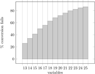
Figure 1: Failure rate of the combinatorial algorithm

The combinatorial algorithm was able to solve all input DNFs with up to five variables. But it fails on some DNFs with six variables (with the strategy to choose $a_{k+1}$ as small as possible). Our empirical analysis shows that the more variables a DNF contains the more often the conversion fails. Circa 8% of the tested DNFs with seven variables cannot be converted, for DNFs with 25 variables circa 86% cannot be converted. The failure rate for 13 to 25 variables is illustrated in Figure 1.

The linear programming algorithm was faster in direct runtime comparison, but we’re still working on improvements for the combinatorial algorithm.

As discussed in Subsec. 4.3, for the combinatorial algorithm the number of final nodes is an important criterion for its theoretical runtime. Figure 2 gives a first impression. It is hard to judge whether the growth exhibited is exponential, but in any case, the number of final nodes is much smaller than $2^{m}$: around 50000 times smaller for $m=25$.

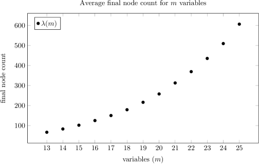
Figure 2: $\lambda(m)$ is the average number of final nodes for DNFs with $m$ variables.

6 Conclusion and future work

Linear pseudo-Boolean constraints have attracted interest because they can often be used to represent Boolean functions more compactly than CNFs or DNFs, and because techniques applied in CNF-based propositional satisfiability solving can be generalised to LPBs (?; ?).

Some Boolean functions can be represented by a single LPB. The problem of finding this LPB representation is called threshold recognition problem. In this work, we have implemented two algorithms for this problem, a classical one based on linear programming, and a more recent one that we have previously presented. The most important insight was that our algorithm is, unfortunately, incomplete.

The most important topic for future work is, of course, trying to reestablish completeness.

The obvious way to achieve this is to incorporate some kind of backtracking into the algorithm: If a DNF can be represented by an LPB and we cannot choose $a_{k+1}$, then this is because we must have chosen one of the coefficients $a_{k+2},\ldots,a_{m}$ too small, because our strategy so far was to chose the coefficients as small as possible. In order to find a solution we increment the coefficients $a_{k+2},\ldots,a_{m}$ and re-evaluate the LPBs. We can use the minimum and maximum degrees to ensure that we enumerate only legal candidates. We iteratively increment the coefficients until we can choose the coefficient $a_{k+1}$.

One problem of this approach is that for a DNF that cannot be represented by an LPB, termination is not guaranteed, because frequently the choice of the next coefficient is not bounded from above. However, we are confident that this problem can be resolved because it should be possible to derive some upper bound for each variable in the sense that it is never necessary to choose a coefficient bigger than this bound (something along the lines: it is never necessary to choose a coefficient more than $m$ times bigger than the previous coefficient).

The other problem is of course that backtracking worsens that runtime of the algorithm, and we very much fear that it will destroy the polynomial runtime of the algorithm.

The backtracking approach has been implemented and was able to find a solution for each tested input DNF. But the implementation has also shown that the higher the dimension $m$, the more often we have to use backtracking.

Alternatively, or more likely, additionally, one might use the occurrence patterns for estimating the weight ratio: In the example above we were able to represent all LPBs in the fourth column but we were not able to choose $a_{3}$ such that we can represent all LPBs in the third column with the configuration $a_{6}=1,a_{5}=a_{4}=2$. We need some global information that the distance between $a_{6}$ and $a_{5},a_{4}$ will be too small in the sequel.

Maybe it is possible to use the occurrence patterns to formulate such constraints, i.e., one might find a constraint of the form “in an LPB representing $\phi$ one has to ensure that $a_{i}\geq w\cdot a_{j}$”.

It has to be said however that there have been previous attempts to somehow directly translate the occurrence patterns into numeric coefficients or better, coefficient ratios; the threshold recognition problem has stubbornly resisted such attempts.

However, even a rough estimate of the coefficient ration, based on the occurrence patterns, might be useful for reducing if not eliminating the backtracking effort.

One other interesting topic is a more thorough analysis of the complexity of the combinatorial algorithm, whether it is in its current state or after having achieved completeness. In particular, as we have mentioned in Subsec. 4.3, analysing the effect of exploiting the symmetries in the input DNF would be interesting.

Acknowledgements

We thank Yves Crama and Utz-Uwe Haus for very fruitful discussions about this work.

References

- [Crama and Hammer 2011] Crama, Y., and Hammer, P. L. 2011. Boolean Functions - Theory, Algorithms, and Applications, volume 142 of Encyclopedia of mathematics and its applications. Cambridge University Press.
- [Dixon and Ginsberg 2000] Dixon, H. E., and Ginsberg, M. L. 2000. Combining satisfiability techniques from AI and OR. The Knowledge Engineering Review 15(1):31–45.
- [Fränzle and Herde 2007] Fränzle, M., and Herde, C. 2007. HySAT: An efficient proof engine for bounded model checking of hybrid systems. Formal Methods Syst. Des. 30(3):179–198.
- [Hooker 1992] Hooker, J. N. 1992. Generalized resolution for 0-1 linear inequalities. Ann. Math. Artif. Intell. 6(1-3):271–286.
- [Peled and Simeone 1985] Peled, U. N., and Simeone, B. 1985. Polynomial-time algorithms for regular set-covering and threshold synthesis. Discret. Appl. Math. 12(1):57–69.
- [Schilling 2011] Schilling, C. 2011. Solving the Threshold Synthesis Problem of Boolean Functions by Translation to Linear Programming. Bachelor thesis, Albert-Ludwigs-Universität Freiburg.
- [Smaus 2007a] Smaus, J. 2007a. On Boolean functions encodable as a single linear pseudo-Boolean constraint. In CPAIOR, volume 4510 of LNCS, 288–302. Springer.
- [Smaus 2007b] Smaus, J. 2007b. On Boolean functions encodable as a single linear pseudo-Boolean constraint. Technical Report 230, Institut für Informatik, Universität Freiburg. Long version of (?). Also available as TR No. 13 on www.avacs.org.
- [Wegener 1987] Wegener, I. 1987. The complexity of Boolean functions. Wiley-Teubner.
- [Wenzelmann 2011] Wenzelmann, F. 2011. Solving the Threshold Synthesis Problem of Boolean Functions by a Combinatorial Algorithm. Bachelor thesis, Albert-Ludwigs-Universität Freiburg.
- [Winder 1962] Winder, R. O. 1962. Threshold Logic. Ph.D. Dissertation, Department of Mathematics, Princeton University, Princeton, U.S.A.