Bayesian Additive Main Effects and Multiplicative Interaction Models Using Tensor Regression for Multi-environmental Trials

Abstract

We propose a Bayesian tensor regression model to accommodate the effect of multiple factors on phenotype prediction. We adopt a set of prior distributions that resolve identifiability issues that may arise between the parameters in the model. Simulation experiments show that our method out-performs previous related models and machine learning algorithms under different sample sizes and degrees of complexity. We further explore the applicability of our model by analysing real-world data related to wheat production across Ireland from 2010 to 2019. Our model performs competitively and overcomes key limitations found in other analogous approaches. Finally, we adapt a set of visualisations for the posterior distribution of the tensor effects that facilitate the identification of optimal interactions between the tensor variables whilst accounting for the uncertainty in the posterior distribution.

, , ,

1 Introduction

The phenotypic performance of a cultivar is associated with many potentially interacting variables (Hara, Piekutowska and Niedbała, 2021). These may include, but are not limited to: genetic factors; environment exposure; soil type; climatic conditions; and season. Any combinations of these factors may contribute, either positively or negatively, to the variability of the production of the crop of interest (Kross et al., 2020). Statistical modelling of the effect of these variables, both singly and jointly, is an important decision-making tool for farmers and those in the agricultural sector for predicting e.g. yield (Adisa et al., 2019).

One of the main interactions that is believed to impact most the production of a crop is the one between genotype and environment. For notational convenience, we denote such interactions as $G\times E$. This sort of interaction is characterised by cultivars that do not behave consistently in differing environments. Therefore, it is necessary to estimate the amount of variation in crop yield that is caused by the interaction. Many models have been proposed to estimate $G\times E$ (Gauch Jr, Piepho and Annicchiarico, 2008; Crossa, Vargas and Joshi, 2010; Gauch Jr, 2013). The most popular is perhaps the additive main effects and multiplicative interaction (AMMI) model (Gauch Jr, 1988), which consists of two components. The first term is the additive component, which contains the main effects of categorically structured genotype and environmental factors. The second term involves a sum of a multiplication of parameters, which are constrained to an orthonormal space and represent how strong/weak the interactions between the genotypes and environments are. To date, the models in this area have mostly been restricted to using these two sole (but important) covariates.

Our approach allows for more components beyond genotype and environment to be included in the AMMI model. We follow the Bayesian tensor regression technique of Guhaniyogi, Qamar and Dunson (2017) to allow for any number of interacting categorical factors. Tensors are algebraic structures that generalise matrices and provide a generic way of describing multidimensional arrays on a given number of axes. Tensor decomposition methods have the advantage of capturing the information in the data with a multi-linear structure and bring a unique representation without the requirement for additional constraints like sparsity or statistical independence (Jørgensen et al., 2018). The two main tensor decompositions are the PARAFAC (Carroll and Chang, 1970; Harshman et al., 1970) and Tucker models (Tucker, 1963). Tensors have been used in many fields of study, including physics (Gaillac, Pullumbi and Coudert, 2016), chemistry (Facelli, 2011), medicine (Peyrat et al., 2007), and data mining (Mørup, 2011). Guhaniyogi, Qamar and Dunson (2017) propose a tensor-based Bayesian regression model where vector/tensor covariates are used to estimate a univariate response through a class of multiway shrinkage priors. They illustrate the model on real-world data from the brain connectome as well as providing theoretical results concerning the speed at which the posterior distribution converges to the true posterior (i.e., contraction rate). Similarly, Papadogeorgou, Zhang and Dunson (2021) propose a soft tensor regression to investigate the connection between human traits and brain structural connectomics.

In this paper, we propose the Bayesian additive main effects and multiplicative interaction tensor model (BAMMIT), which generalises the AMMI model to contain a tensor of interacting terms. We extend the standard AMMI model to include new parameters to the additive and multiplicative terms of the model, taking into account factors other than genotype and environment on the phenotype of a given cultivar. Common extra factors might include soil types, replications, time points, or growth stages. We present our new model in a Bayesian hierarchical format where we place prior distributions on the main and tensor product terms so as to guarantee the model’s identifiability and impose orthonormality constraints, which are an essential part of both the original AMMI and our BAMMIT models. Our model as proposed is easily extendable to more complex dependence structures, and we explore how one such extension (time dependence) might be used in our case study.

We evaluate our proposed approach through a set of simulation experiments. Our interest is to investigate the model’s performance when the complexity increases, that is, when other variables besides genotype and environment are included and there are different sample sizes. We compare the prediction of our model with other machine learning models in terms of the root mean squared error (RMSE) and the coefficient of determination ($R^{2}$). We explore the proposed model in a real-world application where we analyse wheat data gathered across Ireland from 2010 to 2019. Again, our model demonstrates competitive performance when compared to previous approaches. Finally, we show through a new set of visualisations how the posterior distribution of the components of the BAMMIT model can be better assessed in order to quickly identify optimal interactions as well as the uncertainty associated with them.

Our paper is structured as follows. In Section 2.1, we review the AMMI model and present the constraints imposed on its two components. In Section 2.2, we introduce our BAMMIT model with its extended additive and multiplicative terms. We outline the interpretability and identifiability constraints, as well as the priors considered for the parameters and a description of obtaining the posteriors. In Section 3, we compare the results from BAMMIT with other relevant models based on synthetic data. In Section 4, we analyse a real-world application involving wheat production in Ireland. Finally, we review and discuss the findings of the work in Section 5.

2 A Bayesian AMMI Tensor (BAMMIT) Model

In this section, we review the vanilla AMMI model and define terminology and notation. We then introduce the BAMMIT model detailing the necessary constraints to ensure identifiability as well as the prior distributions and inferential scheme.

2.1 The AMMI model

The traditional AMMI model takes into account only two categorical factors, genotype and environment, and is given by a combination of two parts, one additive and one multiplicative. Let $y_{ij}$ be the outcome variable. We write the model as:

$$y_{ij}=\mu+b_{i}^{(1)}+b_{j}^{(2)}+\sum_{q=1}^{Q}\lambda_{q}\beta_{iq}^{(1)}\beta_{jq}^{(2)}+\varepsilon_{ij},\mbox{ }\varepsilon_{ij}\sim\mbox{N}(0,\sigma^{2}),$$ (1)

where $b_{i}^{(1)}$ and $b_{j}^{(2)}$ represent the marginal effect of the $i^{th}$ genotype and $j^{th}$ environment, respectively, $i=1,...,B_{1}$ and $j=1,...,B_{2}$. The bilinear term (i.e. the summation) is composed of $Q$ components, each of which having a variable $\lambda_{q}$ and the scores $\beta_{iq}^{(1)}$ and $\beta_{jq}^{(2)}$. The parameter $\lambda_{q}$ measures the interaction strength of the $q^{th}$ component and is ordered such that $\lambda_{1}\geq\lambda_{2}\geq\dots\geq\lambda_{Q}$. The scores $\beta_{iq}^{(1)}$ and $\beta_{jq}^{(2)}$ represent the importance of the $i^{th}$ genotype and the $j^{th}$ environment in the interaction. To ensure identifiability, the bilinear term is constrained so that $\sum_{i}\beta_{iq}^{(1)}\beta_{iq^{\prime}}^{(1)}=\sum_{j}\beta_{jq}^{(2)}\beta_{jq^{\prime}}^{(2)}=0$, for $q\neq q^{\prime}$ and $\sum_{i}(\beta_{iq}^{(1)})^{2}=\sum_{j}(\beta_{jq}^{(2)})^{2}=1$.

There are a range of approaches to estimating the parameters of the AMMI model. In the frequentist paradigm, the additive term of Equation (1) is estimated by ordinary least squares ignoring the interaction term, and subsequently a singular value decomposition (SVD) on the matrix of residuals is used to estimate the multiplicative terms (Gabriel, 1978). Within the Bayesian context, Viele and Srinivasan (2000) proposed the use of Markov chain Monte Carlo (MCMC) to estimate the parameters of the AMMI model ensuring that the inherent constraints of the model were not violated. Liu (2001) formulated a more stable and computationally faster Gibbs sampler. Crossa et al. (2011) and Perez-Elizalde, Jarquin and Crossa (2012) proposed a Gibbs sampler such that the algorithm was stabilised and incorporated statistical inference in the visualisation of biplots (Gabriel, 1971), drawing credibility regions for the interaction effects. By contrast, Josse et al. (2014) introduced an approach to deal with the overparametrization issue of the model by defining priors for the complete set of parameters ignoring the constraints, then applying a postprocessing on the posterior samples of each parameter. Sarti et al. (2021) used Bayesian additive regression trees (BART) in which a ‘double-grow’ BART is responsible for capturing the interaction term.

The number of terms in the summation, $Q$, is usually fixed. It is assumed that $Q\leq\mbox{min}(B_{1}-1,B_{2}-1)$. The total variability measured by the principal components is linked to the number $Q$, such that by setting $Q=\mbox{min}(B_{1}-1,B_{2}-1)$ the model can capture all the variance in the interaction. In practice, Q is commonly an integer between 1 and 3 as this allows for easier interpretation and visualisation of the interaction effects via biplots. However, many approaches can be applied to determine the value of $Q$. Examples include Cornelius (1993) who applied parametric significance tests; other authors who employed cross validation techniques (dos S. Dias and Krzanowski, 2003; Gabriel, 2002; Hadasch, Forkman and Piepho, 2017), or those using resampling techniques (Malik et al., 2018; Malik, Forkman and Piepho, 2019). Examples in the Bayesian field include Perez-Elizalde, Jarquin and Crossa (2012) and da Silva et al. (2015) where the prior choice and Bayes factor deal with determining the number of components of the multiplicative term. The non-parametric Bayesian approach of Sarti et al. (2021) bypasses the need to provide $Q$ completely but, like many BART models, suffers from interpretability problems due to the complexity of the regression trees.

One of the reasons for the popularity of the AMMI model is its strong predictive performance (Gauch Jr, 2006; Gauch Jr, Piepho and Annicchiarico, 2008), accuracy (Gauch and Moran, 2019) and its stability evaluation system (Gauch Jr, 1988; Yue et al., 2022). Given its desirable properties, many extensions can be found in the literature, as highlighted above. In this work, we aim to maintain the structure of the AMMI model and add the effects of other categorical factors that are commonly available in real-world METs.

2.2 The BAMMIT model

The model in (1) can be extended to include the effect of many factors apart from genotype and environment. Let $y_{ij\ldots v}$ be an outcome variable, in a setting with a total of $N$ observations and $V$ predictors. We define the BAMMIT model as:

$$y_{ij\ldots v}=\mu+b_{i}^{(1)}+b_{j}^{(2)}+\cdots+b_{v}^{(V)}+\sum_{q=1}^{Q}\lambda_{q}\left(\beta_{iq}^{(1)}\beta_{jq}^{(2)}\times\cdots\times\beta_{vq}^{(V)}\right)+\varepsilon_{ij\ldots v}.$$ (2)

This is similar to the AMMI model described in (1), however now we have $V$ factors instead of only two. Alternatively, we can rewrite the coefficients of the additive and multiplicative terms of (2) in tensor notation. Let $\bm{b}^{(v)}=(b_{1}^{(v)},\dots,b_{B_{v}}^{(v)})^{\top}$ be a $B_{v}$-dimensional vector of parameters of the $v^{th}$ predictor and $\bm{\beta}_{q}^{(v)}=(\beta_{1q}^{(v)},\dots,\beta_{B_{v}q}^{(v)})^{\top}$ be a $B_{v}$-dimensional vector of singular values, with $q=1,...,Q$. Binding the column vectors $\bm{\beta}_{q}^{(v)}$, we get $\bm{\beta}^{(v)}$, a matrix of dimension $B_{v}\times Q$. We define $N=\left(\prod_{v=1}^{V}B_{v}\right)$ as the total number of observations (though, for example, replication may increase $N$ without any need for extra parameters).

For notational convenience, we define a cumulative direct sum and a cumulative Kronecker product resulting in an $N$-dimensional vector as $\mathop{\vphantom{\sum}\mathchoice{\vbox{\hbox{\begin{picture}(1.0,1.0)\polygon(0.05,0.5)(0.5,0.05)(0.95,0.5)(0.5,0.95) \Line(0.5,0.05)(0.5,0.95) \Line(0.05,0.5)(0.95,0.5) \end{picture}}}}{\vbox{\hbox{\begin{picture}(1.0,1.0)\polygon(0.05,0.5)(0.5,0.05)(0.95,0.5)(0.5,0.95) \Line(0.5,0.05)(0.5,0.95) \Line(0.05,0.5)(0.95,0.5) \end{picture}}}}{\vbox{\hbox{\begin{picture}(1.0,1.0)\polygon(0.05,0.5)(0.5,0.05)(0.95,0.5)(0.5,0.95) \Line(0.5,0.05)(0.5,0.95) \Line(0.05,0.5)(0.95,0.5) \end{picture}}}}{\vbox{\hbox{\begin{picture}(1.0,1.0)\polygon(0.05,0.5)(0.5,0.05)(0.95,0.5)(0.5,0.95) \Line(0.5,0.05)(0.5,0.95) \Line(0.05,0.5)(0.95,0.5) \end{picture}}}}}\slimits@_{v=1}^{V}\mathbf{b}^{(v)}=\mathbf{b}^{(1)}{\scriptstyle\mathop{\vphantom{\sum}\mathchoice{\vbox{\hbox{\begin{picture}(1.0,1.0)\polygon(0.05,0.5)(0.5,0.05)(0.95,0.5)(0.5,0.95) \Line(0.5,0.05)(0.5,0.95) \Line(0.05,0.5)(0.95,0.5) \end{picture}}}}{\vbox{\hbox{\begin{picture}(1.0,1.0)\polygon(0.05,0.5)(0.5,0.05)(0.95,0.5)(0.5,0.95) \Line(0.5,0.05)(0.5,0.95) \Line(0.05,0.5)(0.95,0.5) \end{picture}}}}{\vbox{\hbox{\begin{picture}(1.0,1.0)\polygon(0.05,0.5)(0.5,0.05)(0.95,0.5)(0.5,0.95) \Line(0.5,0.05)(0.5,0.95) \Line(0.05,0.5)(0.95,0.5) \end{picture}}}}{\vbox{\hbox{\begin{picture}(1.0,1.0)\polygon(0.05,0.5)(0.5,0.05)(0.95,0.5)(0.5,0.95) \Line(0.5,0.05)(0.5,0.95) \Line(0.05,0.5)(0.95,0.5) \end{picture}}}}}\slimits@}\cdots{\scriptstyle\mathop{\vphantom{\sum}\mathchoice{\vbox{\hbox{\begin{picture}(1.0,1.0)\polygon(0.05,0.5)(0.5,0.05)(0.95,0.5)(0.5,0.95) \Line(0.5,0.05)(0.5,0.95) \Line(0.05,0.5)(0.95,0.5) \end{picture}}}}{\vbox{\hbox{\begin{picture}(1.0,1.0)\polygon(0.05,0.5)(0.5,0.05)(0.95,0.5)(0.5,0.95) \Line(0.5,0.05)(0.5,0.95) \Line(0.05,0.5)(0.95,0.5) \end{picture}}}}{\vbox{\hbox{\begin{picture}(1.0,1.0)\polygon(0.05,0.5)(0.5,0.05)(0.95,0.5)(0.5,0.95) \Line(0.5,0.05)(0.5,0.95) \Line(0.05,0.5)(0.95,0.5) \end{picture}}}}{\vbox{\hbox{\begin{picture}(1.0,1.0)\polygon(0.05,0.5)(0.5,0.05)(0.95,0.5)(0.5,0.95) \Line(0.5,0.05)(0.5,0.95) \Line(0.05,0.5)(0.95,0.5) \end{picture}}}}}\slimits@}\text{\hskip 2.84544pt}\bm{b}^{(V)}$ and $\bigotimes_{v=1}^{V}\bm{\beta}_{q}^{(v)}=\bm{\beta}_{q}^{(1)}\otimes\cdots\otimes\bm{\beta}_{q}^{(V)}$, respectively. The direct sum operation is defined such that for vectors $\mathbf{a}=\left(a_{1},a_{2}\right)^{\top}$ and $\mathbf{b}=\left(b_{1},b_{2},b_{3}\right)^{\top}$, for example,

$$\mathbf{a}\text{\hskip 2.84544pt}{\scriptstyle\mathop{\vphantom{\sum}\mathchoice{\vbox{\hbox{\begin{picture}(1.0,1.0)\polygon(0.05,0.5)(0.5,0.05)(0.95,0.5)(0.5,0.95) \Line(0.5,0.05)(0.5,0.95) \Line(0.05,0.5)(0.95,0.5) \end{picture}}}}{\vbox{\hbox{\begin{picture}(1.0,1.0)\polygon(0.05,0.5)(0.5,0.05)(0.95,0.5)(0.5,0.95) \Line(0.5,0.05)(0.5,0.95) \Line(0.05,0.5)(0.95,0.5) \end{picture}}}}{\vbox{\hbox{\begin{picture}(1.0,1.0)\polygon(0.05,0.5)(0.5,0.05)(0.95,0.5)(0.5,0.95) \Line(0.5,0.05)(0.5,0.95) \Line(0.05,0.5)(0.95,0.5) \end{picture}}}}{\vbox{\hbox{\begin{picture}(1.0,1.0)\polygon(0.05,0.5)(0.5,0.05)(0.95,0.5)(0.5,0.95) \Line(0.5,0.05)(0.5,0.95) \Line(0.05,0.5)(0.95,0.5) \end{picture}}}}}\slimits@}\text{\hskip 2.84544pt}\mathbf{b}=\left(a_{1}+b_{1},a_{1}+b_{2},a_{1}+b_{3},a_{2}+b_{1},a_{2}+b_{2},a_{2}+b_{3}\right)^{\top}.$$

Following the tensor notation presented, the BAMMIT model can be written more compactly as:

$$\bm{y} = \mu+\mathop{\vphantom{\sum}\mathchoice{\vbox{\hbox{\begin{picture}(1.0,1.0)\polygon(0.05,0.5)(0.5,0.05)(0.95,0.5)(0.5,0.95) \Line(0.5,0.05)(0.5,0.95) \Line(0.05,0.5)(0.95,0.5) \end{picture}}}}{\vbox{\hbox{\begin{picture}(1.0,1.0)\polygon(0.05,0.5)(0.5,0.05)(0.95,0.5)(0.5,0.95) \Line(0.5,0.05)(0.5,0.95) \Line(0.05,0.5)(0.95,0.5) \end{picture}}}}{\vbox{\hbox{\begin{picture}(1.0,1.0)\polygon(0.05,0.5)(0.5,0.05)(0.95,0.5)(0.5,0.95) \Line(0.5,0.05)(0.5,0.95) \Line(0.05,0.5)(0.95,0.5) \end{picture}}}}{\vbox{\hbox{\begin{picture}(1.0,1.0)\polygon(0.05,0.5)(0.5,0.05)(0.95,0.5)(0.5,0.95) \Line(0.5,0.05)(0.5,0.95) \Line(0.05,0.5)(0.95,0.5) \end{picture}}}}}\slimits@_{v=1}^{V}\bm{b}^{(v)}+\sum\limits_{q=1}^{Q}\lambda_{q}\left(\bigotimes_{v=1}^{V}\bm{\beta}^{(v)}_{q}\right)+\bm{\varepsilon},$$ (3)

where $\bm{y}$ is an $N$-dimensional vector, as before $\mu$ is the grand mean, $\lambda_{q}$ is the strength of the $q^{th}$ component, and $\bm{\varepsilon}$ is a noise vector such that each entry $\varepsilon_{n}\sim\mathcal{N}(0,\sigma^{2})$, with $n=1,\dots,N$. Note that each vector $\bm{b}^{(1)},\bm{b}^{(2)},\ldots,\bm{b}^{(V)}$ consists of $B_{1},B_{2},\ldots,B_{V}$ values, respectively, each of which representing the levels of a factor (e.g., 8 genotypes, 10 environments and 4 soil types would yield $B_{1}=8,B_{2}=10,B_{3}=4$, with $V=3$). The cumulative direct sum operator $\mathop{\vphantom{\sum}\mathchoice{\vbox{\hbox{\begin{picture}(1.0,1.0)\polygon(0.05,0.5)(0.5,0.05)(0.95,0.5)(0.5,0.95) \Line(0.5,0.05)(0.5,0.95) \Line(0.05,0.5)(0.95,0.5) \end{picture}}}}{\vbox{\hbox{\begin{picture}(1.0,1.0)\polygon(0.05,0.5)(0.5,0.05)(0.95,0.5)(0.5,0.95) \Line(0.5,0.05)(0.5,0.95) \Line(0.05,0.5)(0.95,0.5) \end{picture}}}}{\vbox{\hbox{\begin{picture}(1.0,1.0)\polygon(0.05,0.5)(0.5,0.05)(0.95,0.5)(0.5,0.95) \Line(0.5,0.05)(0.5,0.95) \Line(0.05,0.5)(0.95,0.5) \end{picture}}}}{\vbox{\hbox{\begin{picture}(1.0,1.0)\polygon(0.05,0.5)(0.5,0.05)(0.95,0.5)(0.5,0.95) \Line(0.5,0.05)(0.5,0.95) \Line(0.05,0.5)(0.95,0.5) \end{picture}}}}}\slimits@$ then ensures sums of main effects representing all possible combinations between levels, each corresponding to one observation in the data set. The additive term represents the individual effect of each predictor, while the summation captures via Q components the interactions between the individual effects. In the case where there is only the effect of two variables, the model in Equation 3 is reduced to the AMMI model. The summation term provides a regularisation on the complexity of the model, with larger $Q$ yielding a more complex set of interactions.

The model in the form presented in Equation (3) allows for the inclusion and study of multiple categorical predictors beyond the standard $G\times E$ pair used in AMMI models, and the understanding of their effects in two parts, individually and when interacting. As in the traditional AMMI model, $Q$ is fixed and represents how many multiplicative terms are included in the model. Common extra predictors that might be added to the model include soil type, time, or growth stages, amongst many others. Being able to tractably estimate the effect of each of these on a phenotype would be extremely useful for practitioners, whilst retaining the simple interpretation of the parameters in the AMMI model.

2.3 Prior distributions in the BAMMIT model

In order to ensure the tractability of the coefficients in the model, it is necessary to establish restrictions on both the additive and interaction terms. For the main effects term, the only constraint to be made is that the covariates are centered. For the interaction term, we note that it is not trivial to ensure the identifiability of each parameter individually, only the entire product term (Guhaniyogi, Qamar and Dunson, 2017). The constrains we use are:

1. $\bm{1}^{\prime}_{B_{1}}\bm{b}^{(1)}=\bm{1}^{\prime}_{B_{2}}\bm{b}^{(2)}=\dots=\bm{1}^{\prime}_{B_{V}}\bm{b}^{(V)}=0$.

2. $\bm{1}^{\prime}_{B_{1}}\bm{\beta}^{(1)}_{q}=\bm{1}^{\prime}_{B_{2}}\bm{\beta}^{(2)}_{q}=\dots=\bm{1}^{\prime}_{B_{V}}\bm{\beta}^{(V)}_{q}=0$.

3. ${\bm{\beta}^{(1)}}^{\prime}\bm{\beta}^{(1)}={\bm{\beta}^{(2)}}^{\prime}\bm{\beta}^{(2)}=\dots={\bm{\beta}^{(V)}}^{\prime}\bm{\beta}^{(V)}=1$.

4. $\lambda_{1}\geq\lambda_{2}\geq\dots\geq\lambda_{Q}\geq 0$.

In the Bayesian context, these constraints are ensured from the definition at the prior level. For example, in the Bayesian AMMI model proposed byPerez-Elizalde, Jarquin and Crossa (2012), the von Mises-Fisher distribution is considered for the coefficients of the multiplicative term. In the tensor field, Guhaniyogi, Qamar and Dunson (2017) introduce multiway shrinkage priors in their tensor regression model. In our approach, we provide a new method by which the constraints are met by applying the restrictions above through parameter transformations which we describe next.

Formally, we frame a hierarchical model in which prior distributions of the grand mean, main additive effects and variance parameters are

$$\mu \sim \mbox{N}(\mu_{\mu},\sigma^{2}_{\mu}),$$

$$\bm{b}^{(v)} \sim \mbox{N}(0,\sigma^{2}_{\bm{b}^{(v)}}),$$

$$\lambda_{q} \sim \mbox{N}^{+}(0,\sigma^{2}_{\lambda}),$$

$$\sigma^{-2}_{y} \sim \mbox{G}(a_{0},a_{1}),$$

$$\sigma_{\bm{b}^{(v)}} \sim \mbox{t}^{+}(0,a_{2}),$$

$$\sigma_{\lambda} \sim \mbox{t}^{+}(0,a_{3}),$$

where N, $\mbox{N}^{+}$, G, and $\mbox{t}^{+}$ are the Normal, truncated Normal, Gamma, and truncated $t$-Student distributions, respectively. The hyperparameters of the grand mean $\mu_{\mu}$ and $\sigma^{2}_{\mu}$ are fixed as are all $a_{k}$ terms, with k = 1, …, 3. We treat the additive effects as random and so estimate $\sigma_{\bm{b}^{(v)}}$, though a ‘fixed effects’ version could also be obtained. We express the prior knowledge on the standard deviations of the additive term parameters and the $\lambda$ parameter using a truncated $t$ distribution. Additionally, we impose that the estimated $\bm{\lambda}$ vector values are in descending order.

For the product parameters in the interaction term, we use a transformation to ensure the constraints are met. Specifically, we generate an auxiliary variable $\theta_{\beta^{(v)}_{iq}}$ from a standard $\mathcal{N}(0,1)$ distribution (the transformation is invariant to the scale of this distribution), with $i=1,\dots,B_{v}$, $v=1,...,V$, $q=1,,\dots,Q$. Then, we centre by the mean $\mu_{\bm{\beta}^{(v)}_{q}}$ of the vector $\bm{\beta}^{(v)}_{q}$, that is, for each vector $\bm{\beta}^{(v)}_{q}$ we calculate its mean and then subtract it from the auxiliary variable $\theta_{\beta^{(v)}_{iq}}$ for the respective value of q. Finally, we get the final $\beta^{(v)}_{iq}$ value via:

$$\beta^{(v)}_{iq} = \left(\theta_{\beta^{(v)}_{iq}}-\mu_{\bm{\beta}^{(v)}_{q}}\right)\left[\sum_{i}\left(\theta_{\beta^{(v)}_{iq}}-\mu_{\bm{\beta}^{(v)}_{q}}\right)^{2}\right]^{-1/2}.$$

Applying this procedure to the parameters of the matrix $\bm{\beta}^{(v)}$ guarantees that the identifiability constraints (2) and (3) of the model are met in the inferential process.

3 Simulation

To evaluate the performance of the BAMMIT model, we simulate data from Equation (3) over a grid of $V=2,3,4$, where $B_{v}$ is constructed to allow for differences in the interaction structures. We set up the simulation experiments as follows:

• $V=2$ and $N=120$, with $B_{1}=12$, $B_{2}=10$;

• $V=3$ and $N=480$, with $B_{1}=12$, $B_{2}=10$, $B_{3}=4$;

• $V=4$ and $N=960$, with $B_{1}=12$, $B_{2}=10$, $B_{3}=4$, $B_{4}=2$;

• $V=3$ and $N=5000$, with $B_{1}=100$, $B_{2}=10$ and $B_{3}=5$.

Our goal with the above scenarios is to explore the performance of the BAMMIT model in situations where the AMMI model can be applied (case i) and situations where the number of genotypes/environments is small, medium and large. Scenarios (ii) and (iii) present a challenge to the classic AMMI model because it cannot be applied directly. Together, scenarios (i), (ii) and (iii) evaluate our model’s performance when the number of predictors increases. Finally, scenario (iv) presents a computationally challenging scenario for BAMMIT as it involves a large number of observations.

For each of these scenarios we set the real number of terms $Q_{sim}=\{1,2,3\}$ taking $\lambda=\{\{10\},\{8,10\},\{8,10,12\}\}$. We simulated 12 training and 12 test data sets. In other words, in scenario (i) there are two predictors and 120 observations, setting 12 values for the first predictor and 10 for the second. Given these number of observations and variables, we generate three data sets, one where the value of $Q_{sim}=1$ and $\lambda=10$, another where $Q_{sim}=2$ and $\lambda$ is defined as 8 and 10, and finally, a data set in which $Q_{sim}=3$ and $\lambda$ takes the values 8, 10 and 12. The same understanding extends to the other cases. In all scenarios, we set $\mu=100$, and $\sigma^{2}=1$.

To fit the BAMMIT model, we run a Markov chain Monte Carlo (MCMC) algorithm through the probabilistic programming language Just Another Gibbs Sampler (JAGS; Plummer et al., 2003) and the R package R2jags (Su and Yajima, 2021). We set $Q=\{1,2,3\}$ as the true number of components, $\mu_{\mu}=100$, $\sigma^{2}_{\mu}=10$, $a_{0}=a_{1}=0.1$, and $a_{2}=a_{3}=1$. We use three chains, 4000 iterations per chain, discarding the first 2000 as burn-in, and a thinning rate of two. Regarding computational time, a data set with three predictors ($V=3$), $N=100$ and $Q=1$ takes on average one minute to run, whilst to run a data set with $N=1000$ takes 30 minutes, and with $N=5000$, it takes on average 6 hours. We discuss computational issues further in Section 5. All experiments were implemented in R, and the code used is available at https://github.com/Alessandra23/bammit.

To assess the performance of the model when $V>2$, we compare BAMMIT with two models extensively employed for prediction purposes, namely Random Forests (RF) and eXtreme Gradient Boosting (XGB). We also compare with the traditional AMMI and AMBARTI model (Sarti et al., 2021), though these are unavoidably restricted to using only the first two variables. For the RF model, we use the package randomForest (Liaw et al., 2002) selecting the default settings, mtry$=2$ and 500 trees. For the XGB model, we use the package xgboost (Chen et al., 2019) setting 50 iterations. For the AMBARTI model we use the package AMBARTI setting 50 trees, 500 as burn-in and 1000 iterations as post burn-in. All the models were fitted to the training data. We checked the accuracy, using the test data, by comparing the posterior mean estimates with the true parameter values used in the simulations. We use the root mean squared error (RMSE) to measure predictive power (how close $\hat{y}$ is to the true $y$) and $R^{2}$ to assess the proportion of explained variability.

3.1 Simulation results

The scatterplot in Figure 1 shows this comparison of the additive portion of Equation (3), taking $V=4$, $Q_{sim}=2$, $N=960$ when the true value of $\lambda=\{8,10\}$. Each point is an estimated level of the parameter and the error bars are the $90\%$ credible intervals. By visual inspection, the estimates of the effects of the four main predictors are close to the true values, with narrower intervals for predictors with a greater number of levels.

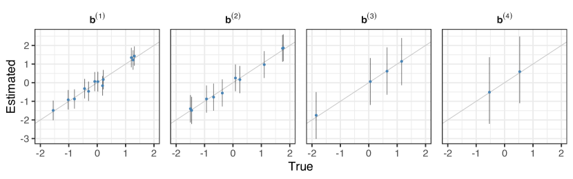
Figure 1: Scatterplots of true versus estimated additive term for simulation scenario (iii), setting $Q_{sim}=2$, $\lambda=\{8,10\}$. The bars represent the $90\%$ credible interval.

In Figure 2, we compare the estimates against the true values in the case where the number of predictors varies. Each point represents an interaction term estimate in a total of 120 ($V=2$), 480 ($V=3$) and 960 ($V=4$) points, and the bars, again, represent the $90\%$ credible intervals. We observe that when $V=4$, the dispersion is smaller and the interaction estimates are more concentrated around zero. This can be explained because as more predictors are added to the additive term of the model, the greater the approximation of the response by the predictors and the smaller the amount approximated by the interaction term, despite inserting more variables in both terms of the model. Also, note that the interaction is comprised of all the new variables together, and that this interaction may not be that strong. For example, suppose we are looking at the genotype $\times$ environment $\times$ soil type $\times$ growth stage interaction. In this case, the interaction of the four factors together is not as strong as if we were looking only at subsets of these interactions, such as genotype $\times$ environment $\times$ growth stage.

.

Figure 2: Scatterplots of true versus estimated interaction terms for simulations scenarios (i), (ii) and (iii) setting $Q_{sim}=1$ and $\lambda=10$. The bars represent the $90\%$ credible intervals.

To investigate how much the estimation of the interaction term is influenced by the choice of the value of $Q$, we study the case when the data are simulated with $Q_{sim}=2$ and $V=3$, but the number of components in the model fit is $Q=\{1,2,3\}$. The fixed value in the simulation was determined because, in real-world applications, the true number of terms in the interaction is not known. Thus we wanted to compare the behaviour of the model in a situation where we know the true value of $Q$ in the data, though it is of course fixed in the model. Figure 3 shows the $90\%$ credible error bars solely for the interaction term. As expected, the performance of the model setting $Q=3$ is better since there is an increase in the complexity of the model fit to match the data. When $Q$ is set too small, as in the left panel, we see the model being unable to capture the interaction terms. However, when the value of $Q$ used in the model fit is at least as big as the value used in the simulation, we obtain superior results.

In terms of predictions, Table 1 shows the prediction RMSE and the $R^{2}$ considering the cases where we have three and four predictors in the models (simulation scenarios (ii) and (iii)). To fit BAMMIT and AMMI models we used $Q=2$. As stated above, the AMBARTI and AMMI models were fitted disregarding the effects of the other variables. Specifically, in scenario (iii), for example, there were three predictors, but the two aforementioned models disregarded the effect of the third predictor. The BAMMIT model clearly performed better than the other two models. In addition to the prediction advantage, our model stands out from RF and XGB as it can accommodate the interaction between variables, while at the same time providing estimates based on posterior distributions. Another highlight is that BAMMIT is able to satisfactorily explain the variability of the response variable, since the $R^{2}$ obtained in all scenarios was above 75%. In a real world scenario where the data were not simulated from the BAMMIT model we might expect that the machine learning approaches would be more competitive in terms of their performance. However they would still not allow for clear interpretation of the interaction effects.

V = 3 V = 4 BAMMIT AMBARTI AMMI RF XGB BAMMIT AMBARTI AMMI RF XGB RMSE 0.92 2.54 2.52 1.68 1.26 0.96 2.74 2.71 1.74 1.15 $R^{2}$ 0.78 0.02 0.02 0.58 0.69 0.81 0.01 0.01 0.68 0.78

Table 1: RMSE and $R^{2}$ for $\hat{y}$ on out-of-sample data for scenarios (ii) and (iii).

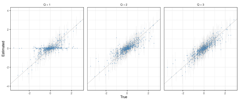
Figure 3: Scatterplots of true versus estimated interaction term for a simulation scenario setting $N=480$, $Q_{sim}=2$, $\lambda=\{8,10\}$. Each plot is a result of the Bayesian fit for three possible values of $Q$ ($1,2,3$). The bars represent the $90\%$ credible interval.

4 Case Study

In this section, we investigate the performance of the model on a real data set. The data was collected over ten years (2010 – 2019) and concerns the production of a common species of wheat (Triticum aestivum L.) in Ireland, with the response being the yield of wheat measured in tonnes per hectare (t/ha). The data comes from the Horizon2020 EU InnoVar project (www.h2020innovar.eu) and was supplied by the Irish Department of Agriculture, Food and the Marine. The experiments were conducted using a randomised complete block design with four replicates. The data set contains 85 genotypes and 17 environments, all anonymised and named as $g_{1},\dots,g_{85}$ and $e_{1},\dots,e_{17}$, respectively. Owing to not all genotypes being observed in each location in all seasons, the total number of observations genotype $\times$ location $\times$ year $\times$ block is 6,368, rather than 14,450. An advantage of the BAMMIT model is that we are able to impute the missing combinations as part of the model fit.

A subsample of this data was previously explored by Sarti et al. (2021), considering only two factors: genotype and environment. However, in our work, we include the additional variables year and block, present in the Irish data set, as a third and fourth effect in the BAMMIT model. We expect to detect if the year is an important predictor in the models, as affirmed by Hara, Piekutowska and Niedbała (2021) that the ability to predict the yield in a certain year can be useful for making decisions, such as cultivation planning and storage.

We are interested in answering some specific questions. Initially, when fixing the year and block effect, we would like to know which genotype has the best performance, in which environment, and also which environment provides the highest yield. When considering all the variables, we investigated which year and block had the best performance. One of the main tasks is to understand how accurate our predictions are and to examine the uncertainty associated with the answers from the previous questions. As an extension to the model, we include additional structure to the time component of the model by adding autoregressive terms in year.

4.1 Autoregressive structure on the time predictor (AR-BAMMIT)

In this particular application, where one of the variables in the BAMMIT model is the year of production, we have the option of extending the model by applying a different structure to the time predictor in both terms, that is, additive and multiplicative. The model is now:

$$y_{ijtr} = \mu+b^{(1)}_{i}+b^{(2)}_{j}+b^{(3)}_{t}+b^{(4)}_{r}+\sum\limits_{q=1}^{Q}\lambda_{q}\beta^{(1)}_{iq}\beta^{(2)}_{jiq}\beta^{(3)}_{tq}\beta^{(4)}_{rq}+\epsilon_{ijtr},$$ (4)

$$b^{(3)}_{t} = \alpha_{b}+\phi_{b}b^{(3)}_{t-1}+\eta_{t},$$ (5)

$$\theta^{(3)}_{tq} = \alpha_{\theta}+\phi_{\theta}\theta^{(3)}_{(t-1)q}+\omega_{t},$$ (6)

$$\beta^{(3)}_{tq} = \left(\theta^{(3)}_{tq}-\mu_{\theta^{(3)}_{q}}\right)\left[\sum_{t}(\theta^{(3)}_{tq}-\mu_{\theta^{(3)}_{q}})^{2}\right]^{-1/2},$$ (7)

where the indexes $i,j,t$ and $r$ are associated to genotypic, environmental, time and block effects, respectively. The priors for the entire model follow the same structure as before, such that Equation (7) is defined to meet the conditions of identifiability of the model. To estimate the autoregressive parameters $\phi_{b}$ and $\phi_{\theta}$ we use uniform priors in the interval $[-1,1]$. A normal distribution with mean zero and variance 100 was considered for the parameters $\alpha_{b}$ and $\alpha_{\theta}$. The priors for $\eta_{t}$ and $\omega_{t}$ were a truncated $t$-Student distribution with parameters zero and one. More details about the model structure are given in Appendix B.

4.2 Results

To fit the BAMMIT model we selected two replicates randomly for training and the last two for validation, in a total of 3,184 observations in each data set. Therefore, we have $V=4$, $B_{1}=85$ genotypes, $B_{2}=17$ environments, $B_{3}=10$ years and $B_{4}=2$ block effects. Assuming there is little information to establish the hyperparameters for our priors, we set $\mu_{\mu}=10$, $\sigma^{2}_{\mu}=1$, obtained from the mean and the standard deviation of the data, $a_{0}=a_{1}=0.1$, and $a_{2}=a_{3}=1$. To input the number of $Q$ terms, we run the model with $Q=1,2,3$. The model is fitted with three Markov chains, 4,000 iterations per chain, discarding 2,000 and a thinning rate of two.

We compare our BAMMIT approach with traditional AMMI and AMBARTI models. In addition, we fit the AR-BAMMIT model, following Equations (5) to (7). For the AMBARTI model, we considered 50 trees, 1000 iterations as burn-in and 1000 iterations as post burn-in. To assess the performance of the predictions $\hat{y}$, we display the RMSE and the $R^{2}$ in Table 2 for each model. As the AMBARTI and classic AMMI models can only handle the genotype and environment variables, we performed two procedures to treat the training and test data sets. The first takes into account all rows in the data set and ignores the year and block variables, so that rows corresponding to the same genotype and the same environment are treated as different (columns AMBARTI ALL YEARS and AMMI ALL YEARS in Table 2). In the second approach, the data set are separated by years, so that for each year we run the model. Then, we regroup the estimates obtained for each group of years, having a single data set, and calculate the metrics (AMBARTI BY YEAR and AMMI BY YEAR columns in the table). The results presented in the table were observed considering Q = 1 for the BAMMIT, AR-BAMMIT and AMMI models (ALL YEARS and BY YEAR).

	BAMMIT	AR-BAMMIT	AMBARTI BY YEAR	AMBARTI ALL YEARS	AMMI BY YEAR	AMMI ALL YEARS
RMSE	0.68	0.68	0.59	1.66	0.66	1.60
$R^{2}$	0.88	0.89	0.91	0.34	0.88	0.38

Table 2: Metrics for out-of-sample $y$ for different models. ALL YEARS refers to the fact that the model took into account all rows of the data set and ignored the year and the block variables effect. BY YEAR means that the data set was separated by years and the model was run for each group.

The results presented in Table 2 show that the AMBARTI and AMMI models were superior to BAMMIT in terms of prediction when the data set is separated by year. However, when all the years are together, these models performed poorly. For the AMBARTI, these results can be explained by the high numbers of genotypes and environments. As mentioned above, considering all the 10 years, there are 85 genotypes and 17 environments, and this case the AMBARTI model is not efficient in the generation of the $2^{B_{1}-1}-1$ and $2^{B_{2}-1}-1$ 2-partition combinations for genotypes and environments. Thus, due to the high numbers of possible combinations, the interaction component of the AMBARTI model is not able to estimate the interactions between genotypes and environments efficiently and the model performs poorly. Also, the inferior performance of classic AMMI model and AMBARTI was expected, since the adjusted models do not take into account the effects of the other variables. It is Interesting to note that, for the BAMMIT model, the best RMSE was obtained by setting $Q=1$ in the model fit, since when $Q=2$ and $Q=3$ the RMSE was 0.69 and 0.71 respectively.

4.3 Posterior visualisation

A common way to visualise the genotype and environment interactions in an AMMI model is through biplots (Gabriel, 1971). However, Sarti et al. (2021) used a heatmap to visualise the predictions and interactions. In this visualisation approach, it is possible to identify in a more immediate way the best interactions between genotypes and environments. A shortcoming of their approach concerns the quantification of uncertainty, which cannot be observed directly on the graph. To address this particular issue, in this work we show the prediction for interactions through a heatmap as in Sarti et al. (2021) and the uncertainty is showed as Value-suppressing uncertainty palettes (VSUP) as presented by Inglis, Parnell and Hurley (2022).

First introduced by Correll, Moritz and Heer (2018) value-suppressing uncertainty palettes are bivariate colour palettes that represent a measure or value and its uncertainty. The outputs for each combination of value and uncertainty in traditional bivariate palettes are often shown as a 2D square (for example see, Robertson and O’Callaghan (1986)), However, VSUP plots combine cells in the palette using a tree structure to suppress the measure or value at higher levels of uncertainty. In VSUP, when the uncertainty is low, more bins are allocated to the colour space. When increasing in uncertainty, the values are suppressed into fewer bins that blend together their colour value. By doing this, the values will become more distinct as the level of uncertainty reduces, with the intention of making it easier to detect the difference between low and high uncertainty.

In Figure 4 we display an ordered heatmap and VSUP legend for the Irish data selecting the year 2015 in block three from the test data set. This year corresponds to the best average wheat production observed in the data. The remaining years are shown in Appendix A. For these plots we use the standard deviation of the predictions as our measure of uncertainty and the value shown is the median prediction for each variable pair. The plots are ordered so that generally high predicted yield values are pushed to the top left of the plot and descend to the bottom right. The environments $e_{2}$, $e_{9}$, $e_{11}$ and $e_{16}$ were the worst environments observed, having a small median value compared to the others. On the other hand, environment $e_{1}$ was the best and most stable, presenting a median yield value higher than the others and a lower uncertainty. The environment $e_{6}$ had a middling production across some genotypes, but with a higher uncertainty when compared to the others. Applying the same interpretation to the genotypes, we observed that the genotypes $g_{3}$, $g_{26}$ and $g_{85}$ had the best performance. The genotypes $g_{17}$ and $g_{20}$ presented a good production of predicted wheat on environment $e_{1}$, $e_{5}$ and $e_{7}$, however with a higher standard deviation than the other genotypes, which also produced around 14 t/ha in this environment. The worst genotype $\times$ environment combinations observed were $e_{9}\times g_{81}$, $e_{2}\times g_{81}$, $e_{2}\times g_{71}$, $e_{2}\times g_{62}$, $e_{2}\times g_{48}$ and $e_{2}\times g_{15}$, while the best were $e_{1}\times g_{85}$, $e_{1}\times g_{30}$, $e_{1}\times g_{26}$ and $e_{1}\times g_{3}$. The results are comparable to those of Sarti et al. (2021).

In Figure 5 we plot the median yield by year. We can see that the best production occurred in the years 2015 to 2017, with the first having a smaller variation than the others. Another important factor to observe is the effect of interaction, especially related to the genotype effect. Yan et al. (2000) affirms that in multi-environment trials (MET), the primary source of interest in the evaluation of the genotypes is via the genotype effect plus $g\times e$ interaction. This enables plant breeders to determine not only those genotypes with optimal performance but also evaluate variability across environments. In Figure 6 we present the interaction effect added to the individual genotype effect. As in Figure 4, the graph is oriented downwards, that is, high values of the sum $(genotype+genotype\times environment)$ at the top and low values at the bottom. We observe that genotype $g_{3}$ is optimal in having a generally high performance score whilst also being stable across environments. .

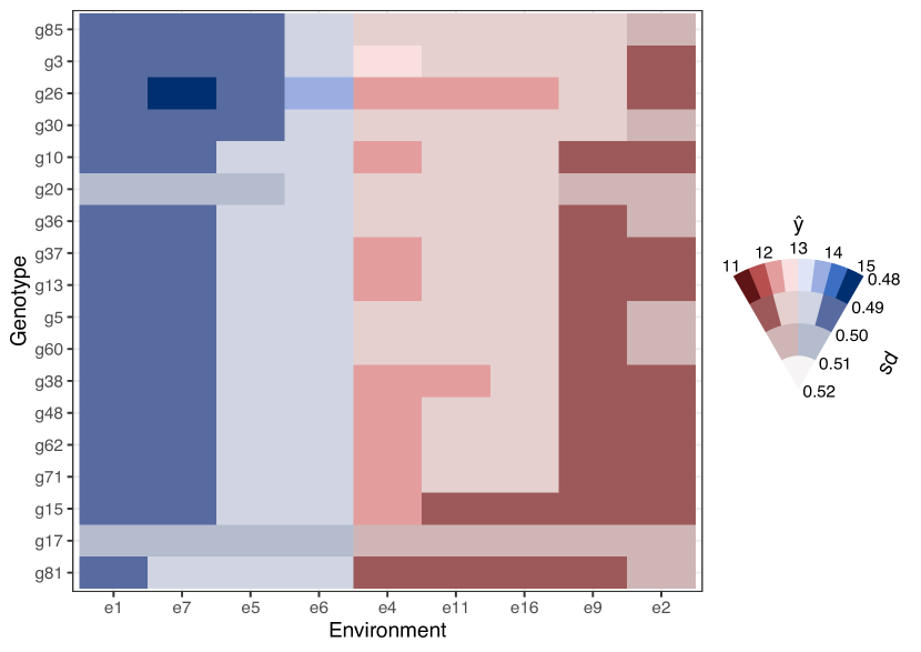
Figure 4: Predicted yields from the BAMMIT model for the data set in 2015. Production this year was high, between 11 and 15 tonnes per hectare, with positive emphasis on the environment $e_{1}$, the genotype $g_{26}$ and on the combination $g_{26}\times e_{7}$.

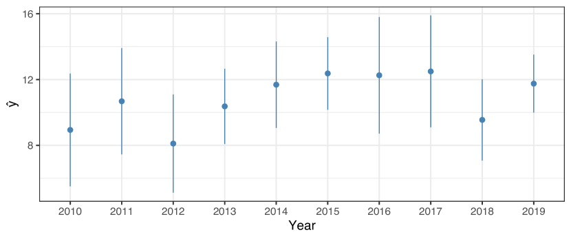
Figure 5: Median yield by year. The bars are the $\hat{y}$ plus two times the standard deviation.

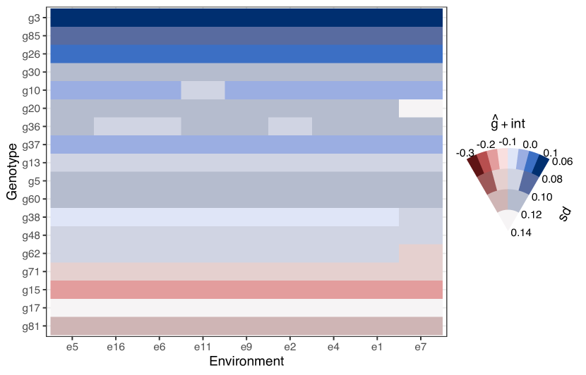
Figure 6: Predicted addiction of genotype and interaction from the BAMMIT model for the data set in 2015.

5 Discussion

In this paper, we propose a generalisation of the AMMI model which uses the tensor regression approach of Guhaniyogi, Qamar and Dunson (2017) and Papadogeorgou, Zhang and Dunson (2021) to extend the model to allow for multiple interacting categorical variables. The main idea is to allow for more realistic understanding of phenotypic effects beyond the usually considered pair of genotype and environment. We envisage that in the future such models may be used to further indicate interactions between season, soil, weather conditions, growth stage and other potential predictors. The priors we use on the hierarchical model were built in order to meet the restrictions imposed on the model and to ensure identifiability. For each simulated data set and for the estimates obtained from the Bayesian fit, the constraints were checked.

In the simulation results, the model displayed promising performance, in the sense that the estimates corresponded with the true values of the parameters from the simulation. As expected, when the established number of terms in the interaction is three, the Bayesian model had a better fit, regardless of the true number used in the simulation. The choice of the number of components $Q$ is still arbitrary, taking into account only the typical values already mentioned in the literature. Nonetheless, a more sophisticated approach to choosing the rank $Q$ can be applied, as shown by Guhaniyogi, Qamar and Dunson (2017).

When the model was applied to the real data, it was possible to establish which genotypes, environments, blocks and years had the highest wheat production. Also, we could visualise just the interaction effect and so it was possible to determine the optimal interactions. The purpose of showing the results in the visualisations presented in this paper is to aid a researcher’s ability to interpret the results and improve recommendations. Although the AMBARTI model had a superior result in relation to BAMMIT, it performed well, even with a small number of interaction terms. When compared with the Bayesian AMMI model, both BAMMIT and AR-BAMMIT were superior in terms of prediction.

In relation to the computational time, the cost for the method was high, especially when the number of components $Q$ increased; when setting $Q=3$ it took eight hours to complete the fit. This drawback was true in general when the size of the data set was large (around 5,000 total observations or more) with the model taking hours to form a valid posterior distribution. In future work, we could be use faster computational methods such as variational inference (Blei, Kucukelbir and McAuliffe, 2017; Dos Santos et al., 2022) or those as discussed in Papadogeorgou, Zhang and Dunson (2021) and Zhang et al. (2020).

As we have seen, there is an obvious extension of these models through the prior distributions. New structures can be added to certain predictors, as was done here for the year variable in the data set. Any temporal and spatial components could have their inherent characteristics inserted in the model. Another important point is the insertion of continuous variables, or latent representations of them, since the current structure does not allow for this type of variable.

[Acknowledgments] Antônia A. L. dos Santos, Andrew Parnell, and Danilo Sarti received funding for their work from the European Union’s Horizon 2020 research and innovation programme under grant agreement No 818144. In addition Andrew Parnell’s work was supported by: a Science Foundation Ireland Career Development Award (17/CDA/4695); an investigator award (16/IA/4520); a Marine Research Programme funded by the Irish Government, co-financed by the European Regional Development Fund (Grant-Aid Agreement No. PBA/CC/18/01); SFI Centre for Research Training in Foundations of Data Science 18/CRT/6049, and SFI Research Centre awards I-Form 16/RC/3872 and Insight 12/RC/2289_P2. For the purpose of Open Access, the author has applied a CC BY public copyright licence to any Author Accepted Manuscript version arising from this submission.

Appendix A Additional results

In this section, we complement the results presented in the Section 4. Figure 8 presents the graphs for the predicted yields for the BAMMIT model applied to the Irish time series data set (except year 2015). Analysing only the legend of the figures and looking at the value scale it is possible to see that the forecast of wheat yield for the year 2015 (presented in Figure 4) was higher than that for all the other years. In order to clearly observe the behaviour of genotype and environment predictors in each year, we do not scale the estimated value and the uncertainty legend to be equal across plots. Thus, we prevent years with high production and low uncertainty having an intense colour while years with contrary behaviour have a washed-out colour.

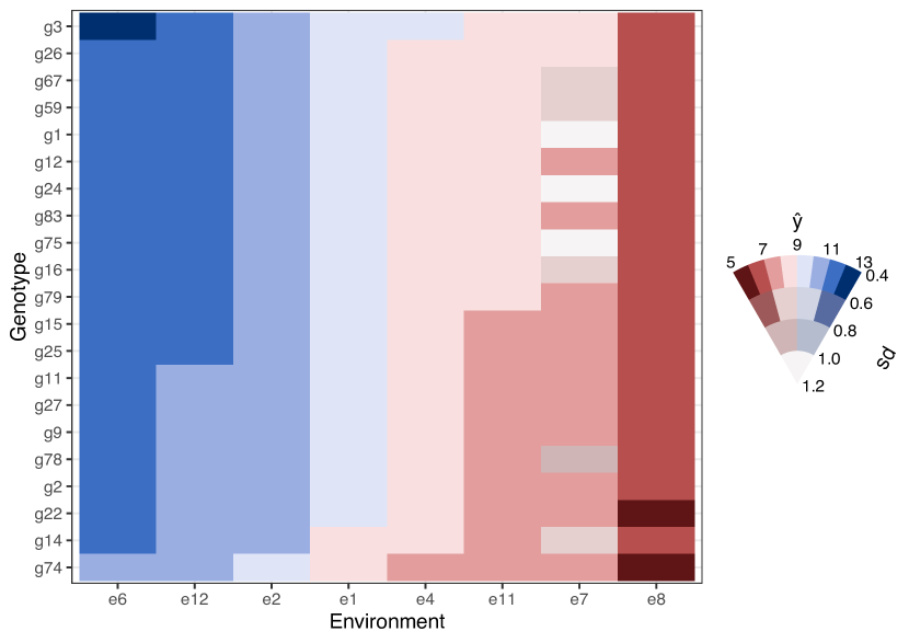
(a) 2010

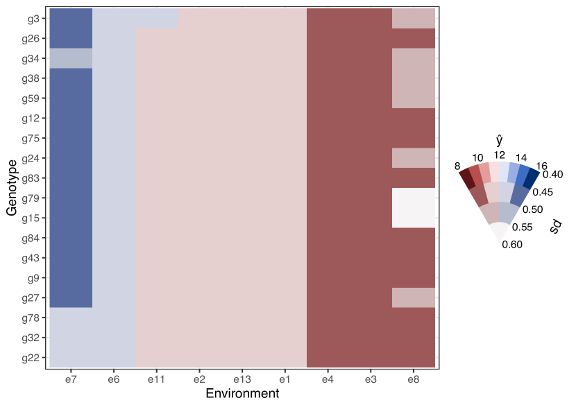
(b) 2011

Figure 7: Predicted yields from the BAMMIT model for the Irish data set.

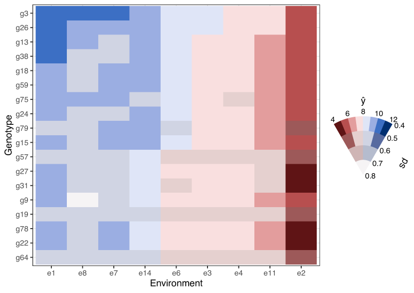
(a) 2012

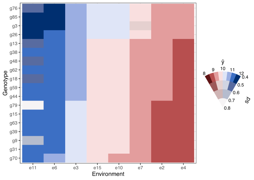
(b) 2013

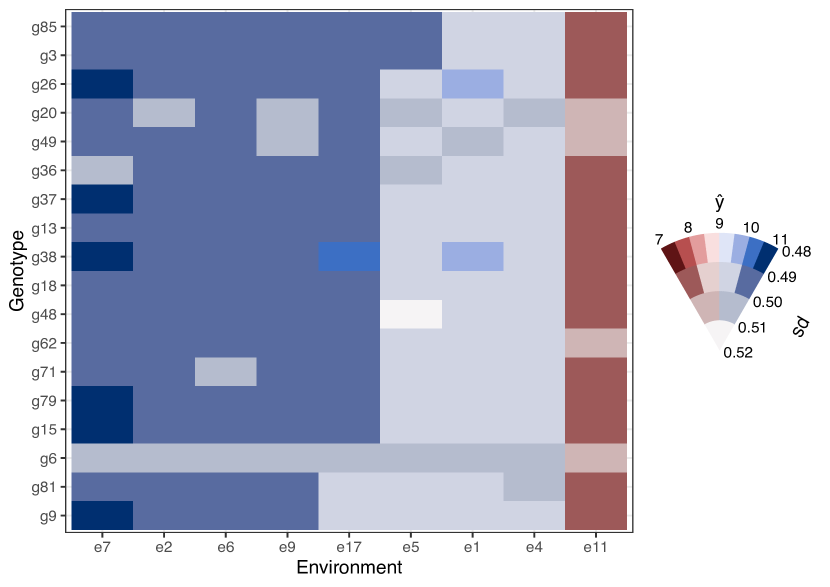
(c) 2014

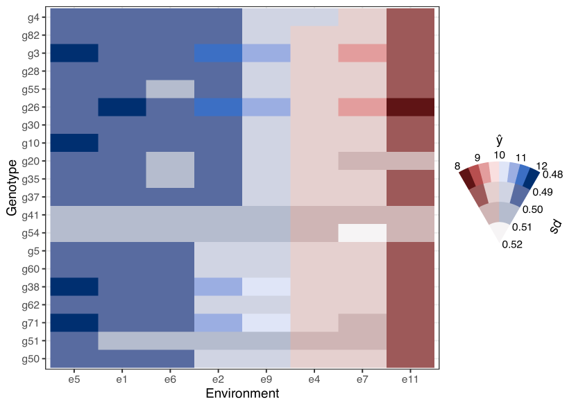
(d) 2016

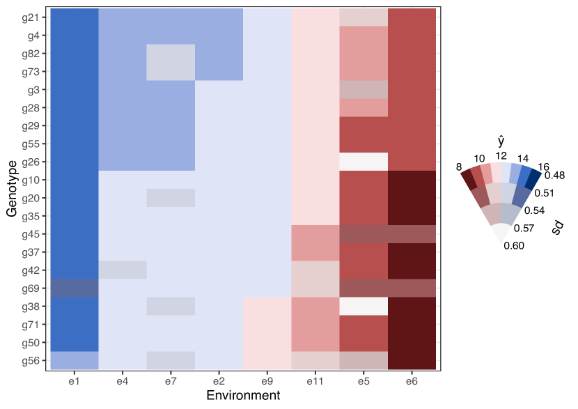
(e) 2017

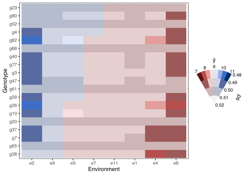
(f) 2018

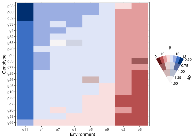
(g) 2019

Figure 8: Predicted yields from the BAMMIT model for the Irish data set on block three.

Appendix B Study of AR-BAMMIT model

The construction of the BAMMIT model allows new structures to be applied to the parameters, such as spatial or temporal. However, the insertion of these new structures brings greater complexity to the model, since it is necessary that the restrictions continue to be guaranteed. In Section 4.1, a temporal architecture is applied to the parameters associated with years in the Equation 3. In this section, we intend to explore the aforementioned AR-BAMMIT method (Section 4.1) by carrying out a small simulation study. To ensure the needed restrictions, we apply the transformation made earlier in Section 2.3 to the parameters of the interaction term also to the parameters of the new model structure.

The simulation scenarios considered were scenarios (ii) and (iii) of Section 3, where only one of the variables in the additive term and one variable in the multiplicative term have the autoregressive structure. In Figure 9, we present the scatterplot of the true and estimated main effects values for the simulation scenario (ii). Figure 10 shows the posterior density of the precision parameter and a scatterplot of the interaction term in this scenario.

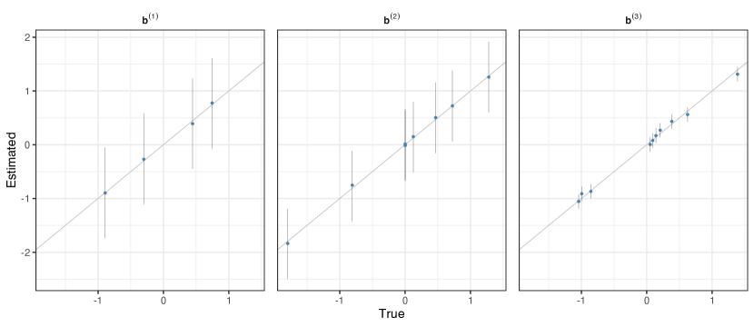
Figure 9: Posterior density for the years and for the first four genotypes and environments, setting $V=3$, $N=480$, $B_{1}=8$, $B_{2}=4$, $B_{3}=10$, $Q_{sim}=1$, $\lambda=12$.

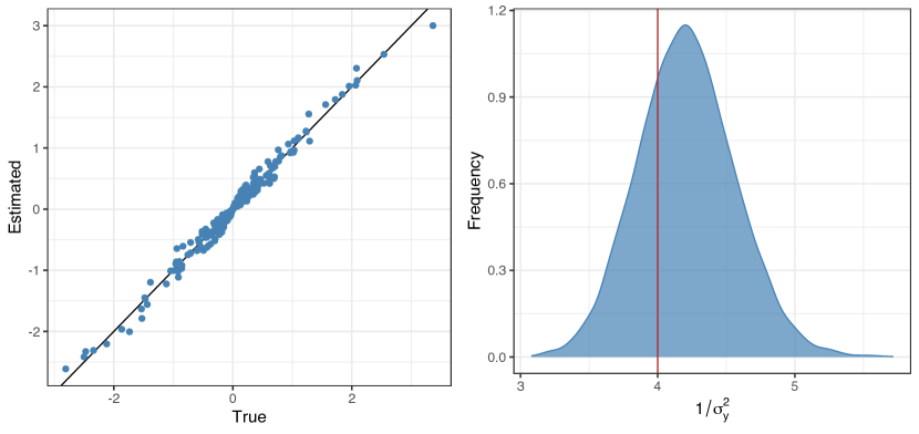
Figure 10: Scatterplot of the interaction term and the posterior distribution of the precision parameter for the simulation scenario (ii). The red line corresponds to the true value of the parameter.

References

- Adisa et al. (2019) {barticle}[author] \bauthor\bsnmAdisa, \bfnmOmolola M\binitsO. M., \bauthor\bsnmBotai, \bfnmJoel O\binitsJ. O., \bauthor\bsnmAdeola, \bfnmAbiodun M\binitsA. M., \bauthor\bsnmHassen, \bfnmAbubeker\binitsA., \bauthor\bsnmBotai, \bfnmChristina M\binitsC. M., \bauthor\bsnmDarkey, \bfnmDaniel\binitsD. and \bauthor\bsnmTesfamariam, \bfnmEyob\binitsE. (\byear2019). \btitleApplication of artificial neural network for predicting maize production in South Africa. \bjournalSustainability \bvolume11 \bpages1145. \endbibitem
- Blei, Kucukelbir and McAuliffe (2017) {barticle}[author] \bauthor\bsnmBlei, \bfnmDavid M\binitsD. M., \bauthor\bsnmKucukelbir, \bfnmAlp\binitsA. and \bauthor\bsnmMcAuliffe, \bfnmJon D\binitsJ. D. (\byear2017). \btitleVariational inference: A review for statisticians. \bjournalJournal of the American statistical Association \bvolume112 \bpages859–877. \endbibitem
- Carroll and Chang (1970) {barticle}[author] \bauthor\bsnmCarroll, \bfnmJ Douglas\binitsJ. D. and \bauthor\bsnmChang, \bfnmJih-Jie\binitsJ.-J. (\byear1970). \btitleAnalysis of individual differences in multidimensional scaling via an N-way generalization of “Eckart-Young” decomposition. \bjournalPsychometrika \bvolume35 \bpages283–319. \endbibitem
- Chen et al. (2019) {barticle}[author] \bauthor\bsnmChen, \bfnmTianqi\binitsT., \bauthor\bsnmHe, \bfnmTong\binitsT., \bauthor\bsnmBenesty, \bfnmMichael\binitsM. and \bauthor\bsnmKhotilovich, \bfnmVadim\binitsV. (\byear2019). \btitlePackage ‘xgboost’. \bjournalR version \bvolume90 \bpages1–66. \endbibitem
- Cornelius (1993) {barticle}[author] \bauthor\bsnmCornelius, \bfnmPL\binitsP. (\byear1993). \btitleStatistical tests and retention of terms in the additive main effects and multiplicative interaction model for cultivar trials. \bjournalCrop science \bvolume33 \bpages1186–1193. \endbibitem
- Correll, Moritz and Heer (2018) {binproceedings}[author] \bauthor\bsnmCorrell, \bfnmMichael\binitsM., \bauthor\bsnmMoritz, \bfnmDominik\binitsD. and \bauthor\bsnmHeer, \bfnmJeffrey\binitsJ. (\byear2018). \btitleValue-suppressing uncertainty palettes. In \bbooktitleProceedings of the 2018 CHI Conference on Human Factors in Computing Systems \bpages1–11. \endbibitem
- Crossa, Vargas and Joshi (2010) {barticle}[author] \bauthor\bsnmCrossa, \bfnmJose\binitsJ., \bauthor\bsnmVargas, \bfnmMateo\binitsM. and \bauthor\bsnmJoshi, \bfnmArun Kumar\binitsA. K. (\byear2010). \btitleLinear, bilinear, and linear-bilinear fixed and mixed models for analyzing genotype environment interaction in plant breeding and agronomy. \bjournalCanadian Journal of Plant Science \bvolume90 \bpages561–574. \endbibitem
- Crossa et al. (2011) {barticle}[author] \bauthor\bsnmCrossa, \bfnmJosé\binitsJ., \bauthor\bsnmPerez-Elizalde, \bfnmSergio\binitsS., \bauthor\bsnmJarquin, \bfnmDiego\binitsD., \bauthor\bsnmCotes, \bfnmJosé Miguel\binitsJ. M., \bauthor\bsnmViele, \bfnmKert\binitsK., \bauthor\bsnmLiu, \bfnmGenzhou\binitsG. and \bauthor\bsnmCornelius, \bfnmPaul L\binitsP. L. (\byear2011). \btitleBayesian estimation of the additive main effects and multiplicative interaction model. \bjournalCrop Science \bvolume51 \bpages1458–1469. \endbibitem
- da Silva et al. (2015) {barticle}[author] \bauthor\bparticleda \bsnmSilva, \bfnmCarlos Pereira\binitsC. P., \bauthor\bparticlede \bsnmOliveira, \bfnmLuciano Antonio\binitsL. A., \bauthor\bsnmNuvunga, \bfnmJoel Jorge\binitsJ. J., \bauthor\bsnmPamplona, \bfnmAndrezza Kéllen Alves\binitsA. K. A. and \bauthor\bsnmBalestre, \bfnmMarcio\binitsM. (\byear2015). \btitleA Bayesian shrinkage approach for AMMI models. \bjournalPlos one \bvolume10 \bpagese0131414. \endbibitem
- dos S. Dias and Krzanowski (2003) {barticle}[author] \bauthor\bparticledos \bsnmS. Dias, \bfnmCarlos T\binitsC. T. and \bauthor\bsnmKrzanowski, \bfnmWojtek J\binitsW. J. (\byear2003). \btitleModel selection and cross validation in additive main effect and multiplicative interaction models. \bjournalCrop Science \bvolume43 \bpages865–873. \endbibitem
- Dos Santos et al. (2022) {barticle}[author] \bauthor\bsnmDos Santos, \bfnmAntÔnia AL\binitsA. A., \bauthor\bsnmMoral, \bfnmRafael A\binitsR. A., \bauthor\bsnmSarti, \bfnmDanilo A\binitsD. A. and \bauthor\bsnmParnell, \bfnmAndrew C\binitsA. C. (\byear2022). \btitleVariational Inference for Additive Main and Multiplicative Interaction Effects Models. \bjournalarXiv preprint arXiv:2207.00011. \endbibitem
- Facelli (2011) {barticle}[author] \bauthor\bsnmFacelli, \bfnmJulio C\binitsJ. C. (\byear2011). \btitleChemical shift tensors: Theory and application to molecular structural problems. \bjournalProgress in nuclear magnetic resonance spectroscopy \bvolume58 \bpages176. \endbibitem
- Gabriel (1971) {barticle}[author] \bauthor\bsnmGabriel, \bfnmKarl Ruben\binitsK. R. (\byear1971). \btitleThe biplot graphic display of matrices with application to principal component analysis. \bjournalBiometrika \bvolume58 \bpages453–467. \endbibitem
- Gabriel (1978) {barticle}[author] \bauthor\bsnmGabriel, \bfnmKuno Ruben\binitsK. R. (\byear1978). \btitleLeast squares approximation of matrices by additive and multiplicative models. \bjournalJournal of the Royal Statistical Society: Series B (Methodological) \bvolume40 \bpages186–196. \endbibitem
- Gabriel (2002) {barticle}[author] \bauthor\bsnmGabriel, \bfnmK Ruben\binitsK. R. (\byear2002). \btitleLe biplot-outil d’exploration de données multidimensionnelles. \bjournalJournal de la société française de statistique \bvolume143 \bpages5–55. \endbibitem
- Gaillac, Pullumbi and Coudert (2016) {barticle}[author] \bauthor\bsnmGaillac, \bfnmRomain\binitsR., \bauthor\bsnmPullumbi, \bfnmPluton\binitsP. and \bauthor\bsnmCoudert, \bfnmFrançois-Xavier\binitsF.-X. (\byear2016). \btitleELATE: an open-source online application for analysis and visualization of elastic tensors. \bjournalJournal of Physics: Condensed Matter \bvolume28 \bpages275201. \endbibitem
- Gauch and Moran (2019) {barticle}[author] \bauthor\bsnmGauch, \bfnmHugh G\binitsH. G. and \bauthor\bsnmMoran, \bfnmDavid R\binitsD. R. (\byear2019). \btitleAMMISOFT for AMMI analysis with best practices. \bjournalBioRxiv \bpages538454. \endbibitem
- Gauch Jr (1988) {barticle}[author] \bauthor\bsnmGauch Jr, \bfnmHugh G\binitsH. G. (\byear1988). \btitleModel selection and validation for yield trials with interaction. \bjournalBiometrics \bpages705–715. \endbibitem
- Gauch Jr (2006) {barticle}[author] \bauthor\bsnmGauch Jr, \bfnmHugh G\binitsH. G. (\byear2006). \btitleStatistical analysis of yield trials by AMMI and GGE. \bjournalCrop science \bvolume46 \bpages1488–1500. \endbibitem
- Gauch Jr (2013) {barticle}[author] \bauthor\bsnmGauch Jr, \bfnmHugh G\binitsH. G. (\byear2013). \btitleA simple protocol for AMMI analysis of yield trials. \bjournalCrop Science \bvolume53 \bpages1860–1869. \endbibitem
- Gauch Jr, Piepho and Annicchiarico (2008) {barticle}[author] \bauthor\bsnmGauch Jr, \bfnmHugh G\binitsH. G., \bauthor\bsnmPiepho, \bfnmHans-Peter\binitsH.-P. and \bauthor\bsnmAnnicchiarico, \bfnmPaolo\binitsP. (\byear2008). \btitleStatistical analysis of yield trials by AMMI and GGE: Further considerations. \bjournalCrop science \bvolume48 \bpages866–889. \endbibitem
- Guhaniyogi, Qamar and Dunson (2017) {barticle}[author] \bauthor\bsnmGuhaniyogi, \bfnmRajarshi\binitsR., \bauthor\bsnmQamar, \bfnmShaan\binitsS. and \bauthor\bsnmDunson, \bfnmDavid B\binitsD. B. (\byear2017). \btitleBayesian tensor regression. \bjournalThe Journal of Machine Learning Research \bvolume18 \bpages2733–2763. \endbibitem
- Hadasch, Forkman and Piepho (2017) {barticle}[author] \bauthor\bsnmHadasch, \bfnmSteffen\binitsS., \bauthor\bsnmForkman, \bfnmJohannes\binitsJ. and \bauthor\bsnmPiepho, \bfnmHans-Peter\binitsH.-P. (\byear2017). \btitleCross-Validation in AMMI and GGE Models: A Comparison of Methods. \bjournalCrop Science \bvolume57 \bpages264–274. \endbibitem
- Hara, Piekutowska and Niedbała (2021) {barticle}[author] \bauthor\bsnmHara, \bfnmPatryk\binitsP., \bauthor\bsnmPiekutowska, \bfnmMagdalena\binitsM. and \bauthor\bsnmNiedbała, \bfnmGniewko\binitsG. (\byear2021). \btitleSelection of independent variables for crop yield prediction using artificial neural network models with remote sensing data. \bjournalLand \bvolume10 \bpages609. \endbibitem
- Harshman et al. (1970) {barticle}[author] \bauthor\bsnmHarshman, \bfnmRichard A\binitsR. A. \betalet al. (\byear1970). \btitleFoundations of the PARAFAC procedure: Models and conditions for an” explanatory” multimodal factor analysis. \endbibitem
- Inglis, Parnell and Hurley (2022) {barticle}[author] \bauthor\bsnmInglis, \bfnmAlan\binitsA., \bauthor\bsnmParnell, \bfnmAndrew\binitsA. and \bauthor\bsnmHurley, \bfnmCathrine\binitsC. (\byear2022). \btitleVisualizations for Bayesian Additive Regression Trees. \bjournalarXiv preprint arXiv:2208.08966. \endbibitem
- Jørgensen et al. (2018) {barticle}[author] \bauthor\bsnmJørgensen, \bfnmPhilip JH\binitsP. J., \bauthor\bsnmNielsen, \bfnmSøren FV\binitsS. F., \bauthor\bsnmHinrich, \bfnmJesper L\binitsJ. L., \bauthor\bsnmSchmidt, \bfnmMikkel N\binitsM. N., \bauthor\bsnmMadsen, \bfnmKristoffer H\binitsK. H. and \bauthor\bsnmMørup, \bfnmMorten\binitsM. (\byear2018). \btitleProbabilistic parafac2. \bjournalarXiv preprint arXiv:1806.08195. \endbibitem
- Josse et al. (2014) {barticle}[author] \bauthor\bsnmJosse, \bfnmJulie\binitsJ., \bauthor\bparticlevan \bsnmEeuwijk, \bfnmFred\binitsF., \bauthor\bsnmPiepho, \bfnmHans-Peter\binitsH.-P. and \bauthor\bsnmDenis, \bfnmJean-Baptiste\binitsJ.-B. (\byear2014). \btitleAnother look at Bayesian analysis of AMMI models for genotype-environment data. \bjournalJournal of Agricultural, Biological, and Environmental Statistics \bvolume19 \bpages240–257. \endbibitem
- Kross et al. (2020) {barticle}[author] \bauthor\bsnmKross, \bfnmAngela\binitsA., \bauthor\bsnmZnoj, \bfnmEvelyn\binitsE., \bauthor\bsnmCallegari, \bfnmDaihany\binitsD., \bauthor\bsnmKaur, \bfnmGurpreet\binitsG., \bauthor\bsnmSunohara, \bfnmMark\binitsM., \bauthor\bsnmLapen, \bfnmDavid R\binitsD. R. and \bauthor\bsnmMcNairn, \bfnmHeather\binitsH. (\byear2020). \btitleUsing artificial neural networks and remotely sensed data to evaluate the relative importance of variables for prediction of within-field corn and soybean yields. \bjournalRemote Sensing \bvolume12 \bpages2230. \endbibitem
- Liaw et al. (2002) {barticle}[author] \bauthor\bsnmLiaw, \bfnmAndy\binitsA., \bauthor\bsnmWiener, \bfnmMatthew\binitsM. \betalet al. (\byear2002). \btitleClassification and regression by randomForest. \bjournalR news \bvolume2 \bpages18–22. \endbibitem
- Liu (2001) {bbook}[author] \bauthor\bsnmLiu, \bfnmGenzhou\binitsG. (\byear2001). \btitleBayesian computations for general linear-bilinear models. \bpublisherUniversity of Kentucky. \endbibitem
- Malik, Forkman and Piepho (2019) {barticle}[author] \bauthor\bsnmMalik, \bfnmWaqas Ahmed\binitsW. A., \bauthor\bsnmForkman, \bfnmJohannes\binitsJ. and \bauthor\bsnmPiepho, \bfnmHans-Peter\binitsH.-P. (\byear2019). \btitleTesting multiplicative terms in AMMI and GGE models for multienvironment trials with replicates. \bjournalTheoretical and Applied Genetics \bvolume132 \bpages2087–2096. \endbibitem
- Malik et al. (2018) {barticle}[author] \bauthor\bsnmMalik, \bfnmWA\binitsW., \bauthor\bsnmHadasch, \bfnmSteffan\binitsS., \bauthor\bsnmForkman, \bfnmJohannes\binitsJ. and \bauthor\bsnmPiepho, \bfnmHans-Peter\binitsH.-P. (\byear2018). \btitleNonparametric resampling methods for testing multiplicative terms in AMMI and GGE models for multienvironment trials. \bjournalCrop Science \bvolume58 \bpages752–761. \endbibitem
- Mørup (2011) {barticle}[author] \bauthor\bsnmMørup, \bfnmMorten\binitsM. (\byear2011). \btitleApplications of tensor (multiway array) factorizations and decompositions in data mining. \bjournalWiley Interdisciplinary Reviews: Data Mining and Knowledge Discovery \bvolume1 \bpages24–40. \endbibitem
- Papadogeorgou, Zhang and Dunson (2021) {barticle}[author] \bauthor\bsnmPapadogeorgou, \bfnmGeorgia\binitsG., \bauthor\bsnmZhang, \bfnmZhengwu\binitsZ. and \bauthor\bsnmDunson, \bfnmDavid B\binitsD. B. (\byear2021). \btitleSoft Tensor Regression. \bjournalJ. Mach. Learn. Res. \bvolume22 \bpages219–1. \endbibitem
- Perez-Elizalde, Jarquin and Crossa (2012) {barticle}[author] \bauthor\bsnmPerez-Elizalde, \bfnmSergio\binitsS., \bauthor\bsnmJarquin, \bfnmDiego\binitsD. and \bauthor\bsnmCrossa, \bfnmJose\binitsJ. (\byear2012). \btitleA general Bayesian estimation method of linear–bilinear models applied to plant breeding trials with genotype environment interaction. \bjournalJournal of agricultural, biological, and environmental statistics \bvolume17 \bpages15–37. \endbibitem
- Peyrat et al. (2007) {barticle}[author] \bauthor\bsnmPeyrat, \bfnmJean-Marc\binitsJ.-M., \bauthor\bsnmSermesant, \bfnmMaxime\binitsM., \bauthor\bsnmPennec, \bfnmXavier\binitsX., \bauthor\bsnmDelingette, \bfnmHervé\binitsH., \bauthor\bsnmXu, \bfnmChenyang\binitsC., \bauthor\bsnmMcVeigh, \bfnmElliot R\binitsE. R. and \bauthor\bsnmAyache, \bfnmNicholas\binitsN. (\byear2007). \btitleA computational framework for the statistical analysis of cardiac diffusion tensors: application to a small database of canine hearts. \bjournalIEEE transactions on medical imaging \bvolume26 \bpages1500–1514. \endbibitem
- Plummer et al. (2003) {binproceedings}[author] \bauthor\bsnmPlummer, \bfnmMartyn\binitsM. \betalet al. (\byear2003). \btitleJAGS: A program for analysis of Bayesian graphical models using Gibbs sampling. \endbibitem
- Robertson and O’Callaghan (1986) {barticle}[author] \bauthor\bsnmRobertson, \bfnmPhilip K\binitsP. K. and \bauthor\bsnmO’Callaghan, \bfnmJohn F\binitsJ. F. (\byear1986). \btitleThe generation of color sequences for univariate and bivariate mapping. \bjournalIEEE Computer Graphics and Applications \bvolume6 \bpages24–32. \endbibitem
- Sarti et al. (2021) {barticle}[author] \bauthor\bsnmSarti, \bfnmDanilo Augusto\binitsD. A., \bauthor\bsnmPrado, \bfnmEstevão Batista\binitsE. B., \bauthor\bsnmInglis, \bfnmAlan\binitsA., \bauthor\bparticledos \bsnmSantos, \bfnmAntônia Alessandra Lemos\binitsA. A. L., \bauthor\bsnmHurley, \bfnmCatherine\binitsC., \bauthor\bparticlede \bsnmAndrade Moral, \bfnmRafael\binitsR. and \bauthor\bsnmParnell, \bfnmAndrew\binitsA. (\byear2021). \btitleBayesian Additive Regression Trees for Genotype by Environment Interaction Models. \bjournalbioRxiv. \endbibitem
- Su and Yajima (2021) {barticle}[author] \bauthor\bsnmSu, \bfnmYu-Sung\binitsY.-S. and \bauthor\bsnmYajima, \bfnmM\binitsM. (\byear2021). \btitleR2jags: Using R to Run ‘JAGS’. R package version 0.6-1; 2020. \bjournalURL https://CRAN. R-project. org/package= R2jags. \endbibitem
- Tucker (1963) {barticle}[author] \bauthor\bsnmTucker, \bfnmLedyard R\binitsL. R. (\byear1963). \btitleImplications of factor analysis of three-way matrices for measurement of change. \bjournalProblems in measuring change \bvolume15 \bpages3. \endbibitem
- Viele and Srinivasan (2000) {barticle}[author] \bauthor\bsnmViele, \bfnmKert\binitsK. and \bauthor\bsnmSrinivasan, \bfnmC\binitsC. (\byear2000). \btitleParsimonious estimation of multiplicative interaction in analysis of variance using Kullback–Leibler Information. \bjournalJournal of statistical planning and inference \bvolume84 \bpages201–219. \endbibitem
- Yan et al. (2000) {barticle}[author] \bauthor\bsnmYan, \bfnmWeikai\binitsW., \bauthor\bsnmHunt, \bfnmLeslie A\binitsL. A., \bauthor\bsnmSheng, \bfnmQinglai\binitsQ. and \bauthor\bsnmSzlavnics, \bfnmZorka\binitsZ. (\byear2000). \btitleCultivar evaluation and mega-environment investigation based on the GGE biplot. \bjournalCrop science \bvolume40 \bpages597–605. \endbibitem
- Yue et al. (2022) {barticle}[author] \bauthor\bsnmYue, \bfnmHaiwang\binitsH., \bauthor\bsnmGauch, \bfnmHugh G\binitsH. G., \bauthor\bsnmWei, \bfnmJianwei\binitsJ., \bauthor\bsnmXie, \bfnmJunliang\binitsJ., \bauthor\bsnmChen, \bfnmShuping\binitsS., \bauthor\bsnmPeng, \bfnmHaicheng\binitsH., \bauthor\bsnmBu, \bfnmJunzhou\binitsJ. and \bauthor\bsnmJiang, \bfnmXuwen\binitsX. (\byear2022). \btitleGenotype by Environment Interaction Analysis for Grain Yield and Yield Components of Summer Maize Hybrids across the Huanghuaihai Region in China. \bjournalAgriculture \bvolume12 \bpages602. \endbibitem
- Zhang et al. (2020) {barticle}[author] \bauthor\bsnmZhang, \bfnmAnru R\binitsA. R., \bauthor\bsnmLuo, \bfnmYuetian\binitsY., \bauthor\bsnmRaskutti, \bfnmGarvesh\binitsG. and \bauthor\bsnmYuan, \bfnmMing\binitsM. (\byear2020). \btitleISLET: Fast and optimal low-rank tensor regression via importance sketching. \bjournalSIAM journal on mathematics of data science \bvolume2 \bpages444–479. \endbibitem