Atomic oxygen abundance toward Sagittarius B2

A substantial fraction of oxygen in diffuse clouds is unaccounted for by observations and is postulated to be in an unknown refractory form, referred to as unidentified depleted oxygen (UDO), which, depending on the local gas density, may contribute up to 50% of the total oxygen content. Previous Infrared Space Observatory (ISO) observations suggest that a significant fraction of oxygen in even denser, translucent clouds may be in atomic form. We have analyzed velocity-resolved archival SOFIA observations of the 63 $\mu$m fine-structure [O i] transition toward the high-mass star-forming region Sgr B2(M) in the Central Molecular Zone. The foreground spiral-arm clouds as well as the extended Sgr B2 envelope between the Sun and the background dust continuum source produce multiple [O i] absorption components, spectrally separated in velocity space. The gas-phase atomic oxygen column density in foreground clouds toward Sgr B2 is well correlated with the total hydrogen column density, with an average atomic oxygen abundance of $(2.51\pm 0.69)\times 10^{-4}$ with respect to hydrogen nuclei. This value is in good agreement with the earlier ISO measurements on the same line of sight, and is about 35% lower than the total interstellar medium oxygen abundance in the low-density warm gas, as measured in the UV. We find no evidence that a significant fraction of the oxygen on the line of sight toward Sagittarius B2 is in the form of UDO.

1 Introduction

A long-standing problem in our understanding of the quiescent dense interstellar medium (ISM) has been the difficulty of accounting for the gas-phase abundances of carbon and oxygen. Since the first calculations of ion-molecule reaction schemes (Herbst & Klemperer, 1973; Dalgarno & Black, 1976), there have been theoretical predictions indicating that the fundamental reservoirs of these elements are the molecular species CO, O₂, and H₂O. The local gas-phase oxygen abundance is assumed to be about twice that of carbon. This comes from the observed stellar values, modified by the depletion seen in local ISM diffuse clouds, such as those toward $\zeta$ Ophiuchi and HD 154368 (Snow & Witt, 1996; Snow et al., 1996; Cardelli et al., 1993), that is, the carbon abundance [C] = $1.66\times 10^{-4}$ and $1.32\times 10^{-4}$, respectively, and the oxygen abundance [O] = $2.88\times 10^{-4}$, which gives an average [C]/[O] = 0.51. So, nearly all carbon should be in CO, with plenty of oxygen left over for O₂, and H₂O.

Millimeter-wave measurements have indeed confirmed the large abundance of CO at about $10^{-4}$ of H₂ (e.g., Lada et al. 1994). However, extensive Herschel observations (van Dishoeck et al., 2021) have shown that the H₂O abundance is universally low. Even in warm outflows and shocks, the water abundance is only $\sim 10^{-6}$ with respect to H₂, much less than the expected value of $4\times 10^{-4}$ if all volatile oxygen is in water. Only in very hot gas (¿ 1000 K) have water abundances close to $10^{-4}$ been derived. For O₂, low gas-phase abundances have been suggested by early Submillimeter Wave Astronomy Satellite (SWAS) and Odin observations (Goldsmith et al., 2000; Larsson et al., 2007). Herschel pushed the limits even lower, with O₂ detections reported only in the Orion shock (Goldsmith et al., 2011; Chen et al., 2014) and in the $\rho$ Ophiuchi cloud (Liseau et al., 2012; Larsson & Liseau, 2017), where an abundance of $5\times 10^{-8}$ with respect to H₂ has been derived. In other sources, limits as low as $6\times 10^{-9}$ ($3\sigma$) were reported (NGC 1333 IRAS4A; Yıldız et al. 2013).

A combined analysis of water vapor, water ice, and O₂ limits in cold clouds thus indicates that a large fraction of the oxygen is unaccounted for. A number of possible explanations have been hypothesized (van Dishoeck et al., 2021). Within the simple water chemistry models, the only solution is to have a short pre-stellar stage of only 0.1 Myr to prevent all oxygen from being turned into water. An alternative is for dense cores to have a small fraction of large grains ($>1\leavevmode\nobreak\ \mu$m), which prevents more than 50% of the water ice from being observed through infrared absorption spectroscopy. However, this solution does not apply to hot cores and shocks, where the large icy grains should have sublimated and where a large fraction of oxygen is also missing. Another option is, therefore, that oxygen is in some refractory form called unidentified depleted oxygen (UDO), which consists of material that does not vaporize or atomize even in strong shocks (up to 1000 K).

A schematic overview of the oxygen budget in diffuse and translucent clouds is shown in Fig. 3 of Whittet (2010). In diffuse clouds, most of the oxygen is in atomic form, with silicates and oxides contributing up to about 100 pm (out of a total of 575 ppm relative to H nuclei). The UDO wedge starts at hydrogen nucleus densities of about 0.1 cm^-3 and increases to about 150 ppm ($\sim 25\%$ of the total oxygen) at densities of about 7 cm^-3, corresponding to the effective observational limit on depletion studies in the UV. In higher-density clouds ($n_{\rm H}\sim 1000\leavevmode\nobreak\ {\rm cm}^{-3}$), gas-phase CO is expected to contribute at about 50 ppm, with ices, and silicates and oxides contributing at about 100 ppm each. The atomic oxygen contribution is predicted to be small, leaving about 300 ppm in the form of UDO ($\sim 50\%$ of the total oxygen). This denser gas is not accessible in the UV due to extinction, but can be studied using far-infrared spectroscopy.

Atomic oxygen is an important part of the oxygen budget, and a number of studies aimed at constraining its abundance have been carried out. The [O i] 63 $\mu$m fine-structure line was observed in the diffuse ISM using the Infrared Space Observatory (ISO) Long Wavelength Spectrometer (LWS) by means of absorption spectroscopy against bright background dust continuum sources. Such studies were limited by the relatively low spectral resolution of the LWS instrument (10 km s^-1 in the Fabry-Perot mode with the maximum entropy deconvolution). However, in some sources, the foreground absorption is well separated in velocity space from the background source, allowing a determination of the oxygen abundance in the foreground clouds (Vastel et al., 2000; Lis et al., 2001; Vastel et al., 2002).

The [O i] 63 $\mu$m fine-structure line emission has been widely used as a tracer of star formation both in Galactic sources (Liseau et al., 1999; Oberst et al., 2001; Karska et al., 2014) and in external galaxies (Malhotra et al., 2001; Dale et al., 2004; González-Alfonso et al., 2012; Farrah et al., 2013). Comparison of the 63 $\mu$m and 145 $\mu$m line intensities (Stacey et al., 1983) and 63 $\mu$m studies with higher spectral resolution (Kraemer et al., 1998; Boreiko & Betz, 1996; Leurini et al., 2015; Schneider et al., 2018; Mookerjea et al., 2019) suggest that the lower-lying 63 $\mu$m line observed in emission is optically thick. Goldsmith et al. (2021) find that approximately half of the 12 sources observed with the German REceiver for Astronomy at Terahertz Frequencies (GREAT) instrument on the Stratospheric Observatory for Infrared Astronomy (SOFIA) showed clear evidence of self-absorption profiles, indicating the presence of large column densities of low-excitation atomic oxygen with $\rm N(O^{0}_{le})=2-7\times 10^{18}\leavevmode\nobreak\ cm^{-2}$. Much of this is in regions that would typically be assumed to be totally molecular, but which in fact have $X({\rm O^{o}})\simeq 10^{-5}$. The low-excitation foreground gas can be studied by means of absorption spectroscopy toward bright background dust continuum sources.

Sgr B2 is one of the brightest far-infrared continuum sources in the Galaxy, and thus an excellent target for absorption studies. The differential rotation of the Milky Way allows spectral features from gas clouds at different galactocentric radii to be separated in velocity (Greaves & Williams 1994; Fig. 4). Even at the limited spectral resolution of the ISO LWS, the Sgr B2(M) [O i] spectrum could be decomposed into three foreground velocity components (Fig. 3 of Lis et al. 2001), and the atomic oxygen column density was shown to be correlated with the CO column density, as expected if the two species are well mixed spatially. An average atomic oxygen abundance of $2.7\times 10^{-4}$ with respect to hydrogen nuclei was derived in the molecular phase (Lis et al., 2001).

The ISO study was limited by the spectral resolution of the LWS instrument, which resulted in blending of multiple velocity components. The GREAT instrument on SOFIA offers tremendous improvements in sensitivity and spectral resolution at 63 $\mu$m over ISO LWS (see, e.g., Wiesemeyer et al. 2016; Goldsmith et al. 2021 for velocity-resolved [O i] observations of other sources). In the present paper, we revisit the atomic oxygen abundance in the foreground clouds on the sightline toward Sgr B2 using archival SOFIA observations. The high spectral resolution of GREAT allows, for the first time, the [O i] emission from individual line-of-sight clouds to be separated, velocity intervals affected by saturated absorption to be correctly masked, and accurate atomic oxygen column densities and abundances to be derived.

2 Observations

We used publicly available SOFIA/GREAT (Heyminck et al., 2012) observations of the 63 $\mu$m fine-structure [O i] line from the NASA Infrared Processing and Analysis Center (IPAC) SOFIA Science Archive. The data downloaded from the archive were re-reduced using the latest version of the GREAT pipeline (see Appendix A). The [O i] spectrum is centered at the position of Sgr B2M, $\rm 17^{h}47^{m}20.16^{s};-28^{d}23^{\prime}04.5^{\prime\prime}$ (J2000).

Figure 1 (upper panel) shows the final [O i] 63 $\mu$m spectrum divided by the continuum, resampled to 1 km s^-1 spectral resolution. Local standard of rest (LSR) velocities between $-120$ and +40 km s^-1 correspond to the foreground gas, while those greater than 40 km s^-1 correspond to the envelope of the Sgr B2 cloud. The higher gas densities present in this component make the excitation and the resulting column densities uncertain. Consequently, we excluded these velocities from the analysis. Velocities between $-6$ and 0 km s^-1, where the [O i] spectrum is contaminated by telluric absorption, were also excluded. To estimate the noise level in the [O i] absorption region, we split the data into two independent subsets with comparable integration times. The lower histogram shows the difference spectrum between the two subsets divided by 2, which is a measure of the uncertainty in the final [O i] spectrum. The difference spectrum is flat over most velocities. The rms computed in the $-130$ to 40 km s^-1 velocity range is 0.0193, and we used this value as the uncertainty of the [O i] line-to-continuum ratio in the analysis. The rms increases toward the edges, where the two local oscillator (LO) settings used in the observations do not fully overlap, resulting in an effectively shorter integration time. In addition, a higher rms is seen in the difference spectrum at positive velocities, where the foreground absorption may be contaminated by wings of the [O i] emission from the Sgr B2 envelope. The full width at half maximum (FWHM) SOFIA beam size at the [O i] frequency is $\sim$ 6.6^′′.

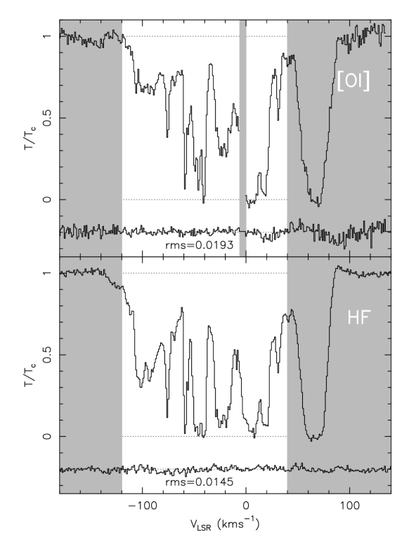
Figure 1: Spectra of [O i] and HF absorption toward Sgr B2(M) divided by the corresponding continua. (Upper) SOFIA/GREAT [O i] spectrum. The lower histogram shows the difference between two independent data subsets divided by 2, which is a measure of the uncertainty in the [O i] spectrum. Gray areas show velocities excluded from the analysis. This includes the Sgr B2 envelope at velocities greater than 40 km s^-1 and the region between -6 and 0 km s^-1, where the [O i] spectrum is contaminated by telluric absorption. (Lower) Average Herschel/HIFI spectrum of HF. The lower histogram shows the difference between the two independent observations divided by 2, which is a measure of the uncertainty in the average spectrum.

We used archival Herschel Heterodyne Instrument for the Far-Infrared (HIFI) (de Graauw et al., 2010) observations of hydrogen fluoride (HF) to determine H₂ column densities in the various velocity components on the line of sight toward Sgr B2. Two independent data sets were used in the analysis, which allows an accurate quantification of the instrumental uncertainties. Both data sets, reduced using the latest HIFI instrument pipeline, were downloaded from the European Space Agency Herschel Science Archive and imported into the Institut de radioastronomie millimétrique (IRAM) Gildas software package for subsequent analysis. The first observation is a Band 5A spectral scan of Sgr B2(M), centered at the same position as the O i spectrum (OBSID 1342204739). The second observation is a 4^′ long north-south strip taken in the double-beam-switch (DBS) observing mode (OBSID 1342205881). The DBS reference beams lie approximately $3^{\prime}$ to the east and west (i.e., perpendicular to the roughly north–south elongation of Sgr B2). Two spectra in the strip closest to Sgr B2(M) ($<10^{\prime\prime}$ offsets) were averaged with uniform weighting to produce the final spectrum used in the analysis. We used spectra taken with the HIFI wide band spectrometer, which provided a spectral resolution of 1.1 MHz over a 4 GHz intermediate frequency (IF) bandwidth. The FWHM HIFI beam size at the HF frequency is $\sim$ 18^′′, about three times larger than the SOFIA beam size at the [O i] frequency. However, the foreground clouds are expected to be extended on such angular scales and to fully cover the background continuum source. This conclusion is supported by the good agreement between the two independent HF spectra taken at positions offset by about half of the HIFI beam.

Figure 1 (lower panel) shows the final HF spectrum, an equally weighted average of the two instrumental polarizations and the two independent observations, resampled to a 1 km s^-1 velocity resolution. The lower histogram shows the difference between the spectral scan and DBS observations divided by 2, which is a measure of the uncertainty in the final HF spectrum. The difference spectrum is very flat and shows no residuals, even at positive velocities, where the background absorption may potentially be contaminated by the Sgr B2 envelope emission (see the HF emission wing at velocities greater than 85 km s^-1). The rms computed in the $-130$ to 40 km s^-1 velocity range is 0.0145, and we used this value as the uncertainty of the HF line-to-continuum ratio in the analysis.

3 Results

To derive the oxygen optical depths and the corresponding column densities in the individual channels, we followed established procedures commonly used in the analysis of HIFI observations of light hydrides (e.g., Neufeld et al. 2010; Lis et al. 2010; Monje et al. 2011). We first derived the optical depth of the [O i] and HF lines ($\tau=-ln[1-T_{L}/T_{C}]$, where $T_{L}/T_{C}$ is the line-to-continuum ratio), assuming that the foreground absorption completely covers the continuum source and that all oxygen atoms are in the ground state. The spiral arm clouds on the line of sight toward Sgr B2 have moderate densities, up to a few times $10^{4}$ cm^-3 (Greaves & Williams, 1994). This is lower than the critical density for the excitation of the 63 $\mu$m O i line ($5.0\times 10^{5}$ cm^-3 for collisions with H₂ and $7.8\times 10^{5}$ cm^-3 for collisions with H; Lique et al. 2018; Goldsmith 2019); the assumption that the entire population is in the ground state is thus well justified. Figure 5 shows the [O i] optical depths and the corresponding column density as a function of velocity.

To determine the oxygen abundance, H₂ and H column densities in the line-of-sight clouds are required. Because of its unique thermochemistry, HF has been shown to be an excellent tracer of H₂ (e.g., Phillips et al. 2010; Neufeld et al. 2010; Sonnentrucker et al. 2010; Monje et al. 2011). The HF abundance with respect to H₂ in diffuse or translucent clouds, determined from a comparison with CH observations, is in the range $(1.1-1.6)\times 10^{-8}$, with an average of $(1.4\pm 0.17)\times 10^{-8}$ (multiple velocity components toward W51, W49N, and NGC6334I; Sonnentrucker et al. 2010; Emprechtinger et al. 2012). We used this value to convert the HF column density to the H₂ column density (Fig. 6). To characterize the atomic gas component on the line of sight toward Sgr B2, we used the H i column densities of Winkel et al. (2017). Figure 7 shows the total hydrogen nucleus column density as a function of velocity, along with the molecular and atomic contributions.

Figure 2 shows the gas-phase atomic oxygen abundance as a function of velocity, derived from the observations of the 63 $\mu$m line. The average abundance with respect to hydrogen nuclei, computed over the $-120$ to +40 km s^-1 velocity range, is $(2.51\pm 0.69)\times 10^{-4}$. The $\pm 1\sigma$ dispersion of the individual measurements computed from the ensemble of 120 independent velocity channels is shown. Black error bars are the formal $1\sigma$ uncertainties of the individual measurements, computed by combining in quadrature corresponding uncertainties in the column densities of the atomic oxygen, atomic, and molecular hydrogen. They are typically smaller than the ensemble dispersion, suggesting the presence of variations in the local atomic oxygen abundance among different velocity components.

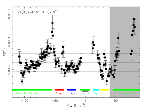
Figure 2: Atomic oxygen abundance relative to hydrogen nuclei as a function of velocity. The mean value of the 120 individual channels within the $-120$ and 40 km s^-1 velocity range is $2.51\times 10^{-4}$, and the dispersion of the individual channels is $0.65\times 10^{-4}$. The horizontal dotted lines mark the mean value and $\pm 1\sigma$ dispersion computed from the ensemble of individual measurements. The black vertical error bars mark $\pm 1\sigma$ uncertainties in the individual channels, as described in the text. Color bars mark velocity ranges corresponding to the 3 kpc, 5 kpc, Sagittarius, and Scutum arms (red, magenta, blue, and yellow, respectively). Velocities corresponding to the Galactic center gas are marked in green and those of the local gas in gray. Channels with saturated absorption are masked. An electronic table with the data used for this figure is available at the CDS.

4 Discussion

The average atomic oxygen abundance toward Sgr B2 derived here, $(2.51\pm 0.69)\times 10^{-4}$ with respect to hydrogen nuclei, is in excellent agreement with the ISO value of $2.7\times 10^{-4}$ (Lis et al., 2001), which was based on ¹³CO column density estimates for the molecular gas component. Figure 3 shows a normalized histogram of the O⁰ abundances in the 120 individual velocity channels. The histogram is non-Gaussian and shows a narrow peak around $2.25\times 10^{-4}$ and a broader shoulder around $3.15\times 10^{-4}$, comparable to the values of $3.1-3.5\times 10^{-4}$ derived by Wiesemeyer et al. (2016) toward W31C, G34.26, and W49N. The origin of the variations in the derived atomic oxygen abundance among different velocity components can be investigated further by using independent observations of additional molecular tracers, including the oxygen ions, CH as a proxy for H₂ (Gerin et al., 2010), argonium as a proxy for purely atomic gas (Schilke et al., 2014), and ammonia as a tracer of high-density gas; such analysis is beyond the scope of the present paper.

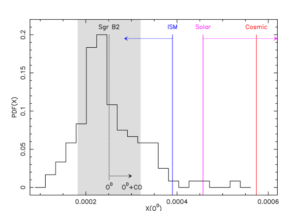
Figure 3: Normalized probability density function (PDF) of the O⁰ abundances in 120 individual velocity channels toward Sgr B2. The vertical dashed black line shows the mean abundance, the gray shaded area $\pm 1\sigma$ departures from the mean, and the black arrow the corresponding approximate gas-phase oxygen content, including atomic oxygen and CO. The vertical red line shows the cosmic standard abundance (Przybilla et al., 2008) and the magenta line the latest solar abundance (Asplund et al., 2005), with the magenta arrow pointing toward the earlier value of Grevesse & Sauval (1998). The blue line is the average UV-derived ISM abundance in the low-density warm gas that is least affected by depletion, with the blue arrow showing the corresponding value for higher mean density site lines (Cartledge et al., 2004).

As a reference, the cosmic standard abundance of oxygen is $(5.75\pm 0.4)\times 10^{-4}$, as measured in a representative sample of unevolved early B-type stars in nearby OB associations (Przybilla et al., 2008). The latest solar photospheric abundance is $4.57\times 10^{-4}$ (Asplund et al., 2005), significantly lower than the earlier Grevesse & Sauval (1998) value of $6.76\times 10^{-4}$. Cartledge et al. (2004) presented a comprehensive analysis of high-resolution Hubble Space Telescope observations of O i and H i Ly $\alpha$ UV absorption along 36 sight lines that probe a variety of Galactic disk environments. They derive an average O/H ratio of $3.90\times 10^{-4}$ in the low-density warm gas that should be least affected by depletion. Sight lines of higher mean density are characterized by a lower average O/H ratio of $2.84\times 10^{-4}$. Taking the higher value as a reference for the atomic oxygen abundance in the ISM gas, our average abundance of $2.51\times 10^{-4}$ on the line of sight toward Sgr B2 corresponds to about 35% gas-phase oxygen depletion. CO will also contribute to the oxygen budget with a typical abundance of $1\times 10^{-4}$ with respect to H₂ in the molecular gas, which is dominant at most velocities on this line of sight (Fig. 7). Adding the two contributions, we derive an estimate of the total gas-phase O⁰ + CO oxygen content toward Sgr B2 of $\sim 3\times 10^{-4}$ with respect to hydrogen nuclei, about 25% lower than the O/H value derived in the low-density warm gas from the UV measurements.

Figure 4 shows the good correlation between the atomic oxygen and total hydrogen nucleus column densities (Pearson’s correlation coefficient 0.85). The average abundance is $2.51\times 10^{-4}$. Error bars mark the formal $1\sigma$ uncertainties of the individual channels. We note that points with the highest O⁰ column densities are located on average above the best-fit line. However, owing to the nonlinear dependence of the opacity on the line-to-continuum ratio at such high column densities, these points have large error bars and the result may not be significant. If we exclude points with the atomic oxygen column densities above $3\times 10^{17}$ cm^-2, the resulting average atomic oxygen abundance is lower by only 2%.

Figure 4: Atomic oxygen column density as a function of total hydrogen nucleus column density. Error bars are $1\sigma$. The dotted line corresponds to a fractional abundance of $2.51\times 10^{-4}$.

5 Conclusions

We have presented an analysis of archival SOFIA/GREAT observations of the [O i] 63 $\mu$m absorption toward the Sagittarius B2(M) continuum source in the Galactic center. The high spectral resolution of the GREAT instrument allows, for the first time, the [O i] absorption from individual line-of-sight clouds to be separated, velocity intervals affected by saturated absorption and telluric absorption to be masked, and accurate atomic oxygen column densities and abundances to be derived. The atomic oxygen column density in the foreground spiral arm clouds toward Sgr B2 is well correlated with the total hydrogen column density, as determined from HF and H i observations, with an average abundance of $(2.51\pm 0.69)\times 10^{-4}$ with respect to H nuclei in individual 1 km s^-1 velocity channels. This value is in good agreement with the earlier ISO measurements on the same line of sight, and about 35% lower than the average O/H ratio of $3.90\times 10^{-4}$ in low-density warm gas derived from UV measurements (Cartledge et al., 2004). If we add a typical gas-phase CO content at $1\times 10^{-4}$ with respect to H₂ in the molecular gas, which is dominant at most velocities on this line of sight (Fig. 7), the total gas-phase oxygen content (O⁰ + CO) on the line of sight toward Sgr B2 is $\sim 3\times 10^{-4}$, or 300 ppm with respect to H, about 25% lower than the low-density warm ISM oxygen abundance derived from UV measurements (Cartledge et al., 2004). With silicates and oxides contributing another 100 ppm (Whittet, 2010), the remaining oxygen fraction is about 175 ppm, which can be viewed as an upper limit for UDO on the line of sight toward Sagittarius B2. However, the expected ice contribution in this density regime is about 125 ppm (Whittet, 2010), leaving little room for UDO.

Appendix A SOFIA data reduction

The data were collected on 2015 July 19, on the southern hemisphere deployment of SOFIA’s Cycle 1, at 11.3 to 11.5 km altitude, under a precipitable water vapor column of typically 6 $\mu$m at zenith. The high-frequency channel of GREAT was tuned to the [O i] line, alternating between the lower and upper sideband, so as to synthesize a sightline velocity interval from $-200$ to $+135$ km s^-1. In the velocity interval considered here, the median single-sideband system temperatures at zenith were 2100 and 2400 K for lower-sideband and upper-sideband tuning, respectively. Atmospheric and Galactic backgrounds were removed by chopping to a reference position at 160^′′ on both sides of Sgr B2(M), at a position angle of $30^{\circ}$ (east to south), that is to say, perpendicular to the object’s elongation. The FWHM beam size of 6.6^′′ was measured from cross-scans on Mars.

The spectra were calibrated to forward-beam brightness temperatures (with a 97% forward efficiency) against loads at ambient and cold temperatures, and then to main-beam brightness temperatures using a 67% main beam efficiency. The $63\,\mu$m [OI] transition is located in the wing of a broad water vapor absorption feature; the applied transmission correction was derived from modeling the measured atmospheric total power emission received in the signal and image bands. In order to minimize the impact of mixer gain drifts, only the off-target spectra immediately following a calibration load measurement were used (i.e., the correction was determined scan-wise and then scaled to the current elevation of each recorded spectrum).

The continuum emission of Sgr B2(M) was obtained from a dedicated double-sideband calibration. While the signal-to-image band gain ratio may deviate from unity (a standard deviation of 5%), the overall reliability of the calibration scheme can be monitored with two tests: First, the saturation of the [OI] line at the systemic velocity defines the zero level for the single-sideband calibration. Second, the mesospheric [OI] line serves as a “beacon” that undergoes the same attenuation in the stratosphere as the astronomical signal. With these precautions, the calibrations and, consequently, the continuum levels of the lower- and upper-sideband tunings were brought into agreement. The spectra, $\mathbf{s}$, of Sgr B2(M) in the lower- and upper-sideband tuning are thus identical within the radiometric noise. The difference between the actually measured spectra ($\mathbf{y_{\mathrm{L}}}$ and $\mathbf{y_{\mathrm{U}}}$ for lower- and upper-sideband tuning, respectively) displays a well-defined linear baseline below $15\,\mathrm{km\leavevmode\nobreak\ s}^{-1}$. Instabilities that arise at velocities above this baseline are from the upper-sideband tuning and can be ignored there thanks to the redundancy with the lower-sideband tuning. The spectra from the two tunings can then be expressed as $\mathbf{y}_{\mathrm{L}}=\mathbf{s}+a_{\mathrm{L}}\mathbf{\nu},\,\,\mathbf{y}_{\mathrm{U}}=\mathbf{s}+a_{\mathrm{U}}\mathbf{\nu}\,,$ where $\nu$ is the frequency in the rest frame of Sgr B2(M). Thanks to the linear baseline fit to the difference spectrum, only two parameters (offset and slope) remained to be optimized, which was done in a way that ensures equal continuum levels on both sides of the line-free portion of the spectra and reproduces the saturated absorption at systemic velocity. The good agreement between the two tunings in the overlapping velocity interval, from $-110$ to $+15\,\mathrm{km\leavevmode\nobreak\ s^{-1}}$, is taken as an assessment of the data processing algorithm.

Appendix B Atomic oxygen and HF column densities

We converted the [O i] optical depth to the atomic oxygen column density assuming that the absorbing gas covers the background continuum source and the entire population is in the lower state (e.g., Neufeld et al. 2010):

$$\int\tau{\rm d}v={{A_{\rm ul}g_{\rm u}\lambda^{3}}\over{8\pi g_{\rm l}}}\,N({\rm O^{0}})=5.365\times 10^{-18}N({\rm O^{0}})\,\,{\rm cm^{2}\,km\,s^{-1}},$$ (1)

where $A_{\rm ul}=8.91^{-5}\,{\rm s}^{-1}$ is the spontaneous radiative decay rate, $g_{\rm u}=3$ and $g_{\rm l}=5$ are the degeneracies of the upper and lower levels, and $\lambda=63.184$ $\mu$m is the transition wavelength. Figure 5 shows the [O i] optical depth (left vertical scale) and the resulting atomic oxygen column density (right vertical scale) in 1 km s^-1 velocity channels as a function of LSR velocity.

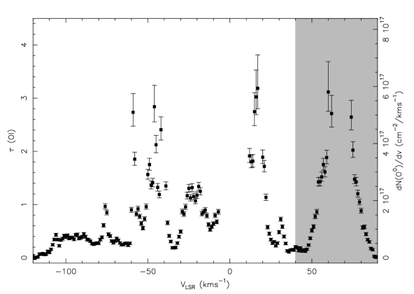
Figure 5: [O i] optical depth (left axis) and atomic oxygen column density (right axis) in 1 km s^-1 channels as a function of velocity. Error bars are $1\sigma$.

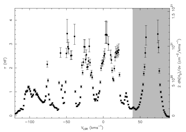
Figure 6: HF optical depth (left axis) and the H nucleus column density in the molecular component (right axis) in 1 km s^-1 channels as a function of velocity. Error bars are $1\sigma$.

The corresponding formula for HF is

$$\int\tau{\rm d}v={{A_{\rm ul}g_{\rm u}\lambda^{3}}\over{8\pi g_{\rm l}}}\,N({\rm HF})=4.157\times 10^{-13}N({\rm HF})\,\,{\rm cm^{2}\,km\,s^{-1}},$$ (2)

with $A_{\rm ul}=2.42^{-2}\,{\rm s}^{-1}$, $g_{\rm u}=3$, $g_{\rm l}=1$, and $\lambda=243.2444$ $\mu$m. Figure 6 shows the HF optical depth and the resulting column density in 1 km s^-1 velocity channels as a function of LSR velocity. Figure 7 shows the total hydrogen nucleus column density as a function of velocity, along with the molecular and atomic contributions, as described in the text.

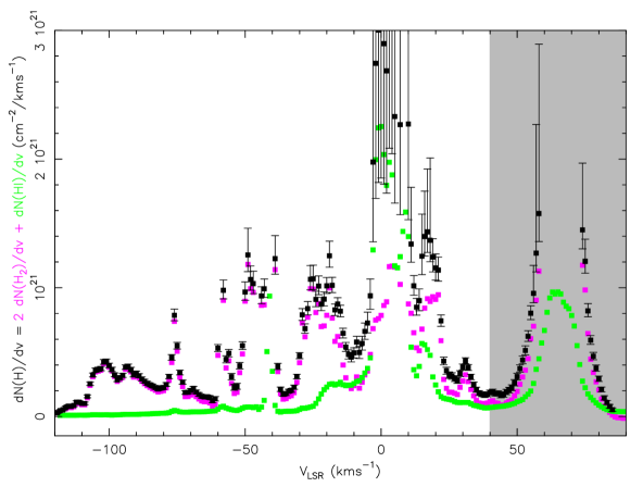
Figure 7: Total hydrogen nucleus column density toward Sgr B2(M) as a function of velocity (black squares). The molecular, $\rm 2\times N(H_{2})$, and atomic, N(H i), components are shown in cyan and green, respectively. Error bars are $\pm 1\sigma$. An electronic table with the data used for this figure is available at the CDS.