Weyl conjecture and thermal radiation of finite systems

Abstract

In this work, corrections for the Weyl law and Weyl conjecture in $d$ dimensions are obtained and effects related to the polarization and area term are analyzed. The derived formalism is applied on the quasithermodynamics of the electromagnetic field in a finite $d$-dimensional box within a semi-classical treatment. In this context, corrections to the Stefan-Boltzmann law are obtained. Special attention is given to the two-dimensional scenario, since it can be used in the characterization of experimental setups. Another application concerns acoustic perturbations in a quasithermodynamic generalization of Debye model for a finite solid in $d$ dimensions. Extensions and corrections for known results and usual formulas, such as the Debye frequency and Dulong-Petit law, are calculated.

Keywords: Weyl law, Weyl conjecture, quasithermodynamics of the electromagnetic field, quasithermodynamics of acoustic perturbations, generalized Debye model

I Introduction

The analysis of thermal radiation is widespread in a large variety of finite-temperature systems. Theoretical research includes treatments based on fluid dynamics and/or quantum field theory. Laboratory and observational applications involve particle phenomenology in colliders, properties of solids in laboratories, characteristics of the cosmic microwave background in dedicated observatories, among many more setups. From lower-dimensional settings to models with arbitrary number of dimensions, thermal radiation frequently plays a significant role.

A common procedure for the investigation of thermal phenomena is based on the definition of a suitable thermodynamic limit within a statistical mechanics model. Usually, the transition from statistical mechanics to thermodynamics implies that the boundary conditions are neglected. In this way, the dependence of the obtained results with the actual volume and shape of the physical system is not considered. Although this approach is useful for many purposes, the strict thermodynamic limit disregards many interesting insights about the actual system of interest. One way to mitigate this problem is to define an intermediary regime between the pure statistical-mechanic treatment and the strict thermodynamic regime, where the volume of the system is large, but finite. This is the so-called quasithermodynamic limit Maslov1 .

On a very general level, the characteristics of thermal radiation in a given setup are directly linked to the asymptotic distribution of eigenvalues of a suitable wave equation. One of the first investigators to explore this connection was Rayleigh, studying the problem of stationary acoustic waves in a cubic room Ray ; Ray2 . Rayleigh’s analysis showed the importance of a term proportional to the volume of the room and to the cube of the mode frequency (the $V\cdot\nu^{3}$ term). This result appeared in the (incorrect) description of the thermal radiation with the Rayleigh-Jeans law. Eventually Planck improved this purely classical analysis, but even within the quantum description the eigenvalue distribution remains unaltered. The same problem, and hence with the same $V\cdot\nu^{3}$ term as the result, emerges in the investigation of the vibration modes in a solid, with the so-called Debye model. In this treatment, Debye proposed that the asymptotic behavior of the eigenvalues do not depend on the shape of the solid. This proposal was rigorously proved by Weyl, and today it is known as the Weyl law. An overview of this development can be seen in Arendt ; Ivrii2 .

A central question considering the strict thermodynamic regime is when the approximation of infinite volume adequately describes a real physical system. For the treatment of this issue, it is necessary an estimate of the terms that are being dropped in the thermodynamic limit. A first step in this direction is given by Weyl conjecture, which predicts corrections proportional to the area of the body. This conjecture has been proven in a variety of domains and in this process, several methods can be applied. For instance, asymptotically expanding the solutions of the Helmholtz equation, using the Neumann-Poincaré construction for the Brownell Green’s function and considering the decomposition of the mode density via multiple reflection expansion Balian ; BalBloc1 .

For many important problems, involving for example the electromagnetic field, vector solutions and polarization effects must be considered. For this purpose, a possible approach is to decompose the vector fields into solutions of the suitable scalar wave equation BalBloc2 ; Balian ; Baltes Baltes ; Liu . Following this program, many works in the pertinent literature indicate that the area term (i.e., the term of Weyl conjecture) does not participate in describing the behavior of the thermal electromagnetic radiation.

Previous comments refer mainly to usual scenarios with three dimensions. But the relevance of the proposed treatment appears in models with different dimensionalities. For instance, the thermodynamic and quasithermodynamic analyses of two-dimensional systems have practical applications in the so-called single-layer materials A15 , with highlights to the graphene B1 . As a more theoretical application, we can mention the thermodynamic properties of photon spheres photon-spheres , thermal radiation of the two-dimensional bosonic and fermionic modes of black holes Geoffrey , as well the description of thermodynamics properties of BTZ black holes btz bh . Considering three-dimensional systems, corrections in thermal radiation play an important role in the analysis of the background microwave radiation Garcia-Garcia . The development is also relevant in the thermodynamic description of the phenomenon of sonoluminescence (hot spot theory), in which pulses of light are created by means of the insertion of sound waves into liquids or gases lumin2 . Systems with more than three spatial dimensions are also explored. For instance, Hawking emission of a black hole is altered in brane-world scenarios Cardoso:2005mh ; Abdalla:2006qj ; rge:2014kra . Thermal radiation phenomena associated with gravitational emission in brane-world models could be significant in the early Universe. Similar effects could be expected in colliders and near active astrophysical objects, within models involving extra dimensions (see for example Maartens:2010ar and references therein). Proposals linking anti-de Sitter geometries and conformal field theories (AdS/CFT correspondences) offer a great variety of applications for $d$-dimensional thermodynamic results Baldiotti:2016lcf ; Baldiotti:2017ywq ; Elias:2018yct ; Fontana:2018drk .

In the present work, Weyl law and its extensions are explored through an intuitive approach. Quasithermodynamic analysis and its description of systems with a finite volume and relevant boundary conditions are a central issue in this article. The developed formalism is applied on the quasithermodynamics of the electromagnetic field in a cavity and acoustic perturbations in a solid. Generalizations for $d$-dimensional setups are derived. One of the contributions of this work is to incorporate polarization effects directly into the asymptotic expansions of the mode distributions, using mixed boundary conditions. We emphasize the role of the area term, showing that, under certain conditions, a distinct quasithermodynamic behavior emerges.

In addition to the correction coming from the eigenvalue distribution, an expected characteristic of the phenomenology of black-body radiation in finite cavities is the existence of a minimum energy. For the two-dimensional case, this issue was studied in stefan 2d . Generalizing this development for arbitrary dimensions, our treatment allows us to compare the effects associated to the minimum energy with those related to corrections of the spectral distribution.

This work is organized as follows. In section II, the proposed formalism associated to the Weyl law is established. In section III, with the techniques introduced, higher-order corrections to the Weyl law are obtained. More complex setups are considered in section IV, where mixed boundary conditions and degeneracies are treated. In section V we turn to physics applications, linking the results previously obtained with thermodynamics and quasithermodynamics. In section VI, the thermodynamic treatment of the electromagnetic field in a finite cavity is conducted. The quasithermodynamics of acoustic perturbations is considered in section VII, where Debye model is analyzed and extended. In section VIII final comments and future perspectives are presented. Further details on the calculation of the hypervolume associated to the axes and counting functions are discussed in appendices A and B.

II Scalar field and Weyl law

Electromagnetic and mechanic perturbations in cavities and solids are the main interest in the present work. However, as we will see later on, the thermodynamics of those systems can be described in terms of a simpler scalar perturbation. Let us consider a scalar field $\psi\left(x_{1},\ldots,x_{d}\right)$ in $d$ dimensions, confined in a cubic cavity of size $L$, which respects the Helmholtz equation,

$$\nabla_{d}^{2}\psi\left(x_{1},\ldots,x_{d}\right)+k^{2}\psi\left(x_{1},\ldots,x_{d}\right)=0\,,\ x_{i}\in\Omega_{d}\,,\ k\in\mathbf{\mathbb{R}}\,.$$ (1)

In Eq. (1), $\nabla_{d}^{2}$ denotes the $d$-dimensional Laplacian. The hypervolumes of domain $\Omega_{d}$ and its boundary $\partial\Omega_{d}$ are given respectively by

$$\left|\Omega_{d}\right|=L^{d}\,,\,\,\,\left|\partial\Omega_{d}\right|=2dL^{d-1}\,.$$ (2)

Two different boundary conditions for Eq. (1) will be initially explored, namely the Neumann condition ($\partial_{n}\psi=0$ at $\partial\Omega_{d}$) and the Dirichlet condition ($\psi=0$ at $\partial\Omega_{d}$).

Solutions of the $d$-dimensional Helmholtz equation (1) can be constructed using the one-dimensional version of (1), which are

$$\phi_{n}^{\pm}\left(x\right)=\frac{e^{-i\pi/4}\pm e^{i\pi/4}}{\sqrt{4L}}\left(e^{ik_{n}x}\pm e^{-ik_{n}x}\right)\,,\ k_{n}=\frac{\pi}{L}n\,,\,\,n=\left\{\begin{array}[c]{c}0,1,2,\ldots\left(+\right)\\ 1,2,3,\ldots\left(-\right)\end{array}\right.\,.$$ (3)

The label ($+$) indicates solutions satisfying Neumann conditions, while ($-$) denotes solutions obeying Dirichlet conditions. From the one-dimensional solutions, $d$-dimensional generalizations can be constructed as

$$\psi^{\pm}\left(x_{1},\ldots,x_{d}\right)=\phi_{n_{1}}^{\pm}(x_{1})\phi_{n_{2}}^{\pm}(x_{2})\cdots\phi_{n_{d}}^{\pm}(x_{d})\,,$$ (4)

with

$$k^{2}=\frac{\pi^{2}}{L^{2}}(n_{1}^{2}+\cdots+n_{d}^{2})\leavevmode\nobreak\ .$$ (5)

It should be noted that, for the Dirichlet case, the solutions with $n_{i}=0$ should be excluded in order to avoid the null solution.

Considering Eq. (5), the set of solutions of the Helmholtz equation (1) can be labeled by points in a discrete lattice. Specifically, we consider the $d$-dimensional Cartesian lattice $L_{\epsilon}^{d}$,

$$L_{\epsilon}^{d}\equiv\left\{(\epsilon_{1},\epsilon_{2},\ldots,\epsilon_{d})\in\mathbb{R}^{d}:\epsilon_{i}=\epsilon n_{i}\,,\ n_{i}=0,1,2,\ldots\right\}\,,$$ (6)

where the (real and positive) $\epsilon$ is the lattice parameter. We denote the region $\tilde{\Omega}_{d}\subset\mathbb{R}^{d}$ as one of the $2^{d}$ sections of the $d$-dimensional sphere of radius $k$, i.e.,

$$\tilde{\Omega}_{d}\equiv\left\{(\epsilon_{1},\epsilon_{2},\ldots,\epsilon_{d})\in\mathbb{R}^{d}:\epsilon_{1}^{2}+\epsilon_{2}^{2}+\cdots+\epsilon_{d}^{2}<k^{2}\,,\ \epsilon_{i}\geqslant 0\right\}\,.$$ (7)

The main questions addressed in the present work can be formulated as counting problems. In this direction, let us define a counting function $N^{(d)}(k)$ as

$$N^{\left(d\right)}\left(k\right)=\left\{\#\left(n_{1},\ldots,n_{d}\right):\frac{\pi^{2}}{L^{2}}\left(n_{1}^{2}+\cdots+n_{d}^{2}\right)<k^{2}\right\}\,.$$ (8)

The function $N^{(d)}(k)$ can be expressed as

$$N^{\left(d\right)}(k)=\mathrm{card}\left(L_{\epsilon}^{d}\cap\tilde{\Omega}_{d}\right)\,,\,\,\epsilon=\frac{\pi}{L}\,,$$ (9)

where “$\mathrm{card}$” denotes the cardinality of the set Suppes . It should be noted that the complete dependence of $N^{\left(d\right)}(k)$ on $k$ is described by $\tilde{\Omega}_{d}$, since the lattice is (for now) fixed. We are interested in the asymptotic behavior of $N^{(d)}(k)$ as $k\rightarrow\infty$.

One method for the analysis is to adopt a “coarse grained” version of the lattice, where the counting of the discrete points is substituted by the calculation of volumes. More specifically, the function $N^{(d)}(k)$ is approximated by the volume $V_{d}(k)$ generated by hypercubes of side length $\epsilon$, centered on the points of the lattice belonging to $L_{\epsilon}^{d}\cap\tilde{\Omega}_{d}(k)$. We illustrate this coarse graining in Figs. 1 and 2 of the next section. The volume of each hypercube is $\epsilon^{d}$, and hence $V_{d}\left(k\right)=\epsilon^{d}N^{(d)}(k)$. The total volume $V_{d}\left(k\right)$ tends to infinity as $k\rightarrow\infty$, $N^{(d)}(k)\rightarrow\infty$ and $\epsilon$ is kept fixed.

Expression (9) and the coarse graining introduced are a well-known algorithm for the counting process, in which the lattice is kept fixed. In the present work, we propose an alternative approach. Instead of fixing $\epsilon$ (that is, the lattice), we fix the volume $V_{d}\left(k\right)$. In other words, we propose to maintain the domain fixed and adjust the lattice. This can be accomplished rescaling $\epsilon_{i}$,

$$\epsilon_{i}\longrightarrow\epsilon_{i}=k^{-1}\epsilon_{i}=\epsilon n_{i}\,,\,\,\epsilon=\frac{\pi}{kL}\,.$$ (10)

With the rescaling, both the counting function $N^{\left(d\right)}\left(k\right)$ and the volume $V_{d}$ become dependent only on the lattice, that is,

$$V_{d}\left(\epsilon\right)=\epsilon^{d}N^{(d)}(\epsilon)\,.$$ (11)

Intuitively, $V_{d}(\epsilon)$ should tend to the volume $|\tilde{\Omega}_{d}|$ as the lattice becomes more dense ($\epsilon\rightarrow 0^{+}$), where

$$\left|\tilde{\Omega}_{d}\right|=2^{-d}\omega_{d}\,,\ \omega_{d}=\frac{\pi^{d/2}}{\Gamma\left(\frac{d}{2}+1\right)}\,,$$ (12)

and $\Gamma$ denotes the usual gamma function. The precise development of this relation will lead to the so-called Weyl law, which will be explicitly shown with the approach proposed in this work.

To clarify the notation, let us denote the counting function for the Neumann case as $N_{+}^{(d)}$, and analogously $N_{-}^{(d)}$ for the Dirichlet case. We focus on the difference in the counting problem considering the Neumann and Dirichlet setup. This difference is a result of the inclusion of the points belonging to the $\epsilon_{i}$-axis for the calculation of $N_{+}^{(d)}$, and the exclusion for $N_{-}^{(d)}$.

Let us treat the Neumann boundary condition first, since (as will be shown in later sections) $N_{-}^{(d)}$ can be expressed in terms of $N_{+}^{(d)}$. The counting function $N_{+}^{(d)}$ can be written as

$$N_{+}^{(d)}(\epsilon)=\sum_{n_{1}=0}^{M(\epsilon)}\cdots\sum_{n_{d-1}=0}^{M(\epsilon)}\left\lfloor\frac{\sqrt{1-\epsilon^{2}(n_{1}^{2}+\cdots+n_{d-1}^{2})}}{\epsilon}\right\rfloor\,,\ M(\epsilon)=\left\lfloor\frac{1}{\epsilon}\right\rfloor\,,$$ (13)

with $\lfloor x\rfloor$ representing the integer function (or floor function) of $x$ Graham . Using the sawtooth function $\eta(x)$, $\eta(x)\equiv x-\lfloor x\rfloor$, Eq. (11) is written as

$$V_{d}^{+}(\epsilon)=\epsilon^{d-1}\sum_{n_{1}=0}^{M(\epsilon)}\cdots\sum_{n_{d-1}=0}^{M(\epsilon)}\sqrt{1-\epsilon^{2}(n_{1}^{2}+\cdots+n_{d-1}^{2})}-\epsilon^{d}\sum_{n_{1}=0}^{M(\epsilon)}\cdots\sum_{n_{d-1}=0}^{M(\epsilon)}\eta\left(\frac{1}{\epsilon}\right)\,.$$ (14)

Since $0\leq\eta<1$, the second term of Eq. (14) obeys the following property:

$$0\leq\epsilon^{d}\sum_{n_{1}=0}^{M\left(\epsilon\right)}\cdots\sum_{n_{d-1}=0}^{M\left(\epsilon\right)}\eta<\epsilon\left[\epsilon+\epsilon M\left(\epsilon\right)\right]^{d-1}\,,$$ (15)

implying that

$$\lim_{\epsilon\rightarrow 0^{+}}{\epsilon^{d}\sum_{n_{1}=0}^{M\left(\epsilon\right)}\cdots\sum_{n_{d-1}=0}^{M\left(\epsilon\right)}\eta}\left(\frac{1}{\epsilon}\right)=0\,.$$ (16)

Previous results lead to the Weyl law, as we will show in the following. Considering the first term in Eq. (14), we observe that

$$\epsilon=\frac{M^{-1}}{1+\eta M^{-1}}\Rightarrow\lim_{\epsilon\rightarrow 0^{+}}{\epsilon}=\lim_{M\rightarrow\infty}\frac{M^{-1}}{1+\eta M^{-1}}=\lim_{M\rightarrow\infty}M^{-1}\,,$$ (17)

and we can write

$$\lim_{\epsilon\rightarrow 0^{+}}{\epsilon^{d-1}\sum_{n_{1}=0}^{M\left(\epsilon\right)}\cdots\sum_{n_{d-1}=0}^{M\left(\epsilon\right)}\sqrt{1-\epsilon^{2}\left(n_{1}^{2}+\cdots+n_{d-1}^{2}\right)}}$$

$$=\lim_{M\rightarrow\infty}{\ \frac{1}{M^{d-1}}\,\sum_{n_{1}=0}^{M\left(\epsilon\right)}\cdots\sum_{n_{d-1}=0}^{M\left(\epsilon\right)}\sqrt{1-\frac{n_{1}^{2}+\cdots+n_{d-1}^{2}}{M^{2}}}}\,.$$ (18)

The last terms in Eq. (18) is the Riemann sum which gives the volume of $\tilde{\Omega}_{d}$. Hence, using Eq. (16), we conclude that

$$\lim_{\epsilon\rightarrow 0^{+}}{V_{d}^{+}}\left({\epsilon}\right)=2^{-d}\omega_{d}\,.$$ (19)

Result (19) is the Weyl law for the scalar field in a cubic cavity, with Neumann boundary conditions.

Although the Weyl law is a well-known result, the procedure adopted here (that is, a coarse graining with a scaling which fixes the domain and modifies the lattice) can be employed in the improvement of the result (19). Also, this approach will allow us to consider different boundary conditions and polarization effects.

III Beyond the Weyl conjecture

Weyl law can be considered as the zero-order correction of the counting function. The first-order correction was conjectured by Weyl and later proven by Ivrii Ivrii1 . In our notation, the Weyl conjecture can be written as

$$\epsilon^{d}N_{\pm}^{(d)}(\epsilon)=2^{-d}\omega_{d}\pm 2^{-d}d\omega_{d-1}\epsilon+O(\epsilon^{w_{d}})\,,$$ (20)

where $w_{d}=\left(d^{2}-d+1+1/d\right)/\left(d-1\right)$ Brownell . In the “big-$O$” sense, no higher-order corrections are known Ivrii1 ; Brownell . Although for the scalar case the above correction is always the most relevant, as we will see, when considering the vector problem this correction may cancels. Therefore, its important to go beyond the first correction. For this goal a special type of “averaged corrections” can be considered. It is defined using Gaussian logarithmic averages, or the called Brownell’s $\tilde{O}$ formalism Brownell . One says that $f=\tilde{O}\left(g\right)$ if, for some $x_{0}$,

$$\left|\int_{x_{0}}^{\infty}e^{-\frac{1}{2}\rho^{2}\left(\ln\frac{y}{x^{\prime}}\right)^{2}}\leavevmode\nobreak\ \left.\frac{df(x)}{dx}\right|_{x^{\prime}}\leavevmode\nobreak\ dx^{\prime}\right|\leq\delta_{\rho}g\left(y\right)\,,$$ (21)

for every $\rho>0$ and some $\delta_{\rho}<\infty$. For the case $d=2,3$, it is found that

$$\epsilon^{2}N_{\pm}^{(2)}(\epsilon) =\frac{\pi}{4}\pm\epsilon+\frac{\epsilon^{2}}{4}+\tilde{O}(\epsilon^{\tilde{w}_{2}})\,,$$ (22)

$$\epsilon^{3}N_{\pm}^{(3)}(\epsilon) =\frac{\pi}{6}\pm\frac{3\pi}{8}\epsilon+\frac{3}{4}\epsilon^{2}\pm\frac{\epsilon^{3}}{8}+\tilde{O}(\epsilon^{\tilde{w}_{3}})\,,$$ (23)

where $\tilde{w}_{2}>2$ and $\tilde{w}_{3}>3$ Baltes e Kn ; Brownell . As will be seen below, the corrections (22)-(23) are given by a polynomial expansion whose coefficients are related to the geometric “shape” of the $\tilde{\Omega}_{d}$ boundary. Based on this geometric argument, it will be seen that we can always decompose $\epsilon^{d}N_{+}^{(d)}(\epsilon)$ as the sum of two contributions: one continuous component, that we will denote by $\mathcal{F}^{(d)}(\epsilon)$, and other non-continuous.

Our goal in this section is to explore the relation between the functional form of $\mathcal{F}^{(d)}(\epsilon)$ and the corrections derived from the Brownell formalism. We will employ a “bottom-up approach”, considering in detail particular values for $d$, and then extrapolating the results for general $d$.

The one-dimensional case ($d=1$) is trivial, however it is crucial to construct the bottom-up approach. For this case, the Brownell corrections coincide with the exact corrections. From Eq. (13), the counting function for Neumann boundary condition is given by

$$\epsilon N_{+}^{\left(1\right)}\left(\epsilon\right)=1-\epsilon\eta\left(\epsilon^{-1}\right)\sim 1\Rightarrow\mathcal{F}^{(1)}(\epsilon)=1\,.$$ (24)

For the Dirichlet boundary condition the result is similar:

$$\epsilon N_{-}^{\left(1\right)}\left(\epsilon\right)=\epsilon[N_{+}^{\left(1\right)}\left(\epsilon\right)-1]=1-\epsilon[1+\eta\left(\epsilon^{-1}\right)]\sim 1\,.$$ (25)

For the two-dimensional Neumann scenario, given the shape of $\tilde{\Omega}_{2}$ boundary, we can decompose $\epsilon^{2}N_{+}^{(2)}$ as

$$\epsilon^{2}N_{+}^{(2)}(\epsilon)=\frac{\pi}{4}+\text{axes-boundary area}+\text{area of the boundary curve}\,.$$ (26)

This result is illustrated in Fig. 1. More precisely, the “axes-boundary area” is the excess area localized around the axes (which are not included in $\tilde{\Omega}_{2}$). As seen in Fig. 1, this quantity is

$$\text{axes-boundary area}=\epsilon+\frac{\epsilon^{2}}{4}\,.$$ (27)

Notice that we are considering the contribution of each axis in the interval $\left[0,1\right]$, implying that the contribution of the central square is $\epsilon{}^{2}/4$. The contribution of the area of the boundary curve is unknown. However we know that it is described by a non-continuous function, otherwise $N_{+}^{(2)}(\epsilon)$ would be a continuous function and we know that this is not true. Hence, it follows that $\mathcal{F}^{(2)}(\epsilon)$ in this case is

$$\mathcal{F}^{(2)}(\epsilon)=\frac{\pi}{4}+\epsilon+\frac{\epsilon^{2}}{4}\,,$$ (28)

which agrees with the Brownell corrections given in Eq. (22) for the Neumann case.

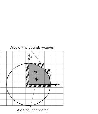
Figure 1: Two-dimensional coarse graining and lattice considered in the counting process. The solid gray region contributes with an area equals to $\pi/4$ (one fourth of the circle) and each axis contributes with an area equals to $\epsilon/2$.

For the two-dimensional Dirichlet scenario, note that we can relate $N_{-}^{(2)}$ and $N_{+}^{(2)}$ as

$$N_{+}^{(2)}(\epsilon)=\underset{\text{points outside the axes}}{\underbrace{N_{-}^{(2)}(\epsilon)}}+\underset{\text{points at the axes}}{\underbrace{2N_{-}^{(1)}(\epsilon)+1}}\,.$$ (29)

Isolating $N_{-}^{(2)}$ and using results (24) and (28), we obtain the Brownell corrections given in Eq. (22) for Dirichlet.

The analysis for the three-dimensional case can be conducted in an analogous manner. To illustrate the development, let us consider Fig. 2, the generalization of two-dimensional lattice diagram (one eighth of the three-dimensional sphere instead of one fourth of the two-dimensional circle).

With the three-dimensional lattice with Neumann boundary conditions, we get that $\mathcal{F}^{(3)}(\epsilon)$ for this case is

$$\mathcal{F}^{(3)}(\epsilon)=\frac{\pi}{6}+\frac{3\pi}{8}\epsilon+\frac{3}{4}\epsilon^{2}+\frac{\epsilon^{3}}{8}\,.$$ (30)

Again, the Brownell corrections for Neumann given in Eq. (23), are obtained.

For the three-dimensional case with Dirichlet boundary conditions, the counting function can be decomposed as

$$N_{+}^{\left(3\right)}\left(\epsilon\right)=\underset{\text{points outside the axes}}{\underbrace{N_{-}^{\left(3\right)}\left(\epsilon\right)}}+\underset{\text{points at the faces}}{\underbrace{3N_{-}^{\left(2\right)}\left(\epsilon\right)}}+\underset{\text{points at the axes}}{\underbrace{3N_{-}^{\left(1\right)}\left(\epsilon\right)+1}}\,.$$ (31)

Using previous results, we obtain expression (23).

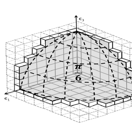
Figure 2: Three-dimensional coarse graining and axes-boundary area. The dotted dark lines represent the $1/8$ of the sphere, that contributes with $\pi/6$. The solids part of the cubes represents the axes-boundary area. The center cube contributes with $\epsilon^{3}/8$. The cubes in each axis contributes with $\epsilon^{2}/4\,$. The cubes in the faces represents $3$ times $1/4$ of the area of the circles, i.e., $3\pi/4$ times $\epsilon$. But only half this value, i.e., $3\pi\epsilon/8$, contributes.

After studying the cases $d=2$ and $d=3$ in detail, we can generalize these results to higher dimensions. Let us initially consider the $d$-dimensional scenario with Neumann boundary conditions. As in Eq. (26), the counting function $\epsilon^{d}N_{+}^{(d)}$ can be expressed as the sum of three contributions: the term $|\tilde{\Omega}_{d}|$, the hypervolume associated to the axes and the hypervolume of the boundary hypersurface. In appendix A, we show that the hypervolume associated to the axes is given by

$$\text{Hypervolume of the axes}=\sum_{n=1}^{d}{\binom{d}{n}2^{-d}\omega_{d-n}\epsilon^{n}}\,,$$ (32)

where

$${\binom{d}{n}=\frac{d!}{n!\left(d-n\right)!}\leavevmode\nobreak\ .}$$ (33)

Hence,

$$\mathcal{F}^{\left(d\right)}\left(\epsilon\right)=\sum_{n=0}^{d}{\binom{d}{n}2^{-d}\omega_{d-n}\epsilon^{n}\leavevmode\nobreak\ }\,.$$ (34)

The result obtained above generalizes the corrections (22)-(23) to an arbitrary dimension. By repeating the procedure realized in Brownell for $d=2,3$, and the using the Theorem (8.17) on this reference, we can find

$$\epsilon^{d}N_{+}^{(d)}(\epsilon)=\mathcal{F}^{(d)}\left(\epsilon\right)+\tilde{O}(\epsilon^{\tilde{w}_{d}})\,,\tilde{w}_{d}>d\,.$$ (35)

The Dirichlet case can be obtained using a generalization of expressions (29) and (31). This generalization is constructed in Appendix B, and the final expression can be condensed into

$$\epsilon^{d}N_{\pm}^{\left(d\right)}\left(\epsilon\right)=\sum_{n=0}^{d}\left[\left(-1\right)^{\frac{d-n}{2}}\right]^{1\mp 1}{\binom{d}{n}2^{-d}\omega_{d-n}\epsilon^{n}}+\tilde{O}\left(\epsilon^{\tilde{w}_{d}}\right)\,.$$ (36)

Expression (36) is the main result of this section. Note that this equation also maintains the “alternating symmetry” observed for the cases $d=2,3$, when we go from Neumann to Dirichlet. If the coefficients do not follow this binomial pattern, the alternating symmetry in the signs of coefficients is broken.

Rewriting expression (36) in terms of the variable $k$, we have the results provided by Brownell’s formalism for higher orders,

$$N_{\pm}^{\left(d\right)}\left(k\right)=\frac{1}{2^{d}}\sum_{n=0}^{d}\left[\left(-1\right)^{\frac{d-n}{2}}\right]^{1\mp 1}{\binom{d}{n}\frac{\pi^{(n-d)/2}L^{d-n}}{\Gamma\left(\frac{d-n}{2}+1\right)}k^{d-n}}+\tilde{O}\left(k^{d-\tilde{w}_{d}}\right)\,,$$ (37)

where $\tilde{w}_{d}>d$.

IV Mixed boundary conditions and degeneracies

From the results involving Neumann and Dirichlet cases discussed, it is possible to treat more complex boundary conditions, dubbed here as “mixed boundary conditions”. Also, in the present section, we will consider the effects of degeneracies in the spectra. Those setups model physical systems described by Helmholtz equation which will be considered in this work. Further interesting examples (not directly addressed here) can be found in Hacyan ; Actor .

In the present development, mixed boundary conditions are constructed imposing Neumann and Dirichlet conditions in different axes. The solutions of Helmholtz equation (1) under these conditions can be written as

$$\psi_{M}\left(x_{1},\ldots,x_{d}\right)=\phi^{\pm}\left(x_{1}\right)\cdots\phi^{\pm}\left(x_{d}\right)\,.$$ (38)

In $d$ dimensions, the number of possible scenarios with mixed boundary conditions is $2^{d}$, including the ones which are entirely Dirichlet or Neumann. In any case, the counting function (referred generally as $N_{M}^{(d)}$ for an arbitrary boundary condition) can be decomposed as a linear combination in the form

$$N_{M}^{\left(d\right)}(\epsilon)=\sum_{n=0}^{d}A_{n}N_{-}^{\left(n\right)}\left(\epsilon\right)\,,$$ (39)

where the coefficients $\{A_{n}\}$ are related to the boundary conditions and possible degeneracies. For example, result (111) for the Neumann case without degeneracies is recovered with $A_{n}=\binom{d}{n}$ (see Appendix B for details). This expression (111) can be generalized with the consideration of vector fields associated to the Helmholtz equation. This development will be necessary to the treatment of degeneracies. In the vector-field problem, beside the $d$ modes $\{n_{1},n_{2},\ldots,n_{d}\}$, there are also $d$ components for the fields, $\{F_{n_{1}\cdots n_{d}}^{i}\,,\,i=1,\ldots,d\}$. However, contrary to the scalar field, the internal degrees of freedom of the vector fields must be taken into account. There is, the polarization of the vector field is an issue.

Possible polarizations can be transverse and longitudinal. Indeed, the vector fields can be expressed as

$$F_{n_{1}\cdots n_{d}}^{i}=F^{0i}\prod_{k=1}^{\chi}\phi_{n_{k}}^{+}\prod_{j=\chi+1}^{d}\phi_{n_{j}}^{-}\,,\,\,i=1,\ldots,d\,,$$ (40)

with constants $F^{0i}\in\mathbf{\mathbb{C}}$. Following the development which leaded to Eq. (111), non-trivial solutions can be separated into $(\chi+1)$ classes: those in which only one $n_{i}$ is null, those in which two $n_{i}$ are null, and so on, up to those which $\chi$ of the $n_{i}$ are equal to zero. Let us label these classes as “class zero”, “class one”, and so on, respectively.

The solutions where $\chi$ of the possible $n_{k}$ are null (forming the class $\chi$) have only one non-null component $F_{n_{1}\cdots n_{d}}^{i}$. These solutions are polarized in the direction of this component. In the same way, solutions with $(\chi-1)$ of the possible $n_{i}$ being null have two non-null components, and consequently two possible polarizations. Hence, the class $n$ has a degenerescence equal to

$$\xi_{\chi-i}^{\left(d,\chi\right)}=i+1\,,\,\,\,i=0,\ldots,\chi-1\,,\,\,\,\chi\leq d\,.$$ (41)

For the class zero, where none of the $n_{i}$ is null, all the components $F_{n_{1}\cdots n_{d}}^{i}$ can be non-null and we have $d$ degrees of freedom, $\xi_{0}^{\left(d,\chi\right)}=d\,$. This counting of the degrees of freedom considers only the effect of the boundary conditions. In addition, one can also impose the orthogonality condition, which prevents the longitudinal modes. This condition requires that the amplitude vector to be perpendicular to the wave vector,

$$\sum_{n=1}^{d}k_{n}F^{0n}=0\,,$$ (42)

which reduces by one the number of degrees of freedom of the zero class configuration. Therefore, we can write

$$\xi_{0}^{\left(d,\chi\right)}=\xi_{0}^{\left(d\right)}=d-\tilde{\xi}\,,$$ (43)

where $\tilde{\xi}=1$ for systems which admit only transverse perturbations and $\tilde{\xi}=0$ for cases where longitudinal perturbations are considered.

As commented in Appendix B, each class $n$ of the $(\chi+1)$ vector solutions behaves as the Dirichlet problem in $(d-n)$ dimensions. The class with only one of the $n_{i}$ equal to zero (degenerescence equal to $\xi_{1}^{\left(d,\chi\right)}$) can be divided in $d$ sub-classes ($d$ cases where $n_{j}=0$). If two of the solutions have $n_{j}=0$ (degenerescence $\xi_{2}^{\left(d,\chi\right)}$), the subclass can then be further separated in $\binom{d}{2}$ sets. The process continues, until eventually new sub-classes can not be produced. Given the counting process presented, the total number of modes can be expressed as the composition of the classes and sub-classes thus constructed,

$$N_{\chi}^{\left(d\right)}=\sum_{n=0}^{\chi}\left(\#n\text{-class}\right)\times\left(n\text{-degenerescence}\right)\times N_{-}^{\left(d-n\right)}\,,$$ (44)

or

$$N_{\chi}^{\left(d\right)}\left(\epsilon\right)=\sum_{n=0}^{\chi}\binom{d}{n}\xi_{n}^{(d,\chi)}N_{-}^{\left(d-n\right)}\left(\epsilon\right)\,,$$ (45)

with $N_{-}^{\left(m\right)}$ given by Eq. (37), $\xi_{m}^{(d,\chi)}$ in Eq. (41) for $m>0$ and $\xi_{0}^{(d,\chi)}$ in Eq. (43). We emphasize that expression (45) is one of the main results of the present work. For $\chi=d$ and no polarization ($\xi_{i}^{\left(d\right)}=1\,,\ \forall i=0,\ldots,d$), Eq. (111) in Appendix B is recovered.

In the following sections we will apply the formalism developed in concrete scenarios. Namely, we will discuss the thermodynamics of the electromagnetic field in a hypercubic cavity and acoustic perturbations in a generalized version of Debye model.

V Thermodynamic and quasithermodynamic limits

From the Weyl law and its extensions, we turn to physics applications. The goal of this section is to connect the derived expansions for the counting functions with thermodynamic analyses. In this context, corrections of the Weyl law will correspond to the transition from the strict thermodynamic limit to the quasithermodynamic approach.

Let us assume a semi-classical treatment, with the physical system of interest being described by solutions of the Helmholtz equation (1). In the treatment, we consider a $d$-dimensional cubic box with side length $L$ populated by a thermal gas. The gas is composed by effective massless particles (actually modes associated to electromagnetic or acoustic perturbations) with a well-defined energy and subjected to the Bose-Einstein statistics. The system is supposed to be in thermal equilibrium with constant temperature $T$. The number of modes is not conserved, and hence the chemical potential $\mu$ is null. Since the temperature and chemical potential are fixed, the grand canonical ensemble is assumed.

A macroscopic treatment is established if a thermodynamic limit can be achieved. Since that we are employing a grand canonical ensemble, the strict thermodynamic limit is defined as Kuzemsky

$$|\Omega_{d}|\rightarrow\infty\,\,\text{with}\,\,T\,\,\text{fixed}\,\,\text{and}\,\,\mu=0\,\,,$$ (46)

where $|\Omega_{d}|$ is the hypervolume of the domain $\Omega_{d}$. As seen from Eq. (2), this condition implies that

$$LT\rightarrow\infty\,\,\text{with}\,\,T\neq 0\,\,\text{fixed}\,\,\text{and}\,\,\mu=0\,.$$ (47)

It is also important to consider not only the thermodynamic limit, but also how this limit is approached. Hence, we establish the quasithermodynamic limit Maslov1 as

$$|\Omega_{d}|\,\,\text{large but finite, with}\,\,T\,\,\text{fixed}\,\,\text{and}\,\,\mu=0\,\,.$$ (48)

The quasithermodynamic is particularly relevant in the present work, where finite cavities or solids are considered.

Given that the system of interest is compatible with thermodynamic and quasithermodynamic limits, the associated partition function can be written as

$$\ln Z=-\int_{0}^{\infty}\,D(\omega)\,\ln\left[1-\exp\left(-\frac{\hbar\omega}{k_{B}T}\right)\right]\,\mathrm{d}\omega\,,$$ (49)

where $D(\omega)$ is the spectral density function. Expression (49) can be seen as the Thomas-Fermi approximation for the exact grand canonical partition function. From $Z$, all the associated thermodynamic and quasithermodynamic quantities can be readily calculated. For example, the internal energy is given by

$$U=k_{B}T^{2}\frac{\partial}{\partial T}\,\left(\ln Z\right)\,.$$ (50)

In a practical implementation of the quasithermodynamic limit, combined with the assumption that the temperature of the system is fixed, the box length $L$ should be large enough so that Elias:2018yct

$$\frac{k_{B}}{\hbar c}\,LT\gg 1\,,\,\,\text{with $LT$ kept finite.}$$ (51)

As reference, $k_{B}/(\hbar c)\approx 436.7\,\text{K}^{-1}\,\text{m}^{-1}$ in SI units. The relation between the spectral density $D$ in the partition function (49) and the counting functions studied in the previous sections (collectively denoted by $N^{(d)}$) is given by

$$D(\omega)\,\mathrm{d}\omega=\frac{\mathrm{d}N^{(d)}(\omega)}{\mathrm{d}\omega}\,\mathrm{d}\omega\,.$$ (52)

It follows that the Weyl law (19) is connected with the strict thermodynamic limit (47) when only the term with highest power of $LT$ is considered in the asymptotic expansion of the counting function. For the link between extensions of Weyl law and the quasithermodynamic limit (51), subdominant corrections on powers of $LT$ are also considered in this expansion. It should be noted that, although result (45) for the counting function is valid for any values of $L$, it is only when condition (51) is satisfied that the integral form (49) of the partition function can be employed.

VI Quasithermodynamics of the electromagnetic field

A first application of the developed formalism involves quasithermodynamics of the electromagnetic field in a (hyper)cubic cavity. Let us consider a cubical cavity in $d$ dimensions with side length $L$. Its faces are supposed to be perfect conductors, surrounding a vacuum region. The electric field inside the cavity satisfies a wave equation characterized by a velocity equals to $c$. Also, the conductivity of the walls guaranties that the tangential components of the electric field at the walls are null.

The components of the electric field inside the cavity are given by Liverpool

$$E_{n_{1}\cdots n_{d}}^{i}\left(x_{1},\ldots,x_{d}\right)=E^{0i}\times\phi_{n_{1}}^{-}\left(x_{1}\right)\cdots\phi_{n_{i}}^{+}\left(x_{i}\right)\cdots\phi_{n_{d}}^{-}\left(x_{d}\right)\,,$$ (53)

where each component satisfies a mixed boundary condition (40) with $\chi=1$. Furthermore, as only transverse modes are present, we have $\tilde{\xi}=1$ in Eq. (43). Hence, using result (45), we find that the number of independent modes $N_{\text{em}}^{\left(d\right)}=N_{1}^{\left(d\right)}$ is given by

$$N_{\text{em}}^{\left(d\right)}\left(\omega\right)=\frac{1}{2^{d}}\left[\frac{\left(d-1\right)}{c^{d}\pi^{d/2}}\frac{\left(\omega L\right)^{d}}{\Gamma\left(\frac{d}{2}+1\right)}+\frac{d\left(3-d\right)}{c^{d-1}\pi^{\left(d-1\right)/2}}\frac{\left(\omega L\right)^{d-1}}{\Gamma\left(\frac{d-1}{2}+1\right)}\right]\,.$$ (54)

In Eq. (54), it was assumed the vacuum dispersion relation $k=\omega/c$ for the electromagnetic field.

For the three-dimensional case we have the well-known quadratic term cancellation in $\omega$ Baltes Baltes ; Liu . In this case, we consider the next correction term in Eq. (45), furnishing

$$N_{\text{em}}^{\left(3\right)}=\frac{L^{3}}{3\pi^{2}c^{3}}\omega^{3}-\frac{3L}{2\pi c}\omega\,.$$ (55)

Result (55) agrees with Baltes Baltes ; Baltes e Kn ; Baltes S ; Liu . However, Eq. (54) shows that this cancellation of the “area” term for the electromagnetic field only occurs in the three-dimensional case. This implies a drastic difference in $d=3$ scenario when comparing with other dimensionalities.

The spectral density $D_{\text{em}}^{\left(d\right)}$ can be calculated deriving expression (54) with respect to $\omega$,

$$D_{\text{em}}^{\left(d\right)}=\frac{\mathrm{d}N_{\text{em}}^{\left(d\right)}}{\mathrm{d}\omega}=\frac{1}{2^{d}}\left[\frac{d\left(d-1\right)L^{d}\omega^{d-1}}{\pi^{d/2}\Gamma\left(\frac{d}{2}+1\right)c^{d}}+\frac{d\left(d-1\right)\left(3-d\right)L^{d-1}\omega^{d-2}}{\pi^{\left(d-1\right)/2}\Gamma\left(\frac{d-1}{2}+1\right)c^{d-1}}\right]\,.$$ (56)

Hence, the internal energy of the system can be written as

$$U^{\left(d\right)}=\int_{0}^{\infty}D_{\text{em}}^{\left(d\right)}\left(\omega\right)\frac{\hbar\omega}{\exp\left(\frac{\hbar\omega}{k_{B}T}\right)-1}\leavevmode\nobreak\ \mathrm{d}\omega=k_{B}\left[\left(d-1\right)\theta_{d}L^{d}T^{d+1}+\left(3-d\right)\frac{d}{2}\theta_{d-1}L^{d-1}T^{d}\right]\,,$$ (57)

where $\theta_{m}$ is defined as

$$\theta_{m}\equiv\frac{\zeta\left(m+1\right)\Gamma\left(m+1\right)m}{2^{m}\pi^{m/2}\Gamma\left(\frac{m}{2}+1\right)}\frac{k_{B}^{m}}{\hbar^{m}c^{m}}\,.$$ (58)

The term $\zeta\left(z\right)$ in Eq. (58) denotes the Riemann zeta function. Expression (57) can be seen as an improved version of the Stefan-Boltzmann law for the electromagnetic field in a hypercubic cavity, in a quasithermodynamic treatment.

In the strict thermodynamic limit, that is, when the correction is not considered, we recover the Stefan-Boltzmann law in $d$ dimensions. In the strict thermodynamic regime, the (improved) result (57) can be compared with Landsberg ; Alnes . However, in those references the authors impose that $\xi_{\text{em}}^{(d)}=\xi_{0}^{\left(d\right)}=2$ for the polarization of the $d$-dimensional electric field (as done for the three-dimensional scenario). The observation that $\xi_{\text{em}}^{(d)}=d-1$ is the correct factor was made in Comment .

It is important to stress that, while the enforcement that $\xi_{\text{em}}^{(d)}=2$ for any dimension corresponds to a simple factor for the main term of several thermodynamic quantities, this choice has a very drastic effect for the correction terms in the quasithermodynamic analysis. For instance, when considering the quasithermodynamics, the general enforcement of $\xi_{\text{em}}^{(d)}=2$ would imply the cancellation of the first correction for any value of $d$ (not appropriate), and not for $d=3$, as we have obtained.

The quasithermodynamic Stefan-Boltzmann law (57) can also be rewritten as

$$\frac{U^{\left(d\right)}}{L^{d}}=\int_{0}^{\infty}B^{\left(d\right)}\left(\omega,T,L\right)\leavevmode\nobreak\ \mathrm{d}\omega\,,$$ (59)

implying that

$$B^{\left(d\right)}\left(\omega,T,L\right)=\left[\frac{\omega}{\Gamma\left(\frac{d}{2}+1\right)}-\frac{c\left(d-3\right)\sqrt{\pi}}{\Gamma\left(\frac{d-1}{2}+1\right)}\frac{1}{L}\right]\frac{d\left(d-1\right)\hbar\omega^{d-1}}{2^{d}\pi^{d/2}c^{d}\left[\exp\left(\frac{\hbar\omega}{k_{B}T}\right)-1\right]}\,.$$ (60)

Expression (60) is a quasithermodynamic version of the Planck formula. This result describes the effects of the boundedness of the cavity on the spectral density of the electromagnetic field.

For the two-dimensional case, a more detailed discussion is in order. Our results for $d=2$ can be compared with the analysis presented in stefan 2d . An interesting remark suggested in stefan 2d is that size effects prevent arbitrarily low frequencies in the system. With this observation, particularized here for a square system of area $L^{2}$, the authors propose an internal energy $U$ with the form

$$U=2\int_{\omega_{\min}}^{\infty}D\left(\omega\right)\frac{\hbar\omega}{\exp\left(\frac{\hbar\omega}{k_{B}T}\right)-1}\leavevmode\nobreak\ \mathrm{d}\omega\,,\,\,D\left(\omega\right)=\frac{L^{2}\omega}{2\pi c^{2}}\,,\,\,\omega_{\min}=\frac{\sqrt{2}\pi c}{L}\,.$$ (61)

The integral in Eq. (61) can be solved by making the change $x=t+x_{\min}$, where

$$x\equiv\frac{\hbar\omega}{k_{B}T}\,,\,\,x_{\min}\equiv\frac{\hbar\omega_{\min}}{k_{B}T}=\frac{\sqrt{2}\pi\hbar c}{k_{B}TL}\,.$$ (62)

One obtains

$$U\left(x_{\min}\right)=\frac{k_{B}^{3}}{\pi\hbar^{2}c^{2}}\,L^{2}T^{3}S\left(x_{\min}\right)\,,$$ (63)

$$S\left(x_{\min}\right)=2\mathrm{Li}_{3}\left(e^{-x_{\min}}\right)+2x_{\min}\mathrm{Li}_{2}\left(e^{-x_{\min}}\right)+x_{\min}^{2}\mathrm{Li}_{1}\left(e^{-x_{\min}}\right)\,,$$ (64)

where the polylogarithm function $\mathrm{Li}_{s}\left(z\right)$ is defined as

$$\mathrm{Li}_{s+1}\left(z\right)=\frac{1}{\Gamma\left(s+1\right)}\int_{0}^{\infty}\frac{t^{s}}{\exp\left(t\right)/z-1}\leavevmode\nobreak\ \mathrm{d}t\,.$$ (65)

Following the development in stefan 2d , the term $S\left(x_{\min}\right)$ is expanded around $x_{\min}=0$,

$$S(x_{\min})=2\zeta(3)-\frac{x_{\min}^{2}}{2}+\frac{x_{\min}^{3}}{6}-\frac{x_{\min}^{4}}{48}-\frac{x_{\min}^{6}}{4320}+O\left(x_{\min}^{7}\right)\,.$$ (66)

Observe that the expansion close to $x_{\min}=0$ is equivalent to consider $\left[k_{B}/(\hbar c)\right]\,LT\gg 1$, as one sees from the definition of $x_{\min}$ in Eq. (62). Finally, using the expansion (66), and keeping only the first-order term $x_{\min}^{2}$, the approach from stefan 2d furnishes

$$U=\frac{2\zeta\left(3\right)}{\pi}\frac{k_{B}^{3}}{\hbar^{2}c^{2}}L^{2}T^{3}-\pi k_{B}T\,.$$ (67)

We note that the first term in Eq. (67) differs from the result (57) presented in this work by a factor of $2$. This discrepancy is just a consequence of the authors in stefan 2d using the developments of Landsberg which, as previously commented, assume that $\xi_{\text{em}}^{(d)}=2$ for any value of $d$. However, as a more important remark, it is possible to see from Eq. (61) that, while considering the size effects on the minimum frequency, these effects on the density of the modes $D\left(\omega\right)$ are not taken into account. In other words, the integrand of $U$ in Eq. (61) is correct only in the thermodynamic limit.

We propose an improvement of the results in stefan 2d by considering size effects for both the minimal frequency and the density of the modes. Following the procedure that leads to Eq. (64), but using $D_{\text{em}}^{\left(2\right)}$ of Eq. (56) instead of $D(\omega)$ in the integrand of the internal energy $U$ in expression (61), we get

$$U_{\text{em}}^{\left(2\right)}=\pi k_{B}T\left[x_{\min}^{-2}S\left(x_{\min}\right)+\frac{\sqrt{2}}{\pi}x_{\min}^{-1}\tilde{S}\left(x_{\min}\right)\right]\,,$$ (68)

with $S(x_{\min})$ presented in Eq. (64) and

$$\tilde{S}\left(x_{\min}\right)=\mathrm{Li}_{2}\left(e^{-x_{\min}}\right)+x_{\min}\mathrm{Li}_{1}\left(e^{-x_{\min}}\right)\,.$$ (69)

The expansion of $\tilde{S}(x_{\min})$ around $x_{\min}=0$ gives

$$\tilde{S}\left(x_{\min}\right)=\frac{\pi^{2}}{6}-x_{\min}+\frac{x_{\min}^{2}}{4}-\frac{x_{\min}^{3}}{36}+\frac{x_{\min}^{5}}{3600}+O\left(x_{\min}^{6}\right)\,.$$ (70)

Substituting the results (66) and (70) in Eq. (68), and keeping only terms of order up to $x_{\min}^{2}$, we obtain

$$U_{\text{em}}^{\left(2\right)}=\frac{\zeta\left(3\right)}{\pi}\frac{k_{B}^{3}}{\hbar^{2}c^{2}}L^{2}T^{3}+\frac{\pi k_{B}^{2}}{6\hbar c}LT^{2}-\left(\frac{1}{2}+\frac{\sqrt{2}}{\pi}\right)\pi k_{B}T\,.$$ (71)

In addition to the already mentioned factor of $2$, and a correction of $\sqrt{2}/\pi$ in the last term in Eq. (67), we highlight the appearance of an “area” term proportional to $T^{2}$. This new term is the leading correction on the quasithermodynamics limit.

It is important to notice that the second term in Eq. (71), that is, the leading correction, is precisely the last term presented in Eq. (57) for $d=2$. This is a consequence of the fact that $S$ in Eq. (66) does not have a linear term (i.e., a term proportional to $x_{\min}$). The existence of such linear term would change the second term in Eq. (57).

The above procedure for the two-dimensional scenario can be generalized to arbitrary dimensions. In this case, to consider a minimal energy implies that

$$U_{\text{em}}^{\left(d\right)}=d\left(d-1\right)k_{B}T\left[\left(x_{\min}^{\left(d\right)}\right)^{-d}C_{d}S_{d}\left(x_{\min}^{\left(d\right)}\right)+\left(x_{\min}^{\left(d\right)}\right)^{-1}\tilde{C}_{d}\tilde{S}\left(x_{\min}^{\left(d\right)}\right)\right]\,,$$ (72)

where

$$x_{\min}^{\left(d\right)}=\frac{\hbar c\pi}{k_{B}LT}\sqrt{\frac{3d}{2}-1}\,,\,\,C_{d}=\left(\frac{\pi}{8}\right)^{\frac{d}{2}}\frac{\left(3d-2\right)^{\frac{d}{2}}}{\Gamma\left(\frac{d}{2}+1\right)}\,,\,\,\tilde{C}_{d}=\frac{\left(-1\right)^{d}}{{{2^{d-1}}}\pi}C_{1}\,,$$ (73)

$$S_{d}\left(x_{\min}^{\left(d\right)}\right)=\sum_{k=0}^{d}\left(\begin{array}[c]{c}d\\ k\end{array}\right)\Gamma\left(k+1\right)\left(x_{\min}^{\left(d\right)}\right)^{d-k}\mathrm{Li}_{k+1}\left(e^{-x_{\min}^{\left(d\right)}}\right)\,,$$

and $\tilde{S}$ is given by Eq. (69) for any value of $d$. Similarly to the two-dimensional case, it is straightforward to see that the limit of $S_{d}$ around $x_{\min}^{\left(d\right)}=0$ does not have a linear term.

It should be noticed that the power of $x_{\min}^{\left(d\right)}$ in the second term in the brackets of Eq. (72) does not depend on dimension and is equal to $-1$. Thus, the higher contribution of this term is proportional to $LT^{2}$, in the same way as in $d=2$. Therefore, the leading terms in $U_{\text{em}}^{\left(d\right)}$ of Eq. (72) are precisely those presented in expression (57). We conclude that, for $d\neq 3$, the existence of a minimal frequency would not affect the quasithermodynamics behavior, exactly as in the thermodynamic limit, and the expression (57) is correct even if the minimal frequency is considered.

VII Quasithermodynamics of acoustic perturbations

VII.1 General considerations

We turn to the quasithermodynamics of acoustic perturbations, focusing on the $d$-dimensional version of the Debye model. Let us consider a harmonic solid, there is, an isotropic, elastic and continuous body. The solid is assumed to be a hypercube of dimension $d$ and length size $L$. In this hypercube, a number of $\chi$ opposed faces are free, and hence the oscillations in these directions respect Neumann conditions. The remaining $d-\chi$ opposing faces are fixed, respecting Dirichlet conditions. The propagation of vibrations in the solid is associated to acoustic waves.

In this setup, the components of the displacement field $u^{i}(x)$ of the particles that form the solid (atoms, ions, molecules, etc.) will be solutions of Helmholtz equation with the form (40). Specifically, $u^{i}(x)$ are given by

$$u_{n_{1}\cdots n_{d}}^{i}\left(x_{1},\ldots,x_{d}\right)=u^{0i}\times\underset{\text{free faces}}{\underbrace{\phi_{n_{1}}^{+}\left(x_{1}\right)\cdots\phi_{n_{\chi}}^{+}\left(x_{\chi}\right)}}\underset{\text{fixed faces}}{\underbrace{\phi_{n_{\chi+1}}^{-}\left(x_{\chi+1}\right)\cdots\phi_{n_{d}}^{-}\left(x_{d}\right)}}\,.$$ (74)

Contrary to the description of the electromagnetic field in a cavity, acoustic perturbations are free to oscillate in the longitudinal direction. Therefore, a distinct quasithermodynamic behavior, comparing to the thermodynamic of electromagnetic perturbations, should be expected in the present setup. In particular, for $d=3$, we should expect an important role of the area term, the first term of quasithermodynamic correction.

Let us apply the results derived in the present work to generalize the well-known expressions in the usual three-dimensional Debye model and investigate the quasithermodynamic regime. From Eq. (45), with $\tilde{\xi}=0$ in (43), we obtain

$$N_{s}^{\left(d\right)}\left(\omega\right)=\frac{d}{\pi^{d/2}2^{d}}\left[\frac{1}{\Gamma\left(\frac{d}{2}+1\right)}\left(\frac{\omega L}{c_{s0}^{\left(d\right)}}\right)^{d}+\frac{\left(2\chi-d\right)\pi^{1/2}}{\Gamma\left(\frac{d-1}{2}+1\right)}\left(\frac{\omega L}{c_{s\chi}^{\left(d\right)}}\right)^{d-1}\right]\,.$$ (75)

The quantities $c_{s0}^{\left(d\right)}$ and $c_{s\chi}^{\left(d\right)}$ represent an effective bulk sound velocities and will be discussed in the next section.

Expression (75) can be interpreted as the number of modes associated to acoustic waves whose frequencies are lower than $\omega$. Unlike the electromagnetic case, in the treatment of Debye model the area term is absent only for $d$ even and when there is a precise balance between Neumann and Dirichlet boundary conditions: half the faces of the solid are free and half are fixed. In particular, for the three-dimensional scenario, there is always the influence of the area term.

VII.2 Influence of the area term

Let us focus on the effects of the area term, considering the extreme scenarios, where all the walls are free ($\chi=d$), or all the walls are fixed ($\chi=0$). In these cases,

$$N_{s\pm}^{\left(d\right)}\left(\omega\right)=\frac{1}{\pi^{d/2}}\frac{d}{2^{d}}\left[\frac{1}{\Gamma\left(\frac{d}{2}+1\right)}\left(\frac{\omega L}{c_{s0}^{\left(d\right)}}\right)^{d}\pm\frac{d\pi^{1/2}}{\Gamma\left(\frac{d-1}{2}+1\right)}\left(\frac{\omega L}{c_{s\pm}^{\left(d\right)}}\right)^{d-1}\right]\,.$$ (76)

In Eq. (76), the plus and minus signs are associated to the “all free” and “all fixed” types of solid, respectively. Also, $c_{s0}^{\left(d\right)}$ can be interpreted as an effective velocity given by the linear superposition of velocities $c_{l}$ and $c_{t}$, of the longitudinal mode and of the $(d-1)$ transverse modes,

$$\left(c_{s0}^{\left(d\right)}\right)^{d}=dc_{t}^{d}\left(d-1+\frac{c_{t}^{d}}{c_{l}^{d}}\right)^{-1}\,.$$ (77)

It is important to notice that this linear superposition can only be applied to the main term Baltes e Kn . Indeed, the reflection of the modes in the walls of the solid produce a mixture of the modes. Hence, a purely transverse (or longitudinal) perturbation can be reflected as a superposition of transverse and longitudinal waves. The phenomenon generates an effective velocity $c_{s\pm}^{\left(d\right)}$ which is different from $c_{s0}^{\left(d\right)}$.

For the three-dimensional case, one approach to study the wave reflection in a specific wall is to consider a slab instead of a cube, and hence to ignore border effects in this wall. That is the approach followed in Dupuis , where appropriate boundary conditions (Neumann or Dirichlet) are imposed on the faces parallel to the plane of the slab (the planes of reflection). However, periodic boundary conditions are enforced on the other faces (i.e., on the slab thickness direction), in an approach which captures border effects. Note that the number of faces with periodic boundary condition is equal to the dimension of the incident plane (two-dimensional in the three-dimensional case). Periodic conditions at the borders are justified if the borders are far enough from the region of interest. Within this simplified model, it was determined in Dupuis that

$$\left(c_{s+}^{\left(3\right)}\right)^{2}=3\left[\frac{2\left(c_{t}^{2}\right)^{2}-3c_{t}^{2}c_{l}^{2}+3\left(c_{l}^{2}\right)^{2}}{c_{t}^{2}c_{l}^{2}\left(c_{l}^{2}-c_{t}^{2}\right)}\right]^{-1}\,,$$ (78)

$$\left(c_{s-}^{\left(3\right)}\right)^{2}=3\left[\frac{2}{c_{t}^{2}}+\frac{1}{c_{l}^{2}}+\frac{\left(c_{l}^{2}-c_{t}^{2}\right)^{2}}{c_{l}^{2}c_{t}^{2}\left(c_{l}^{2}+c_{t}^{2}\right)}\right]^{-1}\,.$$ (79)

Following the development presented in Dupuis , it is observed that the presence of the power $2$ in $c_{l,t}$ is a consequence of the number of periodic boundary conditions considered. That, in turn, is a result of the fact that the plates have two dimensions.

In $d$ dimensions, we can consider the reflection of the wave by any one of the $2d$ faces. In this case, a slab is defined as the set of all points lying between two $(d-1)$-dimensional hyperplanes in $\mathbb{R}^{d}$. In this way, the system is approximated by two infinite plates. Appropriate boundary conditions (Neumann or Dirichlet) are imposed on these plates, with periodic boundary conditions enforced on the other $(d-1)$ directions. In this way, considering the relation with the dimensionality of the system and the power series on $c_{t}$ and $c_{l}$, the proposed generalization of the three-dimensional results in Eqs. (78)-(79) to the more general $d$-dimensional scenario is

$$\left(c_{s\pm}^{\left(d\right)}\right)^{d-1}=dc_{t}^{d-1}\left[d-1+\frac{\left(c_{l}^{d-1}\right)^{2}-c_{l}^{d-1}c_{t}^{d-1}+2\left(c_{t}^{d-1}\right)^{2}}{c_{l}^{d-1}\left(c_{l}^{d-1}\mp c_{t}^{d-1}\right)}\right]^{-1}\,.$$ (80)

VII.3 Debye frequency

One important parameter of the Debye model is the so-called Debye frequency. This quantity refers to the cutoff angular frequency of the waves propagating in the solid, resulting from the existence of a minimum distance between the particles that form the solid lattice. From Eq. (76), it is possible to determine the Debye frequency $\omega_{D\pm}^{\left(d\right)}$, analyzing the number of degrees of freedom of the system. That is,

$$nd+n_{\partial}l\approx nd=N_{s\pm}^{\left(d\right)}\left(\omega_{D\pm}^{\left(d\right)}\right)\,,$$ (81)

where $n$ is the number of particles inside the cavity (bulk) and $n_{\partial}$ is the number of particles in the borders (edge). Considering the edge, the particles have $l$ degrees of freedom. In expression (81), we assumed that $n\gg n_{\partial}$ since we are performing a macroscopic (quasithermodynamic) treatment, and hence we can consider $n$ as an approximation to the total number of particles of the system. In fact, we are interested in the border effects on the modes propagating on the bulk, not considering the superficial modes (Rayleigh modes). The contribution of the superficial modes can be disregarded in the quasithermodynamic regime.

One relevant issue is the influence of the borders in Debye frequency. For the analysis of this point, we rewrite expression (81) in the form

$$\left(\omega_{D\pm}^{\left(d\right)}\right)^{d}+B_{d\pm}\left(\omega_{D\pm}^{\left(d\right)}\right)^{d-1}-\left(\omega_{D0}^{\left(d\right)}\right)^{d}=0\,,$$ (82)

with

$$B_{d\pm}\equiv\pm\frac{d\pi^{1/2}\Gamma\left(\frac{d}{2}+1\right)}{\Gamma\left(\frac{d-1}{2}+1\right)}\frac{\left(c_{s0}^{\left(d\right)}\right)^{d}}{\left(c_{s\pm}^{\left(d\right)}\right)^{d-1}L}\,,$$ (83)

$$\omega_{D0}^{\left(d\right)}\equiv 2\pi^{1/2}c_{s0}^{\left(d\right)}\left[\Gamma\left(\frac{d}{2}+1\right)\rho_{d}\right]^{\frac{1}{d}}\,.$$ (84)

In Eq. (84), $\rho_{d}$ denotes the (hyper)volumetric density of the cube, defined as

$$\rho_{d}\equiv\frac{n}{L^{d}}\,.$$ (85)

The most physically relevant scenario is the three-dimensional solid. For $d=3$, an exact solution for Eq. (82) can be obtained:

$$\omega_{D\pm}^{\left(3\right)}=\pi c_{s0}^{\left(3\right)}\left[\sqrt[3]{f_{0\pm}}+\sqrt[3]{f_{1\pm}}\mp\frac{3\left(c_{s0}^{\left(3\right)}\right)^{2}}{4\left(c_{s\pm}^{\left(3\right)}\right)^{2}}\frac{1}{L}\right]\,,$$ (86)

where

$$f_{p\pm}\equiv\frac{6\rho_{3}}{\pi}\mp\frac{27\left(c_{s0}^{\left(3\right)}\right)^{6}}{32\left(c_{s\pm}^{\left(3\right)}\right)^{6}}\frac{1}{L^{3}}+\left(-1\right)^{p}\left[\frac{9\rho_{3}^{2}}{\pi^{2}}\pm\frac{81\left(c_{0}^{\left(3\right)}\right)^{6}}{32\pi^{2}\left(c_{s\pm}^{\left(3\right)}\right)^{6}}\frac{\rho_{3}}{L^{3}}\right]^{1/2}\,.$$ (87)

Let us consider other scenarios besides the most usual one. In the two-dimensional case, again an exact expression for the Debye frequency $\omega_{D\pm}^{(2)}$ can be produced,

$$2\omega_{D\pm}^{(2)}=\sqrt{B_{2\pm}^{2}+\left(2\omega_{D0}^{(2)}\right)^{2}}-B_{2\pm}\,.$$ (88)

For $d>3$, we use the approximation

$$\left(\omega_{D\pm}^{\left(d\right)}\right)^{d}+B_{d\pm}\left(\omega_{D\pm}^{\left(d\right)}\right)^{d-1}=\left(\omega_{D\pm}^{\left(d\right)}+\frac{B_{d\pm}}{d}\right)^{d}+O\left(\frac{1}{L^{2}}\right)\,,$$ (89)

which is justified since we are considering the quasithermodynamic regime of the theory. Therefore, keeping only terms of order $1/L$ and employing result (82), we obtain

$$\omega_{D\pm}^{\left(d\right)}=\omega_{D0}^{\left(d\right)}\mp\frac{\pi^{1/2}\Gamma\left(\frac{d}{2}+1\right)}{\Gamma\left(\frac{d-1}{2}+1\right)}\frac{\left(c_{s0}^{\left(d\right)}\right)^{d}}{\left(c_{s\pm}^{\left(d\right)}\right)^{d-1}}\frac{1}{L}\,.$$ (90)

It should be remarked that, for the two- and three-dimensional cases, exact expressions (88) and (86) are available. With these results, higher-order contributions in $1/L$ are considered [when compared to Eq. (90)].

In the strict thermodynamic limit (46) we observe that $B_{d\pm}\rightarrow 0$, and

$$\omega_{D\pm}^{\left(d\right)}\left(L\rightarrow\infty\right)=\omega_{D0}^{\left(d\right)}\,.$$ (91)

With $d=3$, expression (91) reduces to the well-known Debye frequency. Summarizing, we have obtained in Eq. (90) a correction in Debye frequency for a harmonic solid in $d$ dimensions, with free ($+$) or fixed ($-$) walls.

It is interesting to notice that result (90) could offer a possible experimental test for the developments presented in this work. Indeed, from Eq. (90) we observe that

$$\omega_{D+}^{\left(d\right)}\leq\omega_{D0}^{\left(d\right)}\leq\omega_{D-}^{\left(d\right)}\,.$$ (92)

That is, a solid with free walls should have lower Debye frequency when compared with the standard result in the strict thermodynamic regime. In a similar way, a solid with fixed walls will have larger Debye frequency. These differences are, in principle, measurable. Given that in an electric conductor material the main contribution for the thermal capacity comes from the electrons that are not strongly bound to the lattice, we expect that the effect (92) will be more relevant in an electric insulator (non-metallic crystal).

VII.4 Heat capacity

We now consider the heat capacity of the solid in the quasithermodynamic regime. To evaluate the heat capacity at constant volume $C_{\pm}^{\left(d\right)}$, let us examine the internal energy $U_{\pm}^{\left(d\right)}$ of the system for both boundary conditions studied. Using Eq. (76), we obtain that the density of modes is given by

$$D_{s\pm}^{\left(d\right)}=\frac{dN_{s\pm}^{\left(d\right)}}{d\omega}=\kappa_{0}^{\left(d\right)}\omega^{d-1}+\kappa_{\pm}^{\left(d\right)}\omega^{d-2}\,,$$ (93)

where the following quantities are defined:

$$\kappa_{0}^{\left(d\right)} \equiv\frac{d^{2}}{2^{d}\pi^{d/2}}\frac{L^{d}}{\Gamma\left(\frac{d}{2}+1\right)\left(c_{s0}^{\left(d\right)}\right)^{d}}\,,$$ (94)

$$\kappa_{\pm}^{\left(d\right)} \equiv\pm\frac{d^{2}\left(d-1\right)}{2^{d}\pi^{\frac{d-1}{2}}}\frac{L^{d-1}}{\Gamma\left(\frac{d-1}{2}+1\right)}\left(c_{s\pm}^{\left(d\right)}\right)^{1-d}\,.$$ (95)

Hence, the internal energy can be written as

$$U_{\pm}^{\left(d\right)}=\frac{k_{B}^{2}T^{2}}{\hbar}\int_{0}^{\theta_{\pm}^{\left(d\right)}/T}D_{s\pm}^{\left(d\right)}\left(\frac{k_{B}T}{\hbar}x\,\right)\frac{x\,\mathrm{d}x}{e^{x}-1}\,,$$ (96)

with

$$\theta_{\pm}^{\left(d\right)}\equiv\frac{\hbar}{k_{B}}\omega_{D\pm}^{\left(d\right)}$$ (97)

denoting the Debye temperature in $d$ dimensions. In general, the integral in Eq. (96) does not have an analytic solution. Let us investigate the regimes of low temperature ($T\ll\theta_{\pm}^{\left(d\right)}$) and high temperature ($T\gg\theta_{\pm}^{\left(d\right)}$).

The low-temperature limit is more commonly treated in the pertinent literature. In three dimensions, this regime is captured by Debye law: the specific heat of a solid at constant volume varies as the cube of the absolute temperature $T$. We aim to improve Debye law in $d$ dimensions considering solids with finite size, and hence adopting a quasithermodynamic description.

It should be remarked that the quasithermodynamic limit (51) implies $[k_{B}/(\hbar c)]\,LT\gg 1$. Therefore, low values for the temperature $T$ should be compensated by corresponding large values for $L$. For low enough temperatures, the internal energy of the system can be written as

$$U_{\pm}^{\left(d\right)}\left(T\ll\theta_{\pm}^{\left(d\right)}\right)=\frac{d!\kappa_{0}^{\left(d\right)}}{\hbar^{d}}\zeta\left(d+1\right)k_{B}^{d+1}T^{d+1}+\frac{\left(d-1\right)!\kappa_{\pm}^{\left(d\right)}}{\hbar^{d-1}}\zeta\left(d\right)k_{B}^{d}T^{d}\,.$$ (98)

From expression (98) for $U_{\pm}^{\left(d\right)}$, corrections in Debye law can be obtained:

$$C_{\pm}^{\left(d\right)}\left(T\ll\theta_{\pm}^{\left(d\right)}\right)=\frac{d!\left(d+1\right)\kappa_{0}^{\left(d\right)}}{\hbar^{d}}\zeta\left(d+1\right)k_{B}^{d+1}T^{d}+\frac{d\left(d-1\right)!\kappa_{\pm}^{\left(d\right)}}{\hbar^{d-1}}\zeta\left(d\right)k_{B}^{d}T^{d-1}\,.$$ (99)

In the strict thermodynamic limit (46) we recover the Debye law in $d$ dimensions valladares . For the three-dimensional case, expression (99) reduces to the result previously discussed in Dupuis .

The high-temperature regime is less explored, and we will consider it in the present work. This scenario is actually more suitable for the quasithermodynamic treatment, because if $T$ is high, solids with low size $L$ can be more accurately analyzed. In three dimensions, assuming the thermodynamic limit, the behavior of the system in this regime is captured by Dulong-Petit law: the heat capacity of a solid with a mol of particles is approximated constant for high enough temperature. Corrections for the Dulong-Petit law in $d$ dimensions considering a finite-size solid will be derived.

In the high-temperature regime $\theta_{\pm}^{\left(d\right)}/T\rightarrow 0$, and the approximation $e^{x}-1\approx x$ can be employed in Eq. (96). With this approach, the internal energy $U_{\pm}^{\left(d\right)}(T\gg\theta_{\pm}^{\left(d\right)})$ can be explicitly written and the thermal capacity $C_{\pm}^{\left(d\right)}$ determined:

$$C_{\pm}^{\left(d\right)}\left(T\gg\theta_{\pm}^{\left(d\right)}\right)=\left(\frac{k_{B}}{\hbar}\right)^{d}\left[\frac{\kappa_{0}^{\left(d\right)}}{d}\left(\theta_{\pm}^{\left(d\right)}\right)^{d}+\frac{\hbar\kappa_{\pm}^{\left(d\right)}}{k_{B}\left(d-1\right)}\left(\theta_{\pm}^{\left(d\right)}\right)^{d-1}\right]k_{B}\,.$$ (100)

In the strict thermodynamic limit (46) we observe that $\omega_{D\pm}\rightarrow\omega_{D0}^{\left(d\right)}$ and hence

$$C_{\pm}^{\left(d\right)}\left(T\gg\theta_{\pm}^{\left(d\right)},\text{ }L\rightarrow\infty\right)=\frac{\kappa_{0}^{\left(d\right)}\omega_{0}^{\left(d\right)}}{d}k_{B}\,.$$ (101)

For the three-dimensional case, result (101) is reduced to the usual Dulong-Petit law. For general values of $d$, Eq. (100) furnishes the correction of the Dulong-Petit law for a finite solid of arbitrary dimensionality.

VIII Final comments

In the present work, we explored Weyl law and its extensions with an intuitive formalism, based on the association between point counting and volumes of sections of the sphere. In several published developments, the counting function depended strongly on the pertinent domain, with the associated lattice kept fixed. In our approach, the domain is kept fixed and the lattice is rescaled. Known results were rederived, showing the robustness of the method. Moreover, new results were obtained, including corrections for the Weyl conjecture in $d$ dimensions, effects of the polarization, and an exploration of the role of the area term in the three-dimensional scenario. Applications of the previous results were investigated, with the quasithermodynamic analyses of the electromagnetic field in a finite cavity and acoustic perturbations in a finite solid.

Applying the formalism to the thermodynamics and quasithermodynamics of the electromagnetic perturbations in a finite box within a semi-classical treatment, corrections to the $d$-dimensional Stefan-Boltzmann law were obtained and polarization and border effects were treated. In particular, we showed that the well-known cancellation of the area term only occurs in three dimensions. This effect turns the thermodynamics of the system distinct for $d\neq 3$. The correction due to a minimum energy of the system is treated. In all scenarios except the three-dimensional case, the quasithermodynamic corrections suppress an eventual effect of a minimal energy.

Two-dimensional results for the quasithermodynamics of the electromagnetic field can be linked to experimental setups. Indeed, the analysis of thermal radiation in $d=2$ has applications in the description of single-layer materials (also known as “2D materials”), which include graphene, single layers of various dichalcogenides and complex oxides A15 . The results presented in stefan 2d , describing two-dimensional thermal radiation and improved in the present work, were used in B1 to study the emission spectra of a graphene transistor.

Concerning the electromagnetic field in a three-dimensional cavity, there is some discussion in the literature involving the cancellation of area term. We believe this controversy is the result of an inadequate treatment of how polarization affects each term of the expansion (34). For instance, in Maslov1 polarization is assumed to have the same effect on all terms of the expansion (34), and as a result the cancellation of the area term does not occur. Our result in Eq. (45) indicates that this approach is inadequate. Experimentally, the cancellation of the area term in a three-dimensional setup implies in a very small correction Baltes Baltes . Therefore, other effects (such as scattering and diffraction) can supplant this correction. In fact, while the results in Quinn are compatible with the negative value correction presented in Eq. (55), other experiments point to a positive correction term Datla .

Moreover, we believe that three-dimensional systems are not the most suitable setups for the observation of effects associated to the Weyl conjecture on electromagnetic radiation. Our results suggest that a better approach to this goal is the use of two-dimensional effective systems. Such systems could be constructed using single-layer or nanostructures graphene devices simulating two-dimensional blackbodies B1 ; Takahiro .

Another main application of the developed formalism concerns the thermodynamics of acoustic perturbations. An improved version of Debye model for a finite solid is treated. We reproduce the known results for the three-dimensional case in the limit of low temperatures and extend those results to arbitrary dimensions. New developments in the high-temperature scenario and the influence of the area term are explored. Extensions of the known formulas are obtained for Debye temperature and Dulong-Petit law.

The presented development captures some effects associated to internal degrees of freedom, such as spin. Indeed, macroscopic effects associated to spin manifest itself in the polarization of the fields. This is more directly seen when the electromagnetic perturbation is considered. In this case, the two values of the photon spin (or, more precisely, of the photon helicity) can be related to the two polarizations of the classical field. For acoustic perturbations the problem is more subtle Levine . In an ideal isotropic medium, considering modes with long wavelength, it is possible to associate longitudinally polarized modes with spin-0 phonons, and transversely polarized modes with spin-1 phonons. In general, new internal degrees of freedom can be incorporated into the presented approach, as long as they do not modify the eigenvalue problem [i.e., the Helmholtz equation (1)]. This can be done by increasing the multiplicity count of the modes performed in section IV.

The analysis of arbitrary boundary conditions in the extensions of Weyl law, related with all self-adjoint extensions of the $d$-dimensional Laplacian operator, is a work in progress. In fact, as far as we know, there is no Weyl conjecture for such general scenario. We believe that the approach introduced in the present development, based on a counting function with the rescaling of the lattice, might be an important step in the problem. Further developments of the present work might include the application of the proposed formalism on gravitational systems. Also, a possible exploration of the influence of the area term in the Casimir effect could be conducted, considering three-dimensional systems with finite temperature. Analyses along those lines should appear in forthcoming presentations.

Appendix A Hypervolume associated to the axes

The calculation of the hypervolume associated to the axes in the $d$-dimensional case will be presented. Before the actual calculation, let us fix the notation and definitions that are used in the development.

We denote $\tilde{\Omega}_{d}$ as one of the $2^{d}$ partitions of the $d$-dimensional unit sphere, that is,

$$\tilde{\Omega}_{d}\equiv\left\{(\epsilon_{1},\epsilon_{2},\ldots,\epsilon_{d})\in\mathbb{R}^{d}:0\leqslant\epsilon_{i}\leqslant 1\ \text{and}\ \epsilon_{1}^{2}+\epsilon_{2}^{2}+\cdots+\epsilon_{d}^{2}\leqslant 1\right\}\,.$$ (102)

Also, the hyperplanes $\mathcal{H}_{i}$ are defined as

$$\mathcal{H}_{i}\equiv\left\{(\epsilon_{1},\epsilon_{2},\ldots,\epsilon_{d})\in\mathbb{R}^{d}:\epsilon_{i}=0\right\}\,,\,\,i=1,2,\ldots,d\,.$$ (103)

The volume of a given subset $S\subset\mathbb{R}^{d}$ is indicated by $|S|$. For example,

$$\left|\tilde{\Omega}_{d}\right|=2^{-d}\omega_{d}\,.$$ (104)

Using the sets $\tilde{\Omega}_{d}$ and $\mathcal{H}_{i}$ defined in Eqs. (102) and (103), the subsets $\{\Pi_{i_{1},\ldots,i_{n}}\}$ of $\tilde{\Omega}_{d}$ are constructed:

$$\Pi_{i_{1},\ldots,i_{n}}=\tilde{\Omega}_{d}\cap\mathcal{H}_{i_{1}}\cap\cdots\cap\mathcal{H}_{i_{n}}\,,\,\,1\leqslant i_{n}\leqslant d\,,\,\,1\leqslant n\leqslant d\,.$$ (105)

The number of subsets $\{\Pi_{i_{1},\ldots,i_{n}}\}$ is $n^{d}$. However, some of this subsets are equal, because: (1) $\Pi_{i_{1},\ldots,i_{n}}$ is symmetric under the switch of indexes; (2) and the idempotent property $\mathcal{H}_{j}\cap\mathcal{H}_{i}=\mathcal{H}_{i}$, for $i=j$. So, the number of distinct sets is

$$\#\Pi_{i_{1},\ldots,i_{n}}=\binom{d}{n}=\frac{d!}{n!\left(d-n\right)!}\,.$$ (106)

The subsets $\{\Pi_{i_{1},\ldots,i_{n}}\}$, each one labeled by $n$ indexes, can be interpreted as sections of the sphere in $\mathbb{R}^{d-n}$, generated by different axes. For example, if $d=3$,

$$(n=1)\begin{cases}\Pi_{1}=\Omega_{2}\ \text{generated by}\ \epsilon_{2}\ \text{and}\ \epsilon_{3}\\ \Pi_{2}=\Omega_{2}\ \text{generated by}\ \epsilon_{1}\ \text{and}\ \epsilon_{3}\\ \Pi_{3}=\Omega_{2}\ \text{generated by}\ \epsilon_{1}\ \text{and}\ \epsilon_{2}\end{cases},\,(n=2)\begin{cases}\Pi_{12}=\Omega_{1}\ \text{generated by}\ \epsilon_{3}\\ \Pi_{13}=\Omega_{1}\ \text{generated by}\ \epsilon_{2}\\ \Pi_{23}=\Omega_{1}\ \text{generated by}\ \epsilon_{1}\end{cases},\,(n=3)\left\{\Pi_{123}=\left(0,0,0\right)\right.\,.$$ (107)

With the symbology $\Pi_{i_{1},\ldots,i_{n}}$, $n$ indicates the number of axes not included in the subset generation.

From a given section $\Pi_{i_{1},\ldots,i_{n}}$, a cylinder $\mathcal{C}^{I}$ can be defined, adding to $\Pi_{i_{1},\ldots,i_{n}}$ an interval with the form $I=[a,b]$ for each not included axes,

$$\mathcal{C}_{i_{1},\ldots,i_{n}}^{I}=\Pi_{i_{1},\ldots,i_{n}}\times\underbrace{I\times I\times\cdots\times I}_{n}\,.$$ (108)

It should be observed that, for each value of $n$, there are $\binom{d}{n}$ different cylinders with the same volume $V_{d}^{n}$, where

$$V_{d}^{n}\equiv\left|\mathcal{C}_{i_{1},\ldots,i_{n}}^{I}\right|=|I|^{n}\left|\Pi_{i_{1},\ldots,i_{n}}\right|=|I|^{n}2^{n-d}\omega_{d-n}\,.$$ (109)

Using previous results, the contribution of the axes to the total volume can be determined. Considering the volumes of the cylinders $\mathcal{C}^{I}$ constructed with the interval $I=\left[-\frac{\epsilon}{2},0\right]\,$, we obtain

$$\text{Hypervolume of the axes}=\sum_{n=1}^{d}{\binom{d}{n}V_{d}^{n}}=\sum_{n=1}^{d}{\binom{d}{n}\left(\frac{\epsilon}{2}\right)^{n}2^{n-d}\omega_{d-n}}=\sum_{n=1}^{d}{\binom{d}{n}2^{-d}\omega_{d-n}\epsilon^{n}\,.}$$ (110)

Appendix B Counting functions

Let us see how Neumann counting function can be constructed from the counting function for Dirichlet case and vice versa. We start by arranging the Neumann modes in $d+1$ classes, labeled by $j=0,1,\ldots,d$. The first class is composed by modes where all $n_{i}$ are non-null. The second class is composed by modes where only one of the $n_{i}$ is zero. In the third class two of the $n_{i}$ are zero. The process is continued in this fashion, up to $d+1$ sets.

Given the proposed partition of the Neumann modes, we observe that the class where none of the $n_{i}$ is zero is the solution for the Dirichlet problem in $d$ dimensions, where all modes with $n_{i}=0$ must be excluded. The class with only one of the $n_{i}$ is zero can be further divided into $d$ sub-classes where $n_{1}=0$, or $n_{2}=0$, etc. Hence, in each one of these sub-classes, disregarding the null $n_{i}$, we obtain sub-classes composed by Dirichlet solutions in $d-1$ dimensions. The class where two $n_{i}$ are null can be separated into $\binom{d}{2}$ sub-classes composed of modes which satisfy Dirichlet boundary conditions in $d-2$ dimensions. Carrying on with this procedure, solutions of the Neumann problem can be written as a combination of the elements in the constructed sub-classes:

$$N_{+}^{\left(d\right)}\left(\epsilon\right)=\sum_{j=0}^{d}{\binom{d}{j}N_{-}^{\left(d-j\right)}}\left(\epsilon\right)\,.$$ (111)

On the other hand, we know that the solutions for Dirichlet, unlike those for Neumann, exclude the mode $n_{i}=0$, and therefore the difference between the number of solutions of both will be given by

$$N_{+}^{\left(d\right)}-N_{-}^{\left(d\right)}=\sum_{n}\text{(\# Dirichlet solutions formed by $n$ different axes)}\,.$$ (112)

Since there are $d$ axes, for each set of $n$ axes there will be a degeneracy of $\binom{d}{n}$ in the Dirichlet solutions, and hence

$$N_{+}^{\left(d\right)}-N_{-}^{\left(d\right)}=\sum_{n=0}^{d-1}\binom{d}{n}N_{-}^{\left(n\right)}\,.$$ (113)

Substituting $N_{-}^{(d)}$ in the sum (113), we get the relation (111).

The inverse relation is obtained writing Eq. (111) as

$$N_{+}^{\left(i\right)}=\sum_{j=0}^{d}P_{j}^{i}N_{-}^{\left(j\right)}\,,\ P_{j}^{i}=\left\{\begin{array}[c]{l}\binom{i}{j},\ \ j\leq i\\ 0\,\ \ \ \ j>i\end{array}\right.\,,\ i,j=0,1,2,...,d\leavevmode\nobreak\ .$$ (114)

The triangular matrix $P$ is known as the Pascal’s matrix. It is invertible, since $\det P=1$, with an inverse given by

$$\left(P^{-1}\right)_{j}^{i}=\left\{\begin{array}[c]{l}\left(-1\right)^{i-j}\binom{i}{j},\ \ j\leq i\\ 0,\ \ j>i\end{array}\right.\,.$$ (115)

Therefore we can solve Eq. (114) for $N_{-}^{\left(d\right)}$, obtaining

$$N_{-}^{\left(d\right)}=\sum_{n=0}^{d}\left(-1\right)^{d-n}\binom{d}{n}N_{+}^{\left(n\right)}.$$ (116)

- (1) V. Maslov, Quasithermodynamic correction to the Stefan-Boltzmann law, Theor. Math. Phys. 154, 175 (2008). arXiv:0801.0037
- (2) J. W. Strutt, The Theory of Sound (Cambridge University Press, 2011), Vol. 1. DOI:10.1017/CBO9781139058087
- (3) J. W. Strutt, The Theory of Sound (Cambridge University Press, 2011), Vol. 2. DOI:10.1017/CBO9781139058094
- (4) W. Arendt, R. Nittka, W. Peter and F. Steiner, Weyl’s law: spectral properties of the Laplacian in mathematics and physics in Mathematical analysis of evolution, information, and complexity (Wiley-VCH; 1st edition, Wheinheim, 2009), pp. 1-71. DOI:10.1002/9783527628025.ch1
- (5) V. Ivrii, 100 years of Weyl’s law, Bull. Math. Sci. 6, 379 (2016). arXiv:1608.03963
- (6) R. Balian and B. Duplantier, Electromagnetic waves near perfect conductors. I. Multiple scattering expansions. Distribution of modes. Ann. Phys. 104, 300 (1977). DOI:10.1016/0003-4916(77)90334-7
- (7) R. Balian and C. Bloch, Distribution of Eigenfrequencies for the Wave Equation in a Finite Domain. I. Three-Dimensional Problem with Smooth Boundary Surface, Ann. Phys. 60, 401 (1970). DOI:10.1016/0003-4916(70)90497-5
- (8) R. Balian and C. Bloch, Distribution of Eigenfrequencies for the Wave Equation in a Finite Domain. II. Electromagnetic Field. Riemannian Spaces, Ann. Phys. 64, 271 (1971). DOI:10.1016/0003-4916(71)90286-7
- (9) H. P. Baltes and H. Baltes, Thermal radiation in finite cavities (ETH, Zurich, 1972). DOI:10.3929/ethz-a-000086038
- (10) B. H. Liu, D. C. Chang, M. T. Ma, Eigenmodes and the Composite Quality Factor of a Reverberating Chamber (National Bureau of Standards, Washington, 1983). DOI:10.6028/NBS.TN.1066
- (11) K. S. Novoselov, D. Jiang, F. Schedin, and A. K. Geim., Two-dimensional atomic crystals, Proc. Natl. Acad. Sci. U.S.A 102, 10451 (2005). DOI:10.1073/pnas.0502848102
- (12) M. Engel, M. Steiner, A. Lombardo, A. C. Ferrari, H. V. Löhneysen, P. Avouris and R. Krupke, Light–matter interaction in a microcavity-controlled graphene transistor, Nat. Commun. 3, 906 (2012). DOI:10.1038/ncomms1911
- (13) M. C. Baldiotti, W. S. Elias, C. Molina, and T. S. Pereira, Thermodynamics of quantum photon spheres, Phys. Rev. D 90, 104025 (2014). arXiv:1410.1894
- (14) G. Penington, Entanglement wedge reconstruction and the information paradox, J. High Energ. Phys. 2020, 2 (2020). arXiv:1905.08255
- (15) S. Ali, M. A. Kamran, and M. U. Khan, Entropy variation of rotating BTZ black hole under Hawking radiation. Phys. Scr 97, 045005 (2022). arXiv:2012.08136
- (16) A. M. García-García, Finite-size corrections to the blackbody radiation laws, Phys. Rev. A 78, 023806 (2008). arXiv:0709.1287
- (17) Y. R. Young, Sonoluminescence (CRC Press, 2004). ISBN:0849324394
- (18) V. Cardoso, M. Cavaglià, and L. Gualtieri, Hawking emission of gravitons in higher dimensions: non-rotating black holes, J. High Energy Phys. 2006, 02 (2006). arXiv:hep-th/0512116
- (19) E. Abdalla, B. Cuadros-Melgar, A. B. Pavan, and C. Molina, Stability and thermodynamics of brane black holes, Nucl. Phys. B 752, 40 (2006). arXiv:gr-qc/0604033
- (20) R. Jorge, E. S. Oliveira, and J. V. Rocha, Greybody factors for rotating black holes in higher dimensions, Class. Quantum Gravity 32, 065008 (2015). arXiv:1410.4590
- (21) R. Maartens and K. Koyama, Brane-World Gravity, Living Rev. Relativ. 13, 5 (2010). arXiv:1004.3962
- (22) M. C. Baldiotti, R. Fresneda, and C. Molina, A Hamiltonian approach to Thermodynamics, Ann. Phys. 373, 245 (2016). arXiv:1604.03117
- (23) M. C. Baldiotti, R. Fresneda, and C. Molina, A Hamiltonian approach for the Thermodynamics of AdS black holes, Ann. Phys. 382, 22 (2017). arXiv:1701.01119
- (24) W. S. Elias, C. Molina, and M. C. Baldiotti, Thermodynamics of bosonic systems in anti-de Sitter spacetime, Phys. Rev. D 99, 084028 (2019). arXiv:1803.05921
- (25) W. B. Fontana, M. C. Baldiotti, R. Fresneda, and C. Molina, Extended quasilocal Thermodynamics of Schwarzchild-anti de Sitter black holes, Ann. Phys. 411, 167954 (2019). arXiv:1806.05699
- (26) H. Kim, S. C. Lim, and Y. H. Lee, Size effect of two-dimensional thermal radiation, Phys. Lett. A 375, 2661 (2011). DOI:10.1016/j.physleta.2011.05.051
- (27) P. Suppes, Axiomatic set theory (Dover Publications, New York, 1972). ISBN:0486616304
- (28) R. L. Graham, D. E. Knuth, and O. Patashnik, Concrete Mathematics: A Foundation for Computer Science (Addison-Wesley, 1994). ISBN:0201558025
- (29) E. Grosswald, Representations of Integers as Sums of Squares (Springer-Verlag, New York, 1985). DOI:10.1007/978-1-4613-8566-0
- (30) H. P. Baltes and E. R. Hilf, Spectra of finite systems (Mannheim: BI-Wissenschaftsverlag, 1976). ISBN:3411014911
- (31) V. Ivrii, Second term of the spectral asymptotic expansion of the Laplace-Beltrami operator on manifolds with boundary, Funct. Anal. its Appl. 14, 98 (1980). DOI:10.1007/BF01086550
- (32) F. H. Brownell, Extended asymptotic eigenvalue distributions for bounded domains in -space, J. Appl. Math. Mech. 6, 119 (1957). https://www.jstor.org/stable/24900616
- (33) S. Hacyan, R. Jáuregui, and C. Villarreal, Spectrum of quantum electromagnetic fluctuations in rectangular cavities, Phys. Rev. A 47, 4204 (1993). DOI:10.1103/PhysRevA.47.4204
- (34) A. A. Actor, Confined quantum gases, Phys. Rev. D 50, 6560 (1994). DOI:10.1103/PhysRevD.50.6560
- (35) A. L. Kuzemsky, Thermodynamic limit in statistical physics. Int. J. Mod. Phys B, 28, 1430004 (2014). arXiv:1402.7172
- (36) D. A. Hill, Electromagnetic fields in cavities: deterministic and statistical theories (John Wiley & Sons, 2009). ISBN:0470465905
- (37) H. Baltes, F. Kneubühl, Surface area dependent corrections in the theory of black body radiation, Opt. Commun. 4, 9 (1971). DOI:10.1016/0030-4018(71)90116-7
- (38) P. Landsberg and A. De Vos, The Stefan-Boltzmann constant in -dimensional space. J. Phys. A Math. Gen. 22, 1073 (1989). DOI:10.1088/0305-4470/22/8/021
- (39) H. Alnes, F. Ravndal, and I. Wehus, Black-body radiation with extra dimensions, J. Phys. A: Math. Theor. 40, 14309 (2007). arXiv:quant-ph/0506131
- (40) V. Menon and D. Agrawal, Comment on ’The Stefan-Boltzmann constant in n-dimensional space’, J. Phys. A Math. 31, 1109 (1998). DOI:10.1088/0305-4470/31/3/021
- (41) M. Dupuis, R. Mazo, and L. Onsager, Surface Specific Heat of an Isotropic Solid at Low Temperatures, J. Chem. Phys. 33, 1452 (1960). DOI:10.1063/1.1731426
- (42) E. W. Montroll, Size effect in low temperature heat capacities, J. Chem. Phys. 18, 183 (1950). DOI:10.1063/1.1747584
- (43) P. Brass, W. Moser, and J. Pach, Research Problems in Discrete Geometry (Springer Science & Business Media, 2006). ISBN:978-0-387-23815-9
- (44) A. A. Valladares, The Debye model in dimensions. Am. J. Phys. 43, 308 (1975). DOI:10.1119/1.9859
- (45) T. J. Quinn and J. E. Martin, A radiometric determination of the Stefan-Boltzmann constant and thermodynamic temperatures between and . Phil. Trans. Roy. Soc. Lond. A 316, 85 (1985). DOI:10.1098/rsta.1985.0058
- (46) R. U. Datla, M. C. Croarkin, and A. C. Parr, Cryogenic blackbody calibrations at the National Institute of Standards Technology Low Background Infrared Calibration Facility. J. Res. Natl. Inst. Stand. Technol. 99, 77 (1994). DOI:10.6028/jres.099.008
- (47) T. Matsumoto, T. Koizumi, Y. Kawakami, K. Okamoto, and M. Tomita, Perfect blackbody radiation from a graphene nanostructure with application to high-temperature spectral emissivity measurements, Opt. Express 21, 30964 (2013). DOI:10.1364/OE.21.030964
- (48) A. T. Levine, A note concerning the spin of the phonon, Il Nuovo Cimento 26, 190 (1962). DOI:10.1007/BF02754355