Fits of $\alpha_{s}$ using power corrections in the three-jet region

Abstract

In this work we study the impact of recent findings regarding non-perturbative corrections in the three-jet region to $e^{+}e^{-}$ hadronic observables, by performing a simultaneous fit of the strong coupling constant $\alpha_{s}$ and the non-perturbative parameter $\alpha_{0}$. We extend the calculation of these power corrections, already known for thrust and C-parameter, to other $e^{+}e^{-}$ hadronic observables. We find that for some observables the non-perturbative corrections are reasonably well behaved in the two-jet limit, while for others they have a more problematic behaviour. If one limits the fit to the three-jet region and to the well-behaved observables, one finds in general very good results, with the extracted value of $\alpha_{s}$ agreeing well with the world average. This is the case in particular for the thrust and $C$-parameter for which notably small values of $\alpha_{s}$ have been reported when non-perturbative corrections have been computed using analytic methods. Furthermore, the more problematic variables are also well described provided one stays far enough from the two-jet limit, while in this same region they cannot be described using the traditional implementation of power-corrections based on two-jet kinematics.

1 Introduction

The study of shape variables in $e^{+}e^{-}$ annihilation is one of the simplest contexts in which to test perturbative QCD, and it is potentially among the cleanest frameworks where one can measure the strong coupling constant $\alpha_{s}$ at high energy by probing directly the quark-antiquark-gluon vertex. Shape variables have been computed up to order $\alpha_{s}^{3}$ Gehrmann-DeRidder:2007foh ; Gehrmann-DeRidder:2007vsv ; Gehrmann-DeRidder:2008qsl ; DelDuca:2016csb , and resummations near the two-jet region have been performed at different levels of accuracy, either using traditional resummation methods Catani:1992ua ; Catani:1998sf ; Dokshitzer:1998kz ; Banfi:2001bz ; Monni:2011gb ; Banfi:2014sua ; Tulipant:2017ybb ; Banfi:2016zlc , or using Soft Collinear Effective Theory (SCET) Becher:2008cf ; Chien:2010kc ; Becher:2012qc ; Becher:2011pf , leading to very precise predictions at high energies.

It is well known, however, that shape variables are affected by linearly suppressed power corrections, i.e. of the order of $\Lambda/Q$, where $\Lambda$ is a typical hadronic scale and $Q$ is the annihilation energy. Since in the 3-jet region the shape variables are of order $\alpha_{s}$, this implies a relative error of order $(\Lambda/Q)/\alpha_{s}$, that affects at the same level the measured value of $\alpha_{s}$. If we assume that $\Lambda$ is of the order of $0.5$ GeV (i.e. the typical additional transverse energy per unit of rapidity due to hadronization), on the $Z$ peak we estimate an error of the order of 5%. In practice, power corrections can reach the 10% level for some observables.

A commonly adopted approach for dealing with power corrections in the determinations of the strong coupling constant from shape variables is to use Monte Carlo models Dissertori:2009ik ; OPAL:2011aa ; Bethke:2008hf ; Dissertori:2009qa ; Schieck:2012mp ; Verbytskyi:2019zhh ; Kardos:2018kqj . A shower Monte Carlo is used to construct a migration matrix for shape variables computed from final-state hadrons, and from partons before hadronization. The migration matrix is then applied to the measured differential distribution of hadrons to obtain the shape distribution in terms of partons. This is in turn compared to perturbative QCD, and a value of $\alpha_{s}$ is extracted. This method is often criticized, because the Monte Carlo hadronization model does not bear a clean relation to field-theoretical calculations.

An alternative strategy for the inclusion of power corrections makes use of analytic approaches. In this case, the theoretical calculation including power corrections is compared directly to the shape variable measurement using hadrons. These methods can be classified into two broad classes.

One approach makes use of an effective coupling for the emission of very soft gluons (called “gluers”) Akhoury:1995sp ; Dokshitzer:1995qm ; Dokshitzer:1997iz ; Dokshitzer:1998pt . The average value of the effective coupling in a given low-energy range plays the role of a parameter to be fitted to data together with the value of $\alpha_{s}$. The Particle Data Group ParticleDataGroup:2020ssz (PDG) currently includes two fits of the strong coupling based on NNLO+NLL Davison:2008vx or NNLO+NNLL Gehrmann:2012sc accurate perturbative results combined with this approach to the non-perturbative corrections.

This approach is also motivated by the large-$n_{f}$ limit of QCD (see Beneke:1998ui and references therein), where the effective coupling can be actually computed. It is argued that the non-perturbative parameter in this contest is universal, i.e. it is the same for a large class of shape variables. The coefficient of the power correction is computed by simply adding a gluer to an initial $q\bar{q}$ state. For shape variables that are additive in soft radiation near the two jet limit, the emission of the gluer acts as a shift in the value of the shape variable. This behaviour is then extrapolated to the three-jet region, i.e. the non perturbative correction is included as a shift in the argument of the shape variable computed in perturbation theory.

The other approach relies upon factorization in QCD Korchemsky:1999kt ; Korchemsky:2000kp ; Bauer:2003di ; Lee:2006nr . This begins with the computation of the shape variables including resummation of the soft-collinear singularities arising from gluon emission from the primary quark and antiquark. The region of very soft emissions is parameterized by a shape function that is factorized out of the distribution. In the three-jet region, a single moment of the shape function controls the linear non-perturbative corrections. This approach arises naturally in SCET Bauer:2000yr ; Bauer:2001yt . Two determinations of $\alpha_{s}(M_{Z})$ included in the PDG Abbate:2010xh ; Hoang:2015hka currently rely on such analytic SCET-based approaches and notably lead to low values of the strong coupling accompanied by small uncertainties.

A common feature of these two approaches is that they rely upon the extrapolation of the non-perturbative correction from the two-jet to the three-jet limit. This extrapolation has been shown not to agree with the direct calculation of the non-perturbative correction for the $C$ parameter near the three-jet symmetric limit Luisoni:2020efy , where it leads to an overestimate by approximately a factor of two.

In refs. Caola:2021kzt ; Caola:2022vea it was shown that linear power corrections in the bulk of the three parton final state region can be computed in large-$n_{f}$ QCD in the process $e^{+}e^{-}\to q\bar{q}\gamma$, and, under some further assumptions, also in the $e^{+}e^{-}\to q\bar{q}g$ process. In ref. Caola:2022vea the result for the $C$-parameter and thrust was given, but the method is quite general and can be extended to a wide class of shape variables. In the case of the $C$-parameter it leads to a result consistent with ref. Luisoni:2020efy in the three-jet symmetric limit. In general as for the $C$-parameter case, one finds considerable violations of the assumption that the non-perturbative correction can be implemented as a constant shift of the perturbative result well into the three-jet region.

The purpose of this work is to investigate whether there are some indications that the newly computed power corrections are preferred by available data. In order to do this, we considered $Z$-peak data from the ALEPH experiment ALEPH:2003obs that are publicly available on HEPDATA and quite precise, and consider a set of shape variables such that the computation along the lines of ref. Caola:2022vea can be carried out. Besides thrust and the C-parameter, ref. ALEPH:2003obs provides data for other shape variables for which we are in a position to compute non-perturbative corrections in the three-jet region, namely the square mass of the heavy hemisphere $M_{\scriptscriptstyle\rm H}^{2}$, the difference of the squares masses of the heavy and light hemisphere $M_{\scriptscriptstyle\rm D}^{2}$, the broadening of the wide jet $B_{W}$, and the 3-jet resolution parameter $y_{3}$ in the Durham scheme. In this work we have then computed the non-perturbative coefficients for $M_{\scriptscriptstyle\rm H}^{2}$, $M_{\scriptscriptstyle\rm D}^{2}$, $B_{W}$, and, with some caveats to be detailed in the following, also for $y_{3}$. We thus supplement the $\alpha_{s}^{3}$ calculation of these shape variables with the inclusion of the non-perturbative corrections that we have computed as a shift in the argument of the cumulative cross section $\Sigma(v)$. More precisely, calling $V$ a generic shape variable, defined in such a way that it vanishes in the two jet limit, $\Sigma(v)$ is defined as the cross section for producing events such that $V<v$. In our approach, the shift in the argument is given by $v\to v-\zeta(v)H_{\rm\scriptscriptstyle NP}$, where $H_{\rm\scriptscriptstyle NP}$ is a coefficient suppressed by a power of $Q$, equal for all shape variables, and $\zeta(v)$ is a shape-variable specific, dimensionless function. In contrast, in the traditional form of the power corrections the variable-specific function $\zeta(v)$ is evaluated in the two-jet limit, where it is in most cases replaced by a constant.

We stress that, somewhat unconventionally, we do not include resummation effects in our result, while it is common practice to include them also very far away from the two-jet limit. They generally lead to an increase of the shape variable distributions, and thus to a smaller value of $\alpha_{s}$. We take here the point of view that if we consider ranges of the shape variables that are far enough from the 2-jet limit, resummation can be neglected. The reader may keep in mind that if resummation effects were included we would generally obtain smaller values of $\alpha_{s}$.

A further reason for not including resummation in our result is that it is not clear whether including the constant non-perturbative shifts in the singular contributions is an acceptable procedure. In fact, such corrections would propagate into the three-jet region, where (as we will see later) they sharply differ from their two-jet limit. Furthermore, in this work we will not try to give a preferred value of $\alpha_{s}$ with an error. Rather, our aim is only to see whether and where the newly computed non-perturbative corrections are in some way preferred by data, and to assess their impact.

The rest of the paper is organized as follows. In Sec. 2 we define the observables that we consider in this work. In Sec. 3 we discuss ambiguities in the event-shape definitions that arise when dealing with massive hadrons, as opposed to massless QCD partons, and recall three alternative definitions that differ for massive hadrons but agree for massless partons. In Sec. 4 we present the calculation of the power-corrections in the three-jet region for all observables considered in this work and show that they give rise to a non-constant shift of the perturbative distribution. We also discuss numerical checks of the analytic calculations. In Sec. 5 we discuss how to combine perturbative ${\cal O}(\alpha_{s}^{3})$ results with non-perturbative corrections. In particular, we define various schemes that differ by higher order terms. In Sec. 6 we discuss our treatment of uncertainties and correlations, as well as the corrections that we apply to account for the heavy-quark masses. Finally, in Sec. 7 we present the results of our fits of $\alpha_{s}$. We discuss various ambiguities and uncertainties, as well as their difference from fits relying on the calculation of non-perturbative corrections in the two-jet region. We conclude in Sec. 8. In App. A we discuss the impact of all-order resummation effects for the observables used in our fit.

2 Observable definitions

The choice of event shapes considered in this work is based on whether ALEPH data are available for them, and whether their associated non-perturbative corrections in the three jet region can be calculated along the lines of ref. Caola:2022vea , as discussed in detail in Sec. 4. Unless otherwise specified, all sums in the definitions below run over all particles in the event.

• The thrust $T$, or $\tau=1-T$, is defined as

  $$T=\max_{{\vec{n}}_{T}}\left(\frac{\sum_{i}|\vec{p}_{i}\cdot\vec{n}_{T}|}{\sum_{i}|\vec{p}_{i}|}\right)\,,$$ (1)

  where the axis $\vec{n}_{T}$, that maximises the sum, is the thrust axis of the event.

• The heavy-jet mass: the plane through the origin of the event, orthogonal to the thrust axis $\vec{n}_{T}$, divides each event into two hemispheres ${\cal H}_{j}$ ($j=1,2$), the invariant mass of each is defined as

  $$M_{j}^{2}=\frac{1}{E_{\rm vis}^{2}}\left(\sum_{p_{i}\in{\cal H}_{j}}p_{i}\right)^{2}\,,\quad j=1,2\,,$$ (2)

  where $E_{\rm vis}=\sum_{i}E_{i}$. The heavy-jet mass is the larger of the two

  $$M_{\scriptscriptstyle\rm H}^{2}=\max\left(M_{1}^{2},M_{2}^{2}\right)\,.$$ (3)

• The jet mass difference is defined as the difference between the larger and smaller of the two masses

  $$M_{\scriptscriptstyle\rm D}^{2}=|M_{1}^{2}-M_{2}^{2}|\,.$$ (4)

• The $C$-parameter is computed from the three eigenvalues $\lambda_{i}$ of the momentum tensor $\Theta^{\alpha\beta}$

  $$\Theta^{\alpha\beta}=\frac{1}{\sum_{i}|p_{i}|}\sum_{i}\frac{p_{i}^{\alpha}p_{i}^{\beta}}{|\vec{p}_{i}|},\quad\alpha,\beta=1,2,3\,,$$ (5)

  as

  $$C=3\cdot\left(\lambda_{1}\lambda_{2}+\lambda_{1}\lambda_{3}+\lambda_{2}\lambda_{3}\right)\,.$$ (6)

• The wide broadening: given the thrust axis $n_{T}$, the hemisphere broadenings $B_{j}$ ($j=1,2$) measure the amount of transverse momentum in each hemisphere

  $$B_{j}=\frac{\sum_{p_{i}\in H_{j}}|\vec{p}_{i}\times\vec{n}_{T}|}{2\sum_{i}|\vec{p}_{i}|}\,,\quad j=1,2\,.$$ (7)

  The wide broadening $B_{W}$ is the larger of the two hemisphere broadenings

  $$B_{W}=\max\left(B_{1},B_{2}\right)\,.$$ (8)

• The three-jet resolution $y_{3}$: we take the Durham jet clustering, whose distance measure reads

  $$y_{ij}=\frac{2\min(E_{i}^{2},E_{j}^{2})(1-\cos\theta_{ij})}{E_{\rm vis}^{2}}\,.$$ (9)

  (Pseudo)-jets are recombined sequencially summing the four-momenta of the pair of particles with the smallest $y_{ij}$. The three-jet resolution $y_{3}$ is defined as the value of $y_{\rm cut}$ for which an event changes from being classified as $2$- to $3$-jet.

The published data are already corrected using Monte Carlo generators in such a way that all particles produced by the $e^{+}e^{-}$ annihilation are included, comprising also the neutrinos from meson decays.

3 Hadron mass ambiguities

When computing shape variables in perturbative QCD, one always deals with massless partons. However, the measurements use the four-momenta of massive hadrons. It turns out that shape variable definitions may differ for massive hadrons and be identical for massless partons, and this introduces an ambiguity in the experimental definition of the event shapes. This problem has been studied in detail in ref. Salam:2001bd (see also Mateu:2012nk ), where three alternative schemes where suggested: the $p$-scheme, the $E$-scheme and the $D$-scheme. In the $p$-scheme one uses only the three-momenta of the particles $\vec{p}_{i}$, and the energies $E_{i}$ are replaced by $|\vec{p}_{i}|$. Instead, in the $E$-scheme the energies of the particles are preserved, but the three-momenta are rescaled so as to have massless four-momenta, $\vec{p}_{i}\to\vec{p}_{i}\cdot\frac{E_{i}}{|\vec{p}_{i}|}$.

It is clear that in the $p$-scheme energy conservation is violated, while in the $E$-scheme the three momentum is not conserved, the violation being in both cases of the order of the hadron masses.

In the so called $D$-scheme, final state hadrons are decayed isotropically in their rest frame into two fictitious massless particles. The event shape is then computed using only massless particles. This scheme has the advantage that the full four-momentum of the event is conserved, and that no reference to a particular frame needs to be invoked in its implementation. Notice also that it can happen that long-lived, unstable hadrons are produced that decay to lighter particles. Therefore the event shape depends on the level at which the measurement is performed, i.e. it becomes relevant whether the measurement is performed before or after these decays. Unlike all other schemes, the $D$-scheme has the advantage that it is rather insensitive to the particular hadron level chosen to perform the measurement Salam:2001bd .

In ref. Salam:2001bd , the advantages and disadvantages of each of these schemes are discussed. In particular it is argued that in the $E$-scheme non-universal mass effects are absent. The arguments used there are based upon an analysis near the two-jet limit, and their applicability to the case of three widely separated jets is unclear. One may also argue that the $D$-scheme should be preferred, since it mimics to some extent the models of hadron formation. In the present work we will adopt the $E$-scheme as our default choice and use the additional three schemes to gauge the hadron-mass sensitivity of our results.

4 Power correction calculation

According to ref. Caola:2022vea , provided an event shape satisfies specific conditions, as explained in detail later, its power correction in the three-jet region can be computed according to the formula

$$\left[\Sigma(v)\right]_{\rm NP}=\left\{\int\mathrm{d}\sigma_{B}(\Phi_{B})\delta(v(\Phi_{B})-v)\sum_{\rm dip}\left[-{\cal M}\times 4\frac{\alpha_{s}C_{\rm dip}}{2\pi}\frac{1}{Q}\int\mathrm{d}\eta\,\frac{\mathrm{d}\phi}{2\pi}h_{v}(\eta,\phi)\right]\right\}\times I_{\rm NP},$$ (10)

where $Q$ is the total center of mass (CM) energy and the sum runs over all radiating dipoles associated with the given Born configuration. Thus, for the two jet case there is just a single $q\bar{q}$ dipole, while for the three-jet case we have a $q\bar{q}$, $qg$ and $\bar{q}g$ dipole. We stress that the function $h_{v}$ depends also upon $\Phi_{B}$, and that for ease of notation we do not show explicitly this dependence. The colour coefficients $C_{\rm dip}$ for the three-jet case are given by

$$C_{q\bar{q}}=C_{\rm\scriptscriptstyle F}-\frac{C_{\rm\scriptscriptstyle A}}{2},\quad\quad C_{qg}=C_{\bar{q}g}=\frac{C_{\rm\scriptscriptstyle A}}{2}.$$ (11)

The Milan factor ${\cal M}$ is given in analytic form in ref. Smye:2001gq

$${\cal M}=\frac{3}{64}\frac{(128\pi(1+\log 2)-35\pi^{2})C_{\rm\scriptscriptstyle A}-10\pi^{2}T_{R}n_{F}}{11C_{\rm\scriptscriptstyle A}-4T_{R}n_{F}},$$ (12)

that agrees with the numerical result given earlier in ref. Dokshitzer:1998pt

$${\cal M}=1+(1.575C_{\rm\scriptscriptstyle A}-0.104n_{f})/\beta_{0},$$ (13)

where $\beta_{0}=(11C_{\rm\scriptscriptstyle A}-4n_{f}T_{R})/3$. The coefficient $I_{\rm NP}$ depends upon the model used to implement power corrections. In the large-$n_{F}$ theory, it has the expression (see e.g. Ref. FerrarioRavasio:2018ubr )

$$I_{\rm NP} =\frac{1}{b_{0,n_{f}}\alpha_{s}(\mu)}\int_{0}^{\mu_{C}}\frac{d\lambda}{\pi}\arctan\frac{\pi b_{0,n_{f}}\alpha_{s}(\mu)}{1+b_{0,n_{f}}\alpha_{s}(\mu)\log\frac{\lambda^{2}e^{-5/3}}{\mu^{2}}}$$

$$=\frac{1}{\alpha_{s}(\mu)}\int_{0}^{\mu_{C}}\mathrm{d}\lambda\frac{\arctan({\pi b_{0,n_{f}}\alpha_{s}(\lambda e^{-5/6})})}{\pi b_{0,n_{f}}},$$ (14)

where $b_{0,n_{f}}=-n_{f}/(6\pi)$. The upper limit of integration in eq. (4) is quite arbitrary. It should be large enough to cover the region where the argument of the arctangent diverges, corresponding to the Landau pole. In phenomenological models $I_{\rm NP}$ is replaced by the integral over a non-perturbative effective coupling, given as function of a scale $\lambda$.

The function $h_{v}(\eta,\phi)$ depends upon the shape variable. It is defined as

$$h_{v}(\eta,\phi)=\lim_{|l_{\perp}|\to 0}\frac{1}{|l_{\perp}|}\left(v(\left\{P\right\},l)-v(\left\{p\right\})\right),$$ (15)

where $\left\{P\right\}$ denote the momenta of the hard final state partons after the radiation of a soft massless parton of momentum $l$, and $\left\{p\right\}$ denote the momenta of the final state partons in the absence of radiation. The arguments $\eta$ and $\phi$ are the rapidity and azimuth of the soft parton, and $l_{\perp}$ denotes its transverse momentum, all evaluated in the rest frame of the radiating dipole. The mapping from $\left\{P\right\}$ and $l$ to $\left\{p\right\}$ must have certain smoothness properties, namely the momenta $\left\{P\right\}$ must be functions of $\left\{p\right\}$ and $l$ that are linear in $l$ for small $l$.

There are two further requirements for formula (10) to hold. The first one is that it applies to variables that are additive in the emission of more than one soft parton in the three-jet region. This property is violated by $y_{3}$, as discussed in the following. The second one is that the function $h_{v}(\eta,\phi)$, after azimuthal integration, should yield a convergent integral in $\eta$. This property is violated, for example, by the total broadening, and that is the reason why we do not consider it in this work.

Notice that in the large $n_{f}$ limit the Milan factor becomes equal to $15\pi^{2}/128$, and the expression in the curly bracket of eq. (10) becomes equal to eq. (4.7) of Ref. Caola:2022vea , up to the $\lambda$ factor. In fact, according to eq. (A.1) of ref. Caola:2022vea , the linear non-perturbative correction to an observable in the large $n_{f}$ limit is proportional to the first order coefficient of its expansion in $\lambda$, where $\lambda$ is a (fictitious) gluon mass introduced in the calculation, multiplied by the factor given in eq. (4).

In ref. Caola:2022vea the integration in $\eta$ and $\phi$ was performed analytically for the $C$-parameter and for thrust. Here we have set up a numerical code to perform the $\eta$ and $\phi$ integration numerically, since a sufficient precision can be easily reached, and this allows us to add more observables with relatively minor effort.

4.1 Thrust

We illustrate now how the $h_{v}(\eta,\phi)$ function is computed in our code, using thrust as an example. We generate the Born momenta $\left\{p\right\}$ according to the three-body phase space. Let us assume for definiteness that $p_{1}$, $p_{2}$ is the radiating dipole. We generate $\eta$ and $\phi$, and construct the four-vector

$$l =l^{+}+l^{-}+l_{\perp},$$

$$l^{+} =\frac{p_{1}}{\sqrt{2p_{1}\cdot p_{2}}}\exp(\eta),$$

$$l^{-} =\frac{p_{2}}{\sqrt{2p_{1}\cdot p_{2}}}\exp(-\eta),$$ (16)

where

$$l_{\perp}\cdot l^{+}=0,\quad\quad l_{\perp}\cdot l^{-}=0,\quad\quad l_{\perp}^{2}=-1,$$ (17)

and $l_{\perp}$ has an azimuthal angle $\phi$ relative to the $p_{1/2}$ axis in the dipole rest frame. Notice that by construction $l^{2}=0$.

Let us call $\vec{t}_{0}$ the trust axis in the CM frame, defined to have the direction of the largest $\vec{p}_{i}$, $i=1\ldots 3$. The thrust variation due to the emission of a parton with momentum $\lambda l$ is given by

$$\delta\tau=-\delta T=-\frac{1}{Q}\left[\max_{\vec{t}}\left(\sum_{i=1,3}|\vec{P}_{i}\cdot\vec{t}|+\lambda|\vec{l}\cdot\vec{t}|\right)-\sum_{i=1,3}|\vec{p}_{i}\cdot\vec{t}_{0}|\right].$$ (18)

We need to expand this expression for small $\lambda$, keeping only the linear terms. We have three terms

$$\delta T =\frac{\sum_{i=1,3}|(\vec{p}_{i}+\delta\vec{P}_{i})\cdot\vec{t}_{0}|-\sum_{i=1,3}|\vec{p}_{i}\cdot\vec{t}_{0}|}{Q}$$

$$+\frac{\sum_{i=1,3}|\vec{p}_{i}\cdot(\vec{t}_{0}+\delta\vec{t})|-\sum_{i=1,3}|\vec{p}_{i}\cdot\vec{t}_{0}|}{Q}$$

$$+\lambda\frac{|\vec{l}\cdot\vec{t}_{0}|}{Q}.$$ (19)

The second line of eq. (19) can be worked out as follows. We must have $\delta\vec{t}\cdot\vec{t}_{0}=0$, since $\vec{t}$ has fixed length. Thus we have $\delta\vec{t}\cdot\vec{p}_{k}=0$, where $k$ is the hardest parton. For the remaining two partons, with $i,j\neq k$ we have

$$|\vec{p}_{i}\cdot(\vec{t}_{0}+\delta\vec{t})|=|\vec{p}_{i}\cdot\vec{t}_{0}|\times\left(1+\frac{\delta\vec{t}\cdot\vec{p}_{i}}{\vec{p}_{i}\cdot\vec{t}_{0}}\right)=|\vec{p}_{i}\cdot\vec{t}_{0}|-\delta\vec{t}\cdot\vec{p}_{i},$$ (20)

where we have used the fact that $\vec{p}_{i}\cdot\vec{t}_{0}<0$ for $i\neq k$. Thus

$$\frac{\sum_{i=1,3}|\vec{p}_{i}\cdot(\vec{t}_{0}+\delta\vec{t})|-\sum_{i=1,3}|\vec{p}_{i}\cdot\vec{t}_{0}|}{Q}=-\frac{1}{Q}\delta\vec{t}\cdot(\sum_{i\neq k}\vec{p}_{i})=\frac{1}{Q}\delta\vec{t}\cdot\vec{p}_{k}=0,$$ (21)

since $\delta\vec{t}$ is orthogonal to $\vec{t}_{0}$ and thus to $\vec{p}_{k}$. Thus only the terms in the first and last line of eq. (19) contribute. The first line is linear in $\delta{P}_{i}$, and thus (in an appropriate recoil scheme) also in $l$. It must have the form

$$\frac{\lambda}{Q}(A\exp(\eta)+B\exp(-\eta)+C\sin\phi+D\cos\phi)$$ (22)

with $A$, $B$, $C$ and $D$ depending only upon the Born kinematics. The full result is

$$\delta T=\frac{\lambda}{Q}(|\vec{l}\cdot\vec{t}_{0}|+A\exp(\eta)+B\exp(-\eta)+C\sin\phi+D\cos\phi).$$ (23)

The above expression must however not lead to a divergent integral for large rapidity. Looking, for example, at the large $\eta$ limit of the above expression (see eqs. (16)), we have

$$|\vec{l}\cdot\vec{t}_{0}| =\left|\frac{\vec{p}_{1}\cdot\vec{t}_{0}}{\sqrt{2p_{1}\cdot p_{2}}}\exp(\eta)+\frac{\vec{p}_{2}\cdot\vec{t}_{0}}{\sqrt{2p_{1}\cdot p_{2}}}\exp(-\eta)+\vec{l}_{\perp}\cdot\vec{t}_{0}\right|$$ (24)

$$=\left|\frac{\vec{p}_{1}\cdot\vec{t}_{0}}{\sqrt{2p_{1}\cdot p_{2}}}\right|\left(\exp(\eta)+\frac{\vec{p}_{2}\cdot\vec{t}_{0}}{\vec{p}_{1}\cdot\vec{t}_{0}}\exp(-\eta)+\frac{\vec{l}_{\perp}\cdot\vec{t}_{0}}{\vec{p}_{1}\cdot\vec{t}_{0}}\right)$$ (25)

We thus see that by choosing

$$A=-\left|\frac{\vec{p}_{1}\cdot\vec{t}_{0}}{\sqrt{2p_{1}\cdot p_{2}}}\right|$$ (26)

we cancel that exponential growth in $\eta$. With an analogous choice for $B$ we can cancel the exponential divergence for $\eta\to-\infty$. Terms with constant behaviour for large $\eta$ do remain, but they cancel after azimuthal integration. Thus, our final expression for the $h_{v}$ function for $\tau$ is obtained by changing sign to the previous expression,

$$h_{\tau}(\eta,\phi)=-h_{T}(\eta,\phi)=-|\vec{l}\cdot\vec{t}_{0}|+|\vec{l}^{+}\cdot\vec{t}_{0}|+|\vec{l}^{-}\cdot\vec{t}_{0}|.$$ (27)

In order to explicitly get rid of the constant $\phi$-dependent term, in the numerical integration process we sum the two contributions obtained with the replacement $\phi\to\phi+\pi$.

4.2 Other observables

With a similar procedures we find the expression of $h_{v}$ for all shape variables of our interest, for which we report here only the final results. For the $C$ parameter, starting from the expression

$$C=3-\frac{3}{2}\sum_{i,j}\frac{(p_{i}\cdot p_{j})^{2}}{(p_{i}\cdot q)(p_{j}\cdot q)},$$ (28)

valid for massless partons, we obtain

$$h_{C}(\eta,\phi)=-3\sum_{i=1}^{3}\left[\frac{(l\cdot p_{i})^{2}}{l\cdot q\,p_{i}\cdot q}-\frac{(l^{+}\cdot p_{i})^{2}}{l^{+}\cdot q\,p_{i}\cdot q}-\frac{(l^{-}\cdot p_{i})^{2}}{l^{-}\cdot q\,p_{i}\cdot q}\right],$$ (29)

where $q=\sum_{i}p_{i}$. The negative terms in the square bracket of eq. (29) are there to cancel the divergent rapidity behaviour of the positive term, and are clearly linear in the momentum components of $l$.

For the heavy-jet mass we find

$$h_{M_{\scriptscriptstyle\rm H}^{2}}(\eta,\phi)= \theta(t_{0}\cdot l)\left[\frac{q\cdot l}{Q}(2-T_{0})-T_{0}\,t_{0}\cdot l\right]-\theta(t_{0}\cdot l^{+})\left[\frac{q\cdot l^{+}}{Q}(2-T_{0})-T_{0}\,t_{0}\cdot l^{+}\right]$$

$$-\theta(t_{0}\cdot l^{-})\left[\frac{q\cdot l^{-}}{Q}(2-T_{0})-T_{0}\,t_{0}\cdot l^{-}\right]\,,$$ (30)

where $T_{0}$ stands for the value of the thrust at Born level, and, as before, the vector $t_{0}$ is obtained by adding a zero time-component to the thrust three-vector. Also in this case the subtraction terms are clearly identified. Notice that the theta functions involving $l^{+}$ and $l^{-}$ are actually independent upon $l$, since

$$\theta(\pm t_{0}\cdot l^{+/-})=\theta(\pm t_{0}\cdot p_{1/2})\,.$$ (31)

The light jet mass is given by

$$h_{M_{l}^{2}}(\eta,\phi)= \theta(-t_{0}\cdot l)\,T_{0}\left[t_{0}\cdot l+\frac{q\cdot l}{Q}\right]$$

$$-\theta(-t_{0}\cdot l^{+})\,T_{0}\left[t_{0}\cdot l^{+}+\frac{q\cdot l^{+}}{Q}\right]-\theta(t_{0}\cdot l^{-})\,T_{0}\left[t_{0}\cdot l^{-}+\frac{q\cdot l^{-}}{Q}\right].$$ (32)

From the heavy- and light-jet mass we also obtain the mass difference

$$h_{M_{\scriptscriptstyle\rm D}^{2}}(\eta,\phi)=h_{M_{\scriptscriptstyle\rm H}^{2}}(\eta,\phi)-h_{M_{l}^{2}}(\eta,\phi).$$ (33)

The wide jet broadening is given by

$$h_{B_{W}}(\eta,\phi)= \theta(t_{0}\cdot l)\frac{1}{2}\sqrt{\left(\frac{l\cdot q}{Q}\right)^{2}-(t_{0}\cdot l)^{2}}-\theta(t_{0}\cdot l^{+})\frac{1}{2}\sqrt{\left(\frac{l^{+}\cdot q}{Q}\right)^{2}-(t_{0}\cdot l^{+})^{2}}$$

$$-\theta(t_{0}\cdot l^{-})\frac{1}{2}\sqrt{\left(\frac{l^{-}\cdot q}{Q}\right)^{2}-(t\cdot l^{-})^{2}}$$

$$+\sum_{i=1}^{3}\theta(t\cdot p_{i})\theta(-t\cdot l)\frac{(\vec{l}\cdot\vec{p}_{i})t\cdot p_{i}-l\cdot t(t\cdot p_{i})^{2}}{T_{0}\sqrt{(p_{i}\cdot q)^{2}-Q^{2}(p_{i}\cdot t)^{2}}}.$$ (34)

The first two lines in eq. (34) represent the variation in $B_{W}$ at fixed thrust axis, and the last line is the contribution due to the fact that if the emission is in the hemisphere of the hardest parton, the thrust axis is tilted, and this affects $B_{W}$. Notice also that while the first term requires a subtraction (the two following terms), the last term does not. In fact, $l$ cannot be collinear with the partons opposite to the hardest one. Thus, assuming for example that parton $p_{1}$ is in the hemisphere opposite to the hardest parton, there will be a cut-off for large values of $\eta$. Therefore, large values of $\eta$ will only be allowed if $l$ is collinear to the hardest parton, i.e. the one aligned with the thrust axis. In this case however, it is easy to check that the numerator in the last line of eq. (34) vanishes.

For the calculation of $y_{3}$, we assume first that the two soft partons arising from gluon splitting are not the first pair to be clustered together. Under this assumption, also $y_{3}$ becomes additive in the soft partons, and the calculation can be done in analogy with the other variables. Assume for definiteness that, at the Born level, the hard partons pair yielding the smallest $y_{3}$ is given by the parton labels $j,\,k$, that the remaining parton is labeled $i$, and that $p_{k}^{0}<p_{j}^{0}$. Then the change in $y_{3}$ is given by

$$h_{y_{3}}(\eta,\phi)= \Bigg{\{}\theta(d_{k,l}<\min(d_{j,l},d_{i,l}))2\Bigg{[}2p_{k}^{0}l^{0}(1-\cos\psi_{kj})-(p_{k}^{0})^{2}\left(\frac{\vec{l}\cdot\vec{p}_{j}}{|\vec{p}_{j}||\vec{p}_{k}|}-\frac{\vec{p}_{j}\cdot\vec{p}_{k}\,\vec{p}_{k}\cdot\vec{l}}{|\vec{p}_{j}||\vec{p}_{k}|^{3}}\right)\Bigg{]}$$

$$+\theta(d_{j,l}<\min(d_{k,l},d_{i,l}))2\Bigg{[}-(p_{k}^{0})^{2}\left(\frac{\vec{l}\cdot\vec{p}_{k}}{|\vec{p}_{k}||\vec{p}_{j}|}-\frac{\vec{p}_{j}\cdot\vec{p}_{k}\,\vec{p}_{j}\cdot\vec{l}}{|\vec{p}_{k}||\vec{p}_{j}|^{3}}\right)\Bigg{]}$$

$$-\theta(d_{k,l^{+}}<\min(d_{j,l^{+}},d_{i,l^{+}}))2(2p_{k}^{0}(l^{+})^{0})(1-\cos\psi_{kj})$$

$$-\theta(d_{k,l^{-}}<\min(d_{j,l^{-}},d_{i,l^{-}}))2(2p_{k}^{0}(l^{-})^{0})(1-\cos\psi_{kj})\Bigg{\}}$$ (35)

where

$$d_{h,l}=1-\frac{\vec{p}_{h}\cdot\vec{l}}{|\vec{p}_{h}||\vec{l}|},\quad\quad\mbox{and}\quad\cos\psi_{kj}=\frac{\vec{p}_{k}\cdot\vec{p}_{j}}{|\vec{p}_{k}||\vec{p}_{j}|}.$$ (36)

The term proportional to $p_{k}^{0}l^{0}$ is due the change in the energy of parton $k$ when it combines with $l$, while the terms proportional to $(p_{k}^{0})^{2}$ are due to the change in the angle between parton $k$ combined with $l$ and parton $j$ (the first instance), and between parton $j$ combined with $l$ and parton $k$ (second instance). Notice that there are no subtractions associated with the change in angle. In fact, because of the theta functions, the only collinear singularity that can arise in this case is when $l$ is collinear to $j$ or $k$, but then the angle does not change.

As stated earlier, the $y_{3}$ variable is really not additive, i.e. the $y_{3}$ modification due to several soft emissions is not the sum of the modifications due to each emission since partons can be clustered together. In order to estimate the magnitude of the error associated with this assumption, it is interesting to compute the non-perturbative correction to $y_{3}$ also in the case when the two partons are always clustered together. In this case formula (35) still holds, with $l$ equal to the total momentum of the pair of partons, $l^{2}=\lambda^{2}$, and, in the left hand side, $h_{y_{3}}(\eta,\phi)$ is replaced by $h_{y_{3}}(l)$. The non-perturbative correction can then be written as

$$\left[\Sigma(v)\right]_{\rm NP}=\left\{\int\mathrm{d}\sigma_{B}(\Phi_{B})\delta(v(\Phi_{B})-v)\sum_{\rm dip}\left[4\frac{\alpha_{s}C_{\rm dip}}{2\pi}\frac{1}{Q}\int\mathrm{d}y\,\frac{\mathrm{d}\phi}{4\pi}\frac{\mathrm{d}l_{\perp}^{2}}{l_{\perp}^{2}+\lambda^{2}}h_{y_{3}}(l)\right]\right\}_{\lambda}\times I_{\rm NP},$$ (37)

where the suffix $\lambda$ in the closing curly bracket indicates that we should extract the coefficient of the term proportional to $\lambda$ in the enclosed expression. We will use formula (37) in the following to assess the error due to our approximation in eq. (35).

4.3 The shift in the cumulative cross section

In eq. (10) we have given the formula for the non-perturbative correction to the leading order 3-jet cross section. It is customary to express the non-perturbative correction as a shift in $\Sigma(v)$, i.e. to write

$$\Sigma_{\rm B+NP}(v)-\Sigma_{B}(v)=\Sigma_{B}\left(v-\delta v\right)-\Sigma_{B}(v)=-\frac{\mathrm{d}\sigma_{B}}{\mathrm{d}v}\delta v,\quad\quad\delta v=H_{\rm\scriptscriptstyle NP}\zeta(v),$$ (38)

where $\Sigma_{B}(v)$ is the Born level value

$$\Sigma_{B}(v)=\int_{0}^{v}\frac{\mathrm{d}\sigma_{B}}{\mathrm{d}v}\mathrm{d}v,$$ (39)

and using eq. (10) for the left-hand side of eq. (38), we thus define

$$\zeta(v) =\left(\frac{\mathrm{d}\sigma_{B}}{\mathrm{d}v}\right)^{-1}\left\{\int\mathrm{d}\sigma_{B}(\Phi_{B})\delta(v(\Phi_{B})-v)\left[\sum_{\rm dip}\frac{C_{\rm dip}}{C_{\rm\scriptscriptstyle F}}\int\mathrm{d}\eta\,\frac{\mathrm{d}\phi}{2\pi}h_{v}(\eta,\phi)\right]\right\},$$ (40)

$$H_{\rm\scriptscriptstyle NP} ={\cal M}\times 4\frac{\alpha_{s}C_{\rm\scriptscriptstyle F}}{2\pi}\times\frac{I_{\rm NP}}{Q}.$$ (41)

With the above normalization, the shift function $\zeta$ in the two-jet case assumes the values $3\pi$ for the $C$ parameter, 2 for $\tau=1-T$, 1 for $M_{\scriptscriptstyle\rm H}^{2}$ and 0 for $M_{\scriptscriptstyle\rm D}^{2}$ and $y_{3}$. For the wide jet broadening in the two-jet limit the linear $\lambda$ term is actually accompanied by a $\log\lambda/Q$, and thus the linear term does not have a finite coefficient.

We computed the functions $\zeta(v)$ for the variables listed above. The results are displayed in Fig. 1.

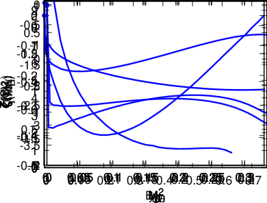
Figure 1: The function $\zeta$ plotted for $C$, $1-T$, $y_{3}$, $M_{\scriptscriptstyle\rm H}^{2}$, $M_{\scriptscriptstyle\rm D}^{2}$ and $B_{W}$.

With an angular-ordering argument, one can show that the limit $\zeta(v)$ for $v\to 0$ should tend to the corresponding two-jet limit values. In fact, in this limit, the emitted hard gluon becomes collinear to either the quark or the antiquark, let us say to the quark for sake of discussion, as shown in Fig. 2.

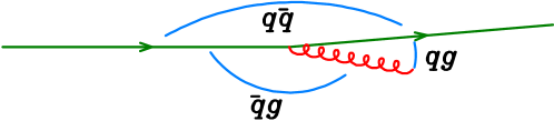
Figure 2: Dominant double logarithmic region near the two jet limit. The $qg$ dipole does not radiate, while the $q\bar{q}$ and $\bar{q}g$ dipoles differ only by their colour factor.

Because of coherence, the soft gluon associated with the power corrections sees the collinear quark-gluon pair as a single colour source, with the same colour of $q$. Thus the emission pattern is the same as that of a quark-antiquark pair. Alternatively, one may consider the emissions of the three dipoles $q\bar{q}$, $qg$, and $\bar{q}g$, that carry the colour factors $C_{\rm\scriptscriptstyle F}-C_{\rm\scriptscriptstyle A}/2$ for $q\bar{q}$ and $C_{\rm\scriptscriptstyle A}/2$ for $qg$ and $\bar{q}g$. The $qg$ dipole does not emit in the small angle limit (the eikonal formula vanishes there), and the $\bar{q}g$ dipole becomes equal to the $q\bar{q}$ dipole, giving $C_{\rm\scriptscriptstyle F}-C_{\rm\scriptscriptstyle A}/2+C_{\rm\scriptscriptstyle A}/2=C_{\rm\scriptscriptstyle F}$, i.e. the same soft radiation of a $q\bar{q}$ dipole. This must happen, however, when the logarithm of the shape variable is so large that it clearly prevails over single logs and constant terms. In the case of $C$ and $1-T$, one finds that for values of the shape variable $v\approx 10^{-3}$ the $\zeta$ function differs from the two-jet limit value by roughly 10%, i.e. of the order of $1/\log(v)$, that is the natural size of single-log corrections.

The case of $M_{\scriptscriptstyle\rm H}^{2}$ and $M_{\scriptscriptstyle\rm D}^{2}$, however, are much more extreme. In this case, in order to check that the two jet limit of $1$ and $0$ respectively are actually reached, we had to perform a dedicated calculation in quadruple precision in the small $v$ region. As an example, we show in Fig. 3 the result of this calculation for $M_{\scriptscriptstyle\rm H}^{2}$.

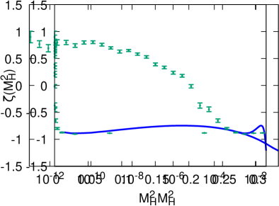
Figure 3: The $\zeta(M_{\scriptscriptstyle\rm H}^{2})$ function at very small value of its argument. The dots are obtained by performing a quadruple precision calculation and binning the results uniformly in a logarithmic scale. The left/right plot use a linear/logarithmic scale for the $x$ axis.

It is evident that $M_{\scriptscriptstyle\rm H}^{2}$ changes sign and reaches the value 1 very near zero, varying by about 2 units in a very narrow neighbourhood around zero. $M_{\scriptscriptstyle\rm D}^{2}$ undergoes an even stronger variation, changing by three units, and reaching zero from negative values. Such an abrupt change in the three-jet distribution as we approach the two-jet limit suggests that subleading soft terms in the two-jet limit remain more important than double logarithms all the way down to very small values of the shape variable, questioning on one side the possibility to associate the two-jet limit non-perturbative correction to the resummation of soft radiation, and, on the other side, the application of our newly computed non perturbative correction as we approach the two-jet limit.

4.4 Numerical checks

As a numerical check of the above calculations we also computed the $\zeta$ functions by directly generating the phase space comprising the three hard partons and the soft one, fixing its transverse momentum to a value $\lambda_{0}=Q_{0}/100$. More explicitly, we first generate the underlying Born momenta $p_{i}$, $i=1\ldots 3$, choose $\lambda_{0}=1$ GeV and $Q_{0}=100$ GeV, and construct the momentum of the radiated parton as in eqs. (16) to (17). Assuming for sake of argument that $p_{1}$ and $p_{2}$ are the momenta of the radiating dipole, we construct the recoil-corrected momenta as

$$P_{1} =p_{1}-l^{+}-\frac{1}{2}l_{\perp}\;,$$

$$P_{2} =p_{2}-l^{-}-\frac{1}{2}l_{\perp}\;.$$ (42)

In this way the total momentum is conserved, and the on-shell property of $P_{1/2}$ are maintained up to terms of order $\lambda^{2}/Q^{2}=1/10^{4}$. The event comprising $P_{1}$, $P_{2}$, $p_{3}$ and $l$ is then used to compute directly the values of the shape variables, and its difference with respect to the value obtained for momenta $p_{1}$, $p_{2}$ and $p_{3}$ is computed. Using this method, we find good agreement with the $\lambda\to 0$ calculations described in the previous section, except near the zero value of the shape variable and, in the case of the $C$ parameter, near the upper end-point of $3/4$, i.e. the 3-jet symmetric limit. We will make use of this method to give an estimate of corrections suppressed by higher powers of $\lambda$, as illustrated later.

5 Calculation of the observable distributions

We are interested in fitting $\alpha_{s}$ from event shapes in the three-jet region, where the novel results for the non-perturbative corrections can be used. Furthermore, in the three-jet region the relation between the observables and the value of $\alpha_{s}$ is more direct. For this reason, at the perturbative level we consider here only fixed-order predictions and, when determining the fit range, we will make sure that all-order resummed predictions, not included here, have a small effect.

Perturbative predictions for $e^{+}e^{-}\to 3$ jets are available up to next-to-next-to-leading order (NNLO) accuracy and are implemented in the public code EERAD3 Gehrmann-DeRidder:2007foh ; Gehrmann-DeRidder:2007vsv ; Gehrmann-DeRidder:2008qsl , which is based on the antenna subtraction formalism Gehrmann-DeRidder:2005btv and in a private code DelDuca:2016csb , which is based on the CoLoRFulNNLO subtraction method DelDuca:2016ily . We have used here predictions from EERAD3 up to NNLO and have checked that they agree with predictions using the CoLoRFulNNLO subtraction method up to NLO accuracy.

Denoting by $v$ a generic event shape, the normalized integrated distribution at center-of-mass energy $Q$ and at the renormalization scale $\mu_{R}$ can be written as

$$\Sigma_{\rm NNLO}(v) = \int_{0}^{v}dv^{\prime}\frac{1}{\sigma_{\rm\scriptscriptstyle NNLO}}\frac{d\sigma_{\rm\scriptscriptstyle NNLO}(v^{\prime},Q)}{dv^{\prime}}=\frac{\alpha_{s}(\mu_{\scriptscriptstyle\rm R})}{2\pi}\frac{dA(v)}{dv}$$ (43)

$$+ \left(\frac{\alpha_{s}(\mu_{\scriptscriptstyle\rm R})}{2\pi}\right)^{2}\frac{dB(v,x_{\mu_{\scriptscriptstyle\rm R}})}{dv}+\left(\frac{\alpha_{s}(\mu_{\scriptscriptstyle\rm R})}{2\pi}\right)^{3}\frac{dC(v,x_{\mu_{\scriptscriptstyle\rm R}})}{dv}\,,$$

where $x_{\scriptscriptstyle\rm R}=\mu_{\scriptscriptstyle\rm R}/Q$ and

$$B(v,x_{\mu_{\scriptscriptstyle\rm R}}) = B(v,1)+A(v)\left(\beta_{0}\ln x_{\scriptscriptstyle\rm R}-\sigma_{1}\right)\,,$$ (44)

$$C(v,x_{\mu_{\scriptscriptstyle\rm R}}) = C(v,1)+B(v,1)\left(2\beta_{0}\ln x_{\scriptscriptstyle\rm R}-\sigma_{1}\right)$$

$$+ A(v)\left(\frac{1}{2}\beta_{1}\ln x_{\scriptscriptstyle\rm R}+\beta_{0}^{2}\ln^{2}x_{\scriptscriptstyle\rm R}+\sigma_{1}^{2}-\sigma_{2}\right)\,,$$

with $\beta_{0}=(11C_{\rm\scriptscriptstyle A}-4n_{f}T_{R})/3$, $\beta_{1}=(34C_{\rm\scriptscriptstyle A}^{2}-20C_{\rm\scriptscriptstyle A}n_{f}T_{R}-12C_{\rm\scriptscriptstyle F}T_{R}n_{f})/3$, and where the expansion of the total cross section reads

$$\sigma_{\rm NNLO}=\sigma_{0}\left(1+\frac{\alpha_{s}(\mu_{\scriptscriptstyle\rm R})}{2\pi}\sigma_{1}+\left(\frac{\alpha_{s}(\mu_{\scriptscriptstyle\rm R})}{2\pi}\right)^{2}\sigma_{2}\right)\,,$$ (45)

with $\sigma_{1}=3C_{\rm\scriptscriptstyle F}/2$ and $\sigma_{2}=C_{\rm\scriptscriptstyle F}\left((123/8-11\zeta_{3})C_{\rm\scriptscriptstyle A}-3/8C_{\rm\scriptscriptstyle F}+(4\zeta_{3}-11/2)\,n_{f}\,T_{R}\right)$. For our central predictions we choose $x_{\scriptscriptstyle\rm R}=1/2$, and we estimate the error due to missing higher-order terms by varying this scale up and down by a factor of two. The choice of $x_{\scriptscriptstyle\rm R}=1/2$ for the central value is motivated by the fact that the scale entering in the production of the third jet is somewhat lower than $Q$.

The non-perturbative corrections discussed in Sec. 4 can be included as a shift in the argument of the cumulative cross section, i.e. according to eq. (38), but using instead the full NNLO cross section. We now depart from the large-$n_{f}$ parameterization of the shift, and switch instead to the dispersive model of ref. Dokshitzer:1998pt , where the role of the effective coupling of eq. (4) is played by a parameter $\alpha_{0}(\mu_{I}^{2})$. So, rather than using the definition of eqs. (40) and (41), the shift (see eq. (38)) can be written as

$$\delta v = \zeta(v){\cal M}\frac{\mu_{I}}{Q}\frac{4C_{\rm F}}{\pi^{2}}\Bigg{[}\alpha_{0}(\mu_{I}^{2})-\alpha_{s}(\mu_{R}^{2})-\alpha_{s}^{2}(\mu_{R}^{2})\frac{\beta_{0}}{\pi}\left(2\ln\frac{\mu_{R}}{\mu_{I}}+\frac{K^{(1)}}{2\beta_{0}}+2\right)$$ (46)

$$- \left.\alpha_{s}^{3}(\mu_{R}^{2})\frac{\beta_{0}^{2}}{\pi^{2}}\left(4\ln^{2}\frac{\mu_{R}}{\mu_{I}}+4\left(\ln\frac{\mu_{R}}{\mu_{I}}+1\right)\right)\times\left(2+\frac{\beta_{1}}{2\beta_{0}^{2}}+\frac{K^{(1)}}{2\beta_{0}}\right)+\frac{K^{(2)}}{4\beta_{0}^{2}}\right]\,,$$ (47)

where the observable dependent part $\zeta(v)$ has been discussed in detail in Sec. 4, the Milan factor is given in eq. (13) and $\alpha_{0}(\mu_{I}^{2})$ is defined as a mean value of the strong coupling in the CMW Catani:1990rr scheme below an infrared scale $\mu_{I}$ which is conventionally taken equal to 2 GeV:

$$\alpha_{0}(\mu_{I}^{2})=\frac{1}{\mu_{I}}\int_{0}^{\mu_{I}}d\mu\,\tilde{\alpha}_{s}(\mu^{2})\,,$$ (48)

where in the perturbative region the $\overline{\rm MS}$ and CMW couplings are related as

$$\tilde{\alpha}_{s}(\mu^{2})=\alpha_{s}(\mu^{2})\left(1+\frac{\alpha_{s}(\mu^{2})}{2\pi}K^{(1)}+\left(\frac{\alpha_{s}(\mu^{2})}{2\pi}\right)^{2}K^{(2)}+{\cal O}(\alpha_{s}^{3})\right)\,,$$ (49)

with Banfi:2018mcq ; Catani:2019rvy

$$K^{(1)} = C_{\rm\scriptscriptstyle A}\left(\frac{67}{18}-\frac{\pi^{2}}{6}\right)-\frac{5}{9}n_{f}\,,$$ (50)

$$K^{(2)} = C_{\rm\scriptscriptstyle A}^{2}\left(\frac{245}{24}-\frac{67}{9}\zeta_{2}+\frac{11}{6}\zeta_{3}+\frac{11}{5}\zeta_{2}^{2}\right)+C_{\rm\scriptscriptstyle F}n_{f}\left(-\frac{55}{24}+2\zeta_{3}\right)$$

$$+ C_{\rm\scriptscriptstyle A}n_{f}\left(-\frac{209}{108}+\frac{10}{9}\zeta_{2}-\frac{7}{3}\zeta_{3}\right)-\frac{1}{27}n_{f}^{2}+\frac{\beta_{0}}{2}\left(C_{\rm\scriptscriptstyle A}\left(\frac{808}{27}-28\zeta_{3}\right)-\frac{224}{54}n_{f}\right)\,.$$

The last terms in Eq. (47) are subtraction terms of contributions already accounted for in the perturbative calculation. This assumes that non-inclusive corrections are described by the same multiplicative Milan factor ${\cal M}$, that applies to all observables we consider with the exception of $y_{3}$, as discussed at the end of section 4.2.

Notice that in the large $n_{f}$ limit we found (see eq. (41))

$$\delta v=H_{\rm NP}\zeta(v)={\cal M}\times 4\frac{\alpha_{s}C_{\rm\scriptscriptstyle F}}{2\pi}\zeta(v)\times\frac{I_{\rm NP}}{Q},$$ (52)

where $I_{\rm NP}$ can be interpreted as the integral of the large-$n_{f}$, CMW effective coupling. In fact, expanding the second line of eq. (4) for small $\alpha_{s}$ we find

$$I_{\rm NP}=\frac{1}{\alpha_{s}(\mu)}\int_{0}^{\mu_{C}}\mathrm{d}\lambda\,\alpha_{s}(\lambda e^{-5/6}),$$ (53)

and

$$\alpha_{s}(\mu e^{-5/6})\approx\alpha_{s}(\mu)+\frac{5}{3}b_{0,n_{f}}\alpha_{s}(\mu)^{2}=\alpha_{s}(\mu)\left(1-\frac{5}{9}n_{f}\frac{\alpha_{s}(\mu)}{2\pi}\right),$$ (54)

consistently with eqs. (49) and (50).

However, formula (52) differs by a factor $\pi/2$ with respect to eq. (47), i.e. the factor $C_{\rm\scriptscriptstyle F}/(2\pi)$ is replaced by $C_{\rm\scriptscriptstyle F}/\pi^{2}$ in eq. (47). This replacement (for more details see ref. Dokshitzer:1998pt near formula (6.3)) is irrelevant for the purposes of this work, but we follow this prescription in order to fit values of $\alpha_{0}$ that can be compared to those found in previous publications.

It is possible to implement the non-perturbative corrections in different ways, leading to results that differ by terms of order ${\cal O}(\alpha_{s}/Q)$. We use this ambiguity to assign an uncertainty related to our treatment of non-perturbative corrections. For this purpose we define four schemes. Our default predictions, scheme “(a)”, are obtained by shifting the perturbative distribution $\Sigma_{\rm NNLO}(v)$ by the non-perturbative correction computed in Sec. 4

$$\Sigma^{(a)}(v)=\Sigma_{\rm NNLO}(v-\delta v)\,.$$ (55)

Furthermore, in scheme (a), we also add to $\delta v$ an approximate estimate of quadratic corrections. These are obtained from the difference between the numerical evaluation at finite transverse momentum described in Sec. 4.4 with respect to our standard calculation. More specifically, calling $\tilde{\zeta}(v)$ the evaluation of Sec. 4.4, we correct $\delta(v)$ as follows

$$\delta(v)=\zeta(v)H_{\rm NP}+\left(\tilde{\zeta}(v)\times\frac{Q_{0}}{\lambda_{0}}-\zeta(v)\right)\times\frac{Q_{0}}{\lambda_{0}}\times H_{\rm NP}^{2}\,.$$ (56)

Alternatively, instead of shifting the full NNLO distribution, one can shift only in the leading order term $\Sigma_{B}$ of the integrated distribution (scheme (b)):

$$\Sigma_{\rm\scriptscriptstyle FULL}^{(b)}(v)=\Sigma_{B}(v-\delta v)+\Sigma(v)-\Sigma_{B}(v)\,.$$ (57)

Yet another option is to expand the integrated distribution around the perturbative value (scheme (c)):

$$\Sigma_{\rm\scriptscriptstyle FULL}^{(c)}(v)=\Sigma(v)-\delta v\frac{\Sigma_{B}(v)}{dv}\,.$$ (58)

Scheme (d) is defined as scheme (a) but without the quadratic correction of eq. (56) included in the other schemes.

6 Fit to ALEPH data

We now compare the theoretical predictions including power corrections to the ALEPH data of ref. ALEPH:2003obs , where several shape variables were analyzed in the centre-of-mass energy range from 91.2 to 206 GeV. Here we focus upon the 91.2 GeV data. Including higher energy data does not lead to noticeable differences in the results, as we will discuss briefly in Sec. 7.1.

Our goal is to fit several observables at once. We need to select observables such that the power corrections in the three jet region can be computed with our methods, and that are at the same time available in ALEPH. These are the $C$-parameter, $\tau=1-T$, $y_{3}$ in the Durham scheme, the heavy-jet mass $M_{\scriptscriptstyle\rm H}^{2}$, the mass difference $M_{\scriptscriptstyle\rm D}^{2}$, and the wide jet broadening $B_{W}$. Since the $y_{3}$ variable is not really additive, we need to provide an estimate of the error associated with this. We will do so along the lines discussed at the end of Sec. 4.2.

The non-perturbative corrections to $M_{\scriptscriptstyle\rm H}^{2}$, $M_{\scriptscriptstyle\rm D}^{2}$ and $B_{W}$ have a common feature: in the 3-jet regime they differ drastically from their value in the two-jet limit. Such an abrupt change is quite worrisome, and may be taken as an indication that higher-order emissions may be associated with large corrections to the non-perturbative coefficient. For this reason, initially we leave these variables out of the fit, and only fit the $C$-parameter, $\tau$ and $y_{3}$. We fit the value of $\alpha_{s}(M_{\scriptscriptstyle\rm Z})$ and the non-perturbative parameter $\alpha_{0}$, defined in Sec. 5.

6.1 Treatment of uncertainties

6.1.1 Statistical and systematic errors, and correlations

The ALEPH data (available at the site https://www.hepdata.net/record/ins636645) includes statistical and systematic errors. Our method of choice for computing the error is the following. Calling $R_{i}$ the statistical error, $S_{i}$ the systematic error, $T_{i}$ the theoretical error relative to bin $i$, $C_{ij}$ the statistical correlation matrix, and ${\rm Cov}^{(\rm Sys)}_{ij}$ the covariance matrix for the systematic errors, we compute the full covariance matrix as

$$V_{ij}=\delta_{ij}(R_{i}^{2}+T_{i}^{2})+(1-\delta_{ij})C_{ij}R_{i}R_{j}+{\rm Cov}^{(\rm Sys)}_{ij}\,,$$ (59)

where the indices $i$ and $j$ run over all the bins of all observables that have been included in the fit. The ALEPH data quotes two kinds of systematic errors for the data taken at the $Z$ pole. We add these two errors in quadrature to obtain the global systematic error that we use in our analysis.

We computed the statistical correlation coefficients $C_{ij}$ using Pythia8. Calling $N_{i}$ and $N_{j}$ the number of events that fall into bin $i$ and bin $j$, and $N_{ij}$ the number of events that contribute to both bins, we have

$$C_{ij}=\frac{\frac{N_{ij}}{N}-\frac{N_{i}N_{j}}{N^{2}}}{\sqrt{\frac{N_{i}}{N}-\frac{N_{i}^{2}}{N^{2}}}\sqrt{\frac{N_{j}}{N}-\frac{N_{j}^{2}}{N^{2}}}},$$ (60)

where $N$ is the total number of events. Note that $N_{ij}$ is zero for different bins of the same observable, so that a negative correlation is expected for all pairs of bins in this case.

Statistical, systematic and theoretical errors are assumed to be uncorrelated among each other. For the covariance of the systematic errors we adopt the so called “minimum overlap” assumption (denoted in the following as MO), and set them equal to the minimum of the square of the systematic errors for the bins in question, i.e.

$${\rm Cov}^{(\rm Sys)}_{ij}=\delta_{ij}S_{i}^{2}+(1-\delta_{ij})\min(S_{i}^{2},S_{j}^{2})\,.$$ (61)

As an alternative, we computed the covariance matrix for the case of $C$, $T$ and $y_{3}$, by using the 24 systematic variations of the resulting distributions that were obtained by ALEPH in order to determine the systematic errors. We compute the covariance matrix and the central value as follows. We call $v^{(r)}_{i}$ the value of a shape variable for the bin $i$, where again $i$ denotes both the bin and the observable, and where $r$ labels the 25 replicas (a central value plus 24 variations.). We then define

$$\bar{v}_{i} =\frac{1}{N_{r}}\sum_{r}v^{(r)}_{i},$$ (62)

$$\bar{v}_{ij} =\frac{1}{N_{r}}\sum_{r}v^{(r)}_{i}v^{(r)}_{j},$$ (63)

$${\rm Cov}^{(\rm Sys)}_{ij} =\sum_{r}\left(v^{(r)}_{i}-\bar{v}_{i}\right)\left(v^{(r)}_{j}-\bar{v}_{j}\right)=N_{r}\left(\bar{v}_{ij}-\bar{v}_{i}\bar{v}_{j}\right)\,.$$ (64)

We use ${\rm Cov}^{(\rm Sys)}_{ij}$ as covariance matrix, and for the central value we use either the replica corresponding to the ALEPH default setup, or the average over all replicas $\bar{v}_{i}$. Some of the variations provided are double sided (i.e. they are associated with a positive and negative variation of a parameter). For these variations we have included a factor $1/2$ in the computation of $\bar{v}_{ij}$. In the following we call this the “replica method”, and denote it with R.

The covariance matrix is used to compute the $\chi^{2}$ value according to the standard formula

$$\chi^{2}=\sum_{ij}\left(v_{i}-v_{i}^{(\rm th)}\right)V_{ij}\left(v_{j}-v_{j}^{(\rm th)}\right).$$ (65)

6.1.2 Perturbative theory uncertainties

As a consequence of the high precision of the LEPI data, in order to obtain reasonable $\chi^{2}$ values when performing the fits we add the theoretical uncertainty in quadrature to the experimental one. We do not assume any correlations for the theoretical errors.

We define the perturbative theoretical error by considering three values for the renormalization scale: $Q$, $Q/2$ and $Q/4$. Calling $O(\mu_{\rm r})$ the value of a shape variable in a bin, we define the perturbative central value $O_{\rm cv}$ and the associated perturbative error $O_{\rm err}$ of the theoretical prediction as follows,

$$O_{\rm cv} =\frac{\max(O(Q),O(Q/2),O(Q/4))+\min(O(Q),O(Q/2),O(Q/4))}{2},$$ (66)

$$O_{\rm err} =\frac{\max(O(Q),O(Q/2),O(Q/4))-\min(O(Q),O(Q/2),O(Q/4))}{2}.$$ (67)

The perturbative theoretical error is quite small at the NNLO level we are working with.

6.1.3 Non-perturbative theory uncertainty

Non-perturbative corrections can be sizeable, up to the order of 10%, and thus we must also include an error associated with them. As seen in Sec. 4, there is evidence that power suppressed corrections of second order are not negligible, especially near the two jet region. We have estimated them and used them to correct the central value, see Eq. (56). We thus associated an uncertainty equal to twice the quadratic correction. As a further point, we expect that the $\zeta$ functions may receive perturbative corrections of order $\alpha_{s}\sim 0.1$. We thus define the following associated error to $\delta(v)$

$$\delta_{\rm err}(v)=2\cdot\left|\tilde{\zeta}(v)\times\frac{Q_{0}}{\lambda_{0}}-\zeta(v)\right|\times\frac{Q_{0}}{\lambda_{0}}\times H_{\rm NP}^{2}+0.1\cdot\delta(v)\,.$$ (68)

6.2 Correction for heavy-quark mass effects

Our NNLO calculation deals with massless quarks, while the data includes primary charm and bottom pairs. We correct the data by multiplying, for each bin of each observable denoted globally as $i$, the ratio of the Monte Carlo predictions for the corresponding observables $v_{i}$ evaluated without and with the $c$ and $b$ primary production processes

$$v_{i}^{\rm(corr)}=v_{i}\times\frac{v_{i}^{{\rm MC,}uds}}{v_{i}^{{\rm MC,}udscb}}.$$ (69)

The correction factors obtained using Pythia8 are shown in Fig. 4.

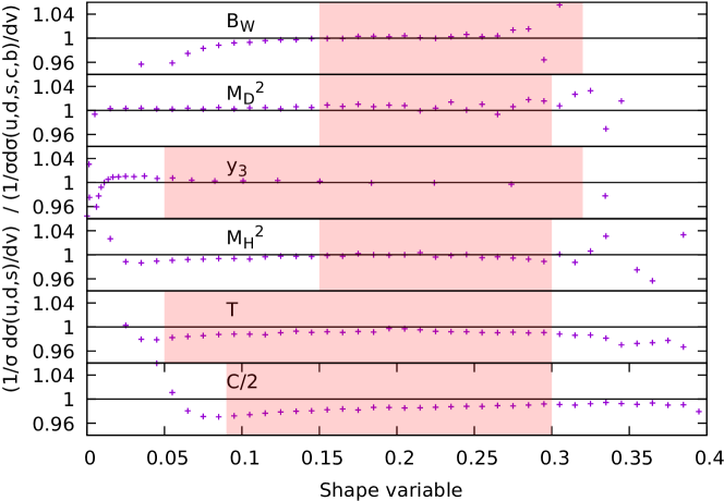
Figure 4: Heavy-flavours correction factors. The coloured band marks the range where fits are usually performed. Notice that we plot $C/2$ rather than $C$.

Notice that corrections are quite modest, although not totally negligible in some cases.

6.3 Hadron mass-effects corrections

As already discussed in Sec. 3, the theoretical calculation of shape-variable distributions deals with massless particles and the massless definition can be extended to deal with massive particles using different schemes. Since full particle identification is not available in an experimental context, this lack of information is filled by the Monte Carlo simulation when correcting from the detector level to the generator level. We also use a Monte Carlo generator to compute shape variables in the different schemes, and then construct migration matrices to correct from the scheme adopted by the experiment to any another scheme. More specifically, for each Monte Carlo event, we compute the shape variable in the standard scheme (the one adopted by the experiment, as defined in Sec. 2) and another scheme $S$. Assuming that the shape variable in the standard scheme falls into bin $i$, and the same shape variable in scheme $S$ falls into bin $j$, we increase by one unit a migration matrix $T_{ij}$. This matrix is used to correct the real data according to the formula

$$n_{j}^{\scriptscriptstyle(S)}=\sum_{i}n^{\scriptscriptstyle\rm(data)}_{i}\frac{T_{ij}}{\sum_{k}T_{ik}},$$ (70)

designed in such a way that if one replaces the $n^{\scriptscriptstyle(data)}_{i}$ with its Monte Carlo prediction, one obtains by construction the Monte Carlo prediction for $n_{j}^{\scriptscriptstyle(S)}$. In the following, we use this method to assess the hadron-mass sensitivity of our results.

7 Fit results

Our default fit is based on the ALEPH data of ref. ALEPH:2003obs at 91.2 GeV, and includes the thrust variable $\tau=1-T$, the $C$-parameter and the Durham 3-jet resolution variable $y_{3}$. In our perturbative predictions we fix the renormalization scale to $\mu_{R}=Q/2$. Non-perturbative effects are included as a shift of the total integrated distribution, corresponding to scheme (a) in Eq. (55). Our default mass scheme is the E scheme discussed in Sec. 3, since it yields intermediate results with respect to the other schemes, and is also closer to the result obtained in the standard scheme (i.e. the scheme used by ALEPH, as defined in Sec. 2). The treatment of correlations is described in Sec. 6.1.1. In particular, we chose the minimum-overlap method as our default choice, see Eq. (61). We apply the heavy-to-light correction factors described in Sec. 6.2 and illustrated in Fig. 4. We use Pythia8 as our standard Monte Carlo to compute the heavy-to-light correction factor and, when using a different mass scheme, to compute the migration matrix to be used to correct from the scheme adopted by the experiment to any another scheme. To perform our fit we use the default fit ranges listed in the second column of Table 1.

observable	default	Fit ranges (2)	Fit ranges (3)
$C$	[ 0.25 : 0.6 ]	[ 0.17 : 0.6 ]	[ 0.375 : 0.6 ]
$\tau$	[ 0.1 : 0.3 ]	[ 0.067 : 0.3 ]	[ 0.15 : 0.3 ]
$y_{3}$	[ 0.05 : 0.3 ]	[ 0.033 : 0.3 ]	[ 0.075 : 0.3 ]

Table 1: Default fit range used (second column), and alternative choices (obtained by multiplying the default lower bound by 2/3 and 3/2) used to estimate the impact of the choice of the fit range (third and forth column).

The lower edges of the ranges are determined in such a way that the impact of the resummation remains small (see Appendix A), while the upper edge is close to the three-particle kinematic bound of the observable. The result of the simultaneous fit of $\alpha_{s}$ and $\alpha_{0}$, together with the total $\chi^{2}$ and $\chi^{2}$ per degree of freedom is shown in the first line of Table 2.

Variation	$\alpha_{s}(M_{Z})$	$\alpha_{0}$	$\chi^{2}$	$\chi^{2}/N_{\rm deg}$
Default setup	0.1182	0.64	7.3	0.17
Renormalization scale $Q/4$	0.1202	0.60	9.1	0.21
Renormalization scale $Q$	0.1184	0.68	8.7	0.20
NP scheme (b)	0.1198	0.77	7.0	0.16
NP scheme (c)	0.1206	0.80	5.4	0.12
NP scheme (d)	0.1194	0.66	5.8	0.13
$P$-scheme	0.1158	0.62	10.7	0.24
$D$-scheme	0.1198	0.79	5.7	0.13
Standard scheme	0.1176	0.58	9.2	0.21
No heavy-to-light correction	0.1186	0.67	6.8	0.16
Herwig6	0.1180	0.59	15.9	0.36
Herwig7	0.1180	0.60	12.0	0.27
Ranges (2)	0.1174	0.62	12.7	0.23
Ranges (3)	0.1188	0.69	2.7	0.08
Replica method (around average)	0.1192	0.61	7.0	0.16
Replica method (around default)	0.1192	0.61	7.0	0.16
$y_{3}$ clustered	0.1174	0.66	8.2	0.19
$C$	0.1256	0.48	1.3	0.07
$\tau$	0.1194	0.64	0.8	0.04
$y_{3}$	0.1214	1.81	0.2	0.02
$C$, $\tau$	0.1238	0.51	2.6	0.07

Table 2: Default fit result for $\alpha_{s}(M_{Z})$ and $\alpha_{0}$ (first line) and other fit results obtained by varying the setup. See text for more details.

In the same table we illustrate how the fit results change if we vary any of the default choice made. In particular, we show the fit results when fixing the central value of the renormalization scale to $\mu_{R}=Q/4$ or $Q$. We investigate the impact of the way in which non-perturbative corrections are implemented, using the alternative schemes (b, c, d) presented in Sec. 5 (near Eq. (57)). We also present the result obtained using the $P$- and $D$- scheme to define the observables, as discussed in Sec. 6.3, and the result obtained in the standard scheme. To assess the impact of the heavy-to-light correction factor we switch it completely off. We vary the Monte Carlo used to compute the migration matrix for the scheme and the heavy-to-light correction factor, and consider Herwig6 Corcella:2000bw and Herwig7 Bellm:2015jjp . We vary the fit ranges adopted, as detailed in columns three and four of Table 1. Since correlations play an important role, we also use the replica method, see Eq. (64), using variations either around the average values of the replicas, or around the values of the default replica.

In the case of $y_{3}$ there is one further uncertainty, associated with the fact that we computed the non-perturbative correction assuming that the two soft partons from the splitting of the soft gluon are not clustered together. In order to estimate an associated uncertainty, we also computed the non-perturbative correction assuming that the two soft partons are always clustered together, see Eq. (37). The ratio of the latter to the former results ranges from $0.7$ up to $0.85$ in the fit window adopted for $y_{3}$. We have therefore performed the fit using alternatively the approximation where the soft partons are always clustered together. The corresponding result is reported in the table labeled as $y_{3}$-clustered. The central value for $\alpha_{s}$ in the simultaneous fit of $y_{3}$, $C$ and $T$ is reduced by 0.7%. Given the fact that we have chosen the lowest extreme of the variation, and that the correct result must lie between the always-clustered and the never-clustered cases, our estimate of this uncertainty is very conservative.

Finally, we examine how the fit results change if we consider one observable at the time, or if we exclude $y_{3}$ from the fits.

7.1 Including higher energy data

In the ALEPH publication ALEPH:2003obs , data are also available for centre-of-mass energies of 133, 161, 172, 183, 189, 200 and 206 GeV. Including these data does not appreciably change the result of the fit. For our default setup we get $\alpha_{s}(M_{\scriptscriptstyle\rm Z})=0.1184$ and $\alpha_{0}=0.64$, compared to $\alpha_{s}(M_{\scriptscriptstyle\rm Z})=0.1182$ and $\alpha_{0}=0.64$ of the fit on the $Z$ peak. We get a $\chi^{2}/N_{\rm deg}=0.70$, larger than the $0.17$ of the table. This is easily understood, since higher energy data have dominant statistical errors, and thus the $\chi^{2}/N_{\rm deg}$ is more in line with the expectation from statistical dominated data.

7.2 Discussion of the results

Our findings can be summarized as follows. For all results presented in the table, we observe an excellent $\chi^{2}$ of the fit. In particular the $\chi^{2}$ over number of degrees of freedom is always well below one. This is a consequence of our treatment of the theoretical error, that has been added bin-by-bin to the experimental one without correlations. Because of this, the theoretical prediction has considerable flexibility to adapt to data.

The choice of renormalization scale changes the fit by about 1.5%, the largest change driven by the variation to lower scales. A similar change can be observed when examining alternative schemes to implement non-perturbative corrections. The mass-scheme definitions bring in an effect of about 2%. The heavy-to-light correction factor changes $\alpha_{s}$ by just about one permille, hence the uncertainty associated to this correction seems negligible. A few permille differences are found when using a different Monte Carlo to change from the standard definition to the E-scheme and to perform the heavy-to-light correction. These small differences are not surprising since all the Monte Carlos we use are tuned to these data. The choice of the fit range has an impact on the result of about one percent. This confirms that the range chosen is such that the impact of the resummation is modest. The choice of how to treat statistical correlations has also a similar impact, and confirms that our minimal overlap approach provides a sensible description of the correlations. For $y_{3}$, the difference between the two limiting cases (where soft emissions are always-clustered or never-clustered) amounts also to about a one percent effect on the full fit.

Finally, we note that if one fits $\alpha_{s}$ and $\alpha_{0}$ from the three observables considered separately, one tends to get a larger value of the strong coupling, but with very different values of $\alpha_{0}$. Indeed, there is a tension in the fitted value of $\alpha_{0}$, where both thrust and $C$-parameter prefer a lower value, while $y_{3}$ prefers a higher one. When fitting all observables at the same time, the overall effect is that one finds an intermediate value for $\alpha_{0}$ and a lower value of $\alpha_{s}$. The $\chi^{2}$ of the fits remain excellent, which justifies a simultaneous fit. The role of each variable in the common fit is illustrated in Fig. 5.

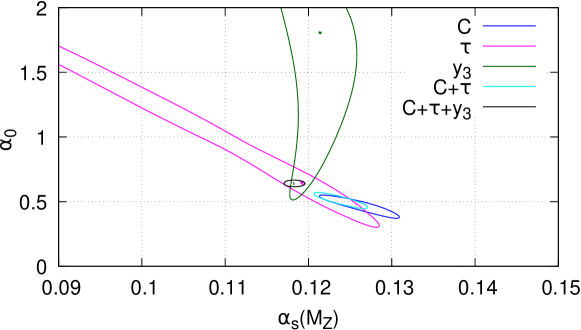
Figure 5: Contours at $\Delta\chi^{2}=1$ for fitting, $C$, $\tau$ and $y_{3}$ individually, and then in the combinations $C+\tau$ and $C+\tau+y_{3}$.

As one can see, for $C$ and $\tau$, $\alpha_{0}$ and $\alpha_{S}$ are strongly anti-correlated, and with a similar anti-correlation. On the other hand, $y_{3}$ has a $\zeta$ function that is small and of opposite sign, and thus $\alpha_{0}$ and $\alpha_{S}$ are only weakly correlated. The combined fit is then strongly constrained leading to an intermediate value of $\alpha_{0}$ and a smaller value of $\alpha_{s}$.

Altogether, we conclude by remarking that our fit results agree very well with the world average. In particular, we do not find low values of $\alpha_{s}$ for the thrust or $C$-parameter which are included in the current PDG average ParticleDataGroup:2020ssz . However, our results also clearly show that a fit of $\alpha_{s}$ from event shapes with an overall uncertainty below the percent level seems today not feasible. In particular, by changing certain choices that we have made, like the central renormalization scale or the mass scheme, one can easily obtain higher values of $\alpha_{S}$.

7.3 Comparison to results obtained by setting $\zeta(v)=\zeta_{\scriptscriptstyle 2J}(v)$

It is natural now to ask what the results of the fits would have been if we had used the non-perturbative correction as estimated in the two-jet limit. For $C$, $\tau$, $y_{3}$, $M_{\scriptscriptstyle\rm H}^{2}$ and $M_{\scriptscriptstyle\rm D}^{2}$ this amounts to setting the $\zeta(v)$ functions plotted in Fig. 1 to a constant value, according to the table 3. For $B_{W}$ the function $\zeta_{\scriptscriptstyle 2J}(v)$ can be found in Appendix F of ref. Dokshitzer:1998qp .

$v$	$C$	$\tau$	$y_{3}$	$M_{\scriptscriptstyle\rm H}^{2}$	$M_{\scriptscriptstyle\rm D}^{2}$	$B_{W}$
$\zeta_{\scriptscriptstyle 2J}(v)$	$3\pi$	$2$	$0$	$1$	$0$	App. F of Dokshitzer:1998qp

Table 3: The non-perturbative coefficients in the two jet limit.

The complete results are reported in table 4.

Variation	$\alpha_{s}(M_{Z})$	$\alpha_{0}$	$\chi^{2}$	$\chi^{2}/N_{\rm deg}$
Default setup	0.1132	0.55	15.8	0.36
Renormalization scale $Q/4$	0.1174	0.53	8.5	0.19
Renormalization scale $Q$	0.1126	0.57	22.0	0.50
NP scheme (b)	0.1126	0.63	25.7	0.58
NP scheme (c)	0.1134	0.72	16.4	0.37
NP scheme (d)	0.1132	0.55	15.8	0.36
$P$-scheme	0.1108	0.53	21.8	0.50
$D$-scheme	0.1126	0.66	16.1	0.37
Standard scheme	0.1134	0.51	15.9	0.36
No heavy-to-light correction	0.1130	0.58	15.9	0.36
Herwig6	0.1136	0.51	31.1	0.71
Herwig7	0.1136	0.52	21.8	0.49
Ranges (2)	0.1122	0.54	30.0	0.55
Ranges (3)	0.1134	0.58	10.5	0.33
Replica method (around average)	0.1158	0.53	13.4	0.31
Replica method (around default)	0.1160	0.53	13.5	0.31
$y_{3}$ clustered	0.1132	0.55	15.8	0.36
$C$	0.1238	0.45	1.3	0.08
$\tau$	0.1202	0.51	1.2	0.06
$y_{3}$	0.1160	–	1.4	0.18
$C$, $\tau$	0.1222	0.46	2.7	0.08

Table 4: Default fit result for $\alpha_{s}(M_{Z})$ and $\alpha_{0}$ (first line) and other fit results obtained by varying the setup, using the $\zeta_{\scriptscriptstyle 2J}$ values of table 3. See text for more details.

As shown there, the values of $\alpha_{s}$ found in this way are consistently lower than those of table 2. For example, for our default setup we have $\alpha_{s}(M_{\scriptscriptstyle\rm Z})=0.1182$ and $\alpha_{0}=0.64$, while using $\zeta_{\scriptscriptstyle 2J}$ we get $0.1132$ and $0.55$ respectively. On the other hand, the $\chi^{2}$ values are also quite acceptable.

A more detailed comparison of our default fit with the newly calculated $\zeta$ functions, and with the $\zeta_{\scriptscriptstyle 2J}$ functions corresponding to what has been available until now is shown in Fig. 6.

Figure 6: Central values and $\delta\chi^{2}=4$ (dashes) and 1 (solid) contours for our default fit of table 2 (blue) and the fit obtained with the $\zeta_{\scriptscriptstyle 2J}$ functions, corresponding to the default fit of table 4 (magenta).

As mentioned earlier, both fits look plausible, was it not for the fact that the $\zeta_{\scriptscriptstyle 2J}$ result favours values of $\alpha_{s}$ lower than the world average. The quality of the fits is displayed in Fig. 7.

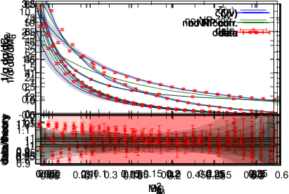
Figure 7: Theoretical predictions compared to data for our default setup on the left side, and the default setup with the $\zeta_{\scriptscriptstyle 2J}$ functions on the right side. The gray band represents the theoretical errors, while the red bars indicate the experimental ones, with the smaller one representing the statistical error, and the green lines show the pure perturbative results. The highlighted region represents the fit range.

As one can see, the fit with the full $\zeta(v)$ dependence seems slightly better, while the one with the $\zeta_{\scriptscriptstyle 2J}$ functions exhibits some tensions among the different observables. However, on the basis of the $\chi^{2}/N_{\rm deg}$ values, both fits are quite acceptable.

It is now interesting to see what happens to the remaining shape variables, $M_{\scriptscriptstyle\rm H}^{2}$, $M_{\scriptscriptstyle\rm D}^{2}$ and $B_{W}$ evaluated with the same parameters used for our default fits. The result is displayed in Fig. 8.

Figure 8: Theoretical predictions compared to data for our default setup on the left side, and the default setup with the $\zeta_{\scriptscriptstyle 2J}$ functions on the right side, for the $M_{\scriptscriptstyle\rm H}^{2}$, $M_{\scriptscriptstyle\rm D}^{2}$ and $B_{W}$ shape variables. The gray band represents the theoretical errors, while the red bars indicate the experimental ones, with the smaller one representing the statistical error. The green lines show the pure perturbative results.

There we see distinctly that the full $\zeta(v)$ fit works very well towards the three jet region for all the observables. The $\zeta_{\scriptscriptstyle 2J}$ fit, on the other hand, does not work in the three-jet limit, while its description of data improves in the two-jet region, with the noticeable exception of $M_{\scriptscriptstyle\rm D}^{2}$.

7.4 On the structure of $\alpha_{s}\lambda/Q$ corrections

Higher-order corrections to the linear $\lambda$ term are certainly present. The important issue is whether these corrections are of order $\alpha_{s}(Q)$ or rather $\alpha_{s}(\lambda)$. In this work we are implicitly assuming that they are suppressed by a power of $\alpha_{s}(Q)$. We do not have a solid argument to prove this assumption. However, by examining the structure of the linear power corrections near the two-jet limit we gain some insight into how this may actually work. In fact one can write schematically the correction of order $\lambda$ to a shape variable $v$ in the two-jet limit as

$$\left.\frac{\mathrm{d}\sigma}{\mathrm{d}v}\right|_{\rm\lambda}=N\lambda\left[\delta^{\prime}(v)\zeta_{\rm 2j}+(\delta^{\prime}(v)V_{1}+\delta(v)V_{2})\alpha_{s}+\frac{\mathrm{d}}{\mathrm{d}v}\left(\frac{\mathrm{d}\sigma_{q\bar{q}g}}{\mathrm{d}v}\zeta(v)\right)\right],$$ (71)

where the first term is the correction to the leading (two-parton) configuration, the second term is the virtual correction of order $\alpha_{s}$, and the third term is the correction we have computed, and where we implicitly assume some regularization of the $v\to 0$ region. The derivative of the delta function in the first term is necessary to guarantee that upon integration in $v$ there are no linear corrections left at order zero in $\alpha_{s}$, since we know that they are absent in the total cross section. The terms $V_{1}$ and $V_{2}$ incorporate corrections where the hard gluon is virtual and the gluer is real or virtual. In this case, besides the derivative of the $\delta$-function, we also include an explicit $\delta$-function to indicate that terms that do not vanish upon integration in $v$ must exist and are in fact divergent. We do not include virtual corrections to the $q\bar{q}g$ process for the exchange of a virtual gluon of mass $\lambda$, since it was shown in ref. Caola:2021kzt that these do not lead to linear terms in $\lambda$. The absence of linear corrections to the total cross section leads us to conclude that the integral of the above formula from $v=0$ up to any finite value of $v$ must be finite. In fact, if that was not the case, such divergence could not be canceled when performing the integral in the whole range of the shape variable. Thus the argument of $\alpha_{s}$ must be taken equal to the hard scale (that in this case is not quite $Q$, but is related to the typical transverse momentum of the perturbative gluon that sets the value of $v$). We have thus shown that the singular contributions of the hard gluon (hard relative to the scale $\lambda$) in the real emission and virtual exchanges cancel each other also in the coefficient of the linear term.

The argument given above also suggests a possible way to match the linear corrections in the three-jet limit to those in the two-jet limit, that are entangled with resummation effects. If we recall that the two-jet limit of the functions $\zeta(v)$ for $C$, $\tau$, $M_{\scriptscriptstyle\rm H}^{2}$ and $M_{\scriptscriptstyle\rm D}^{2}$ approach the value $\zeta_{\rm 2j}$, we could conclude that the part of the last term in the square bracket of eq. (71) that is singular in the two jet limit must combine with the virtual correction to yield a finite result. This combined result is precisely what one gets when expanding in powers of $\alpha_{s}$ the Sudakov form factor, including the shift for the two-jet non-perturbative correction. Thus, it is tempting to conclude that the singular part of the last term function should be combined with the resummation component of the cross section, while only the regular part should be applied to the 3-jet region. It is unlikely, however, that this approach will work for observables like $M_{\scriptscriptstyle\rm H}^{2}$ and $M_{\scriptscriptstyle\rm D}^{2}$, since in their case the limiting value is approached extremely slowly, and in the first case it has even opposite sign with respect to the average value of the $\zeta$ function in the fit range. It is however reassuring to see that if we restrict ourselves to regions far away the two-jet region, all shape variables are well described with the $\zeta$ functions computed here, while this is not the case with the values of table 3.

8 Conclusions

In this work, we study the effect of power corrections in $e^{+}e^{-}$ observables in comparison to data, under the light of the new findings of refs. Caola:2021kzt ; Caola:2022vea , where it was shown that power corrections can be computed directly in the three-jet configuration, rather than extrapolating them from the two-jet region. In refs. Caola:2021kzt ; Caola:2022vea these power corrections were computed for the $C$-parameter and for thrust. Here we also computed them for the three-jet resolution parameter in the Durham scheme $y_{3}$, for the squared mass of the heavy hemisphere $M_{\scriptscriptstyle\rm H}^{2}$, for the squared-mass difference of heavy-light hemispheres $M_{\scriptscriptstyle\rm D}^{2}$, and for the wide jet broadening $B_{W}$. The observables we considered are those that can be computed in the approach of refs. Caola:2021kzt ; Caola:2022vea , and that are included in the ALEPH data of ref. ALEPH:2003obs .

For simplicity we stick to a single data set, and we perform our calculation using the NNLO results for $e^{+}e^{-}$ hadronic observables, plus the newly computed power corrections. We do not attempt to include resummation effects. Rather, we stick to ranges of the observables that are far enough from the two jet region so that no visible depletion of the resummed result with respect to the fixed-order one is present.

We stress that in this work we are assuming that the non-perturbative corrections as estimated according to the results of ref. Caola:2021kzt ; Caola:2022vea are not drastically modified by the inclusion of soft radiation. Our argument concerning the two-jet limit region near eq. (71) seems to indicate that this is not the case. However, we are unable to provide a solid argument for the three-jet region.

Our main results can be summarized as follows. First of all, for all the shape variables that we considered, with the exclusion of the wide-jet broadening, the function that parameterised the non-perturbative correction, called $\zeta(v)$, approaches its two jet-limit value when its argument approaches the two-jet limit value (set conventionally to $v=0$), as one expects according to simple physics arguments. However, with the exception of $y_{3}$, the limit, is approached only for exponentially small values of the shape variable, so that, in practice, one sees an effective jump of the function near $v=0$. This jump is not very important for $C$ and for the thrust $\tau=1-T$, where it is around 10-20% of the two-jet limit value. It is instead quite large for $M_{\scriptscriptstyle\rm H}^{2}$ and $M_{\scriptscriptstyle\rm D}^{2}$, where it is such that the two-jet limit value cannot be considered representative of the value of the function even very close to the two-jet limit. In view of these observations, we exclude these observables from our fit, and also exclude $B_{W}$ that is positive and divergent in the two-jet limit, and is instead negative in the three-jet region.

We thus fitted $C$, $\tau$ and $y_{3}$, extracting a value for the strong coupling constant on the $Z$ peak, and for the non-perturbative parameter $\alpha_{0}$. The result of the fits yield a value of $\alpha_{s}$ in acceptable agreement with the world average, although we find that a number of variations of our procedure can lead easily to differences of the order of a percent. Using the same value of $\alpha_{s}$ and $\alpha_{0}$, we see that we can describe quite well also the remaining observables $M_{\scriptscriptstyle\rm H}^{2}$, $M_{\scriptscriptstyle\rm D}^{2}$ and $B_{W}$, as long as we remain far enough from the two-jet limit. Conversely, with the traditional implementation of power corrections, good fits to $C$, $\tau$ and $y_{3}$ can also be obtained, however the description of $M_{\scriptscriptstyle\rm H}^{2}$, $M_{\scriptscriptstyle\rm D}^{2}$ and $B_{W}$ in the three-jet region is totally unacceptable.

We stress again that the inclusion of resummation effects in the bulk of the three jet region leads smaller values of $\alpha_{s}$.

We are aware that the present work should only be considered as a preliminary exploration of the implications of the results of refs. Caola:2021kzt ; Caola:2022vea . In fact, there are few directions that need further exploration in order to fully exploit these new results.

First of all, it would be interesting and important to also include resummation effects in our analysis. Some ideas regarding this are discussed in the text, suggesting that perhaps the two-jet limit shift should be applied to the resummed component of the cross section, while the full $\zeta(v)$ dependent part should be applied to the finite part. Yet, whether this approach is sensible also when including resummation effects far from the two-jet region is a question that needs to be examined more closely, since for most observables $\zeta(0)$ differs considerably from $\zeta(v)$ in the three-jet region.

A second direction of improvement regards the choice of the hadron mass-scheme. Lacking a theoretically sound treatment of this problem, a possible development would be to see if there is a scheme that is preferred by data. This in turn would require considering enough observables that display different behaviour regarding the mass-scheme choice.

This brings us to consider a third extension of this work, which is to examine more variables, and find a sufficiently large set such that the requirements for the applicability of the results of refs. Caola:2021kzt ; Caola:2022vea are met, and such that their behaviour near the two-jet limit are closer to that of the thrust and the $C$-parameter. These new variables, could also be analyzed at present using preserved LEP data DPHEP:2015npg , while waiting for the beginning of operation of new $e^{+}e^{-}$ colliders.

A Impact of resummation

The fits of $\alpha_{s}$ carried out in this work rely on fixed order NNLO predictions, rather than on all-order (NNLL) predictions matched to fixed order, as computed in Ref. deFlorian:2004mp ; Becher:2008cf ; Monni:2011gb ; Chien:2010kc ; Becher:2010tm ; Becher:2012qc ; Alioli:2012fc ; Banfi:2014sua for event-shapes and in Ref. Banfi:2016zlc for the Durham three-jet resolution parameter $y_{3}$. Although it is customary to include resummation effects also far away from the two-jet region, in this work we made the assumption that resummation effects should not be included when the logarithm of the shape variable is not large. In order to determine a range for the fit, we thus compare in Fig. 9 NNLO and NNLO+NNLL predictions for the thrust variable $\tau=1-T$, the $C$-parameter, and the Durham three jet resolution variable $y_{3}$ and exclude in our fits the regions where matched predictions clearly depart from the fixed order. Each plot shows the ratio to the NLO prediction obtained with central renormalization scale $\mu_{R,0}=Q/2$. The green band shows the uncertainty of the NLO and the blue band of the NNLO, and are obtained by varying $\mu_{R}$ up and down by a factor two around the central value. For the NNLO+NNLL matched predictions we fix our default setup as follows: we set the central renormalization scale to $\mu_{R,0}=Q/2$, the resummation scale to $\mu_{Q,0}=Q/2$, we use the modified logarithm $L=1/p\ln\left(1/v^{p}-1/v_{\rm lim}^{p}+1\right)$, where $v_{\rm lim}$ denotes the kinematic limit of the event shapes, with p=3, and we use the log-R matching scheme (see e.g. ref. Banfi:2014sua ). The uncertainty band is then obtained as follows. Around the above described default setup, we vary, one at the time, $\mu_{R,0/2}\leq\mu_{R}\leq 2\mu_{R,0}$, $\mu_{Q,0}/2\leq\mu_{Q}\leq 2\mu_{Q,0}$, we vary $p$ to $p=2$ and $p=5$, and, finally, we use the R-matching scheme. This gives a total of eight matched predictions. The red uncertainty band shown in Fig. 9 is obtained by taking the envelope of all these predictions.

The onset of resummation effects is signalled both by a drop of the distribution of the resummed result and by an increase of the NLO result with respect to the NNLO one. We choose the lower bound of our fit ranges to be to the right of this region. Furthermore, for the three observables used in the fit we observe the following features: for the thrust, the uncertainty bands of the NNLO and matched predictions overlap, with the resummation band being a few percent higher, which would lead to slightly smaller values of $\alpha_{s}$. For the $C$-parameter one observes a somewhat similar behaviour. However, the difference between the center of the resummed and NNLO bands now reach up to 10% and the resummed band has a slightly different shape compared to the NNLO one. For $y_{3}$ one observes small effects, at the level of a 2%, however in this case the uncertainty bands do not overlap since the NNLO band is extremely small. From all three plots it is also clear that the difference between NNLO and matched predictions does not vanish even for large values of the observables. This is due to the fact that, even with the modified logarithms, the resummation is not switched off fast enough even close to the end-point of the distributions.

From the figures it can be seen that in the case of the thrust, the resummed prediction seems to follow the trend of the NLO and NNLO corrections, possibly approximating higher-order results if they follow the same trend. However, in the case of the $C$-parameter the resummed result has a slope that is not present in the NLO and NNLO results. Furthermore, in the case of $y_{3}$, the trend is to have the NNLO distribution smaller than the NLO one, while the resummed result is larger. In conclusion, although it has become common practice, we see no reason in principle to include resummation effects also in the three-jet region.

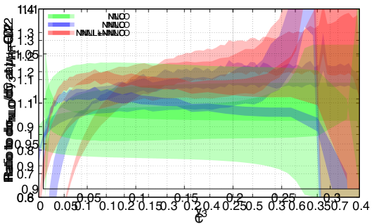
Figure 9: Comparison between NLO (green bands), NNLO (blue bands) and NNLO+NNLL (red bands) predictions for the thrust (left), $C$-parameter (central), $y_{3}$ (right). See text for more details.

References

- (1) A. Gehrmann-De Ridder, T. Gehrmann, E. W. N. Glover and G. Heinrich, Infrared structure of e+ e- — 3 jets at NNLO, JHEP 11 (2007) 058, [0710.0346].
- (2) A. Gehrmann-De Ridder, T. Gehrmann, E. W. N. Glover and G. Heinrich, NNLO corrections to event shapes in e+ e- annihilation, JHEP 12 (2007) 094, [0711.4711].
- (3) A. Gehrmann-De Ridder, T. Gehrmann, E. W. N. Glover and G. Heinrich, Jet rates in electron-positron annihilation at O(alpha(s)**3) in QCD, Phys. Rev. Lett. 100 (2008) 172001, [0802.0813].
- (4) V. Del Duca, C. Duhr, A. Kardos, G. Somogyi and Z. Trócsányi, Three-Jet Production in Electron-Positron Collisions at Next-to-Next-to-Leading Order Accuracy, Phys. Rev. Lett. 117 (2016) 152004, [1603.08927].
- (5) S. Catani, L. Trentadue, G. Turnock and B. R. Webber, Resummation of large logarithms in e+ e- event shape distributions, Nucl. Phys. B 407 (1993) 3–42.
- (6) S. Catani and B. R. Webber, Resummed C parameter distribution in e+ e- annihilation, Phys. Lett. B 427 (1998) 377–384, [hep-ph/9801350].
- (7) Y. L. Dokshitzer, A. Lucenti, G. Marchesini and G. P. Salam, On the QCD analysis of jet broadening, JHEP 01 (1998) 011, [hep-ph/9801324].
- (8) A. Banfi, G. P. Salam and G. Zanderighi, Semi-numerical resummation of event shapes, JHEP 01 (2002) 018, [hep-ph/0112156].
- (9) P. F. Monni, T. Gehrmann and G. Luisoni, Two-Loop Soft Corrections and Resummation of the Thrust Distribution in the Dijet Region, JHEP 08 (2011) 010, [1105.4560].
- (10) A. Banfi, H. McAslan, P. F. Monni and G. Zanderighi, A general method for the resummation of event-shape distributions in annihilation, JHEP 05 (2015) 102, [1412.2126].
- (11) Z. Tulipánt, A. Kardos and G. Somogyi, Energy–energy correlation in electron–positron annihilation at NNLL + NNLO accuracy, Eur. Phys. J. C 77 (2017) 749, [1708.04093].
- (12) A. Banfi, H. McAslan, P. F. Monni and G. Zanderighi, The two-jet rate in at next-to-next-to-leading-logarithmic order, Phys. Rev. Lett. 117 (2016) 172001, [1607.03111].
- (13) T. Becher and M. D. Schwartz, A precise determination of from LEP thrust data using effective field theory, JHEP 07 (2008) 034, [0803.0342].
- (14) Y.-T. Chien and M. D. Schwartz, Resummation of heavy jet mass and comparison to LEP data, JHEP 08 (2010) 058, [1005.1644].
- (15) T. Becher and G. Bell, NNLL Resummation for Jet Broadening, JHEP 11 (2012) 126, [1210.0580].
- (16) T. Becher, G. Bell and M. Neubert, Factorization and Resummation for Jet Broadening, Phys. Lett. B 704 (2011) 276–283, [1104.4108].
- (17) G. Dissertori, A. Gehrmann-De Ridder, T. Gehrmann, E. W. N. Glover, G. Heinrich, G. Luisoni and H. Stenzel, Determination of the strong coupling constant using matched NNLO+NLLA predictions for hadronic event shapes in e+e- annihilations, JHEP 08 (2009) 036, [0906.3436].
- (18) OPAL collaboration, G. Abbiendi et al., Determination of using OPAL hadronic event shapes at - 209 GeV and resummed NNLO calculations, Eur. Phys. J. C71 (2011) 1733, [1101.1470].
- (19) JADE collaboration, S. Bethke, S. Kluth, C. Pahl and J. Schieck, Determination of the Strong Coupling alpha(s) from hadronic Event Shapes with O(alpha**3(s)) and resummed QCD predictions using JADE Data, Eur. Phys. J. C64 (2009) 351–360, [0810.1389].
- (20) G. Dissertori, A. Gehrmann-De Ridder, T. Gehrmann, E. W. N. Glover, G. Heinrich and H. Stenzel, Precise determination of the strong coupling constant at NNLO in QCD from the three-jet rate in electron–positron annihilation at LEP, Phys. Rev. Lett. 104 (2010) 072002, [0910.4283].
- (21) JADE collaboration, J. Schieck, S. Bethke, S. Kluth, C. Pahl and Z. Trocsanyi, Measurement of the strong coupling from the three-jet rate in annihilation using JADE data, Eur. Phys. J. C73 (2013) 2332, [1205.3714].
- (22) A. Verbytskyi, A. Banfi, A. Kardos, P. F. Monni, S. Kluth, G. Somogyi, Z. Szőr, Z. Trócsányi, Z. Tulipánt and G. Zanderighi, High precision determination of from a global fit of jet rates, JHEP 08 (2019) 129, [1902.08158].
- (23) A. Kardos, S. Kluth, G. Somogyi, Z. Tulipánt and A. Verbytskyi, Precise determination of from a global fit of energy–energy correlation to NNLO+NNLL predictions, Eur. Phys. J. C78 (2018) 498, [1804.09146].
- (24) R. Akhoury and V. I. Zakharov, On the universality of the leading, 1/Q power corrections in QCD, Phys. Lett. B 357 (1995) 646–652, [hep-ph/9504248].
- (25) Y. L. Dokshitzer, G. Marchesini and B. R. Webber, Dispersive approach to power behaved contributions in QCD hard processes, Nucl. Phys. B 469 (1996) 93–142, [hep-ph/9512336].
- (26) Y. L. Dokshitzer, A. Lucenti, G. Marchesini and G. P. Salam, Universality of 1/Q corrections to jet-shape observables rescued, Nucl. Phys. B 511 (1998) 396–418, [hep-ph/9707532].
- (27) Y. L. Dokshitzer, A. Lucenti, G. Marchesini and G. P. Salam, On the universality of the Milan factor for 1 / Q power corrections to jet shapes, JHEP 05 (1998) 003, [hep-ph/9802381].
- (28) R. A. Davison and B. R. Webber, Non-Perturbative Contribution to the Thrust Distribution in e+ e- Annihilation, Eur. Phys. J. C59 (2009) 13–25, [0809.3326].
- (29) T. Gehrmann, G. Luisoni and P. F. Monni, Power corrections in the dispersive model for a determination of the strong coupling constant from the thrust distribution, Eur. Phys. J. C73 (2013) 2265, [1210.6945].
- (30) M. Beneke, Renormalons, Phys. Rept. 317 (1999) 1–142, [hep-ph/9807443].
- (31) G. P. Korchemsky and G. F. Sterman, Power corrections to event shapes and factorization, Nucl. Phys. B 555 (1999) 335–351, [hep-ph/9902341].
- (32) G. P. Korchemsky and S. Tafat, On power corrections to the event shape distributions in QCD, JHEP 10 (2000) 010, [hep-ph/0007005].
- (33) C. W. Bauer, C. Lee, A. V. Manohar and M. B. Wise, Enhanced nonperturbative effects in Z decays to hadrons, Phys. Rev. D 70 (2004) 034014, [hep-ph/0309278].
- (34) C. Lee and G. F. Sterman, Momentum Flow Correlations from Event Shapes: Factorized Soft Gluons and Soft-Collinear Effective Theory, Phys. Rev. D 75 (2007) 014022, [hep-ph/0611061].
- (35) C. W. Bauer, S. Fleming, D. Pirjol and I. W. Stewart, An Effective field theory for collinear and soft gluons: Heavy to light decays, Phys. Rev. D 63 (2001) 114020, [hep-ph/0011336].
- (36) C. W. Bauer, D. Pirjol and I. W. Stewart, Soft collinear factorization in effective field theory, Phys. Rev. D 65 (2002) 054022, [hep-ph/0109045].
- (37) R. Abbate, M. Fickinger, A. H. Hoang, V. Mateu and I. W. Stewart, Thrust at N3LL with Power Corrections and a Precision Global Fit for alphas(mZ), Phys. Rev. D83 (2011) 074021, [1006.3080].
- (38) A. H. Hoang, D. W. Kolodrubetz, V. Mateu and I. W. Stewart, Precise determination of from the -parameter distribution, Phys. Rev. D91 (2015) 094018, [1501.04111].
- (39) G. Luisoni, P. F. Monni and G. P. Salam, -parameter hadronisation in the symmetric 3-jet limit and impact on fits, Eur. Phys. J. C 81 (2021) 158, [2012.00622].
- (40) F. Caola, S. Ferrario Ravasio, G. Limatola, K. Melnikov and P. Nason, On linear power corrections in certain collider observables, JHEP 01 (2022) 093, [2108.08897].
- (41) F. Caola, S. Ferrario Ravasio, G. Limatola, K. Melnikov, P. Nason and M. A. Ozcelik, Linear power corrections to shape variables in the three-jet region, 2204.02247.
- (42) ALEPH collaboration, A. Heister et al., Studies of QCD at e+ e- centre-of-mass energies between 91-GeV and 209-GeV, Eur. Phys. J. C 35 (2004) 457–486.
- (43) Y. L. Dokshitzer, G. Marchesini and G. P. Salam, Revisiting nonperturbative effects in the jet broadenings, Eur. Phys. J. direct 1 (1999) 3, [hep-ph/9812487].
- (44) G. P. Salam and D. Wicke, Hadron masses and power corrections to event shapes, JHEP 05 (2001) 061, [hep-ph/0102343].
- (45) V. Mateu, I. W. Stewart and J. Thaler, Power Corrections to Event Shapes with Mass-Dependent Operators, Phys. Rev. D 87 (2013) 014025, [1209.3781].
- (46) G. E. Smye, On the 1/Q correction to the C - parameter at two loops, JHEP 05 (2001) 005, [hep-ph/0101323].
- (47) S. Ferrario Ravasio, P. Nason and C. Oleari, All-orders behaviour and renormalons in top-mass observables, JHEP 01 (2019) 203, [1810.10931].
- (48) M. Dasgupta and Y. Delenda, On the universality of hadronisation corrections to QCD jets, JHEP 07 (2009) 004, [0903.2187].
- (49) A. Gehrmann-De Ridder, T. Gehrmann and E. W. N. Glover, Antenna subtraction at NNLO, JHEP 09 (2005) 056, [hep-ph/0505111].
- (50) V. Del Duca, C. Duhr, A. Kardos, G. Somogyi, Z. Szőr, Z. Trócsányi and Z. Tulipánt, Jet production in the CoLoRFulNNLO method: event shapes in electron-positron collisions, Phys. Rev. D 94 (2016) 074019, [1606.03453].
- (51) S. Catani, B. R. Webber and G. Marchesini, QCD coherent branching and semiinclusive processes at large x, Nucl. Phys. B 349 (1991) 635–654.
- (52) A. Banfi, B. K. El-Menoufi and P. F. Monni, The Sudakov radiator for jet observables and the soft physical coupling, JHEP 01 (2019) 083, [1807.11487].
- (53) S. Catani, D. De Florian and M. Grazzini, Soft-gluon effective coupling and cusp anomalous dimension, Eur. Phys. J. C 79 (2019) 685, [1904.10365].
- (54) G. Corcella, I. G. Knowles, G. Marchesini, S. Moretti, K. Odagiri, P. Richardson, M. H. Seymour and B. R. Webber, HERWIG 6: An Event generator for hadron emission reactions with interfering gluons (including supersymmetric processes), JHEP 01 (2001) 010, [hep-ph/0011363].
- (55) J. Bellm et al., Herwig 7.0/Herwig++ 3.0 release note, Eur. Phys. J. C 76 (2016) 196, [1512.01178].
- (56) M. Cacciari, G. P. Salam and G. Soyez, The anti- jet clustering algorithm, JHEP 04 (2008) 063, [0802.1189].
- (57) Particle Data Group collaboration, P. A. Zyla et al., Review of Particle Physics, PTEP 2020 (2020) 083C01.
- (58) DPHEP collaboration, S. Amerio et al., Status Report of the DPHEP Collaboration: A Global Effort for Sustainable Data Preservation in High Energy Physics, 1512.02019.
- (59) D. de Florian and M. Grazzini, The Back-to-back region in e+ e- energy-energy correlation, Nucl. Phys. B 704 (2005) 387–403, [hep-ph/0407241].
- (60) T. Becher and M. Neubert, Drell-Yan Production at Small , Transverse Parton Distributions and the Collinear Anomaly, Eur. Phys. J. C 71 (2011) 1665, [1007.4005].
- (61) S. Alioli, C. W. Bauer, C. J. Berggren, A. Hornig, F. J. Tackmann, C. K. Vermilion, J. R. Walsh and S. Zuberi, Combining Higher-Order Resummation with Multiple NLO Calculations and Parton Showers in GENEVA, JHEP 09 (2013) 120, [1211.7049].