PISN-explorer: hunting the descendants of very massive first stars

Abstract

The very massive first stars ($m>100$ $\rm M_{\odot}$) were fundamental to the early phases of reionization, metal enrichment, and super-massive black hole formation. Among them, those with $140\leq\rm m/\rm M_{\odot}\leq 260$ are predicted to evolve as Pair Instability Supernovae (PISN) leaving a unique chemical signature in their chemical yields. Still, despite long searches, the stellar descendants of PISN remain elusive. Here we propose a new methodology, the PISN-explorer, to identify candidates for stars with a dominant PISN enrichment. The PISN-explorer is based on a combination of physically driven models, and the FERRE code; and applied to data from large spectroscopic surveys (APOGEE, GALAH, GES, MINCE, and the JINA database). We looked into more than 1.4 million objects and built a catalogue with 166 candidates of PISN descendants. One of which, 2M13593064+3241036, was observed with UVES at VLT and full chemical signature was derived, including the killing elements, Cu and Zn. We find that our proposed methodology is efficient in selecting PISN candidates from both the Milky Way and dwarf satellite galaxies such as Sextans or Draco. Further high-resolution observations are highly required to confirm our best selected candidates, therefore allowing us to probe the existence and properties of the very massive First Stars.

1 Introduction

The first (Pop III) stars formed out of primordial composition gas, i.e. in environments where the fragmentation process was less efficient then in local star-forming regions, thus enabling the formation of more massive stars than those that we observe today: from a few tens, up to thousands of solar masses (e.g. Susa et al., 2014; Hirano et al., 2015). Their characteristic mass, furthermore, was likely $\geq 10$ $\rm M_{\odot}$ (e.g. Bromm, 2013). These theoretical findings have strong physical grounds and have been reported across decades by means of different analytical calculations (see e.g. Silk, 1977; McKee & Tan, 2008), numerical simulations (see e.g. Abel et al., 2002; Hosokawa et al., 2011), and studies of stellar archaeology (e.g. Ishigaki et al., 2018; Rossi et al., 2021). According to cosmological models, these primitive stars were likely hosted by the bulge and the stellar halo of the Milky Way (see e.g. Tumlinson, 2010; Salvadori et al., 2010; Starkenburg et al., 2017a) and by Local group dwarf galaxies (e.g. Salvadori et al., 2015). From an observational point of view, however, we are still lacking key probes of first stars in the high-mass regime ($\rm m_{*}>140$ $\rm M_{\odot}$) very recently some indirect hints have been provided (Pagnini et al. sumbitted).

Very massive first stars, $140\leq\rm m_{*}/M_{\odot}\leq 260$, are predicted to end their lives as energetic Pair Instability Supernovae (PISN), which inject $50\%$ of their mass in the form of metals into the interstellar medium (ISM). Thus, a single PISN will strongly enrich the primordial gas with a probability distribution function peaking at $\mathrm{[Fe/H]\approx-2.0}$ (Karlsson et al., 2008; de Bennassuti et al., 2017; Salvadori et al., 2019), leaving a unique chemical signature with a strong odd-even effect (e.g. Heger & Woosley, 2002; Takahashi et al., 2018). Unfortunately, pure PISN descendants are predicted to be extremely rare: even at the peak metallicities, $\mathrm{[Fe/H]\approx-2.0}$, they are thought to represent $<0.1\%$ of Milky Way stars (de Bennassuti et al., 2017). The traditional approach of searching only for stars showing 100% PISN enrichment has thus not proven successful. Rather, a large fraction of PISN descendants are expected to also have a significant contribution from normal Pop II stars, which can form early on in the Pop III-enriched ISM and then evolve as core-collapse supernovae (CCSN).

The abundances of the so-called killing elements Cu and Zn (Salvadori et al., 2019) may be the smoking gun for a true PISN descendant. These elements are barely produced by PISNe, but yielded by all other supernovae (see also Vanni et al. in prep). The extreme sub-solar abundances of Zn and Cu with respect to Fe from PISNe, persist even in environments polluted by other sources up to a $50\%$ level (Salvadori et al., 2019). But given the rarity of such stars, until now, only two descendants of PISN have been reported (Aoki et al., 2014; Salvadori et al., 2019). We are thus in the situation where even a few more identified PISN descendants would greatly advance the field.

In the recent years there has been a breakthrough in large spectroscopic surveys targeting stars in and around the Milky Way (e.g. Gaia, APOGEE, GALAH, GES). Millions of stars have been observed with intermediate- to high-resolution spectra ($R\gtrsim 10,000$), and these numbers will further increase with two large upcoming spectroscopic surveys, starting operations in the next two years: WEAVE in the Northern hemisphere (Dalton et al., 2016), and 4MOST in the South (de Jong et al., 2019). For the first time, we are thus able to have the statistics to identify and characterise rare populations, such as PISN descendants.

Searching through such large databases, however, requires a focused and dedicated effort, and with this goal in mind we have developed an innovative methodology, the PISN-explorer. With a combination of theoretical models (Salvadori et al., 2019), and the FERRE code (Allende Prieto et al., 2006), the PISN-explorer exploits all the chemical abundances measured by large surveys (e.g. APOGEE, GALAH, GES, or MINCE) to identify stars that have likely been dominantly enriched by PISN ($\gtrsim 50\%$). Here we present this new method, allowing us for the first time to use large databases of chemical abundances to systematically search for the elusive PISN descendants.

2 The theoretical models

The models used by the PISN-explorer are adopted from the general parametric study presented in Salvadori et al. (2019). This study provides predictions for the chemical properties of an ISM predominantly imprinted by very massive first stars exploding as PISNe, i.e. where the PISNe products account for $\geq 50\%$ of metals in the ISM. The model is general because it condenses the unknown physical processes related to early cosmic star-formation, metal diffusion, and mixing, into three free parameters: 1) the star formation efficiency, $f_{*}$, which provides the fraction of ISM gas condensed into stars; 2) the dilution factor, $f_{\rm dil}$, which parametrises the amounts of metals effectively retained into the ISM; 3) and the mass fraction of ISM metals contributed by PISNe, $f_{\rm PISN}$. Predictions for a PISN-imprinted ISM are provided by exploring the full parameter space. Hence the predictions are general and essentially model independent.

The ansatz of this approach is to assume that a single very massive first star exploding as PISN can form in the primordial star-forming (mini-)haloes. This assumption is strongly supported by the results of hydrodynamical cosmological simulations following the formation of the first stars (e.g. Hirano et al., 2014). The chemical enrichment of the ISM is evaluated after the injection of metals by a single PISN ($f_{\rm PISN}=100\%$) with different progenitor masses, $m_{\rm PISN}=[140-260]\mathrm{M}_{\odot}$. It turns out that the final metallicity (or [Fe/H]) of the ISM is settled by the PISN mass and by the ratio between the star-formation efficiency and the dilution factor, $f_{*}/f_{\rm dil}$. Furthermore, it is always $Z_{\rm ISM}>10^{-3}\rm Z_{\odot}$, which implies that “normal” Pop II stars can form out of this medium and thus contribute to the subsequent ISM enrichment (see Fig. 2 of Salvadori et al. 2019).

The abundance ratios of each element X (from C to Zn) with respect to iron, are computed by varying the relative contribution of PISN and Pop II stars to the chemical enrichment ($f_{\rm PISN}=[50-100]\%$) and by assuming that Pop II stars form according to a standard Larson Initial Mass Function (IMF): $\phi(m_{\star})=m^{-2.35}_{\star}exp(-m_{ch}/m_{\star})$ with $m_{ch}=0.35\rm M_{\odot}$ (Larson, 1998). The calculations are made by adopting the yields by Heger & Woosley (2002) for very massive first stars exploding as PISNe, ${\rm{Y^{\rm PISN}_{\rm X}}}(m_{\rm PISN})$, and of Woosley & Weaver (1995) for Pop II stars with initial masses $m_{*}=[8-40]\mathrm{M}_{\odot}$ and metallicities, $Z_{*}=[10^{-4};1]\mathrm{Z}_{\odot}$, which explode as CCSN, ${\rm Y_{X}}^{\rm II}(m_{*},Z_{*})$. According to Woosley & Weaver (1995) we assume that stars between 40 and 140 $\rm M_{\odot}$ collapse directly into a black hole thus not contributing to the chemical enrichment. Note that since we are integrating over the entire Pop II IMF the derived yields are not so different from those obtained with models assuming that $m_{*}>20\rm M_{\odot}$ stars produce a negligible amount of heavy elements (e.g. Limongi & Chieffi, 2018). Salvadori et al. (2019) demonstrated that the ISM abundance ratios, [X/Fe], or the chemical abundance pattern of the stars formed out of it, depend upon $f_{\rm PISN}$, the yields of PISN and of Pop II stars; but they are not directly affected by $f_{*}/f_{\rm dil}$ although this ratio controls the metallicity of the Pop II stars contributing to the ISM enrichment.

Figure 1: Example of the PISN-explorer analysis performed on an APOGEE star.

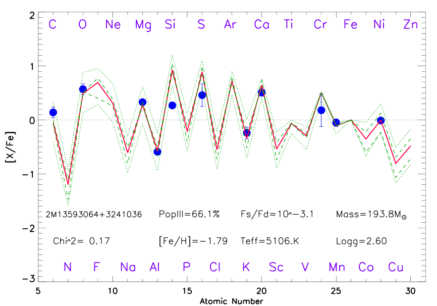
(a) The measured chemical signature of 2M13593064+3241036 from APOGEE (blue dots) together with the best fit to a PISN model computed with the PISN-explorer (red line). Derived PISN parameters and main stellar parameters are also shown. Finally, for comparison we show interpolated models with $\pm 20\rm M_{\odot}$ of PISN mass (dotted lines) and $\pm 15\%$ of PISN contamination (dashed lines).

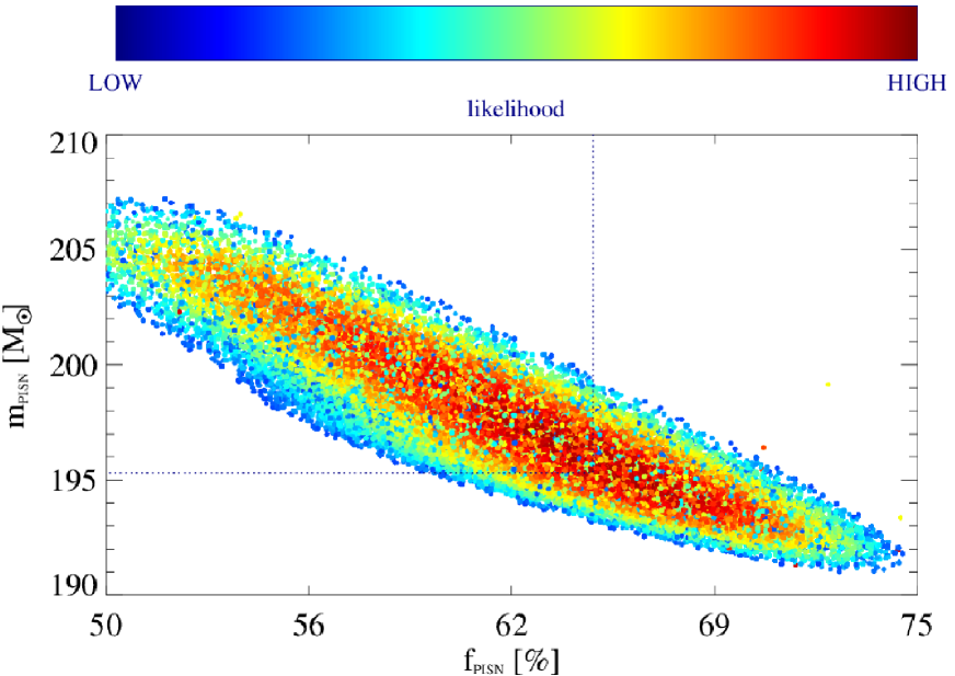
(b) $f_{\rm PISN}-m_{\rm PISN}$ space of solutions when applying and MCMC algorithm computed with FERRE over the chemical signature of 2M13593064+3241036 including 10 chains of 50,000 experiments each. Color bar represents the likelihood of each solution.

3 Exploited datasets

The goal of this work is to efficiently select candidates for PISN descendants from existing and publicly available data. Suitable databases should provide reliable elemental abundances for FGK stars together with stellar parameters: effective temperature, surface gravity, and metallicity ($T_{\mathrm{eff}}$, $\log g$, and [Fe/H]). From the available spectroscopic surveys, we restrict our selection to the large surveys that have the best chemical abundances information (APOGEE, GALAH, Gaia-ESO, and the MINCE survey). In addition, we exploit high-quality literature data available through the JINA database. Here, we will mainly focus on elements from C to Zn but sometimes abundances of heavier elements (Ba, Ce) could be also used to impact the selection, since these are expected to be low in PISN descendants. Finally, in the following we assumed the solar abundances each survey used at that time. Future -improved- measurements of solar abundances are easily applicable to our methodology.

3.1 APOGEE

The Apache Point Observatory Galactic Evolution Experiment 2 (APOGEE-2; Majewski et al., 2017) is a near-infrared high-resolution survey in the $H$-band (1.514-1.696 $\rm\mu m$ at $R\sim 22,500$) that provides stellar parameters ($T_{\mathrm{eff}}$, $\log g\,\,$, [Fe/H]), radial velocities, and elemental abundances. Solar abundances are those from Asplund et al. (2005). The high quality of APOGEE measurements at metallicities down to $\rm[Fe/H]\sim-2$ clearly recommends the use of this spectroscopic survey. For our purpose, we use the final allStar catalogue of APOGEE Data Release (DR) 17 (Abdurro’uf et al., 2022) which includes up to 20 elemental abundances (C, N, O, Na, Mg, Al, Si, P, S, K, Ca, Sc, Ti, Cr, Mn, Fe, Co, Ni, Cu, and Ce) for 879,437 spectra (733,901 objects). Following the recommendation of the APOGEE team, we discard both Ti i and Ti ii from further analysis. Unfortunately, the Cu absorption lines in the infrared are extremely week and therefore only detectable for metal-rich stars, $\rm[Fe/H]>-1$.

3.2 GALAH

The GALactic Archaeology with HERMES (GALAH, De Silva et al., 2015) survey is a large spectroscopic survey in the optical at a resolving power $R\sim 28,000$, covering four wavelength windows within 4713 to 7887 Å. The third data release (DR3; Buder et al., 2021), including the main_allspec_v2 catalogue, provides for 588,571 stars: stellar parameters, radial velocities, and chemical abundances for up to 30 elements (Li, O, C, Na, Mg, Al, Si, K, Ca, Sc, Ti, V, Cr, Mn, Co, Ni, Cu, Zn, Rb, Sr, Y, Zr, Mo, Ru, Ba, La, Ce, Nd, Sm, Eu). GALAH provides chemical abundances at $\rm[Fe/H]\gtrsim-2$, but not all elements are available at the lowest metallicities. Solar abundances are from Grevesse et al. (2007).

3.3 Gaia-ESO

The Gaia-ESO Survey (GES, Gilmore et al., 2012, 2022) has observed 115,000 stars from the main components of the Milky Way, including star clusters, using FLAMES at the VLT. The employed instruments (GIRAFFE and UVES) provide high-resolution spectra, $16,200<\rm R<47,000$, covering various wavelength ranges, depending on the configuration. We retrieved the latest available DR5 (Randich et al., 2022) with 114,324 stars. The solar abundances used for this survey are those from Asplund et al. (2009). A significant fraction of GES pointings is dominated by metal-rich stars $\rm[Fe/H]>-1$, which are less likely to be PISN descendants. These fields can, however, also contain some metal-poor stars, so we included the entire dataset. Including the entire GES sample also ensures that our search is as unbiased as possible. The GES DR5 dataset includes stellar parameters, radial velocities, and chemical abundances for up to 31 elements (He, Li, C, N, O, Na, Mg, Al, Si, S, Ca, Sc, Ti, V, Cr, Mn, Co, Ni, Cu, Zn, Sr, Y, Zr, Mo, Ba, La, Ce, Pr, Nd, Sm, Eu)

3.4 MINCE

Measuring at Intermediate metallicity Neutron-Capture Elements (MINCE, Cescutti et al., 2022) is a project aiming to study abundances for neutron-capture elements using different facilities such as HARPS, UVES, or FIES. Conveniently, the targets selection is designed to observe intermediate and very metal-poor stars ($\rm-0.7\gtrsim[Fe/H]\gtrsim-2.5$). For this work we employed the first year sample including 43 stellar targets and high quality elemental abundances O, Na, Mg, Al, Si, S, Ca, Sc, Ti, V, Cr, Mn, Co, Ni, Cu, Zn. The employed solar abundances are those from Lodders et al. (2009) and Caffau et al. (2011) for O and S. The following data releases in subsequent years will be a valuable source of PISN descendant candidates.

3.5 JINA

The Joint Institute for Nuclear Astrophysics (JINA) database (Abohalima & Frebel, 2018) is a collection of literature papers with high-resolution analysis of 1658 metal-poor stars $\rm[Fe/H]<-2$, including a variable range of elemental abundances (from Li to U). We downloaded the whole database, set the solar abundances to Asplund et al. (2009), and treat each entry in the same way regardless of its origin (e.g. halo, bulge, or dwarf galaxy members).

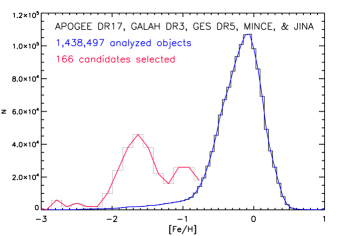
Figure 2: Metallicity distribution functions for the 1.4 million stars analysed (blue), and the 166 PISN selected candidates (red). Note that the red distribution has been arbitrarily scaled for easier comparison.

4 Methodology

We have developed the PISN-explorer, a systematic methodology to efficiently select PISN-polluted candidates from observational data (Sec. 3) using the FERRE code from Allende Prieto et al. (2006) and theoretical predictions from Salvadori et al. (2019) (Sec. 2). FERRE is a FORTRAN code optimised for spectral analysis (e.g. Allende Prieto et al., 2014; Aguado et al., 2017) but capable of performing fitting of any class of data to a rectangular grid of theoretical models. The PISN-explorer methodology implies several steps:

1. Packaging of models: A grid of theoretical predictions for the chemical abundances of PISN descendants (50-100% PISN pollution) is created with a FERRE-friendly header. Key information included in the header: a) the number and label for each free parameter included in the models ($f_{\rm PISN}$, ${\log_{10}{(f_{*}/f_{\rm dil}})}$, and $m_{\rm PISN}$); b) the minimum value for each parameter (0.5, -4, and 140 $\rm M_{\odot}$ respectively); c) the steps for each parameter (0.1, 1, 9$\rm M_{\odot}$, respectively); d) the number of elements (“pixels”) within the models (25, counting from C to Zn), and their atomic numbers (“$\lambda$-array”). Finally, the grid is complete with the predictions ($\rm[X_{i=6,30}/Fe]$) in rows just below the header. Here, as explained in Sec. 2, we use Pop II yields from (Woosley & Weaver, 1995) to be fully consistent with Salvadori et al. (2019). However, if the potential user of PISN-explorer wishes to use a different set of models (e.g. Nomoto et al., 2013; Limongi & Chieffi, 2018, or any other that can be published in the future) the grid has to be re-computed as explained along these lines.
   

2. Preparing the data: Following the recommendation of each survey, we discard stars with suboptimal flags, STAR_BAD ASPCAPFLAG for APOGEE and flag_sp$\neq 0$ for GALAH, while all the sample was taken from Gaia-ESO, MINCE, and JINA. Additionally, we only considered elemental abundances with x_fe_flag $=0$ in both APOGEE and GALAH, meaning that only reliable values are considered. For each star in our sample we prepared three different files with 25-columns length each: 1) the measured chemical ratios ($\rm[X_{i=6,30}/Fe]_{obs}$) from C to Zn; 2) the uncertainties ($\sigma_{\rm[X_{i=6,30}/Fe]_{obs}}$); and 3) the weight we gave to each measurement ($\omega_{\rm[X_{i=6,30}/Fe]_{obs}}$). The $\omega$ values are equal to 0 if there is no measurement for element X, 1 for Cu and Zn, and 0.5 for the rest. Thus, we give double weight to the killing elements since they are the smoking gun of PISN pollution. This tuning implies that the $\chi^{2}_{0}$ will heavily depend on the Cu and Zn if they are available but no effect otherwise.
   

3. Launching the code: FERRE is able to look for the best fit by interpolating between the nodes of the grid. We used quadratic interpolation and Nash’s truncated Newton algorithm (Nash & Sofer, 1990). After the minimum $\chi^{2}{0}$ is found, the code produces the set of best parameters with errors, along with an interpolated model. In Fig. 1(a) we show an example of a fit with the observed values $(\rm[X_{i=6,30}/Fe]_{obs}$, blue dots) from the literature for a single APOGEE object, and the best fit $(\rm[X_{i=6,30}/Fe]_{fit}$, red line) derived with FERRE, giving a set of parameters: $f_{\rm PISN}=66.1$%; $f_{*}/f_{\rm dil}=10^{-3.1}$; and $m_{\rm PISN}=193.8\rm M_{\odot}$. We also calculated a reduced $\chi^{2}$ as $\chi^{2}=\chi^{2}_{\circ}/(N-M)$, where $\chi_{\circ}^{2}$ is the one defined in Equation 14 of Salvadori et al. (2019), N the number of fitting points, and M the number of free parameters of the model. Therefore, we will have reduced $\chi^{2}$ values $>0$. In the following we will refer to this reduced $\chi^{2}$.
   

4. Interpreting the results and caveats: The results of the PISN-explorer are interpreted, i.e. the best set of parameters ($f_{\rm PISN}$, ${\log_{10}{(f_{*}/f_{\rm dil}})}$, and $m_{\rm PISN}$), and an interpolated model ($\rm[X_{i=6,30}/Fe]_{fit}$). When a star’s chemical signature is very far from the theoretical predictions (the vast majority of the cases), the code will not be able to find a good fit and will usually end up on a solution with a high $\chi^{2}$ at the limit of the grid ($m_{\rm PISN}=140$ $\rm M_{\odot}$, for example). This is because the code is trying to find something beyond the ranges of the grid, and should therefore be interpreted as a non-reliable solution. Unless the quality of the fit is very high, solutions with $f_{\rm PISN}$ and $m_{\rm PISN}$ close to the limit of the grid are discouraged. However, the ${\log_{10}{(f_{*}/f_{\rm dil}})}$ parameter is less sensitive to model-to-model variations because the predicted abundance patterns do not directly depend upon this quantity (see Sec. 2). Therefore good fits can appear at the limits of the ${\log_{10}{(f_{*}/f_{\rm dil}})}$ range. Objects with a very low number of derived elemental abundances ($\leq 5$) lead to no recommended solutions. Additionally, there are some elements that are more affected by stellar processes in evolved stars. C, for instance, is converted into N during the CN cycle, and brought to the surface during the red giant branch phase. Thus, it is highly recommended to correct for these stellar evolutionary effects (see, e.g. Placco et al., 2014). Finally, any available corrections due to inhomogeneities in the three-dimensional (3D) stellar atmosphere and the non-local thermodynamic equilibrium (NLTE) state of the matter for elemental abundances will significantly improve the results of the analysis.
   

5. Looking for asymmetric signatures: The well known odd-even bias is a remarkable feature of measured stellar chemical compositions (see, e.g. Payne, 1925; Russell, 1941). Elements with an even atomic number (C, O, Mg, Si, Ca, Ti) are more easily detected in the atmospheres of metal-poor stars and therefore most of the surveys are able to provide them for a large number of objects with good precision. Consequently, the available chemical signatures are asymmetric, i.e. biased towards even-elements. This is unfortunate, since a stark contrast between the abundances of odd and even elements is a key signature of PISN yields (see e.g. 1(a)). Therefore, the higher is the number of available odd elemental abundances the better performance can be obtained with this methodology.
   

6. MCMC validation: To ensure that degeneracy in the parameters determination is not affecting our methodology we used a Markov-Chain Monte-Carlo (MCMC) analysis based on self-adaptive randomised subspace sampling (Vrug et al., 2009). This algorithm is also implemented in the FERRE code and can help to understand the solution space, and offer a statistical validation for the evaluation of uncertainties. We launched 10 chains of 50,000 experiments each and let the code burn up to 500 experiments in each chain. In Fig. 1(b) we show the likelihood in the $f_{\rm PISN}-m_{\rm PISN}$ space of solutions. Although the employed algorithm looking for the best solution is different, unsurprisingly the best solution is compatible within the uncertainties with the one shown in Fig. 1(a) ($f_{\rm PISN}=65$%; $f_{*}/f_{\rm dil}=10^{-3.1}$; and $m_{\rm PISN}=195.3$ $\rm M_{\odot}$). The likelihood distribution (Fig. 1(b)) shows solution areas with similar probability that are smaller than the step of the grid. Furthermore, the smooth behaviour of the likelihood distribution shows that no evident degeneracies are playing a critical role in our calculations. Therefore, this MCMC test demonstrates that the solution FERRE is finding is stable and the nodes corresponding to the space parameters are small enough to account for the required sensitivity.

5 Target Selection

Our sample mainly consists of nearby stars from the disk, the bulge, and the halo of the Milky Way (Sec. 3). We analyzed 1,438,497 stars following the methodology explained in Sec. 4 with no further cuts applied at this stage. In Fig. 2 we show in blue the metallicity distribution function of the whole sample, including GALAH, APOGEE, GES, and JINA stars with available measurements of chemical abundances. The target selection based on the PISN-explorer analysis is a two step procedure based first on hard cuts applied blindly over the entire sample, systematic selection, and secondly on more specific and survey-dependent selection, individual selection. We finally end up with our golden catalogue of candidates for further high-resolution follow-up. The three stages are detailed below:

• Systematic Selection. The MDF for the entire considered sample is shown in red in Fig. 2. Following the known caveats (discussed in Sec. 4), we discarded objects with less than 5 available chemical abundances. In addition, since we focus on FGK type metal-poor stars we only include stars with $4000$ K$<$$T_{\mathrm{eff}}$ $<7000$ K and $\rm[Fe/H]$ $<-0.7$. Hotter stars have much weaker metallic absorption lines, and it is in general not possible to derive a complete chemical signature. On the other hand, the early M type stars are dominated by molecular bands, and thus cooler stars would also prevent from determining accurate chemical abundances. The remaining sample of 385202 stars is run through the PISN-explorer. Subsequently, we discard fits with $\chi^{2}>0.35$ and remove out after inspection solutions with $m_{\rm PISN}<145\rm M_{\odot}$ and/or $f_{\rm PISN}<55$% since they are close to the limit of the grid.

• Individual Selection. Hard cuts themselves do not guaranty an optimal selection. First of all, the killing elements, Cu and Zn are important guidelines and, if available, we discard objects with $\rm[Cu,Zn/Fe]>0$. In addition, we maximised, when possible, odd-even effect by selecting objects with $\rm[Mg/Al]>0.7$. We also preferred objects with $\rm[Mg/Ca]<0.0$ that is also a desirable sign according to our models. After applying all of this criteria we end-up in a catalogue of 166 candidates from all included surveys (Sec. 3). In Fig. 2 we also show in red our selection. It is quite clear that different datasets contribute in a different manner. While the most metal-poor bump ($\rm[Fe/H]\lesssim-2.5$) is mainly from the JINA database, the most metal-rich peak ($\rm[Fe/H]\approx-1$) is dominated by GES stars. However, the bulk of our selection based on GALAH and APOGEE is peaked at $\rm[Fe/H]=-1.7$, close to the most likely metallicity region where PISN descendants are predicted to live (e.g. Karlsson et al., 2008; Salvadori et al., 2019). We note that the red MDF showed in Fig. 2 is, at first order, independent of the selection criteria we applied.

• Golden catalogue We included extra criteria before consider any star for future follow-up. At this stage more careful direct inspection is recommended, analysing the suitability of each candidate individually. Therefore, we included two objects that did not completely achieve the general criteria $\chi^{2}<0.35$ but have $\rm[Zn/Fe]<-0.8$. In addition to it, we removed objects with clear s-process enrichment (Ba or Ce) to discard possible contribution from AGB stars. In addition to it, to select objects with large number of abundances (N$\geq 10$) is obviously a desirable strategy so we prioritise those to others with better fit but less complete chemical information. Finally, we also include suitable observability cuts (V${}_{mag}\leq$ 16) ending up in a 45 objects golden catalogue that contains the most promising candidates to be enriched by PISN pollution.

Following the selection criteria described in this section we ended up with our golden catalogue of 45 objects. One of the most promising candidates, 2M13593064+3241036 from APOGEE, is shown in Fig. 1(a). For this object the quality of the fit is remarkable: measurements for two odd elements were available (Al and K), and the odd-even effect is clear, $\rm[Mg/Al]=+0.92$, $\rm[Mg/Ca]<-0.18$, and $\rm[Ca/K]<+0.75$ . APOGEE does provide NLTE corrections for Mg, K, and Ca (Osorio et al., 2020). Unfortunately, APOGEE does not measure Zn and provides very few Cu abundance measurements. Thus, the smoking gun of PISN pollution is missing for this interesting star. Therefore, we applied for an ESO-DDT proposal of one hour to try to accurately measure both killing elements, Zn and Cu.

6 Observations and Analysis

6.1 UVES observations

Our target, 2M13593064+3241036, was observed with UVES at the 8.2 m VLT Kueyen Telescope in a single observing block (OB) of one hour in service mode, during the night of the 28th of March 2022, under program ID 108.23N5.001. A $1\aas@@fstack{\prime\prime}2$ slit was used with $1\times 1$ binning in grey sky conditions and an airmass of $\sim 2.0$. The seeing was $1\aas@@fstack{\prime\prime}2$ after corrected by airmass. Our settings used dichroic $\#Dic1\,(390+564)$ and provided a spectral coverage between 330 and 660 nm. We corrected each spectrum for the barycentric velocity. The signal-to-noise ratio (SNR) per pixel in the spectra was $\sim$19 at 390 nm, 48 at 510 nm, and 55 at 660 nm. The resolving power for this set up is R$\sim 45,000$ for the blue part of the spectrum ($330-452$ nm) and R$\sim 41,500$ for the red ($480-680$ nm). The data were reduced using the REFLEX environment (Freudling et al., 2013) within the ESO Common Pipeline Library.

6.2 Stellar Parameters

APOGEE analysis pipeline (ASPCAP; García Pérez et al., 2016) used spectral profile fitting to derive for 2M13593064+3241036: $T_{\mathrm{eff}}$ =5106 K, $\log g\,\,$=2.60, and $\rm[Fe/H]$ $=-1.79$ (Majewski et al., 2017). We perform a similar analysis for our UVES optical spectrum by fitting the data with the FERRE. FERRE is able to match observations with a library of stellar models by interpolating between the nodes of the grid for different parameters. The synthetic models were computed originally by Aguado et al. (2021), covering the following range of parameters:

• $4500~{}\mathrm{K}<T_{\mathrm{eff}}<7000~{}\mathrm{K}$, $\Delta T_{\mathrm{eff}}=250~{}\mathrm{K}$

• $1.0<\log g\,\,<5.0$, $\Delta\log g\,\,=0.5$

• $-4.0<\rm[Fe/H]<+1.0$, $\Delta\rm[Fe/H]=0.5$

• $-1.0<\rm[C/Fe]<+3.0$, $\Delta\rm[C/Fe]=1.0$

The models were computed in one dimension local thermodynamical equilibrium (1D-LTE) with the ASSET code and the ATLAS12 stellar atmospheres (Sbordone et al., 2007; Kurucz, 2005). The atomic and molecular data were taken from Kurucz webpage and enriched with the literature as explained in (Allende Prieto et al., 2018). For the analysis we first smoothed and resampled the models to the UVES resolution and performed a running-mean normalization with a 150-pixel window. Then we also normalised the data accordingly and launched the code with the Nash’s truncate Newton search algorithm (Nash & Sofer, 1990), and cubic order interpolation. Thus we derived for 2M13593064+3241036: $T_{\mathrm{eff}}$ $=5036\pm 105$ K, $\log g\,\,$$=2.59\pm 0.20$, $\rm[Fe/H]$ $=-2.29\pm 0.10$, and $\rm[C/Fe]$$=+0.05\pm 0.15$. Atmospheric parameters are in excellent agreement with those derived from the H-band, however, the measured [Fe/H] is 0.5 dex lower than the ASPCAP value. This discrepancy is certainly unusual and cannot be easily explained since the APOGEE spectrum is of high quality (SNR$\sim$130). We re-analysed the APOGEE spectrum with consistent models from Allende Prieto et al. (2018) and found compatible metallicity $\rm[Fe/H]\sim-1.9$. Therefore, we attribute the discrepancy to a problem that could be related with a problem to the sky or background subtraction in the APOGEE spectrum. Additionally, we found persisting_high flag (residual signal in the detector) within ASPCAP documentation that, in principle, giving the brightness of this object should not be a problem. Yet, we argue that it could possibly play a role and contribute to explain such a difference. Unfortunately, the impact of this metallicity discrepancy significantly influences the abundances, [X/Fe], derived by APOGEE for this star, as is shown in the following Sec. 6.3. Thus, for sake of caution we will not use APOGEE abundances for this object.

As sanity check, we compared our stellar parameters from spectroscopy with the ones we derived with the Gaia colours (Gaia Collaboration et al., 2021), applying the calibration by Mucciarelli et al. (2021) and assuming $\rm[Fe/H]=-2.3$, $T_{\mathrm{eff}}$ $=5144\pm 100$ K and $\log g\,\,$$=2.5\pm 0.2$. Both set of parameters are in good agreement also with the APOGEE ones. Furthermore, we note that in different visits APOGEE finds different radial velocities: MJD 56389: -15.6
,km s^-1; MJD 56405: -9.3 km s^-1; and MJD 56412 -8.8 km s^-1 with S/N > 30 for all visits. In addition, Gaia RVS (Cropper et al., 2018) is giving $v_{rad}=-13.5\pm 3.2\rm\,km\,s^{-1}$ with 38 transits. Finally, from the UVES spectrum we derive $v_{rad}=-15.8\pm 1.2\rm\,km\,s^{-1}$. Therefore we cannot exclude that this star is a binary system.

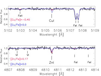
Figure 3: UVES spectrum (black lines) of the star 2M13593064+3241036, around the absorption lines: Cu i at 5105 Å (top); and Zn i at 4810 Å (bottom). Two models at different elemental abundances are also shown (blue and red lines). Other metallic absorption lines in the spectra are also labelled.

Table 1: Stellar parameters, abundances, ratios, errors and number of detected lines for individual species derived in 2M13593064+3241036 from UVES and APOGEE data.

Gaia DR2 id 1457695618046140800
$\rm RA(deg)=209.877547$, $\rm DEC(deg)=32.684315$
$v_{rad}=-13.45$ km s-1, $T_{\mathrm{eff}}=5035$ K, $\log g\,\,$=2.59
Species	$\log\epsilon$ (X)${}_{\odot}^{1}$	$\log\epsilon$ (X)	$\mbox{[X/Fe]}^{2}$	$\sigma_{\mbox{[X/Fe]}}$	$N$	$\mbox{[X/Fe]}_{\rm NLTE}$
C (CH)	8.39		0.05	0.11	–
N (CN)	7.78		<0.10	–	–
O i	8.66		1.103	0.15	2
Na i	6.17	4.22	0.36	0.12	2	$-$0.13
Mg i	7.53	5.77	0.28	0.09	9	0.28
Al i	6.37	3.86	$-$0.20	0.11	2	0.06
Si i	7.51	5.48	0.40	0.10	1	0.34
K i	5.08	5.08	0.243	0.10	1
Ca i	6.31	4.53	0.39	0.12	12	0.49
Sc ii	3.05	0.87	$-$0.07	0.08	3
Ti i	4.90	3.10	$-$0.19	0.23	4
Ti ii	4.90	3.01	$-$0.05	0.08	16	$-$0.12
V i	4.00	1.85	$-$0.02	0.08	8
Cr i	5.64	3.23	$-$0.27	0.11	6
Mn i	5.39	2.68	$-$0.25	0.08	3
Fe i	7.45	5.31	$-$2.314	0.06	231	$-$2.27
Fe ii	7.45	5.16	$-$2.385	0.09	7
Co i	4.92	2.83	0.08	0.12	6
Ni i	6.23	3.84	$-$0.37	0.13	5
Cu i	4.21	–	<$-$0.40	–	–
Zn i	4.60	3.84	0.17	0.13	2
Sr ii	2.92	0.12	0.12	0.09	2
Y ii	2.21	0.63	$-$0.63	0.09	4
Zr ii	2.59	0.24	0.24	0.09	3
Ba ii	2.17	0.13	0.13	0.10	3
Eu ii	0.52	0.55	0.03	0.10	2
1Solar abundances adopted from Asplund et al. (2005)
2LTE and NLTE ratios are referred to [Fe/H]LTE and [Fe/H]NLTE.
3Abundance derived from the APOGEE spectrum and not used here.
4[Fe/H] from Fe i is given instead of [X/Fe]
4[Fe/H] from Fe ii is given instead of [X/Fe]

6.3 Elemental abundances

Detailed chemical abundances analysis has also been performed taking advantage of the FERRE code. First, we identified all the resolved lines present in the UVES spectrum and measure their central wavelength by using splot routine within IRAF (Tody, 1993). Secondly, we built for each chemical species a FERRE-readable mask that includes all the observed lines. These spectral windows include the vast majority of the information of each elemental abundance. Thirdly, we fixed the stellar parameters to the values derived in the Sec. 6.2 and launched FERRE again leaving only as a free parameter the chemical abundances. The code calculates and averages the abundance of each element and gives the associated uncertainty. The result of this analysis is presented in Table 1, and summarised in the following subsections.

6.3.1 CNO-elements

The carbon abundance is derived, as explained in Sec. 6.2, by using specific models with C as a free parameter. The CH features are clear, resolved, and spread all over the UVES spectrum, especially around the G-band at 4385 Å. The obtained abundance ratio is almost solar $\rm[C/Fe]=+0.05\pm 0.11$, and no significant correction is needed to account for the star’s evolutionary stage (0.01 dex according to Placco et al. 2014). However, for nitrogen we are only able to provide an upper limit from the CN molecular band at 3885 Å. Finally, since we do not have access to the oxygen triplet at $\sim 7775$ Å we directly take the APOGEE value from the H-band. Taking into account the metallicity from iron lines was off in the ASPCAP calculation we corrected the oxygen ratio accordingly, from $\rm[O/Fe]_{apogee}=0.57$ to $\rm[O/Fe]_{assumed}=1.10$. Unfortunately, the forbidden oxygen lines at 6300 and 6363 Å are dominated by strong sky lines in the UVES spectra so we could not check this high oxygen value. Therefore, we consider $\rm[O/Fe]_{assumed}$ only tentatively and not used in the following analysis.

6.3.2 Odd elements: Na, Al, Sc, and K

Absorption lines from odd elements are well resolved in the UVES spectrum, and FERRE provides a good fit for Na (2 lines), Al (2 lines), and Sc (3 lines). We detect several features from interstellar Na around $\sim 5985$ Å. Luckily, they are well separated from the stellar component and we are able to provide an accurate [Na/Fe] value. The strongest K lines are outside of the range of the available UVES spectrum, so we use the corrected value from the H-band in APOGEE, $\rm[K/Fe]_{apogee}=-0.24$ to $\rm[K/Fe]_{assumed}=0.24$. We consider this value cautiously for a number of reasons: a) K lines in the H-band are weak in this metallicity regime; b) K is derived by ASPCAP with the metallicity as a free parameter which could potentially introduce some deviation since we know that [Fe/H] was overestimated. Therefore, as explained in Sec. 6.1 we do not use K in our analysis (i.e. we give weight equal zero).

6.3.3 Alpha-elements: Mg, Si, S, Ca, and Ti

The $\alpha-$elements show strong absorptions, even in very metal-poor stars. In particular, we detect 9, 1, 14, and 20 lines for Mg, Si, Ca, and Ti, respectively. We do not use the saturated Ca ii lines at 3933 Å and 3968 Å since the size of the spectral window would be gigantic and many other lines actually do live in their wings. We included two ionised states of titanium, Ti i and Ti ii, with 4 and 16 detected lines respectively. The measured abundances of the two Ti species agreed with in errors, and the assumed value in our fits is the average of the two (See Table 1). Finally, we discard the infrared sulphur measurement from APOGEE, plotted in Fig. 1(a), since no appropriate line is available in the APOGEE spectrum and no strong absorption lines populate the optical spectrum.

6.3.4 Iron peak-elements: V, Cr, Mn, Fe, Co, and Ni

The relatively high SNR and resolution of the UVES spectrum allowed us to derive iron peak-elements with high accuracy (number of lines): V (8), Cr (6), Mn (3), Co (6), and Ni (5). For Fe i we identified up to 231 lines with a mean metallicity of $\rm[\text{Fe\,{i}}/H]=-2.31$, and we adopted this as the metallicity of 2M13593064+3241036. On the other hand, we obtained $\rm[\text{Fe\,{ii}}/H]=-2.38$ from 7 isolated lines.

6.3.5 Killing elements: Cu and Zn

As previously explained, Cu and Zn are key elements for our PISN analysis. Thus the required SNR in the UVES spectrum was based on these two elements, so that a minimum detection threshold of $\rm[Cu/Fe]=-0.40$ and $\rm[Zn/Fe]=-0.70$ could be potentially detected from the Cu i (5105 Å) and Zn i (4810 Å) lines. In Fig. 3 the targeted lines for Cu and Zn, and their derived values are shown.

6.3.6 Neutron-capture elements: Sr, Y, Zr, Ba, and Eu

We also derived ionised species for neutron-capture elements from the UVES spectrum. We detect several of the typical s-process elements (number of lines): Sr (2), Y (4), Zr (3), and Ba (3). Additionally, corresponding to a r-process production, the strongest Eu lines (4129 Å and 4205 Å) were detected and measured.

6.4 NLTE corrections

We note that the way we derived elemental abundances with spectral windows does not allow direct NLTE corrections since we are fitting several lines at the same time. However, we estimated an overall NLTE correction by averaging the individual corrections over the relevant lines. We employed NLTE corrections provided in the literature:

• Mashonkina et al. (2016) to calculate both Fe i and Ti ii. The average Fe i NLTE correction is 0.04 dex and the dispersion line to line is also low with the majority of the lines between 0.02-0.05 dex. Ti ii corrections go in the other way but are also small with an average of $-$0.03 dex.

• (b) Lind et al. (2012) for Na. The lines/individual corrections are 5889 Å/$-$0.42 dex and 5895 Å/$-$0.45 dex, giving a final value of 0.44 dex. These are, as expected, the largest in this giant star.

• Mashonkina et al. (2007); Bergemann et al. (2013, 2017) for Ca i, Si i, and Mg i, respectively. Ca i are comparatively large (0.13 dex), while Si i, and Mg i are small and at the level of $-$0.02 and 0.04, respectively. This is not surprising for a very metal-poor K type star (e.g. Alexeeva et al., 2018).

• We also applied a $+$0.30 dex correction for Al based on NLTE calculations by Nordlander & Lind (2017).

7 PISN Descendants Candidates

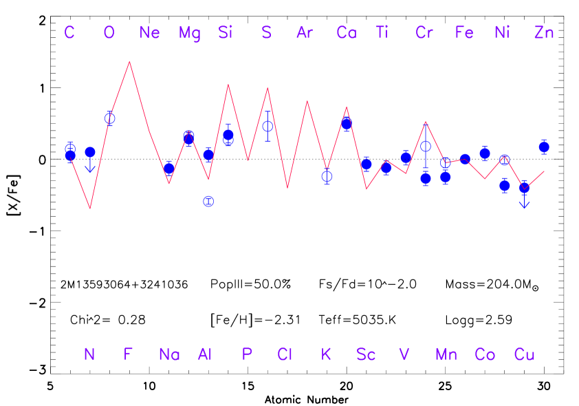
(a) 2M13593064+3241036

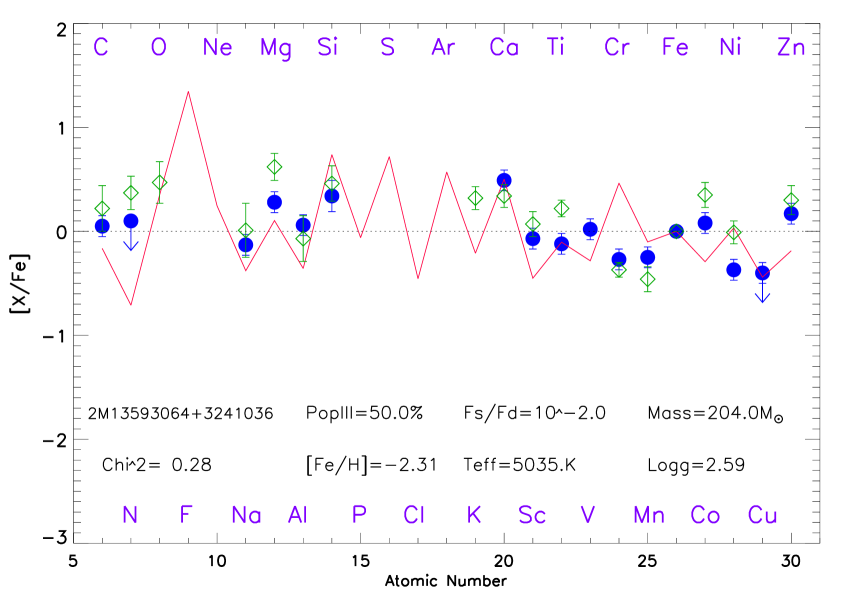
(b) Halo abundance pattern

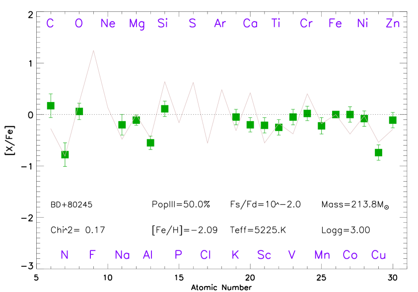
(c) BD+80^∘245

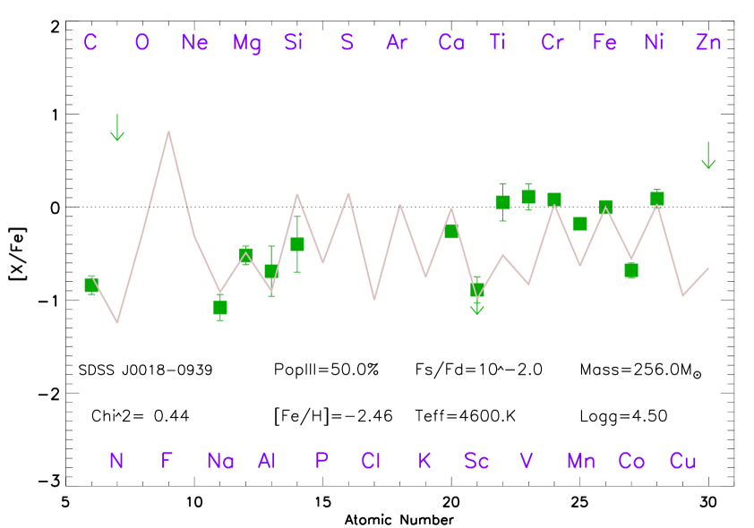
(d) SDSS J0018$-$0939

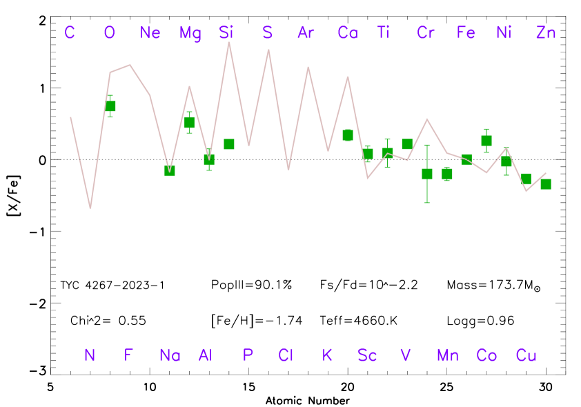
(e) TYC 4267-2023-1

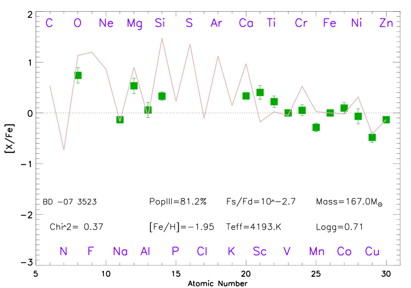
(f) BD $-$07 3523

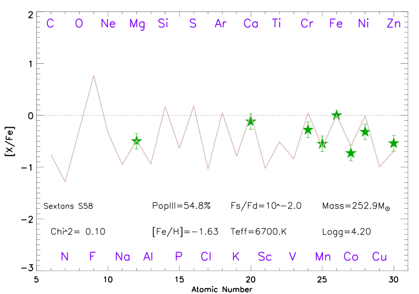
(g) Sextans S58

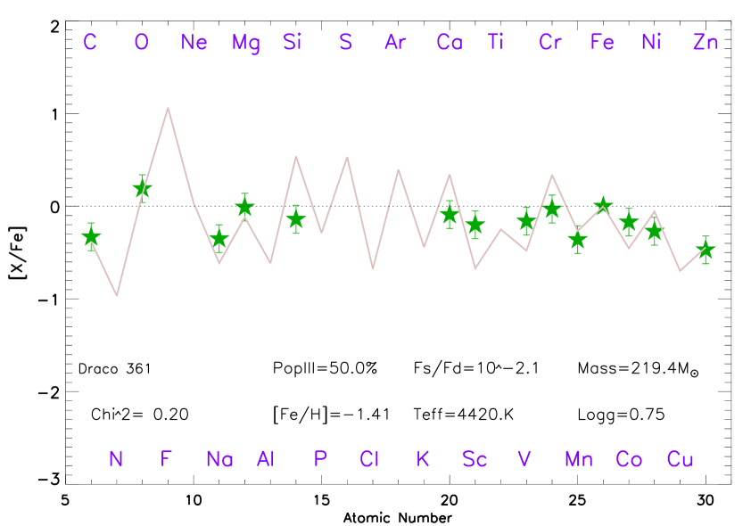
(h) Draco 361

Figure 4: Results of the PISN-explorer analysis. Points are measured chemical abundances while lines are best fits. Listed on the plot are parameters of the fit, along with $T_{\mathrm{eff}}$, $\log g$, and [Fe/H]. Top row: Our new analysis is presented (blue filled circles) and compared to the APOGEE results (a, blue open circles); and the average abundance pattern and the best fit of the Cayrel et al. (2004a) sample (b, green open diamonds). Second row: Previously published candidates for dominant PISN enrichment (green squares), SDSS J0018$-$0939 (c; Aoki et al. 2014) and BD+80^∘245 (d; Salvadori et al. 2019). Third row: Candidates selected from the MINCE survey (e and f; Cescutti et al. 2022). Bottom row: Promising candidates for PISN descendants (green star symbols) in the Sextans (g; Shetrone et al. 2001) and Draco (h; Cohen & Huang 2009) dwarf spheroidal galaxies.

7.1 Our observed candidate: 2M13593064+3241036

In Sec. 4 we reanalysed with FERRE the chemical signature of our PISN candidate. As explained in Sec. 6.2 the fact that 2M13593064+3241036 is more metal-poor than previously published with APOGEE has a direct impact on the analysis and makes the killing ratios [Cu/Fe] and [Zn/Fe] higher than expected, with catastrophic consequences. Additionally, we consider the K measurement as tentative with lower weight in the analysis (see Sec. 6.3). Furthermore, the [Mg/Al] ratio has dramatically increased by $0.69$ dex which clearly attenuates the odd-even effect. Still some key features remain, such as high [Si/Fe] value, and $\rm[Ca/Mg]>0$, but the importance of those is relatively smaller when identifying PISN descendants.

In Fig. 4(a) we show the elemental abundances from Table 6.1 together with the best PISN-explorer fit and parameters. The best fit gives significantly different results than the original analysis: $m_{\text{PISN}}=204.0\,\rm M_{\odot}$ (prev. $193.8\,\rm M_{\odot}$), and $f_{\text{PISN}}=50\%$ (prev. 66%), and $f_{*}/f_{\rm dil}=10^{-2.1}$ (prev. $10^{-2}$). The quality of the fit is now worse (See Fig. 1(a)), in particular the killing element Zn is not anymore well reproduced by the models. Additionally, the odd-even effect is attenuated and the best fit (red line) is unable to reproduce it which is far from we could expect from a PISN descendant. That is consistent with the fact that now the best fit is giving a $f_{\text{PISN}}$ value that is in the limit of the grid, which could be an indication of even lower PISN contribution. Three key results therefore forced us to be cautious on reaching strong conclusions on whether 2M13593064+3241036 is a PISN descendant: (a) the quality of the fit has significantly decreased with the analysis of the higher quality UVES spectrum; (b) the odd-even effect is now clearly reduced; and (c) the high Zn value does not allow us to clearly identify the smoking gun of PISN production. The candidate 2M13593064+3241036 could therefore still be a regular halo star. The following is an additional test we propose to verify this hypothesis.

The authors in Cayrel et al. (2004b) derived precise elemental abundances for 35 very metal-poor halo stars, considered chemically unmixed (Spite et al., 2005). These abundances adequately averaged and NLTE corrected by Andrievsky et al. (2010) can be understood as the mean chemical signature for a regular (C-normal) giant halo star polluted almost exclusively by CCSN. This “representative” abundance pattern is not polluted by PISN at the 99.9% level, and is therefore useful as a comparison sample to test our methodology. Thus, following the methodology described in Sec. 4, we analyzed this average abundance pattern for a regular giant halo star having as result $f_{\rm PISN}=50$%; $f_{*}/f_{\rm dil}=10^{-2.0}$; and $m_{\rm PISN}=231\rm M_{\odot}$. In Fig. 4(b) we show the comparison between 2M13593064+3241036 and the regular giant halo star pattern. As in the case of our candidate we obtained the minimum value of PISN contribution while the mass of the progenitor is slightly higher. In fact, both objects and their best fits seem similar. Main differences are concentrated in lighter elements such us the CNO family where the regular halo star pattern shows smother trend. In addition to it, the odd-even effect is even less clear in 2M13593064+3241036 in the Na-Mg-Al-Si range. Furthermore, the super solar Zn abundance in the regular halo star pattern (as in our APOGEE candidate) is a strong indication of no PISN contribution. The super-solar [Zn/Fe] makes it difficult to establish an unambiguous difference between this star and the average halo star. Therefore we could conclude that 2M13593064+3241036 is likely like other halo stars with no major contribution from PISN pollution.

7.2 Previously reported candidates

In the literature, two stars have been reported as being probable descendants of PISNe: BD+80^∘245 (Salvadori et al., 2019), and SDSS J0018$-$0939 (Aoki et al., 2014). To verify our methods, and compare our approach to their published results, we also analysed these stars with the PISN-explorer, and the result is shown in Figs 4(d) and 4(c).

The star BD+80^∘245 (Carney et al., 1997; Fulbright et al., 2010; Ivans et al., 2003; Roederer et al., 2014), is a low-$\alpha$ halo star (Fig. 4(c)), which was initially proposed as a PISN descendant (Salvadori et al., 2019) based on the low abundance of the killing elements (Cu and Zn). Their originally derived PISN parameters were $f_{\rm PISN}=50$%; $f_{*}/f_{\rm dil}=10^{-4.0}$; and $m_{\rm PISN}=223\rm M_{\odot}$. Our analysis, as explained, is based on the same set of models (Heger & Woosley, 2002; Salvadori et al., 2019) but the way we fit the data with FERRE is different (see Sec. 4). The best solution we get is $f_{\rm PISN}=50$%; $f_{*}/f_{\rm dil}=10^{-2.0}$; and $m_{\rm PISN}=213.8\rm M_{\odot}$ with a $\chi^{2}=0.17$, which is in good agreement with Salvadori et al. (2019). Interestingly, the $f_{*}/f_{\rm dil}$ factor is significantly different in the two analysis while the quality of the fit is similar. The reason for that is that $f_{*}/f_{\rm dil}$ is the least sensitive parameter (see Sec. 2) within the models and the FERRE code tends to go to the limit of the grid.

SDSS J0018$-$0939 is another interesting star that was proposed to be a PISN descendant by Aoki et al. (2014). This star has remarkably low $\alpha$-abundances ($\rm[Mg/Fe]=-0.52$, $\rm[Ca/Fe]=-0.26$), see Fig. 4(d). The authors excluded that the peculiar chemical pattern could not be produced by CCSN or SN Ia. They concluded that the most likely origin is PISN and they attribute a $f_{\rm PISN}=100$% value. Unfortunately, no informative upper limits for Cu and Zn were measured in this star. We used the PISN-explorer to derive PISN parameters from the measured abundances by Aoki et al. (2014) and found $f_{\rm PISN}=50$%; $f_{*}/f_{\rm dil}=10^{-2.0}$; and $m_{\rm PISN}=256\rm M_{\odot}$ with $\chi^{2}=0.44$. Although the $\chi^{2}$ is elevated, we are able to reproduce the chemical signature of lighter elements (See Fig. 4(d)) but the models failed for iron-peak elements. The low $\alpha$ ratios lead to high mass of the progenitor ($256\rm M_{\odot}$) in agreement to what was claimed by Aoki et al. (2014). However, the $f_{\rm PISN}=50$% value suggests that this star could be polluted by PISN but a higher contribution should be attributed to normal Pop II stars exploding as CCSN. Further observations in order to detect and measure killing elements is highly required to confirm the percentage of PISN contamination we see in this star.

The Pristine survey (Starkenburg et al., 2017b) derives metallicities for halo stars based on narrow band filter photometry. In this context, there is also a remarkable observational effort to derive Cu and Zn in metal-poor stars (Caffau et al., 2022). The authors found, among others, three interesting candidates to be polluted by PISN production using also the PISN-explorer. In particular, in their Fig. 12, they show the chemical pattern of TYC 1118-595-1, a very metal-poor star with $\rm[Fe/H]=-2.12$, and derived $f_{\rm PISN}=50$%; $f_{*}/f_{\rm dil}=10^{-2.3}$; and $m_{\rm PISN}=193\rm M_{\odot}$. TYC 2207–992–1 and TYC 1194–507–1 are also reported together with a best fit that suggested that they could be enriched by PISN up to $f_{\rm PISN}=83$% and 90%, respectively. However, the probability of such is significantly smaller than for TYC 1118-595-1 due to the lower quality of the fit. According to what is explained in Sec. 4, we consider that TYC 1118-595-1 is likely reflecting the theoretical predictions in their chemical pattern in a percentage that could be to the order of $f_{\rm PISN}=50$% or slightly smaller. TYC 2207–992–1 is also a very promising candidate with a progenitor mass $m_{\rm PISN}=170\rm M_{\odot}$ while TYC 1194–507–1 has more uncertain origin due to the low quality of the fit.

We also mined the bibliography including high-resolution analysis of halo stars looking for interesting candidates. We found that the vast majority of interesting stars published before 2018 are already included in the JINA database. However, Xing et al. (2019) found an interesting star, J1124+4535, with $\rm[Fe/H]=-1.27$ and $\rm[Zn/Fe]=-0.37$. We also analyzed its chemical signature with the PISN-explorer and found $f_{\rm PISN}=50$%; $f_{*}/f_{\rm dil}=10^{-2.4}$; and $m_{\rm PISN}=231\rm M_{\odot}$. The quality of the fit is relatively good ($\chi^{2}=0.29$) but the absence of Cu measurement or upper limit prevent us to conclude this object is polluted by PISN. We propose to re-observe this interesting object with peculiar chemistry to confirm its origin.

7.3 PISN candidates in classical dwarf galaxies

It is commonly accepted that the classical dwarf spheroidal galaxies are massive enough to retain the chemical products of PISN explosions (see e.g. Bromm & Loeb, 2003; Salvadori et al., 2008). However, their total number of stars is much lower compared to more massive systems. Consequently, the expected fraction of PISN descendants in classical dwarf galaxies is expected to be significantly higher than in the Milky Way. Therefore, classical dwarf galaxies are interesting places to search for PISN descendants. Luckily, within the JINA database there are $\sim 50$ stars from Fornax, Sextans, Draco, and other dwarf satellites. In Figs. 4(g) and 4(h) two interesting examples of the FERRE analysis are shown, Sextans S58 (Shetrone et al., 2001) and Draco 361 (Cohen & Huang, 2009). The quality of both fits are remarkably high with $\chi^{2}=0.10,0.20$, respectively. Additionally, the killing element Zn, is largely subsolar in the atmosphere of the two stars $\rm[Zn/Fe]\sim-0.45$. Actually, the case of Sextans S58 with $f_{\rm PISN}=55$% suggests that the majority of the material this star formed from was polluted mostly by PISN with a mass of $m_{\rm PISN}=253\,\rm M_{\odot}$.

Finally, we also identified another star from JINA database, Draco 3053 (Cohen & Huang, 2009). This star is also Zn-poor with $\rm[Zn/Fe]=-0.3$ and the best set of parameters derived with the PISN-explorer are $f_{\rm PISN}=50$%; $f_{*}/f_{\rm dil}=10^{-2.0}$; and $m_{\rm PISN}=218\rm M_{\odot}$; and $\chi^{2}=0.19$. In this case, the high quality of the fit and the low value of Zn suggest that this star could be indeed polluted by PISN in a percentage close to $f_{\rm PISN}=50$%. Further observations of all of the three candidates in Draco and Sextans galaxies are required.

8 Discussion

In the previous sections we have validated and applied our proposed PISN-explorer methodology to find PISN descendants. Although the 2M13593064+3241036 candidate seems not to be as interesting as expected (mostly due to the initial overestimation of metallicity in APOGEE), its study was useful to understand the capabilities of our methodology. As shown, its chemical signature, and in particular the killing elements Cu and Zn, is not significantly different from that of an average pattern for regular giant halo stars. Indeed, when the contribution of Pop II stars exploding as normal CCSN becomes $>50\%$, the peculiar chemical signatures left by different Pop III star progenitors are essentially lost (Vanni et al. in prep.)

A different situation is presented for BD+80^∘245, shown in Fig. 4(c). For this star we confirm the result provided by Salvadori et al. (2019) and we conclude that it is at least partially (but genuinely) polluted by PISN. The clearly low value of the killing elements that this stars shows is indeed the smoking gun of PISN contamination. On the other hand, the analysis of SDSS J0018$-$0939 shows that while very different from a regular halo star (see Sec. 7.1), the percentage of material produced by PISN may not be as high as originally suggested by Aoki et al. (2014). In any case, some further high-resolution observations of this interesting star are needed to better constrain the amount of Cu and Zn and shed light over the exact amount of material that effectively come from PISN production. At this point we propose using facilities that will be available in the next generation of 30 m telescopes. Moreover, the agreement of our analysis with previous works suggests that the PISN-explorer is efficient in characterising candidates.

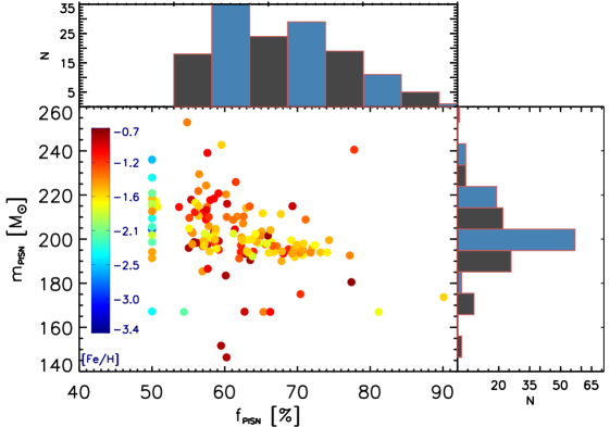
Figure 5: Our catalogue of 166 candidate PISN descendants, shown in the $f_{\rm PISN}-m_{\rm PISN}$ plane, colour-coded by metallicity. Histograms of the candidates are also shown on top and right side panels.

A very challenging issue when identifying the descendants of the very massive first stars is how to discriminate between them and a regular halo star (mostly polluted by Pop II exploding as CCSN). By comparing Fig. 4(b) with 4(c), 4(d), 4(g), and 4(h) it is clear that the chemical signatures that correspond to good fits in this work ($\chi^{2}\lesssim 0.20$) are very different than the mean abundance pattern for a regular giant halo star (Cayrel et al., 2004b). The much higher CNO abundances together with high $\alpha$’s (i.e. Mg, Ti) led to a significantly higher $\chi^{2}$. Obviously, this is deeply related with the fact that the regular halo star pattern is not Zn-poor, which is the most robust indicator. Additionally, as shown in Fig. 4(b), the odd-even effect is clearly lost for atomic numbers higher than Z=19, i.e. for most of the iron-peak elements. According to our novel PISN-explorer, the most efficient way to separate PISN candidates from other halo field stars is a combination of all the criteria presented in Sec. 5, low values of $\chi^{2}$, and the killing elements deficiency $[\rm Cu,Zn/Fe]<0$. In Figs. 4(e) and 4(f) two interesting examples of promising candidates from MINCE survey with subsolar Cu and Zn abundances are shown.

Moreover, the PISN-explorer allowed us to successfully identify very interesting PISN descendants candidates in classical dwarf galaxies (see Fig. 2). Note that none of them are found in the less massive ultra-faint dwarf galaxies. These systems, which are smaller and thus have lower binding energy than classical dSph galaxies, are probably not able to retain the chemical products of energetic PISN (Rossi et al. in prep). Unfortunately, since those from classical dwarfs are typically distant and therefore faint, the next generation of 30 m class telescopes will be required to derive systematically their killing elements.

A final remark concerns the MDF of our 166 selected candidates shown in Fig. 2. It is indeed extremely interesting to see that its main peak is located at $\rm[Fe/H]=-1.7$, i.e. exactly at the level predicted by the cosmological models for the MW formation of de Bennassuti et al. (2017) (see their Fig. 9) and close to the values provided by the parametric study of Salvadori et al. (2019), $\rm[Fe/H]\approx-2$, and by the inhomogeneous chemical enrichment model by Karlsson et al. (2008), $\rm[Fe/H]\approx-2.5$. This result is quite remarkable since the PISN-explorer does not use the iron abundance to select PISN candidates. As explained in Sec. 5, indeed, our selection is solely based on the predicted chemical abundance ratios, [X/Fe]. We should also note that it is very likely that our sample, and thus our selected candidates, are biased towards higher [Fe/H]. In fact, both APOGEE and GALAH rapidly decrease in accuracy in the very metal-poor regime, which is possibly the origin of the second peak at higher [Fe/H]$\approx-1$. Finally, we recall that the iron abundances of PISN descendants is expected to vary in a broad range, $-5<\rm[Fe/H]<0.5$ (see Fig. 7 of Salvadori et al., 2019). Therefore, it is quite normal that in our MDF we find a second and smaller peak at $\rm[Fe/H]=-3.0$. This peak is indeed made by PISN candidates selected from the JINA database, which is naturally biased towards Fe-poor stars.

In Fig. 5 we display the $f_{\rm PISN}-m_{\rm PISN}$ distribution for our 166 selected candidates colour coded by metallicity. While the histograms of $f_{\rm PISN}$ are peaked at lower contribution and monotonically decreases, which is expected, the distribution of $m_{\rm PISN}$ is more condensed around $200\,\rm M_{\odot}$. We also see a more metal-poor population lying at $f_{\rm PISN}=50$%. As explained in Sec. 5 the vast majority of those values should be avoided when selecting candidates. However, as we pointed out, after visual inspection we could consider them as a candidates whether they show a remarkably good fit and Cu and Zn abundances are subsolar. This population was selected following this approach and some of them (due its visibility and/or special features) are included in our golden sample. However, some others are quite faint and we propose to observe at higher SNR when possible with the future high-resolution spectrographs.

9 Conclusions

We have presented a new methodology to identify candidates that have been significantly polluted by PISN in the early Universe. We mined different datasets in order to find chemical patterns that match with what is expected to find if significant PISN production took place. We summarise here the main conclusions of this work:

• Current and upcoming large spectroscopic surveys (APOGEE, GALAH, GES, 4MOST, WEAVE), and existing databases such as JINA, are an invaluable tool to unveil the origin and characteristics of the very massive first stars, which exploded as PISN.

• The PISN-explorer, using the FERRE code in combination with theoretical predictions (Salvadori et al., 2019), is a very efficient methodology when selecting PISN descendant candidates in large databases.

• The MDF of the selected candidates is a confirmation of the predicted peak in PISN production at $\rm[Fe/H]\sim-1.7$ (de Bennassuti et al., 2017).

• killing elements (Cu and Zn), low values of $\alpha$-elements (Mg and Ti), and clear odd-even effect (e.g. high [Mg/Na], and/or high [Mg/Al]), are indicators of PISN production. Therefore, they could be used to efficiently select candidates.

• It is possible that 2M13593064+3241036 was mostly polluted by PISN production but the presence of Zn on its atmosphere does not allow us to confirm this hypothesis. BD+80^∘245 contains significant material that was formed during a PISN event. The $f_{\rm PISN}=$ value previously reported for SDSS J0018$-$0939 (100%) could be significantly lower according to its chemical signature.

• Sextans S58 is the most promising candidate and maybe mostly formed out of PISN material. To confirm this hypothesis further high-resolution follow-up is needed to complete the chemical signature already reported in the literature. Draco 361 and Draco 3053 are also excellent candidates selected from classical dwarf galaxies.

• From our selected 166 candidates we propose 45 of them as a golden catalogue with the most promising and visible stars for future follow-up.

Future high-resolution facilities mounted in the Extremely Large Telescope such as ANDES (Marconi et al., 2022) and other facilities will provide and unbeatable opportunity to observe stars in dwarf satellites, where it is more likely to find PISN descendants. In addition to it, the next generation of large spectroscopic surveys such as WEAVE (Jin et al., in press) and 4MOST (de Jong et al., 2019) with high resolution observations will be an unbeatable place to test the PISN-explorer and finally finding the descendants of the very massive first stars.

10 Data Availability and online material

All the spectroscopic data reduced and analyzed for the present article are fully available under request to the corresponding author. A table with the detected lines in the UVES spectrum of 2M13593064+3241036 is included as online material.

References

- Abdurro’uf et al. (2022) Abdurro’uf et al., 2022, ApJS, 259, 35
- Abel et al. (2002) Abel T., Bryan G. L., Norman M. L., 2002, Science, 295, 93
- Abohalima & Frebel (2018) Abohalima A., Frebel A., 2018, ApJS, 238, 36
- Aguado et al. (2017) Aguado D. S., González Hernández J. I., Allende Prieto C., Rebolo R., 2017, A&A, 605, A40
- Aguado et al. (2021) Aguado D. S., et al., 2021, MNRAS, 500, 889
- Alexeeva et al. (2018) Alexeeva S., Ryabchikova T., Mashonkina L., Hu S., 2018, ApJ, 866, 153
- Allende Prieto et al. (2006) Allende Prieto C., Beers T. C., Wilhelm R., Newberg H. J., Rockosi C. M., Yanny B., Lee Y. S., 2006, ApJ, 636, 804
- Allende Prieto et al. (2014) Allende Prieto C., et al., 2014, A&A, 568, A7
- Allende Prieto et al. (2018) Allende Prieto C., Koesterke L., Hubeny I., Bautista M. A., Barklem P. S., Nahar S. N., 2018, A&A, 618, A25
- Andrievsky et al. (2010) Andrievsky S. M., Spite M., Korotin S. A., Spite F., Bonifacio P., Cayrel R., François P., Hill V., 2010, A&A, 509, A88
- Aoki et al. (2014) Aoki W., Tominaga N., Beers T. C., Honda S., Lee Y. S., 2014, Science, 345, 912
- Asplund et al. (2005) Asplund M., Grevesse N., Sauval A. J., 2005, in Barnes III T. G., Bash F. N., eds, Astronomical Society of the Pacific Conference Series Vol. 336, Cosmic Abundances as Records of Stellar Evolution and Nucleosynthesis. p. 25
- Asplund et al. (2009) Asplund M., Grevesse N., Sauval A. J., Scott P., 2009, ARA&A, 47, 481
- Bergemann et al. (2013) Bergemann M., Kudritzki R.-P., Würl M., Plez B., Davies B., Gazak Z., 2013, ApJ, 764, 115
- Bergemann et al. (2017) Bergemann M., Collet R., Amarsi A. M., Kovalev M., Ruchti G., Magic Z., 2017, ApJ, 847, 15
- Bromm (2013) Bromm V., 2013, Reports on Progress in Physics, 76, 112901
- Bromm & Loeb (2003) Bromm V., Loeb A., 2003, Nature, 425, 812
- Buder et al. (2021) Buder S., et al., 2021, MNRAS, 506, 150
- Caffau et al. (2011) Caffau E., Ludwig H. G., Steffen M., Freytag B., Bonifacio P., 2011, Sol. Phys., 268, 255
- Caffau et al. (2022) Caffau E., et al., 2022, MNRAS,
- Carney et al. (1997) Carney B. W., Wright J. S., Sneden C., Laird J. B., Aguilar L. A., Latham D. W., 1997, AJ, 114, 363
- Cayrel et al. (2004a) Cayrel R., et al., 2004a, A&A, 416, 1117
- Cayrel et al. (2004b) Cayrel R., et al., 2004b, A&A, 416, 1117
- Cescutti et al. (2022) Cescutti G., et al., 2022, arXiv e-prints, p. arXiv:2211.06086
- Cohen & Huang (2009) Cohen J. G., Huang W., 2009, ApJ, 701, 1053
- Cropper et al. (2018) Cropper M., et al., 2018, A&A, 616, A5
- Dalton et al. (2016) Dalton G., et al., 2016, in Evans C. J., Simard L., Takami H., eds, Society of Photo-Optical Instrumentation Engineers (SPIE) Conference Series Vol. 9908, Ground-based and Airborne Instrumentation for Astronomy VI. p. 99081G, doi:10.1117/12.2231078
- De Silva et al. (2015) De Silva G. M., et al., 2015, MNRAS, 449, 2604
- Freudling et al. (2013) Freudling W., Romaniello M., Bramich D. M., Ballester P., Forchi V., García-Dabló C. E., Moehler S., Neeser M. J., 2013, A&A, 559, A96
- Fulbright et al. (2010) Fulbright J. P., et al., 2010, ApJ, 724, L104
- Gaia Collaboration et al. (2021) Gaia Collaboration et al., 2021, A&A, 649, A1
- García Pérez et al. (2016) García Pérez A. E., et al., 2016, AJ, 151, 144
- Gilmore et al. (2012) Gilmore G., et al., 2012, The Messenger, 147, 25
- Gilmore et al. (2022) Gilmore G., et al., 2022, A&A, 666, A120
- Grevesse et al. (2007) Grevesse N., Asplund M., Sauval A. J., 2007, Space Sci. Rev., 130, 105
- Heger & Woosley (2002) Heger A., Woosley S. E., 2002, ApJ, 567, 532
- Hirano et al. (2014) Hirano S., Hosokawa T., Yoshida N., Umeda H., Omukai K., Chiaki G., Yorke H. W., 2014, ApJ, 781, 60
- Hirano et al. (2015) Hirano S., Hosokawa T., Yoshida N., Omukai K., Yorke H. W., 2015, MNRAS, 448, 568
- Hosokawa et al. (2011) Hosokawa T., Omukai K., Yoshida N., Yorke H. W., 2011, Science, 334, 1250
- Ishigaki et al. (2018) Ishigaki M. N., Tominaga N., Kobayashi C., Nomoto K., 2018, The Astrophysical Journal, 857, 46
- Ivans et al. (2003) Ivans I. I., Sneden C., James C. R., Preston G. W., Fulbright J. P., Höflich P. A., Carney B. W., Wheeler J. C., 2003, ApJ, 592, 906
- Karlsson et al. (2008) Karlsson T., Johnson J. L., Bromm V., 2008, ApJ, 679, 6
- Kurucz (2005) Kurucz R. L., 2005, Memorie della Societa Astronomica Italiana Supplementi, 8, 14
- Larson (1998) Larson P. L., 1998, Gaia, 15, 389
- Limongi & Chieffi (2018) Limongi M., Chieffi A., 2018, VizieR Online Data Catalog, p. J/ApJS/237/13
- Lind et al. (2012) Lind K., Bergemann M., Asplund M., 2012, MNRAS, 427, 50
- Lodders et al. (2009) Lodders K., Palme H., Gail H.-P., 2009, Landolt Börnstein,
- Majewski et al. (2017) Majewski S. R., et al., 2017, AJ, 154, 94
- Marconi et al. (2022) Marconi A., et al., 2022, in Evans C. J., Bryant J. J., Motohara K., eds, Society of Photo-Optical Instrumentation Engineers (SPIE) Conference Series Vol. 12184, Ground-based and Airborne Instrumentation for Astronomy IX. p. 1218424, doi:10.1117/12.2628689
- Mashonkina et al. (2007) Mashonkina L., Korn A. J., Przybilla N., 2007, A&A, 461, 261
- Mashonkina et al. (2016) Mashonkina L. I., Sitnova T. N., Pakhomov Y. V., 2016, Astronomy Letters, 42, 606
- McKee & Tan (2008) McKee C. F., Tan J. C., 2008, ApJ, 681, 771
- Mucciarelli et al. (2021) Mucciarelli A., Bellazzini M., Massari D., 2021, A&A, 653, A90
- Nash & Sofer (1990) Nash S. G., Sofer A., 1990, Operations Research Letters, 9, 219
- Nomoto et al. (2013) Nomoto K., Kobayashi C., Tominaga N., 2013, ARA&A, 51, 457
- Nordlander & Lind (2017) Nordlander T., Lind K., 2017, A&A, 607, A75
- Osorio et al. (2020) Osorio Y., Allende Prieto C., Hubeny I., Mészáros S., Shetrone M., 2020, A&A, 637, A80
- Payne (1925) Payne C. H., 1925, PhD thesis, RADCLIFFE COLLEGE.
- Placco et al. (2014) Placco V. M., Frebel A., Beers T. C., Christlieb N., Lee Y. S., Kennedy C. R., Rossi S., Santucci R. M., 2014, ApJ, 781, 40
- Randich et al. (2022) Randich S., et al., 2022, arXiv e-prints, p. arXiv:2206.02901
- Roederer et al. (2014) Roederer I. U., Preston G. W., Thompson I. B., Shectman S. A., Sneden C., Burley G. S., Kelson D. D., 2014, AJ, 147, 136
- Rossi et al. (2021) Rossi M., Salvadori S., Skúladóttir Á., 2021, MNRAS, 503, 6026
- Russell (1941) Russell H. N., 1941, Science, 94, 375
- Salvadori et al. (2008) Salvadori S., Ferrara A., Schneider R., 2008, MNRAS, 386, 348
- Salvadori et al. (2010) Salvadori S., Ferrara A., Schneider R., Scannapieco E., Kawata D., 2010, MNRAS, 401, L5
- Salvadori et al. (2015) Salvadori S., Skúladóttir Á., Tolstoy E., 2015, MNRAS, 454, 1320
- Salvadori et al. (2019) Salvadori S., Bonifacio P., Caffau E., Korotin S., Andreevsky S., Spite M., Skúladóttir Á., 2019, MNRAS, 487, 4261
- Sbordone et al. (2007) Sbordone L., Bonifacio P., Castelli F., 2007, in Kupka F., Roxburgh I., Chan K. L., eds, 2007 International Astronomical Unio Vol. 239, Convection in Astrophysics. pp 71–73, doi:10.1017/S1743921307000142
- Shetrone et al. (2001) Shetrone M. D., Côté P., Sargent W. L. W., 2001, ApJ, 548, 592
- Silk (1977) Silk J., 1977, ApJ, 211, 638
- Spite et al. (2005) Spite M., et al., 2005, A&A, 430, 655
- Starkenburg et al. (2017a) Starkenburg E., Oman K. A., Navarro J. F., Crain R. A., Fattahi A., Frenk C. S., Sawala T., Schaye J., 2017a, MNRAS, 465, 2212
- Starkenburg et al. (2017b) Starkenburg E., et al., 2017b, MNRAS, 471, 2587
- Susa et al. (2014) Susa H., Hasegawa K., Tominaga N., 2014, ApJ, 792, 32
- Takahashi et al. (2018) Takahashi K., Yoshida T., Umeda H., 2018, ApJ, 857, 111
- Tody (1993) Tody D., 1993, in Hanisch R. J., Brissenden R. J. V., Barnes J., eds, Astronomical Society of the Pacific Conference Series Vol. 52, Astronomical Data Analysis Software and Systems II. p. 173
- Tumlinson (2010) Tumlinson J., 2010, ApJ, 708, 1398
- Vrug et al. (2009) Vrug A., ter Braak C., Dicks C., Robinson B., Hyman J., Higdon D., 2009, International Journal of Nonlinear Sciences & Numerical Simulation, 10, 273:290
- Woosley & Weaver (1995) Woosley S. E., Weaver T. A., 1995, ApJS, 101, 181
- Xing et al. (2019) Xing Q.-F., Zhao G., Aoki W., Honda S., Li H.-N., Ishigaki M. N., Matsuno T., 2019, Nature Astronomy, 3, 631
- de Bennassuti et al. (2017) de Bennassuti M., Salvadori S., Schneider R., Valiante R., Omukai K., 2017, MNRAS, 465, 926
- de Jong et al. (2019) de Jong R. S., et al., 2019, The Messenger, 175, 3