Quark-lepton Yukawa ratios and nucleon decay in SU(5) GUTs with type-III seesaw

Abstract

We consider an extension of the Georgi-Glashow SU(5) GUT model by a 45-dimensional scalar and a 24-dimensional fermionic representation, where the latter leads to the generation of the observed light neutrino masses via a combination of a type I and a type III seesaw mechanism. Within this scenario, we investigate the viability of predictions for the ratios between the charged lepton and down-type quark Yukawa couplings, focusing on the second and third family. Such predictions can emerge when the relevant entries of the Yukawa matrices are generated from single joint GUT operators (i.e. under the condition of single operator dominance). We show that three combinations are viable, (i) $y_{\tau}/y_{b}=3/2$, $y_{\mu}/y_{s}=9/2$, (ii) $y_{\tau}/y_{b}=2$, $y_{\mu}/y_{s}=9/2$, and (iii) $y_{\tau}/y_{b}=2$, $y_{\mu}/y_{s}=6$. We extend these possibilities to three toy models, accounting also for the first family masses, and calculate their predictions for various nucleon decay rates. We also analyse how the requirement of gauge coupling unification constrains the masses of potentially light relic states testable at colliders.

1 Introduction

Grand Unified Theories (GUTs) Pati:1973rp ; Pati:1974yy ; Georgi:1974sy ; Georgi:1974yf ; Georgi:1974my ; Fritzsch:1974nn are arguably one of the most appealing extensions of the Standard Model (SM) of particle physics. In 1974, a simple and elegant GUT based on the unifying gauge group SU(5) was proposed by H. Georgi and S. Glashow (GG model) Georgi:1974sy . However, this model is incompatible with the current experimental data for three main reasons. Firstly, the GG model does not allow for gauge coupling unification, which is a necessary condition for a GUT. Secondly, it predicts massless neutrinos, which is in conflict with neutrino oscillation experiments requiring that at least two neutrino should be massive SNO:2002tuh . Thirdly, since the SM Higgs doublet is embedded into a 5-dimensional Higgs representation of SU(5), the GG model predicts the GUT scale relation between the charged lepton and down-type quark Yukawa matrices

$$Y_{e}=Y_{d}^{T}.$$ (1.1)

This relation in particular implies a GUT scale unification of the tau and bottom Yukawa couplings $y_{\tau}=y_{b}$, as well as a unification of the muon and strange Yukawa couplings $y_{\mu}=y_{s}$, which disagrees with the low energy data.

The first shortcoming requires extending the particle content of the minimal model by additional GUT representations and suitably splitting the masses of their component fields such that the running gauge couplings meet. The second shortcoming can be addressed by introducing SU(5) representations that allow neutrino mass generation at the tree level Dorsner:2005fq ; Dorsner:2005ii ; Dorsner:2006hw ; Bajc:2006ia ; Bajc:2007zf ; FileviezPerez:2007bcw ; Dorsner:2006fx or at the loop level FileviezPerez:2016sal ; Kumericki:2017sfc ; Saad:2019vjo ; Dorsner:2019vgf ; Dorsner:2021qwg ; Antusch:2023jok . Finally, the third shortcoming can for instance be resolved by generating the Yukawa couplings from linear combinations of the renormalisable and higher dimensional non-renormalisable operators Ellis:1979fg , or at the renormalizable level by either introducing a 45-dimensional Higgs field and considering linear combinations of couplings between the SM fermions and both the 5- as well as the 45-dimensional Higgs field Dorsner:2006dj , or by introducing vector-like fermions which mix with the SM fermions Babu:2012pb ; Dorsner:2014wva ; FileviezPerez:2018dyf .

However, historically a first and very aesthetic solution for the third problem was proposed by H. Georgi and C. Jarlskog (GJ model) in 1979 Georgi:1979df . In their model, the particle content of the GG model is extended by a 45-dimensional Higgs field (as well as by two 5-dimensional Higgs fields). If the 45-dimensional Higgs field couples to the SM fermions this gives rise to the GUT scale relation

$$Y_{e}=-3Y_{d}^{T}.$$ (1.2)

Considering a linear combination of the operators giving the relations (1.1) and (1.2) would, on the one hand, solve the shortcoming (as already mentioned above), but, on the other hand, predictivity in the Yukawa sector would be lost. Predictivity is however maintained if it is ensured that different generations of charged leptons and down-type quarks couple to different Higgs fields (which can, for example, be achieved when a family symmetry is introduced on top of the gauge symmetry). To achieve predictivity, without referring to any particular family symmetry, the GJ model hypothesizes the following textures of the Yukawa coupling matrices,

$$Y_{d}=\begin{pmatrix}0&&B&&0\\ A&&C&&0\\ 0&&0&&D\end{pmatrix},\quad Y_{e}^{T}=\begin{pmatrix}0&&B&&0\\ A&&-3C&&0\\ 0&&0&&D\end{pmatrix},$$ (1.3)

implying the GUT scale relations $y_{\tau}/y_{b}=1,\,y_{\mu}/y_{s}=-3,\,y_{e}/y_{d}=-1/3$ which were at that time compatible with the experimental data. However, the current data suggests (taking only the known SM particles into account in the renormalization group (RG) evolution) that other ratios such as $y_{\tau}/y_{b}=3/2,\,y_{\mu}/y_{s}=9/2$ are better suited (see e.g. Antusch:2021yqe ).

Interestingly, these latter ratios can be obtained from higher dimensional operators Antusch:2009gu ; Antusch:2013rxa . With these higher dimensional operators at hand, models similar to the GJ model can be build if the following two conditions are satisfied: (i) the Yukawa matrices should be hierarchical, (ii) the 22- and 33- entry should be dominated by a single GUT operator, a concept which is referred to as single operator dominance Antusch:2009gu ; Antusch:2013rxa ; Antusch:2019avd .

Following this approach, non-SUSY GUT scenarios in which neutrino masses are generated by a type I or a type II seesaw have been investigated in Antusch:2021yqe , respectively Antusch:2022afk . For GUT scenarios with a type I seesaw it was shown that the GUT scale ratios $y_{\tau}/y_{b}=3/2$ and $y_{\mu}/y_{s}=9/2$ are compatible with the experimental data. Moreover, for GUT scenarios in which neutrino masses are generated by a type II seesaw it was found, that two combinations of GUT scale relations are viable, namely (i) $y_{\tau}/y_{b}=3/2$ and $y_{\mu}/y_{s}=9/2$ and (ii) $y_{\tau}/y_{b}=2$ and $y_{\mu}/y_{s}=6$.

In this paper we will investigate the viability of such GUT scale ratios for the case that neutrino masses stem from a combination of a type I Minkowski:1977sc ; Yanagida:1979as ; Gell-Mann:1979vob ; Glashow:1979nm ; Mohapatra:1980yp and a type III Foot:1988aq seesaw mechanism. In this regard, we will consider a GUT scenario in which the particle content of the GG model is extended by a fermionic adjoint representation as well as by a 45-dimensional Higgs field. The former representation is needed to generate neutrino masses, while the latter gives rise to operators yielding potentially viable GUT scale Yukawa ratios. Moreover, both of these representations help to allow for gauge coupling unification. Using the Mathematica package ProtonDecay Antusch:2020ztu and extending the above scenario to “toy models” we also compute the nucleon decay widths for various decay channels. Finally, we compute the masses of the added fermion and scalar fields.

The paper is organized as follows: While the GUT scenario as well as the toy models are introduced in Section 2, the procedure for the numerical analysis is explained in Section 3. In Section 4 the results are presented and discussed, before concluding in Section 5. In Appendix A, definitions of the newly introduced Yukawa couplings are given, while all relevant RGEs that we have derived are listed in Appendix B.

2 GUT scenario

2.1 Particle content

The SM fermions are embedded as usual into three generations of ${\bm{\overline{5}_{F}}}_{i}$ and ${\bm{10_{F}}}_{i}$

$${\bm{\overline{5}_{F}}}_{i}= \;d_{i}^{c}(\overline{3},1,\frac{1}{3})\oplus\ell_{i}(1,2,-\frac{1}{2}),$$ (2.4)

$${\bm{10_{F}}}_{i}= \;q_{i}(3,2,\frac{1}{6})\oplus u_{i}^{c}(\overline{3},1,-\frac{2}{3})\oplus e_{i}^{c}(1,1,1).$$ (2.5)

In the considered scenario, neutrino masses are generated via a combination of a type I and a type III seesaw mechanism. The corresponding fermionic singlet $\Sigma_{c}$ and triplet $\Sigma_{b}$ (under $SU(2)_{L}$) are contained in an adjoint fermionic representation

$$\bm{24_{F}}= \;\Sigma_{a}(8,1,0)\oplus\Sigma_{b}(1,3,0)\oplus\Sigma_{c}(1,1,0)\oplus\Sigma_{d}(3,2,-\frac{5}{6})\oplus\Sigma_{e}(\overline{3},2,\frac{5}{6}).$$ (2.6)

Moreover, the GUT Higgs fields decompose under the SM gauge group as

$$\bm{24_{H}}= \;\Phi_{a}(8,1,0)\oplus\Phi_{b}(1,3,0)\oplus\Phi_{c}(1,1,0)\oplus\Phi_{d}(3,2,-\frac{5}{6})\oplus\Phi_{e}(\overline{3},2,\frac{5}{6}),$$ (2.7)

$$\bm{5_{H}}= \;T_{a}(3,1,-\frac{1}{3})\oplus H_{a}(1,2,\frac{1}{2}),$$ (2.8)

$$\bm{45_{H}}= \;\phi_{a}(8,2,\frac{1}{2})\oplus\phi_{b}(6,1,-\frac{1}{3})\oplus\phi_{c}(3,3,-\frac{1}{3})\oplus\phi_{d}(\overline{3},2,-\frac{7}{6})\oplus\phi_{e}(\overline{3},1,-\frac{4}{3})$$

$$\oplus T_{b}(3,1,-\frac{1}{3})\oplus H_{b}(1,2,\frac{1}{2}).$$ (2.9)

After the SU(5) breaking, the color triplets $T_{a}$ and $T_{b}$ mix to yield the mass eigenstates $t_{1}=\cos(\alpha)T_{a}+\sin(\alpha)T_{b}$ and $t_{2}=-\sin(\alpha)T_{a}+\cos(\alpha)T_{b}$. Similarly, $H_{a}$ and $H_{b}$ mix to form the mass eigenstates $h_{1}=\cos(\beta)H_{a}+\sin(\beta)H_{b}$ and $h_{2}^{\perp}=-\sin(\beta)H_{a}+\cos(\beta)H_{b}$, where $h_{1}$ is the SM Higgs doublet.

2.2 Neutrino masses

At tree-level the relevant GUT operators for neutrino mass generation read

$$\mathcal{L}\supset Y_{A}\,\bm{\overline{5}_{F}}\bm{24_{F}}\bm{5_{H}}+Y_{B}\,\bm{\overline{5}_{F}}\bm{24_{F}}\bm{45_{H}}.$$ (2.10)

After the GUT symmetry breaking the following relevant terms emerge

$$\mathcal{L}\supset-Y_{2}\ell\Sigma_{b}H_{a}-Y_{8}\ell\Sigma_{b}H_{b}-Y_{4}\ell\Sigma_{c}H_{a}-Y_{13}\ell\Sigma_{c}H_{b}-m_{\Sigma_{b}}\Sigma_{b}\Sigma_{b}-m_{\Sigma_{c}}\Sigma_{c}\Sigma_{c},$$ (2.11)

where $m_{\Sigma_{b}}$ and $m_{\Sigma_{b}}$ are the respective masses of $\Sigma_{b}$ and $\Sigma_{c}$, and where the GUT scale relations

$$Y_{2}=-\sqrt{\frac{3}{10}}\,Y_{A},\quad Y_{4}=Y_{A},\quad Y_{8}=\frac{\sqrt{5}}{4}\,Y_{B},\quad\text{and}\quad Y_{13}=\frac{\sqrt{3}}{4}\,Y_{B}$$ (2.12)

hold. After the SU(2) triplet $\Sigma_{b}$ and SU(2) singlet $\Sigma_{c}$ have been integrated out and the two Higgs fields $H_{a}$ and $H_{b}$ have taken their vacuum expectation values (vevs) $v_{a}$ and $v_{b}$, where $v_{a}^{2}+v_{b}^{2}=v^{2}=(246\ \text{GeV})^{2}$, and where $v_{a}=v\cos(\beta)$ and $v_{b}=v\sin(\beta)$, the neutrino mass matrix $m_{\nu}$ reads

$$m_{\nu}^{ij}=-\frac{(Y_{2}^{i}\,v_{a}+Y_{8}^{i}\,v_{b})(Y_{2}^{j}\,v_{a}+Y_{8}^{j}\,v_{b})}{4m_{\Sigma_{b}}}-\frac{(Y_{4}^{i}\,v_{a}+Y_{13}^{i}\,v_{b})(Y_{4}^{j}\,v_{a}+Y_{13}^{j}\,v_{b})}{4m_{\Sigma_{c}}}\,.$$ (2.13)

Since the neutrino mass matrix $m_{\nu}$ is of rank two, two massive and one massless neutrino are predicted.

2.3 Quark-lepton Yukawa ratios

With $\bm{X}$ and $\bm{Y}$ representing one or multiple Higgs fields, the charged fermion masses stem from GUT operators of the form

$$\bm{Y_{\overline{5}}}^{ij}\,:\quad{\bm{10_{F}}}_{i}{\bm{\overline{5}_{F}}}_{j}\bm{X}\quad \supset\quad Y_{d}^{ij},\ Y_{e}^{ij}$$ (2.14)

$$\bm{Y_{10}}^{ij}\,:\quad{\bm{10_{F}}}_{i}{\bm{10_{F}}}_{j}\bm{Y}\quad \supset\quad Y_{u}^{ij},$$ (2.15)

where $Y_{u}$, $Y_{d}$ and $Y_{e}$ denote the usual SM charged fermion Yukawa matrices. Assuming in the charged fermion Yukawa sector the concept of single operator dominance, i.e. that each Yukawa entry is dominated by a singlet GUT operator, allows to connect the down-type with the charged lepton Yukawa matrix via group theoretical Clebsch-Gordan (CG) factors $c_{ij}$. In SU(5) GUTs, and considering up to dimension five operators, the potentially viable CG factors are $|c_{ij}|\in\{1/6,\,1/2,\,2/3,\,1,\,3/2,\,2,\,3,\,9/2,\,6,\,9,\,18\}$. The possible GUT operators yielding these ratios are given in Antusch:2009gu ; Antusch:2013rxa . Moreover, if the matrix $\bm{Y_{\overline{5}}}$ is assumed to be of hierarchical nature and dominated by its diagonal entries, then the second and third family down-type quark and charged lepton masses stem dominantly from the GUT operators $\mathcal{O}_{2}$ and $\mathcal{O}_{3}$ dominating the 22 and 33 positions in $\bm{Y_{\overline{5}}}$. Depending on which operators are chosen for $\mathcal{O}_{2}$ and $\mathcal{O}_{3}$, different GUT scale Yukawa ratios $y_{\tau}/y_{b}$ and $y_{\mu}/y_{s}$ are predicted. Our numerical analysis (cf. Section 4) shows that there are only two possible choices for the GUT scale ratio $y_{\tau}/y_{b}$, namely 3/2 or 2. The former CG factor can be complemented by a factor 9/2 for the second family, while for the latter CG factor two different completions, $y_{\mu}/y_{s}=6$ or $y_{\mu}/y_{s}=9/2$, are possible.

2.4 Toy models

We now extend the above motivated scenarios to three toy models which also include the first family. For simplicity, we chose the matrix $\bm{Y_{\overline{5}}}$ to be of diagonal nature. The double ratio $(y_{\mu}y_{d})/(y_{e}y_{s})=10.7^{+1.6}_{-0.9}$, which is nearly constant under renormalization group running (see e.g. Antusch:2013jca ), suggests, that the the ratio $y_{\mu}/y_{s}=9/2$ is best complemented by a ratio $y_{e}/y_{d}=4/9$, while the best completion of the ratio $y_{\mu}/y_{s}=6$ is given by $y_{e}/y_{d}=1/2$. Utilizing these ratios, our three toy models relate the down-type with the charged lepton Yukawa matrix via

$$\text{Model 1:}\quad Y_{e}=\text{diag}\left(\frac{4}{9},\frac{9}{2},\frac{3}{2}\right)\cdot Y_{d}^{T}\,,$$ (2.16)

$$\text{Model 2:}\quad Y_{e}=\text{diag}\left(\frac{4}{9},\frac{9}{2},2\right)\cdot Y_{d}^{T}\,,$$ (2.17)

$$\text{Model 3:}\quad Y_{e}=\text{diag}\left(\frac{1}{2},6,2\right)\cdot Y_{d}^{T}\,.$$ (2.18)

Moreover, for simplicity we assume in each toy model that $\bm{Y_{10}}$ is dominated by the operator $\bm{10_{F}10_{F}5_{H}}$ in all entries, yielding a symmetric up-type Yukawa matrix, i.e. $Y_{u}=Y_{u}^{T}$. Finally, in all toy models neutrino masses stem from a linear combination of the operators $\bm{\overline{5}_{F}24_{F}5_{H}}$ and $\bm{\overline{5}_{F}24_{F}45_{H}}$.

3 Numerical procedure

3.1 Implementation of the charged fermion Yukawa sector

We implement all three toy models at the GUT scale as described in Section 2.4. In all three models the down-type Yukawa matrix $Y_{d}$ is simply implemented as

$$Y_{d}=\text{diag}(y_{1}^{d},y_{2}^{d},y_{3}^{d}),$$ (3.19)

while the charged lepton Yukawa matrix $Y_{e}$ is implemented according to Eq. (2.16), (2.17), and (2.18), respectively. Since $Y_{u}$ is symmetric we use a Takagi decomposition and implement it as

$$Y_{u}=U_{u}^{\dagger}Y_{u}^{\text{diag}}U_{u}^{*},$$ (3.20)

where

$$U_{u}=\begin{pmatrix}1&0&0\\ 0&c_{23}^{u}&s_{23}^{u}\\ 0&-s_{23}^{u}&c_{23}^{u}\end{pmatrix}\begin{pmatrix}c_{13}^{u}&0&s_{13}^{u}e^{-i\delta^{u}}\\ 0&1&0\\ -s_{13}^{u}e^{i\delta^{u}}&0&c_{13}^{u}\end{pmatrix}\begin{pmatrix}c_{12}^{u}&s_{12}^{u}&0\\ -s_{12}^{u}&c_{12}^{u}&0\\ 0&0&1\end{pmatrix}\begin{pmatrix}e^{i\beta_{1}^{u}}&0&0\\ 0&e^{i\beta_{2}^{u}}&0\\ 0&0&1\end{pmatrix},$$ (3.21)

and where $Y_{u}^{\text{diag}}=\text{diag}(y_{1}^{u},y_{2}^{u},y_{3}^{u})$.

3.2 Implementation of the neutrino sector

In order to simplify the analysis we assume in the neutrino sector that the Yukawa matrices $Y_{5}$ and $Y_{6}$ (for the definitions of these couplings, see Appendix A) are of the form

$$Y_{5}=z_{1}\begin{pmatrix}0\\ 1\\ 1\end{pmatrix},\quad\quad Y_{6}=z_{2}\begin{pmatrix}1\\ 1\\ 3\end{pmatrix},$$ (3.22)

where $z_{1}$ and $z_{2}$ are real parameters. Furthermore, we denote the relative phase difference between $m_{\Sigma_{b}}$ and $m_{\Sigma_{c}}$ by $\gamma$ (i.e. $\gamma=\arg(m_{\Sigma_{b}}/m_{\Sigma_{c}})$). This structure is motivated by CSD3 King:2013iva which in the case of type I seesaw has been shown to correctly describe the low-scale neutrino observables together with a normal neutrino mass hierarchy (see e.g. Antusch:2021yqe for a recent work).

3.3 GUT scale parameters and low energy observables

Each toy model contains 33 input parameters which decompose into the GUT scale $M_{\text{GUT}}$, the SU(5) gauge coupling $g_{\text{GUT}}$, the masses of the added particles, $m_{\Phi_{a}}$, $m_{\Phi_{b}}$, $m_{\phi_{a}}$, $m_{\phi_{b}}$, $m_{\phi_{c}}$, $m_{\phi_{d}}$, $m_{\phi_{e}}$, $m_{\Sigma_{a}}$, $m_{\Sigma_{b}}$, $m_{\Sigma_{c}}$, $m_{\Sigma_{d}}$, $m_{t_{1}}$, $m_{t_{2}}$, $m_{h_{2}}$, the singular values $y_{1}^{u}$, $y_{2}^{u}$, $y_{3}^{u}$, $y_{1}^{d}$, $y_{2}^{d}$, $y_{3}^{d}$ and angles $\theta_{12}^{u}$, $\theta_{13}^{u}$, $\theta_{23}^{u}$ as well as phases $\delta^{u}$, $\beta_{1}^{u}$, $\beta_{2}^{u}$ of the charged fermion Yukawa matrices, the parameters of the neutrino Yukawa couplings $z_{1}$, $z_{2}$, and $\gamma$, and the eigenstate mixing angles $\alpha$ and $\beta$. The respective ranges of these input parameters are given by

$$M_{\text{GUT}} <M_{Pl},$$

$$m_{\Phi_{a}},m_{\Phi_{b}},m_{\phi_{a}},m_{\phi_{b}},m_{\phi_{c}},m_{\phi_{d}},m_{\phi_{e}},m_{\Sigma_{a}},m_{\Sigma_{b}},m_{\Sigma_{c}},m_{\Sigma_{d}},m_{h_{2}} \in[1\,\text{TeV},M_{\text{GUT}}],$$

$$m_{t_{1}},m_{t_{2}} \in[10^{11}\,\text{GeV},M_{\text{GUT}}],$$

$$g_{\text{GUT}},\,y_{1}^{u},\,y_{2}^{u},\,y_{3}^{u},\,y_{1}^{d},\,y_{2}^{d},\,y_{3}^{d} \in[0,1],$$ (3.23)

$$\theta_{12}^{u},\,\theta_{13}^{u},\,\theta_{23}^{u},\,\alpha,\,\beta \in[0,\pi/2],$$

$$\delta^{u},\,\beta_{1}^{u},\,\beta_{2}^{u},\,\gamma \in[-\pi,\pi),$$

$$z_{1},\,z_{2} >0.$$

These input parameters are fitted to the 22 low-scale observables (listed in Eq. (3.3)) and the nucleon decay widths of thirteen decay channels (listed in Table I).

$$g_{1},\,g_{2},\,g_{3},$$

$$y_{u},\,y_{c},\,y_{t},\,y_{d},\,y_{s},\,y_{b},\,\theta_{12}^{\text{CKM}},\,\theta_{13}^{\text{CKM}},\,\theta_{23}^{\text{CKM}},\,\delta^{\text{CKM}},\,y_{e},\,y_{\mu},\,y_{\tau},\,\hskip 17.07182pt$$ (3.24)

$$\Delta m_{21}^{2},\,\Delta m_{31}^{2},\,\theta_{12}^{\text{PMNS}},\,\theta_{13}^{\text{PMNS}},\,\theta_{23}^{\text{PMNS}},\,\delta^{\text{PMNS}}.$$

For the SM gauge couplings and Yukawa observables we take the experimental values from Antusch:2013jca , while the values for the neutrino sector are taken from NuFIT 5.1 Esteban:2020cvm .

	decay channel	$\tau/\mathcal{B}$ [year]	$\Gamma_{\text{partial}}$ [GeV]	Reference
Proton:	$p\rightarrow\pi^{0}\,e^{+}$	$>\,2.4\cdot 10^{34}$	$<\,8.7\cdot 10^{-67}$	Super-Kamiokande:2020wjk
	$p\rightarrow\pi^{0}\,\mu^{+}$	$>\,1.6\cdot 10^{34}$	$<\,1.3\cdot 10^{-66}$	Super-Kamiokande:2020wjk
	$p\rightarrow\eta^{0}\,e^{+}$	$>\,1.0\cdot 10^{34}$	$<\,2.0\cdot 10^{-66}$	Super-Kamiokande:2017gev
	$p\rightarrow\eta^{0}\,\mu^{+}$	$>\,4.7\cdot 10^{33}$	$<\,4.4\cdot 10^{-66}$	Super-Kamiokande:2017gev
	$p\rightarrow K^{0}\,e^{+}$	$>\,1.1\cdot 10^{33}$	$<\,1.9\cdot 10^{-65}$	Brock:2012ogj
	$p\rightarrow K^{0}\,\mu^{+}$	$>\,3.6\cdot 10^{33}$	$<\,5.8\cdot 10^{-66}$	Super-Kamiokande:2022egr
	$p\rightarrow\pi^{+}\,\overline{\nu}$	$>\,3.9\cdot 10^{32}$	$<\,5.3\cdot 10^{-65}$	Super-Kamiokande:2013rwg
	$p\rightarrow K^{+}\,\overline{\nu}$	$>\,6.6\cdot 10^{33}$	$<\,3.2\cdot 10^{-66}$	Takhistov:2016eqm
Neutron:	$n\rightarrow\pi^{-}\,e^{+}$	$>\,5.3\cdot 10^{33}$	$<\,3.9\cdot 10^{-66}$	Super-Kamiokande:2017gev
	$n\rightarrow\pi^{-}\,\mu^{+}$	$>\,3.5\cdot 10^{33}$	$<\,5.9\cdot 10^{-66}$	Super-Kamiokande:2017gev
	$n\rightarrow\pi^{0}\,\overline{\nu}$	$>\,1.1\cdot 10^{33}$	$<\,1.9\cdot 10^{-65}$	Super-Kamiokande:2013rwg
	$n\rightarrow\eta^{0}\,\overline{\nu}$	$>\,5.6\cdot 10^{32}$	$<\,3.7\cdot 10^{-65}$	Brock:2012ogj
	$n\rightarrow K^{0}\,\overline{\nu}$	$>\,1.2\cdot 10^{32}$	$<\,1.7\cdot 10^{-64}$	Brock:2012ogj

Table I: Current experimental bounds on the decay widths $\Gamma_{\text{partial}}$, respectively lifetime $\tau/\mathcal{B}$ at 90 % confidence level, where $\mathcal{B}$ is the branching ratio for the decay channel. See also Dev:2022jbf for future projections and sensitivities of various upcoming detectors.

3.4 Fitting procedure

After implementing the input parameters given in Eq. (3.3) at the GUT scale we compute the RG evolution to the $Z$ scale. For the gauge couplings we use a 2-loop running, while we compute the running of the Yukawa matrices and the effective neutrino mass operator at 1-loop. The nucleon decay widths are computed using the Mathematica package Proton Decay Antusch:2020ztu (for a description of the calculation see e.g. Antusch:2021yqe ). Taking into account all observables we compute at the low scale the $\chi^{2}$-function which we minimize using a differential evolution algorithm giving us a benchmark point. With a flat prior distribution we calculate $4\times 10^{6}$ data points performing a Markov-chain-Monte-Carlo (MCMC) analysis using an adaptive Metropolis-Hastings algorithm Metropolis-Hastings-algorithm which we start from this benchmark point. These data points are finally used to compute the highest posterior density (HPD) ranges of various quantities.

4 Results

The results of our numerical analysis are presented in this section. We are in particular interested in the nucleon decay predictions, the intermediate-scale particle masses as well as the low scale predictions for the charged lepton and down-type quark mass ratios. In Section 4.1 we show the results of our minimization procedure. Starting an MCMC analysis from these benchmark points allows us to obtain the HPD ranges of various quantities. The results of this analysis is presented in Section 4.2.

4.1 Benchmark points

We obtain for all three models benchmark points through a minimization of the $\chi^{2}$-function as described in Section 3. In Table II the input parameters for the respective benchmark points are listed. Moreover, the dominant pulls $\chi_{i}^{2}$ are presented in Table III. All three models can be very well fitted to the data. The strongest (though quite small) pull is given by the first and second family down-type quark masses. The biggest difference between the three models is the respectively favored GUT scale. For Models 2 and 3 a GUT scale above $10^{17}$ GeV is favored, while for the benchmark point of Model 1 a GUT scale below $10^{16}$ GeV is obtained. This also results in different results for the predicted nucleon decay rates (cf. Section 4.2). Another difference is the preferred choice of some of the intermediate-scale particle masses. In the presented benchmark point the mass of the fermionic field $\Sigma_{a}$ is obtained to be at the GUT scale for Model 1, at the intermediate scale for Model 2 and at the relatively low scale (23 TeV) for Model 3. Moreover, a mass of the leptoquark $\phi_{c}$ of 1 TeV, respectively 4 TeV is obtained for Model 3, respectively Model 2, whereas for Model 1 the mass of this field is above $10^{6}$ TeV. For the HPD results of these particle masses confer the subsequent section.

		Model 1			Model 2			Model 3
$g_{\text{GUT}}\;/\;10^{-1}$		5.94			6.17			6.33
$\log_{10}(M_{\text{GUT}}\;/\;\text{GeV})$		15.6			17.2			17.3
$\log_{10}(m_{\phi_{a}}\;/\;\text{GeV})$		9.43			14.0			16.7
$\log_{10}(m_{\phi_{c}}\;/\;\text{GeV})$		9.02			3.63			3.00
$\log_{10}(m_{\Sigma_{a}}\;/\;\text{GeV})$		15.6			7.53			4.36
$\log_{10}(m_{\Sigma_{b}}\;/\;\text{GeV})$		14.2			14.9			14.7
$\log_{10}(m_{\Sigma_{c}}\;/\;\text{GeV})$		13.8			12.8			13.2
$\log_{10}(m_{\Sigma_{d}}\;/\;\text{GeV})$		14.2			15.9			14.1
$y_{1}^{u}\;/\;10^{-6}$		2.63			2.11			1.99
$y_{2}^{u}\;/\;10^{-3}$		1.46			1.37			1.18
$y_{3}^{u}\;/\;10^{-1}$		4.54			4.26			3.65
$y_{1}^{d}\;/\;10^{-6}$		6.21			6.30			5.46
$y_{2}^{d}\;/\;10^{-4}$		1.31			1.21			0.99
$y_{3}^{d}\;/\;10^{-3}$		6.64			6.01			5.36
$z_{1}\;/\;10^{-1}$		3.50			9.42			6.86
$z_{2}\;/\;10^{-1}$		1.12			0.32			0.50
$\gamma$		1.85			1.48			1.68
$\alpha$		0.50			1.00			0.50

Table II: The GUT scale input parameters of the benchmark points for all three models.

	$\chi^{2}$	$\chi^{2}_{y_{d}}$	$\chi^{2}_{y_{s}}$	$\chi^{2}_{y_{b}}$	$\chi^{2}_{y_{\mu}}$	$\chi^{2}_{y_{\tau}}$	$\chi^{2}_{\Gamma({p\rightarrow\pi^{0}e^{+}})}$
Model 1	1.36	0.27	0.41	0.06	0.04	0.14	0.44
Model 2	0.31	0.23	0.02	0.01	0.00	0.05	0.00
Model 3	0.33	0.17	0.03	0.00	0.06	0.07	0.00

Table III: The total $\chi^{2}$ as well as the dominant pulls $\chi_{i}^{2}$ for the benchmark points of all three models.

4.2 Highest posterior densities

As described in Section 3.4 we vary the input parameters listed in Eq. 3.3 around their benchmark points (cf. Table II) using an MCMC analysis. From these generated points we then compute the HPD intervals of various parameters and observables.

In Figures 1 – 4 we use the following color coding: For Model 1, 2, and 3 the HPD intervals of various quantities are colored red, green, and blue, respectively, while the 1$\sigma$ (2$\sigma$) HPD intervals are colored dark (light).

4.2.1 Quark-lepton mass ratios

The HPD results for the low scale charged lepton and down-type quark mass ratios are presented in Figure 1. The horizontal dashed line represents the current experimental central value, whereas the white region shows the current experimental 1$\sigma$ range. Clearly, all three models are capable of reproducing viable mass ratios. This strengthens the results of the benchmark points in the previous subsection (cf. Tables II and III). Compared to Model 2 and 3, Model 1 gives a bit smaller predictions for the mass ratios for all three generations.

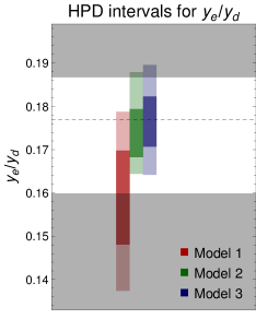
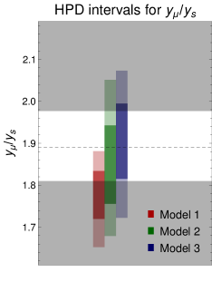
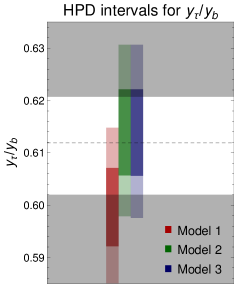
Figure 1: Low scale ($M_{Z}$) HPD intervals for charged lepton and down-type quark Yukawa ratios of all three families. The 1$\sigma$ (2$\sigma$) HDP intervals are colored dark (light).

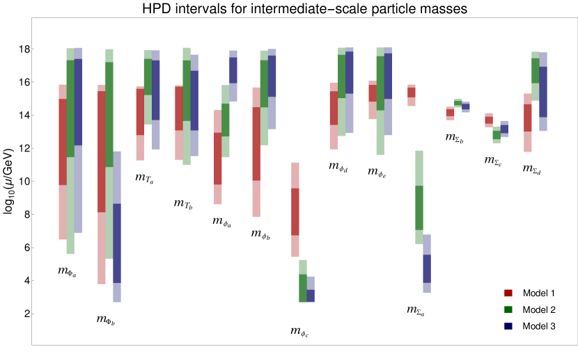
Figure 2: HPD intervals of the intermediate-scale particle masses. The 1$\sigma$ (2$\sigma$) HDP intervals are colored dark (light).

4.2.2 Intermediate-scale particle masses

Figure 2 shows the predicted HPD intervals of the intermediate-scale particle masses. Most of the masses are predicted to be out of the reach of current and future colliders, because they would either produce too much proton decay, spoil gauge coupling unification or because of the fit of the fermion masses. But interestingly, the fields $\Phi_{b}$, $\phi_{c}$ and $\Sigma_{a}$ are not only potentially within the reach of future searches, but can also be used to distinguish between the different models: An observation of the one of the fields $\Phi_{b}$ or $\Sigma_{a}$ would strongly hint towards Model 3, while an observation of the field $\phi_{c}$ would disfavor Model 1. In fact, the most promising lookout could be for the leptoquark $\phi_{c}$. The upper bound of the HPD 1$\sigma$ range is predicted to be 23 TeV (2.8 TeV) in Model 2 (3), whereas the upper bound of the 2$\sigma$ intervals is 175 TeV (17 TeV). In the following, we briefly state the current collider bounds on these particles.

The scalar triplet, $\Phi_{b}$, with zero hypercharge, residing in the $\bm{24_{H}}$ multiplet is expected to be light in Model 3. Note that $\Phi_{b}$ contains a neutral $\Phi_{b}^{0}$ and a pair of singly charged $\Phi_{b}^{\pm}$ states. In the low-energy effective theory, a term of the form $h_{1}^{\dagger}\Phi_{b}^{2}h_{1}$ is allowed, where $h_{1}$ is the SM Higgs doublet. As a result of this coupling, the SM Higgs can decay into two photons $h^{0}\to\gamma\gamma$ via a one-loop diagram mediated by the $\Phi_{b}^{\pm}$ states. Consistency with the LHC data requires these charged states to have masses above 250 GeV Chabab:2018ert .

The scalar leptoquark $\phi_{c}$, which is a triplet of SU(2)_L, resides around the TeV scale in Models 2 and 3. In both models, its coupling to the SM fermions is dominated by the third-generation quark and lepton. Hence, within our scenarios, its decay branching fraction is dominated by a $b\tau$ final state. Since leptoquarks carry color, they are efficiently produced at the LHC through gluon-initiated as well as quark-initiated processes Diaz:2017lit . LHC searches of $pp\to b\overline{b}\tau\overline{\tau}$ from pair-produced leptoquarks rule out leptoquark masses below 1400 GeV ATLAS:2019qpq ; ATLAS:2021oiz .

As can be seen from Eq. (A.26), the color octet fermion $\Sigma_{a}$, which is expected to be light in Model 3, couples, for example, to a singlet down-quark (lepton doublet) and a super-heavy colored triplet (octet) scalar. Consequently, the lifetime of a TeV scale $\Sigma_{a}$ is expected to be large, and it behaves like a long-lived gluino that typically arises in split-supersymmetric scenarios Giudice:2004tc ; Arkani-Hamed:2004zhs . Long-lived colored particles would hadronize, forming so-called R-hadrons Farrar:1978xj . These bound states are comprised of the long-lived state and light SM quarks or gluons, and interact with the detector material, typically inside the calorimeters, via hadronic interactions of the light-quark constituents. Motivated by split-supersymmetric models, R-hadrons are extensively searched for at the LHC ATLAS:2019gqq ; CMS:2020iwv . Non-observation of any deviations of the signal from the expected background puts to a lower limit on the mass of the long-lived $\Sigma_{a}$ fermion of 2000 GeV ATLAS:2019gqq .

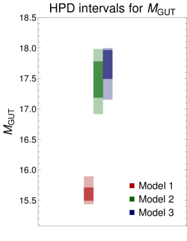
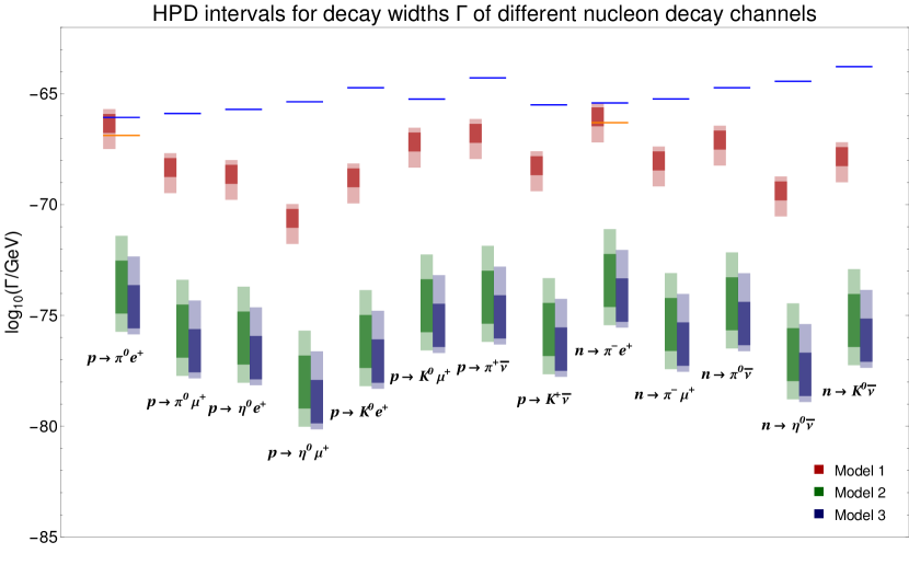
Figure 3: Predicted HPD intervals of the GUT scale. The 1$\sigma$ (2$\sigma$) HDP intervals are colored dark (light).

Figure 4: Predicted HPD intervals of the nucleon decay widths. The 1$\sigma$ (2$\sigma$) HDP intervals are colored dark (light). For each decay channel the blue line segments represent the current experimental constraints. The future Hyper-Kamiokande constraints for the decay channels $p\rightarrow\pi^{0}e^{+}$ and $n\rightarrow\pi^{-}e^{+}$ are indicated by orange line segments.

4.2.3 Nucleon decay width and GUT scale

Figure 4 shows the predictions for the HPD intervals of the GUT scale $M_{\text{GUT}}$. Moreover, the predicted HPD ranges for the nucleon decay widths of the various decay channels are presented in Figure 4. The blue line segments in the latter picture indicate the current experimental bounds at 90 % confidence level (cf. Table I). Moreover, the future constraints on the decay widths for the decay channels $p\rightarrow\pi^{0}e^{+}$ and $n\rightarrow\pi^{-}e^{+}$ which will be provided by Hyper-Kamiokande Hyper-Kamiokande:2018ofw are presented by orange line segments.

In Figure 4 it can be seen that Model 1 clearly predicts the GUT scale to be below $10^{16}$ GeV. On the other hand, a much larger GUT scale is preferred by the Models 2 and 3. Since the nucleon decay width is inversely proportional to the forth power of the GUT scale in the case of gauge boson mediated nucleon decay, this also results in strongly different prediction for the nucleon decay widths of the various channels as it can be seen in Figure 4. The nucleon decay predictions for Model 1 are very close to the current bounds, the 1$\sigma$ HPD interval of the proton decay channel $p\rightarrow\pi^{0}e^{+}$ will be fully probed by Hyper-Kamiokande. Moreover, Hyper-Kamiokande will probe most of the 1$\sigma$ HPD interval of the neutron decay channel $n\rightarrow\pi^{-}e^{+}$. On the other hand, the gauge boson mediated nucleon decay is highly suppressed in Models 2 and 3 and cannot be probed by any planed experiments. Therefore, observation of nucleon decay in the decay channels $p\rightarrow\pi^{0}e^{+}$ and $n\rightarrow\pi^{-}e^{+}$ would clearly favour Model 1 over the Models 2 and 3.

5 Conclusion

In this paper we considered an extension of the Georgi-Glashow SU(5) GUT scenario by a 45-dimensional scalar and a 24-dimensional fermionic representation. Neutrino masses in this scenario are generated by a combination of a type I and a type III seesaw mechanism. Assuming the concept of single operator dominance we investigated which GUT scale charged lepton and down-type quark Yukawa ratios can be viable for the second and third family and found that three combinations work: (i) $y_{\tau}/y_{b}=3/2$, $y_{\mu}/y_{s}=9/2$, (ii) $y_{\tau}/y_{b}=2$, $y_{\mu}/y_{s}=9/2$, and (iii) $y_{\tau}/y_{b}=2$, $y_{\mu}/y_{s}=6$. Also taking into account the origin of the first family masses we extended these possibilities to three toy models and analyzed various of their predictions. We showed that experimental discrimination between these models could be possible since they predict different nucleon decay rates as well as distinct light relics.

Appendix A Definition of new Yukawa couplings

The Lagrangian density contains the two terms

$$\mathcal{L}\supset Y_{A}\,\bm{\overline{5}_{F}}^{i}\bm{24_{F}5_{H}}+Y_{B}\,\bm{\overline{5}_{F}}^{i}\bm{24_{F}45_{H}}.$$ (A.25)

After the GUT symmetry breaking they decompose into

$$\mathcal{L}=\; \sqrt{\frac{2}{15}}Y_{A}\,d^{c}\Sigma_{c}T_{a}-\sqrt{\frac{3}{10}}Y_{A}\,\ell\Sigma_{c}H_{a}+Y_{A}\,d^{c}\Sigma_{a}T_{a}+Y_{A}\,\ell\Sigma_{b}H_{a}+$$

$$Y_{A}\,d^{c}\Sigma_{d}H_{a}+Y_{A}\,\ell\Sigma_{e}T_{a}+\sqrt{\frac{5}{12}}Y_{B}\,d^{c}\Sigma_{c}T_{b}+\frac{\sqrt{5}}{4}Y_{B}\,\ell\Sigma_{c}H_{b}+$$

$$\frac{1}{2\sqrt{2}}Y_{B}\,d^{c}\Sigma_{a}T_{b}+\frac{1}{\sqrt{2}}Y_{B}\,d^{c}\Sigma_{a}\phi_{b}+\frac{1}{\sqrt{2}}Y_{B}\,\ell\Sigma_{a}\phi_{a}+\frac{1}{\sqrt{2}}Y_{B}\,d^{c}\Sigma_{b}\phi_{c}+$$

$$\frac{\sqrt{3}}{4}Y_{B}\,\ell\Sigma_{b}H_{b}-\frac{1}{\sqrt{2}}Y_{B}\,d^{c}\Sigma_{d}\phi_{a}-\frac{1}{2\sqrt{6}}Y_{B}\,d^{c}\Sigma_{d}H_{b}+\frac{1}{\sqrt{2}}Y_{B}\,\ell\Sigma_{d}\phi_{e}-$$

$$\frac{1}{\sqrt{2}}Y_{B}\,d^{c}\Sigma_{e}\phi_{d}+\frac{1}{2\sqrt{2}}Y_{B}\,\ell\Sigma_{e}T_{b}-\frac{1}{\sqrt{2}}Y_{B}\,\ell\Sigma_{e}\phi_{c}\,$$

$$\equiv\; Y_{1}\,d^{c}\Sigma_{c}T_{a}+Y_{2}\,\ell\Sigma_{c}H_{a}+Y_{3}\,d^{c}\Sigma_{a}T_{a}+Y_{4}\,\ell\Sigma_{b}H_{a}+$$

$$Y_{5}\,d^{c}\Sigma_{d}H_{a}+Y_{6}\,\ell\Sigma_{e}T_{a}+Y_{7}\,d^{c}\Sigma_{c}T_{b}+Y_{8}\,\ell\Sigma_{c}H_{b}+$$

$$Y_{9}\,d^{c}\Sigma_{a}T_{b}+Y_{10}\,d^{c}\Sigma_{a}\phi_{b}+Y_{11}\,\ell\Sigma_{a}\phi_{a}+Y_{12}\,d^{c}\Sigma_{b}\phi_{c}+$$

$$Y_{13}\,\ell\Sigma_{b}H_{b}+Y_{14}\,d^{c}\Sigma_{d}\phi_{a}+Y_{15}\,d^{c}\Sigma_{d}H_{b}+Y_{16}\,\ell\Sigma_{d}\phi_{e}+$$

$$Y_{17}\,d^{c}\Sigma_{e}\phi_{d}+Y_{18}\,\ell\Sigma_{e}T_{b}+Y_{19}\,\ell\Sigma_{e}\phi_{c}\;,$$ (A.26)

where we defined the Yukawa matrices $Y_{N}$, with $N=1,\dots,19$.

Appendix B Renormalization group equations

Here the RGEs for the gauge and Yukawa couplings as well as for the effective neutrino mass operator are listed. We have used the Mathematica package SARAH Staub:2008uz ; Staub:2013tta to obtain the RGEs for the gauge and Yukawa couplings. The SM contribution for the RGE of the effective neutrino mass operator is taken from Antusch:2001ck . In order to compute the new contribution for this RGE we have used the method described therein. We use the following definition for the Heaviside-Theta function

$$\mathcal{H}(\mu,m)=\begin{cases}1,\;\;\textrm{for}\;\mu\geq m,\\ 0,\;\;\textrm{for}\;\mu<m.\end{cases}$$ (B.27)

B.1 Gauge couplings

The RGEs for gauge couplings ($i,k=1-3$) are given by

$$\mu\frac{dg_{i}}{d\mu}=\frac{\beta^{g_{i}}_{1-\text{loop}}}{16\pi^{2}}+\frac{\beta^{g_{i}}_{2-\text{loop}}}{(16\pi^{2})^{2}}\,,$$ (B.28)

where $\beta^{g_{i}}_{1-\text{loop}}$ is the 1-loop and $\beta^{g_{i}}_{2-\text{loop}}$ is the 2-loop contribution given by

$$\beta^{g_{i}}_{1-\text{loop}}=\bigg{\{}a_{i}^{\text{SM}}+\mathcal{H}(\mu,m)\Delta a_{i}\bigg{\}}g_{i}^{3}\,$$ (B.29)

$$\beta^{g_{i}}_{2-\text{loop}}=\sum_{k}b^{\text{SM}}_{ik}g^{2}_{k}+\sum_{k}\Delta b_{ik}g^{2}_{k}\;\mathcal{H}(\mu,m)+\beta^{Y,\text{SM}}_{i}+\Delta\beta^{Y}_{i}.$$ (B.30)

Here, $a_{i}^{\text{SM}}$, $b^{SM}_{ik}$ and $\beta^{Y,\text{SM}}_{i}$ are the well known SM 1-loop and 2-loop coefficients as well as Yukawa contributions Cheng:1973nv ; Machacek:1983fi . Moreover, the $\Delta\beta^{Y}_{i}$ are given by

$$\Delta\beta^{Y}_{i}=g_{i}^{3}\sum_{k}c_{ik}Y^{T}_{k}Y^{\ast}_{k}\;\mathcal{H}^{2}_{k},$$ (B.31)

where we introduced the abbreviation $\mathcal{H}^{2}_{k}=\mathcal{H}(\mu,m_{F})\mathcal{H}(\mu,m_{H})$ associated to each of the Yukawa interactions, where, $F$ and $H$ refer to the BSM fermion and scalar appearing in that interaction, respectively, and where the $c_{ik}$ are given by

$$c_{1k}=-\bigg{\{}\frac{1}{5},\frac{3}{10},\frac{8}{15},\frac{9}{20},\frac{29}{10},\frac{17}{5},\frac{1}{5},\frac{3}{10},\frac{8}{15},\frac{8}{15},\frac{12}{5},\frac{3}{5},\frac{9}{20},\frac{116}{15},\frac{29}{10},\frac{17}{5},\frac{29}{5},\frac{17}{5},\frac{51}{10}\bigg{\}},$$ (B.32)

$$c_{2k}=-\bigg{\{}0,\frac{1}{2},0,\frac{11}{4},\frac{3}{2},3,0,\frac{1}{2},0,0,4,6,\frac{11}{4},4,\frac{3}{2},3,3,3,\frac{9}{2}\bigg{\}},$$ (B.33)

$$c_{3k}=-\bigg{\{}\frac{1}{2},0,\frac{13}{3},0,2,1,\frac{1}{2},0,\frac{13}{3},\frac{13}{3},6,\frac{3}{2},0,\frac{16}{3},2,1,4,1,\frac{3}{2}\bigg{\}}.$$ (B.34)

Finally, the $\Delta a_{i}$ and $\Delta b_{i}$ are given as a sum over the 1-loop and 2-loop coefficients of the BSM fermions and scalars, i.e.

$$\Delta a_{i}=\sum_{I}\Delta a_{i}^{I}\,,\qquad\Delta b_{i}=\sum_{I}\Delta b_{i}^{I}\,,$$ (B.35)

where $I$ runs over all BSM particles. The 1-loop coefficients are then given by

$$\Delta a_{i}^{\phi_{a}}=\left\{\frac{4}{5},\frac{4}{3},2\right\},\quad\Delta a_{i}^{\phi_{b}}=\left\{\frac{2}{15},0,\frac{5}{6}\right\},\quad\Delta a_{i}^{\phi_{c}}=\left\{\frac{1}{5},2,\frac{1}{2}\right\},$$

$$\Delta a_{i}^{\phi_{d}}=\left\{\frac{49}{30},\frac{1}{2},\frac{1}{3}\right\},\quad\Delta a_{i}^{\phi_{e}}=\left\{\frac{16}{15},0,\frac{1}{6}\right\},\quad\Delta a_{i}^{\Phi_{a}}=\{0,0,\frac{1}{2}\},$$

$$\Delta a_{i}^{\Phi_{b}}=\left\{0,\frac{1}{3},0\right\},\quad\Delta a_{i}^{\Sigma_{a}}=\{0,0,2\},\quad\Delta a_{i}^{\Sigma_{b}}=\left\{0,\frac{4}{3},0\right\},$$

$$\Delta a_{i}^{\Sigma_{d,e}}=\left\{\frac{5}{3},1,\frac{2}{3}\right\},\quad\Delta a_{i}^{h^{\perp}}=\left\{\frac{1}{10},\frac{1}{6},0\right\},\quad\Delta a_{i}^{t,t^{\perp}}=\left\{\frac{1}{15},0,\frac{1}{6}\right\},$$ (B.36)

whereas the 2-loop coefficients read

$$\Delta b_{ik}^{\phi_{a}}=\left(\begin{array}[]{ccc}\frac{36}{25}&\frac{36}{5}&\frac{144}{5}\\ \frac{12}{5}&\frac{52}{3}&48\\ \frac{18}{5}&18&84\\ \end{array}\right),\quad\Delta b_{ik}^{\phi_{b}}=\left(\begin{array}[]{ccc}\frac{8}{75}&0&\frac{16}{3}\\ 0&0&0\\ \frac{2}{3}&0&\frac{115}{3}\\ \end{array}\right),\quad\Delta b_{ik}^{\phi_{c}}=\left(\begin{array}[]{ccc}\frac{4}{25}&\frac{24}{5}&\frac{16}{5}\\ \frac{8}{5}&56&32\\ \frac{2}{5}&12&11\\ \end{array}\right),$$ (B.46)

$$\Delta b_{ik}^{\phi_{d}}=\left(\begin{array}[]{ccc}\frac{2401}{150}&\frac{147}{10}&\frac{392}{15}\\ \frac{49}{10}&\frac{13}{2}&8\\ \frac{49}{15}&3&\frac{22}{3}\\ \end{array}\right),\quad\Delta b_{ik}^{\phi_{e}}=\left(\begin{array}[]{ccc}\frac{1024}{75}&0&\frac{256}{15}\\ 0&0&0\\ \frac{32}{15}&0&\frac{11}{3}\\ \end{array}\right),\quad\Delta b_{ik}^{\Phi_{a}}=\left(\begin{array}[]{ccc}0&0&0\\ 0&0&0\\ 0&0&21\\ \end{array}\right),$$ (B.56)

$$\Delta b_{ik}^{\Phi_{b}}=\left(\begin{array}[]{ccc}0&0&0\\ 0&\frac{28}{3}&0\\ 0&0&0\\ \end{array}\right),\quad\Delta b_{ik}^{\Sigma_{a}}=\left(\begin{array}[]{ccc}0&0&0\\ 0&0&0\\ 0&0&48\\ \end{array}\right),\quad\Delta b_{ik}^{\Sigma_{b}}=\left(\begin{array}[]{ccc}0&0&0\\ 0&\frac{64}{3}&0\\ 0&0&0\\ \end{array}\right),$$ (B.66)

$$\Delta b_{ik}^{\Sigma_{d,e}}=\left(\begin{array}[]{ccc}\frac{25}{12}&\frac{15}{4}&\frac{20}{3}\\ \frac{5}{4}&\frac{49}{4}&4\\ \frac{5}{6}&\frac{3}{2}&\frac{38}{3}\\ \end{array}\right),\quad\Delta b_{ik}^{h^{\perp}}=\left(\begin{array}[]{ccc}\frac{9}{50}&\frac{9}{10}&0\\ \frac{3}{10}&\frac{13}{6}&0\\ 0&0&0\\ \end{array}\right),\quad\Delta b_{ik}^{t,t^{\perp}}=\left(\begin{array}[]{ccc}\frac{4}{75}&0&\frac{16}{15}\\ 0&0&0\\ \frac{2}{15}&0&\frac{11}{3}\\ \end{array}\right).$$ (B.76)

B.2 Yukawa matrices

The RGEs of the Yukawa matrices read

$$\mu\frac{dY_{f}}{d\mu}=\frac{\beta_{f}}{16\pi^{2}},$$ (B.77)

where $f=\{u,d,e,k\}$ and $(k=1,\dots,19)$. For the SM Yukawa matrices $Y_{u}$, $Y_{d}$ and $Y_{e}$ (i.e. $f={u,d,e}$) the beta functions are given by

$$\beta_{f}=\beta_{f}^{\text{SM}}+\delta\beta_{f},$$ (B.78)

where $\beta_{f}^{\text{SM}}$ is the SM beta function Cheng:1973nv ; Machacek:1983fi , and where

$$\delta\beta_{f}=Y_{f}T_{1}+\sum_{k}a^{f}_{k}(Y_{k})_{j}(Y^{T}_{d}Y^{\ast}_{k})_{i}\;\mathcal{H}^{2}_{k}\,.$$ (B.79)

Here, we have defined $T_{1}$ as

$$T_{1}=Y^{T}_{2}Y^{\ast}_{2}\;\mathcal{H}^{2}_{2}+\frac{3}{2}Y^{T}_{4}Y^{\ast}_{4}\;\mathcal{H}^{2}_{4}+3Y^{T}_{5}Y^{\ast}_{5}\;\mathcal{H}^{2}_{5}.$$ (B.80)

while the $a_{k}^{f}$ are given by

$$a_{k}^{u}=\Big{\{}0,0,0,0,0,0,0,0,0,0,0,0,0,0,0,0,0,0,0\Big{\}},$$ (B.81)

$$a_{k}^{d}=\left\{\frac{1}{2},0,\frac{4}{3},0,3,0,\frac{1}{2},0,\frac{4}{3},\frac{4}{3},0,\frac{3}{2},0,\frac{8}{3},1,0,2,0,0\right\},$$ (B.82)

$$a_{k}^{e}=\left\{0,-\frac{3}{2},0,\frac{15}{4},0,\frac{3}{2},0,\frac{1}{2},0,0,4,0,\frac{3}{4},0,0,\frac{3}{2},0,\frac{3}{2},\frac{9}{4}\right\}.$$ (B.83)

In order to simplify the notation, from hereon, associated to each Yukawa $Y_{i}\to Y_{i}\;\mathcal{H}^{2}_{i}$ must be understood. The beta function of the Yukawa matrices $Y_{1},\dots,Y_{19}$ then read

$$\beta_{1}= \;Y_{1}\left(-\frac{1}{5}g^{2}_{1}-4g^{2}_{3}+\sum_{k}a_{k}^{1}Y^{T}_{k}Y^{\ast}_{k}\right)+\left(Y_{d}Y^{\dagger}_{d}\right)Y_{1}+\sum_{w}b_{w}^{1}\left(Y^{T}_{1}Y^{\ast}_{w}\right)Y_{w}$$

$$+\frac{8}{3}\left(Y^{T}_{3}Y^{\ast}_{9}\right)Y_{7}+2\left(Y^{T}_{6}Y^{\ast}_{18}\right)Y_{7},$$ (B.84)

$$\beta_{2}= \;Y_{2}\left(-\frac{9}{20}g^{2}_{1}-\frac{9}{4}g^{2}_{2}+\sum_{k}a_{k}^{2}Y^{T}_{k}Y^{\ast}_{k}+T\right)+\left(-\frac{3}{2}Y_{e}^{T}Y^{\ast}_{e}\right)Y_{2}+\sum_{w}b_{w}^{2}\left(Y^{T}_{2}Y^{\ast}_{w}\right)Y_{w}$$

$$+\frac{3}{2}\left(Y^{T}_{4}Y^{\ast}_{13}\right)Y_{8}+3\left(Y^{T}_{5}Y^{\ast}_{15}\right)Y_{8},$$ (B.85)

$$\beta_{3}= \;Y_{3}\left(-\frac{1}{5}g^{2}_{1}-13g^{2}_{3}+\sum_{k}a_{k}^{3}Y^{T}_{k}Y^{\ast}_{k}\right)+\left(Y_{d}Y^{\dagger}_{d}\right)Y_{3}+\sum_{w}b_{w}^{3}\left(Y^{T}_{3}Y^{\ast}_{w}\right)Y_{w}$$

$$+\left(Y^{T}_{1}Y^{\ast}_{7}\right)Y_{9}+2\left(Y^{T}_{6}Y^{\ast}_{18}\right)Y_{9},$$ (B.86)

$$\beta_{4}= \;Y_{4}\left(-\frac{9}{20}g^{2}_{1}-\frac{33}{4}g^{2}_{2}+\sum_{k}a_{k}^{4}Y^{T}_{k}Y^{\ast}_{k}+T\right)+\left(\frac{5}{2}Y_{e}^{T}Y^{\ast}_{e}\right)Y_{4}+\sum_{w}b_{w}^{4}\left(Y^{T}_{4}Y^{\ast}_{w}\right)Y_{w}$$

$$+\left(Y^{T}_{2}Y^{\ast}_{8}\right)Y_{13}+3\left(Y^{T}_{5}Y^{\ast}_{15}\right)Y_{13},$$ (B.87)

$$\beta_{5}= \;Y_{5}\left(-\frac{29}{20}g^{2}_{1}-\frac{9}{4}g^{2}_{2}-8g^{2}_{3}+\sum_{k}a_{k}^{5}Y^{T}_{k}Y^{\ast}_{k}+T\right)+\left(3Y_{d}Y^{\dagger}_{d}\right)Y_{5}+\sum_{w}b_{w}^{5}\left(Y^{T}_{5}Y^{\ast}_{w}\right)Y_{w}$$

$$+\left(Y^{T}_{2}Y^{\ast}_{8}\right)Y_{15}+\frac{3}{2}\left(Y^{T}_{4}Y^{\ast}_{13}\right)Y_{15},$$ (B.88)

$$\beta_{6}= \;Y_{6}\left(-\frac{17}{10}g^{2}_{1}-\frac{9}{2}g^{2}_{2}-4g^{2}_{3}+\sum_{k}a_{k}^{6}Y^{T}_{k}Y^{\ast}_{k}\right)+\left(\frac{1}{2}Y^{T}_{e}Y^{\ast}_{e}\right)Y_{6}+\sum_{w}b_{w}^{6}\left(Y^{T}_{6}Y^{\ast}_{w}\right)Y_{w}$$

$$+\left(Y^{T}_{1}Y^{\ast}_{7}\right)Y_{18}+\frac{8}{3}\left(Y^{T}_{3}Y^{\ast}_{9}\right)Y_{18},$$ (B.89)

$$\beta_{7}= \;Y_{7}\left(-\frac{1}{5}g^{2}_{1}-4g^{2}_{3}+\sum_{k}a_{k}^{7}Y^{T}_{k}Y^{\ast}_{k}\right)+\left(Y_{d}Y^{\dagger}_{d}\right)Y_{7}+\sum_{w}b_{w}^{7}\left(Y^{T}_{7}Y^{\ast}_{w}\right)Y_{w}$$

$$+\left(2Y^{T}_{18}Y^{\ast}_{6}\right)Y_{1}+\frac{8}{3}\left(Y^{T}_{9}Y^{\ast}_{3}\right)Y_{1},$$ (B.90)

$$\beta_{8}= \;Y_{8}\left(-\frac{9}{20}g^{2}_{1}-\frac{9}{4}g^{2}_{2}+\sum_{k}a_{k}^{8}Y^{T}_{k}Y^{\ast}_{k}\right)+\left(Y_{e}^{T}Y^{\ast}_{e}\right)Y_{8}+\sum_{w}b_{w}^{8}\left(Y^{T}_{8}Y^{\ast}_{w}\right)Y_{w}$$

$$+\frac{3}{2}\left(Y^{T}_{13}Y^{\ast}_{4}\right)Y_{2}+3\left(Y^{T}_{15}Y^{\ast}_{5}\right)Y_{2},$$ (B.91)

$$\beta_{9}= \;Y_{9}\left(-\frac{1}{5}g^{2}_{1}-13g^{2}_{3}+\sum_{k}a_{k}^{9}Y^{T}_{k}Y^{\ast}_{k}\right)+\left(Y_{d}Y^{\dagger}_{d}\right)Y_{9}+\sum_{w}b_{w}^{9}\left(Y^{T}_{9}Y^{\ast}_{w}\right)Y_{w}$$

$$+2\left(Y^{T}_{18}Y^{\ast}_{6}\right)Y_{3}+\left(Y^{T}_{7}Y^{\ast}_{1}\right)Y_{3},$$ (B.92)

$$\beta_{10}= \;Y_{10}\left(-\frac{1}{5}g^{2}_{1}-13g^{2}_{3}+\sum_{k}a_{k}^{10}Y^{T}_{k_{10}}Y^{\ast}_{k}\right)+\left(Y_{d}Y^{\dagger}_{d}\right)Y_{10}+\sum_{w}b_{w}^{10}\left(Y^{T}_{10}Y^{\ast}_{w}\right)Y_{w},$$ (B.93)

$$\beta_{11}= \;Y_{11}\left(-\frac{9}{20}g^{2}_{1}-\frac{9}{4}g^{2}_{2}-9g^{2}_{3}+\sum_{k}a_{k}^{11}Y^{T}_{k}Y^{\ast}_{k}\right)+\left(Y_{e}^{T}Y^{\ast}_{e}\right)Y_{11}+\sum_{w}b_{w}^{11}\left(Y^{T}_{11}Y^{\ast}_{w}\right)Y_{w},$$ (B.94)

$$\beta_{12}= \;Y_{12}\left(-\frac{1}{5}g^{2}_{1}-6g^{2}_{2}-4g^{2}_{3}+\sum_{k}a_{k}^{12}Y^{T}_{k}Y^{\ast}_{k}\right)+\left(Y_{d}Y^{\dagger}_{d}\right)Y_{12}+\sum_{w}b_{w}^{12}\left(Y^{T}_{12}Y^{\ast}_{w}\right)Y_{w},$$ (B.95)

$$\beta_{13}= \;Y_{13}\left(-\frac{9}{20}g^{2}_{1}-\frac{33}{4}g^{2}_{2}+\sum_{k}a_{k}^{13}Y^{T}_{k}Y^{\ast}_{k}\right)+\left(\frac{1}{2}Y_{e}^{T}Y^{\ast}_{e}\right)Y_{13}+\sum_{w}b_{w}^{13}\left(Y^{T}_{13}Y^{\ast}_{w}\right)Y_{w}$$

$$+3\left(Y^{T}_{15}Y^{\ast}_{5}\right)Y_{4}+\left(Y^{T}_{8}Y^{\ast}_{2}\right)Y_{4},$$ (B.96)

$$\beta_{14}= \;Y_{14}\left(-\frac{29}{20}g^{2}_{1}-\frac{9}{4}g^{2}_{2}-8g^{2}_{3}+\sum_{k}a_{k}^{14}Y^{T}_{k}Y^{\ast}_{k}\right)+\left(Y_{d}Y^{\dagger}_{d}\right)Y_{14}+\sum_{w}b_{w}^{14}\left(Y^{T}_{14}Y^{\ast}_{w}\right)Y_{w},$$ (B.97)

$$\beta_{15}= \;Y_{15}\left(-\frac{29}{20}g^{2}_{1}-\frac{9}{4}g^{2}_{2}-8g^{2}_{3}+\sum_{k}a_{k}^{15}Y^{T}_{k}Y^{\ast}_{k}\right)+\left(Y_{d}Y^{\dagger}_{d}\right)Y_{15}+\sum_{w}b_{w}^{15}\left(Y^{T}_{15}Y^{\ast}_{w}\right)Y_{w}$$

$$+\frac{3}{2}\left(Y^{T}_{13}Y^{\ast}_{4}\right)Y_{5}+\left(Y^{T}_{8}Y^{\ast}_{2}\right)Y_{5},$$ (B.98)

$$\beta_{16}= \;Y_{16}\left(-\frac{17}{10}g^{2}_{1}-\frac{9}{2}g^{2}_{2}-4g^{2}_{3}+\sum_{k}a_{k}^{16}Y^{T}_{k}Y^{\ast}_{k}\right)+\left(\frac{1}{2}Y_{e}^{T}Y^{\ast}_{e}\right)Y_{16}+\sum_{w}b_{w}^{16}\left(Y^{T}_{16}Y^{\ast}_{w}\right)Y_{w},$$ (B.99)

$$\beta_{17}= \;Y_{17}\left(-\frac{29}{20}g^{2}_{1}-\frac{9}{4}g^{2}_{2}-8g^{2}_{3}+\sum_{k}a_{k}^{17}Y^{T}_{k}Y^{\ast}_{k}\right)+\left(Y_{d}Y^{\dagger}_{d}\right)Y_{17}+\sum_{w}b_{w}^{17}\left(Y^{T}_{17}Y^{\ast}_{w}\right)Y_{w},$$ (B.100)

$$\beta_{18}= \;Y_{18}\left(-\frac{17}{10}g^{2}_{1}-\frac{9}{2}g^{2}_{2}-4g^{2}_{3}+\sum_{k}a_{k}^{18}Y^{T}_{k}Y^{\ast}_{k}\right)+\left(\frac{1}{2}Y_{e}^{T}Y^{\ast}_{e}\right)Y_{18}+\sum_{w}b_{w}^{18}\left(Y^{T}_{18}Y^{\ast}_{w}\right)Y_{w}$$

$$+\left(Y^{T}_{7}Y^{\ast}_{1}\right)Y_{6}+\frac{8}{3}\left(Y^{T}_{9}Y^{\ast}_{3}\right)Y_{6},$$ (B.101)

$$\beta_{19}= \;Y_{19}\left(-\frac{17}{20}g^{2}_{1}-\frac{9}{2}g^{2}_{2}-4g^{2}_{3}+\sum_{k}a_{k}^{19}Y^{T}_{k}Y^{\ast}_{k}\right)+\left(\frac{1}{2}Y_{e}^{T}Y^{\ast}_{e}\right)Y_{19}+\sum_{w}b_{w}^{19}\left(Y^{T}_{19}Y^{\ast}_{w}\right)Y_{w},$$ (B.102)

where the coefficients $a_{k}^{f}$ are given by

$$a_{k}^{1}=\{3,1,\frac{8}{3},0,0,2,\frac{3}{2},1,0,0,0,0,0,0,0,0,0,0,0\},$$ (B.103)

$$a_{k}^{2}=\{\frac{3}{2},\frac{5}{2},0,\frac{3}{2},3,0,\frac{3}{2},1,0,0,0,0,0,0,0,0,0,0,0\},$$ (B.104)

$$a_{k}^{3}=\{1,0,\frac{9}{2},0,0,2,0,0,\frac{1}{2},\frac{1}{2},1,0,0,0,0,0,0,0,0\},$$ (B.105)

$$a_{k}^{4}=\{0,1,0,\frac{11}{4},3,0,0,0,0,0,0,\frac{3}{2},\frac{1}{2},0,0,0,0,0,0\},$$ (B.106)

$$a_{k}^{5}=\{0,1,0,\frac{3}{2},\frac{9}{2},0,0,0,0,0,0,0,0,\frac{4}{3},\frac{1}{2},\frac{1}{2},0,0,0\},$$ (B.107)

$$a_{k}^{6}=\{1,0,\frac{8}{3},0,0,4,0,0,0,0,0,0,0,0,0,0,1,\frac{1}{2},\frac{3}{4}\},$$ (B.108)

$$a_{k}^{7}=\{\frac{3}{2},1,0,0,0,0,3,1,\frac{8}{3},0,0,0,0,0,0,0,0,2,0\},$$ (B.109)

$$a_{k}^{8}=\{\frac{3}{2},1,0,0,0,0,\frac{3}{2},\frac{5}{2},0,0,0,0,\frac{3}{2},0,3,0,0,0,0\},$$ (B.110)

$$a_{k}^{9}=\{0,0,\frac{1}{2},0,0,0,1,0,\frac{9}{2},\frac{1}{2},1,0,0,0,0,0,0,2,0\},$$ (B.111)

$$a_{k}^{10}=\{0,0,\frac{1}{2},0,0,0,0,0,\frac{1}{2},\frac{19}{6},1,0,0,0,0,0,0,0,0\},$$ (B.112)

$$a_{k}^{11}=\{0,0,\frac{1}{2},0,0,0,0,0,\frac{1}{2},\frac{1}{2},6,0,0,1,0,0,0,0,0\},$$ (B.113)

$$a_{k}^{12}=\{0,0,0,\frac{1}{2},0,0,0,0,0,0,0,4,\frac{1}{2},0,0,0,0,0,1\},$$ (B.114)

$$a_{k}^{13}=\{0,0,0,\frac{1}{2},0,0,0,1,0,0,0,\frac{3}{2},\frac{11}{4},0,3,0,0,0,0\},$$ (B.115)

$$a_{k}^{14}=\{0,0,0,0,\frac{1}{2},0,0,0,0,0,1,0,0,5,\frac{1}{2},\frac{1}{2},0,0,0\},$$ (B.116)

$$a_{k}^{15}=\{0,0,0,0,\frac{1}{2},0,0,1,0,0,0,0,\frac{3}{2},\frac{4}{3},\frac{9}{2},\frac{1}{2},0,0,0\},$$ (B.117)

$$a_{k}^{16}=\{0,0,0,0,\frac{1}{2},0,0,0,0,0,0,0,0,\frac{4}{3},\frac{1}{2},4,0,0,0\},$$ (B.118)

$$a_{k}^{17}=\{0,0,0,0,0,\frac{1}{2},0,0,0,0,0,0,0,0,0,0,5,\frac{1}{2},\frac{3}{4}\},$$ (B.119)

$$a_{k}^{18}=\{0,0,0,0,0,\frac{1}{2},1,0,\frac{8}{3},0,0,0,0,0,0,0,1,4,\frac{3}{4}\},$$ (B.120)

$$a_{k}^{19}=\{0,0,0,0,0,\frac{1}{2},0,0,0,0,0,1,0,0,0,0,1,\frac{1}{2},4\},$$ (B.121)

while the coefficients $b_{k}^{f}$ read

$$b_{w}^{1}=\{0,0,\frac{4}{3},0,1,0,\frac{3}{2},0,0,\frac{4}{3},0,\frac{3}{2},0,\frac{8}{3},1,0,2,0,0\},$$ (B.122)

$$b_{w}^{2}=\{0,0,0,\frac{3}{4},0,\frac{3}{2},0,\frac{3}{2},0,0,4,0,\frac{3}{4},0,0,\frac{3}{2},0,\frac{3}{2},\frac{9}{4}\},$$ (B.123)

$$b_{w}^{3}=\{\frac{1}{2},0,0,0,1,0,\frac{1}{2},0,0,\frac{4}{3},0,\frac{3}{2},0,\frac{8}{3},1,0,2,0\},$$ (B.124)

$$b_{w}^{4}=\{0,\frac{1}{2},0,0,0,\frac{3}{2},0,\frac{1}{2},0,0,4,0,\frac{9}{4},0,0,\frac{3}{2},0,\frac{3}{2},\frac{9}{4}\},$$ (B.125)

$$b_{w}^{5}=\{\frac{1}{2},0,\frac{4}{3},0,0,0,\frac{1}{2},0,\frac{4}{3},\frac{4}{3},0,\frac{3}{2},0,\frac{8}{3},4,0,2,0,0\},$$ (B.126)

$$b_{w}^{6}=\{0,\frac{1}{2},0,\frac{3}{4},0,0,0,\frac{1}{2},0,0,4,0,\frac{3}{4},0,0,\frac{3}{2},0,\frac{7}{2},\frac{9}{4}\},$$ (B.127)

$$b_{w}^{7}=\{\frac{3}{2},0,\frac{4}{3},0,1,0,0,0,\frac{4}{3},\frac{4}{3},0,\frac{3}{2},0,\frac{8}{3},1,0,2,0,0\},$$ (B.128)

$$b_{w}^{8}=\{0,\frac{3}{2},0,\frac{3}{4},0,\frac{3}{2},0,0,0,0,4,0,\frac{3}{4},0,0,\frac{3}{2},0,\frac{3}{2},\frac{9}{4}\},$$ (B.129)

$$b_{w}^{9}=\{\frac{1}{2},0,4,0,1,0,\frac{1}{2},0,0,\frac{4}{3},0,\frac{3}{2},0,\frac{8}{3},1,0,2,0,0\},$$ (B.130)

$$b_{w}^{10}=\{\frac{1}{2},0,\frac{4}{3},0,1,0,\frac{1}{2},0,\frac{4}{3},0,0,\frac{3}{2},0,\frac{8}{3},1,0,2,0,0\},$$ (B.131)

$$b_{w}^{11}=\{0,\frac{1}{2},0,\frac{3}{4},0,\frac{3}{2},0,\frac{1}{2},0,0,0,0,\frac{3}{4},0,0,\frac{3}{2},0,\frac{3}{2},\frac{9}{4}\},$$ (B.132)

$$b_{w}^{12}=\{\frac{1}{2},0,\frac{4}{3},0,1,0,\frac{1}{2},0,\frac{4}{3},\frac{4}{3},0,0,0,\frac{8}{3},1,0,2,0,0\},$$ (B.133)

$$b_{w}^{13}=\{0,\frac{1}{2},0,\frac{9}{4},0,\frac{3}{2},0,\frac{1}{2},0,0,4,0,0,0,0,\frac{3}{2},0,\frac{3}{2},\frac{9}{4}\},$$ (B.134)

$$b_{w}^{14}=\{\frac{1}{2},0,\frac{4}{3},0,1,0,\frac{1}{2},0,\frac{4}{3},\frac{4}{3},0,\frac{3}{2},0,0,1,0,2,0,0\},$$ (B.135)

$$b_{w}^{15}=\{\frac{1}{2},0,\frac{4}{3},0,4,0,\frac{1}{2},0,\frac{4}{3},\frac{4}{3},0,\frac{3}{2},0,\frac{8}{3},0,0,2,0,0\},$$ (B.136)

$$b_{w}^{16}=\{0,\frac{1}{2},0,\frac{3}{4},0,\frac{3}{2},0,\frac{1}{2},0,0,4,0,\frac{3}{4},0,0,0,0,\frac{3}{2},\frac{9}{4}\},$$ (B.137)

$$b_{w}^{17}=\{\frac{1}{2},0,\frac{4}{3},0,1,0,\frac{1}{2},0,\frac{4}{3},\frac{4}{3},0,\frac{3}{2},0,\frac{8}{3},1,0,0,0,0\},$$ (B.138)

$$b_{w}^{18}=\{0,\frac{1}{2},0,\frac{3}{4},0,\frac{7}{2},0,\frac{1}{2},0,0,4,0,\frac{3}{4},0,0,\frac{3}{2},0,0,\frac{9}{4}\},$$ (B.139)

$$b_{w}^{19}=\{0,\frac{1}{2},0,\frac{3}{4},0,\frac{3}{2},0,\frac{1}{2},0,0,4,0,\frac{3}{4},0,0,\frac{3}{2},0,\frac{3}{2},0\}.$$ (B.140)

B.3 Effective neutrino mass operator

The RGE for the effective neutrino mass operator reads

$$16\pi^{2}\mu\frac{d\kappa}{d\mu}= \;\beta_{\kappa}^{\text{SM}}+\Delta\beta_{\kappa},$$ (B.141)

where $\beta_{\kappa}^{\text{SM}}$ is the SM contribution as given in Antusch:2001ck and $\Delta\beta_{\kappa}$ is the correction due to the added BSM particles. For $\Delta\beta_{\kappa}$ we find

$$\Delta\beta_{\kappa}=\kappa\bigg{(} \frac{1}{2}Y_{2}^{*}Y_{2}^{T}+\frac{3}{4}Y_{4}^{*}Y_{4}^{T}+\frac{3}{2}Y_{6}^{*}Y_{6}^{T}+\frac{1}{2}Y_{8}^{*}Y_{8}^{T}+4Y_{11}^{*}Y_{11}^{T}+\frac{3}{4}Y_{13}^{*}Y_{13}^{T}+\frac{3}{2}Y_{16}^{*}Y_{16}^{T}$$

$$+ \;\frac{3}{2}Y_{18}^{*}Y_{18}^{T}+\frac{9}{4}Y_{19}^{*}Y_{19}^{T}\bigg{)}+\bigg{(}\frac{1}{2}Y_{2}^{*}Y_{2}^{T}+\frac{3}{4}Y_{4}^{*}Y_{4}^{T}+\frac{3}{2}Y_{6}^{*}Y_{6}^{T}+\frac{1}{2}Y_{8}^{*}Y_{8}^{T}$$

$$+ \;4Y_{11}^{*}Y_{11}^{T}+\frac{3}{4}Y_{13}^{*}Y_{13}^{T}+\frac{3}{2}Y_{16}^{*}Y_{16}^{T}+\frac{3}{2}Y_{18}^{*}Y_{18}^{T}+\frac{9}{4}Y_{19}^{*}Y_{19}^{T}\bigg{)}^{T}\kappa$$

$$+ \;\bigg{(}2Y_{2}^{T}Y_{2}^{*}+3Y_{4}^{T}Y_{4}^{*}+6Y_{5}^{T}Y_{5}^{*}+2Y_{8}^{T}Y_{8}^{*}+3Y_{13}^{T}Y_{13}^{*}+6Y_{15}^{T}Y_{15}^{*}\bigg{)}\kappa\;.$$ (B.142)

References

- (1) J. C. Pati and A. Salam, “Is Baryon Number Conserved?,” Phys. Rev. Lett. 31 (1973) 661–664.
- (2) J. C. Pati and A. Salam, “Lepton Number as the Fourth Color,” Phys. Rev. D 10 (1974) 275–289. [Erratum: Phys.Rev.D 11, 703–703 (1975)].
- (3) H. Georgi and S. L. Glashow, “Unity of All Elementary Particle Forces,” Phys. Rev. Lett. 32 (1974) 438–441.
- (4) H. Georgi, H. R. Quinn, and S. Weinberg, “Hierarchy of Interactions in Unified Gauge Theories,” Phys. Rev. Lett. 33 (1974) 451–454.
- (5) H. Georgi, “The State of the Art—Gauge Theories,” AIP Conf. Proc. 23 (1975) 575–582.
- (6) H. Fritzsch and P. Minkowski, “Unified Interactions of Leptons and Hadrons,” Annals Phys. 93 (1975) 193–266.
- (7) SNO Collaboration, Q. R. Ahmad et al., “Direct evidence for neutrino flavor transformation from neutral current interactions in the Sudbury Neutrino Observatory,” Phys. Rev. Lett. 89 (2002) 011301, arXiv:nucl-ex/0204008.
- (8) I. Dorsner and P. Fileviez Perez, “Unification without supersymmetry: Neutrino mass, proton decay and light leptoquarks,” Nucl. Phys. B 723 (2005) 53–76, arXiv:hep-ph/0504276.
- (9) I. Dorsner, P. Fileviez Perez, and R. Gonzalez Felipe, “Phenomenological and cosmological aspects of a minimal GUT scenario,” Nucl. Phys. B 747 (2006) 312–327, arXiv:hep-ph/0512068.
- (10) I. Dorsner, P. Fileviez Perez, and G. Rodrigo, “Fermion masses and the UV cutoff of the minimal realistic SU(5),” Phys. Rev. D 75 (2007) 125007, arXiv:hep-ph/0607208.
- (11) B. Bajc and G. Senjanovic, “Seesaw at LHC,” JHEP 08 (2007) 014, arXiv:hep-ph/0612029.
- (12) B. Bajc, M. Nemevsek, and G. Senjanovic, “Probing seesaw at LHC,” Phys. Rev. D 76 (2007) 055011, arXiv:hep-ph/0703080.
- (13) P. Fileviez Perez, “Renormalizable adjoint SU(5),” Phys. Lett. B 654 (2007) 189–193, arXiv:hep-ph/0702287.
- (14) I. Dorsner and P. Fileviez Perez, “Upper Bound on the Mass of the Type III Seesaw Triplet in an SU(5) Model,” JHEP 06 (2007) 029, arXiv:hep-ph/0612216.
- (15) P. Fileviez Perez and C. Murgui, “Renormalizable SU(5) Unification,” Phys. Rev. D 94 no. 7, (2016) 075014, arXiv:1604.03377 [hep-ph].
- (16) K. Kumericki, T. Mede, and I. Picek, “Renormalizable SU(5) Completions of a Zee-type Neutrino Mass Model,” Phys. Rev. D 97 no. 5, (2018) 055012, arXiv:1712.05246 [hep-ph].
- (17) S. Saad, “Origin of a two-loop neutrino mass from SU(5) grand unification,” Phys. Rev. D 99 no. 11, (2019) 115016, arXiv:1902.11254 [hep-ph].
- (18) I. Doršner and S. Saad, “Towards Minimal ,” Phys. Rev. D 101 no. 1, (2020) 015009, arXiv:1910.09008 [hep-ph].
- (19) I. Doršner, E. Džaferović-Mašić, and S. Saad, “Parameter space exploration of the minimal SU(5) unification,” Phys. Rev. D 104 no. 1, (2021) 015023, arXiv:2105.01678 [hep-ph].
- (20) S. Antusch, I. Doršner, K. Hinze, and S. Saad, “Fully Testable Axion Dark Matter within a Minimal GUT,” arXiv:2301.00809 [hep-ph].
- (21) J. R. Ellis and M. K. Gaillard, “Fermion Masses and Higgs Representations in SU(5),” Phys. Lett. B 88 (1979) 315–319.
- (22) I. Dorsner and P. Fileviez Perez, “Unification versus proton decay in SU(5),” Phys. Lett. B 642 (2006) 248–252, arXiv:hep-ph/0606062.
- (23) K. S. Babu, B. Bajc, and Z. Tavartkiladze, “Realistic Fermion Masses and Nucleon Decay Rates in SUSY SU(5) with Vector-Like Matter,” Phys. Rev. D 86 (2012) 075005, arXiv:1207.6388 [hep-ph].
- (24) I. Dorsner, S. Fajfer, and I. Mustac, “Light vector-like fermions in a minimal SU(5) setup,” Phys. Rev. D 89 no. 11, (2014) 115004, arXiv:1401.6870 [hep-ph].
- (25) P. Fileviez Pérez, A. Gross, and C. Murgui, “Seesaw scale, unification, and proton decay,” Phys. Rev. D 98 no. 3, (2018) 035032, arXiv:1804.07831 [hep-ph].
- (26) H. Georgi and C. Jarlskog, “A New Lepton - Quark Mass Relation in a Unified Theory,” Phys. Lett. B 86 (1979) 297–300.
- (27) S. Antusch and K. Hinze, “Nucleon decay in a minimal non-SUSY GUT with predicted quark-lepton Yukawa ratios,” Nucl. Phys. B 976 (2022) 115719, arXiv:2108.08080 [hep-ph].
- (28) S. Antusch and M. Spinrath, “New GUT predictions for quark and lepton mass ratios confronted with phenomenology,” Phys. Rev. D 79 (2009) 095004, arXiv:0902.4644 [hep-ph].
- (29) S. Antusch, S. F. King, and M. Spinrath, “GUT predictions for quark-lepton Yukawa coupling ratios with messenger masses from non-singlets,” Phys. Rev. D 89 no. 5, (2014) 055027, arXiv:1311.0877 [hep-ph].
- (30) S. Antusch, C. Hohl, and V. Susič, “Yukawa ratio predictions in non-renormalizable GUT models,” JHEP 02 (2020) 086, arXiv:1911.12807 [hep-ph].
- (31) S. Antusch, L. Calibbi, V. Maurer, and M. Spinrath, “From Flavour to SUSY Flavour Models,” Nucl. Phys. B 852 (2011) 108–148, arXiv:1104.3040 [hep-ph].
- (32) S. Antusch and V. Maurer, “Large neutrino mixing angle ^MNS and quark-lepton mass ratios in unified flavour models,” Phys. Rev. D 84 (2011) 117301, arXiv:1107.3728 [hep-ph].
- (33) S. Antusch, L. Calibbi, V. Maurer, M. Monaco, and M. Spinrath, “Naturalness and GUT Scale Yukawa Coupling Ratios in the CMSSM,” Phys. Rev. D 85 (2012) 035025, arXiv:1111.6547 [hep-ph].
- (34) S. Antusch, C. Gross, V. Maurer, and C. Sluka, “ = from GUTs,” Nucl. Phys. B 866 (2013) 255–269, arXiv:1205.1051 [hep-ph].
- (35) S. Antusch, L. Calibbi, V. Maurer, M. Monaco, and M. Spinrath, “Naturalness of the Non-Universal MSSM in the Light of the Recent Higgs Results,” JHEP 01 (2013) 187, arXiv:1207.7236 [hep-ph].
- (36) S. Antusch, S. F. King, and M. Spinrath, “Spontaneous CP violation in with Constrained Sequential Dominance 2,” Phys. Rev. D 87 no. 9, (2013) 096018, arXiv:1301.6764 [hep-ph].
- (37) S. Antusch, C. Gross, V. Maurer, and C. Sluka, “A flavour GUT model with ,” Nucl. Phys. B 877 (2013) 772–791, arXiv:1305.6612 [hep-ph].
- (38) S. Antusch, C. Gross, V. Maurer, and C. Sluka, “Inverse neutrino mass hierarchy in a flavour GUT model,” Nucl. Phys. B 879 (2014) 19–36, arXiv:1306.3984 [hep-ph].
- (39) S. Antusch and F. Cefalà, “SUGRA New Inflation with Heisenberg Symmetry,” JCAP 10 (2013) 055, arXiv:1306.6825 [hep-ph].
- (40) S. Antusch, I. de Medeiros Varzielas, V. Maurer, C. Sluka, and M. Spinrath, “Towards predictive flavour models in SUSY SU(5) GUTs with doublet-triplet splitting,” JHEP 09 (2014) 141, arXiv:1405.6962 [hep-ph].
- (41) S. Antusch and C. Hohl, “Predictions from a flavour GUT model combined with a SUSY breaking sector,” JHEP 10 (2017) 155, arXiv:1706.04274 [hep-ph].
- (42) S. Antusch, C. Hohl, S. F. King, and V. Susic, “Non-universal Z’ from SO(10) GUTs with vector-like family and the origin of neutrino masses,” Nucl. Phys. B 934 (2018) 578–605, arXiv:1712.05366 [hep-ph].
- (43) S. Antusch, C. Hohl, C. K. Khosa, and V. Susic, “Predicting , and fermion mass ratios from flavour GUTs with CSD2,” JHEP 12 (2018) 025, arXiv:1808.09364 [hep-ph].
- (44) S. Antusch, K. Hinze, and S. Saad, “Implications of the zero 1-3 flavour mixing hypothesis: predictions for and PMNS,” JHEP 08 (2022) 045, arXiv:2205.11531 [hep-ph].
- (45) S. Antusch, K. Hinze, and S. Saad, “Viable quark-lepton Yukawa ratios and nucleon decay predictions in GUTs with type-II seesaw,” arXiv:2205.01120 [hep-ph].
- (46) P. Minkowski, “ at a Rate of One Out of Muon Decays?,” Phys. Lett. B 67 (1977) 421–428.
- (47) T. Yanagida, “Horizontal gauge symmetry and masses of neutrinos,” Conf. Proc. C 7902131 (1979) 95–99.
- (48) M. Gell-Mann, P. Ramond, and R. Slansky, “Complex Spinors and Unified Theories,” Conf. Proc. C 790927 (1979) 315–321, arXiv:1306.4669 [hep-th].
- (49) S. L. Glashow, “The Future of Elementary Particle Physics,” NATO Sci. Ser. B 61 (1980) 687.
- (50) R. N. Mohapatra and G. Senjanovic, “Neutrino Masses and Mixings in Gauge Models with Spontaneous Parity Violation,” Phys. Rev. D 23 (1981) 165.
- (51) R. Foot, H. Lew, X. G. He, and G. C. Joshi, “Seesaw Neutrino Masses Induced by a Triplet of Leptons,” Z. Phys. C 44 (1989) 441.
- (52) S. Antusch, C. Hohl, and V. Susič, “Employing nucleon decay as a fingerprint of SUSY GUT models using SusyTCProton,” JHEP 06 (2021) 022, arXiv:2011.15026 [hep-ph].
- (53) S. Antusch and V. Maurer, “Running quark and lepton parameters at various scales,” JHEP 11 (2013) 115, arXiv:1306.6879 [hep-ph].
- (54) J. R. Ellis, M. K. Gaillard, and D. V. Nanopoulos, “On the Effective Lagrangian for Baryon Decay,” Phys. Lett. B 88 (1979) 320–324.
- (55) J. Ellis, J. L. Evans, N. Nagata, K. A. Olive, and L. Velasco-Sevilla, “Supersymmetric proton decay revisited,” Eur. Phys. J. C 80 no. 4, (2020) 332, arXiv:1912.04888 [hep-ph].
- (56) S. F. King, “Minimal predictive see-saw model with normal neutrino mass hierarchy,” JHEP 07 (2013) 137, arXiv:1304.6264 [hep-ph].
- (57) I. Esteban, M. C. Gonzalez-Garcia, M. Maltoni, T. Schwetz, and A. Zhou, “The fate of hints: updated global analysis of three-flavor neutrino oscillations,” JHEP 09 (2020) 178, arXiv:2007.14792 [hep-ph].
- (58) Super-Kamiokande Collaboration, A. Takenaka et al., “Search for proton decay via and with an enlarged fiducial volume in Super-Kamiokande I-IV,” Phys. Rev. D 102 no. 11, (2020) 112011, arXiv:2010.16098 [hep-ex].
- (59) Super-Kamiokande Collaboration, K. Abe et al., “Search for nucleon decay into charged antilepton plus meson in 0.316 megatonyears exposure of the Super-Kamiokande water Cherenkov detector,” Phys. Rev. D 96 no. 1, (2017) 012003, arXiv:1705.07221 [hep-ex].
- (60) R. Brock et al., “Proton Decay,” in Workshop on Fundamental Physics at the Intensity Frontier, pp. 111–130. 5, 2012.
- (61) Super-Kamiokande Collaboration, R. Matsumoto et al., “Search for proton decay via p→+K0 in 0.37 megaton-years exposure of Super-Kamiokande,” Phys. Rev. D 106 no. 7, (2022) 072003, arXiv:2208.13188 [hep-ex].
- (62) Super-Kamiokande Collaboration, K. Abe et al., “Search for Nucleon Decay via and in Super-Kamiokande,” Phys. Rev. Lett. 113 no. 12, (2014) 121802, arXiv:1305.4391 [hep-ex].
- (63) Super-Kamiokande Collaboration, V. Takhistov, “Review of Nucleon Decay Searches at Super-Kamiokande,” in 51st Rencontres de Moriond on EW Interactions and Unified Theories, pp. 437–444. 2016. arXiv:1605.03235 [hep-ex].
- (64) P. S. B. Dev et al., “Searches for Baryon Number Violation in Neutrino Experiments: A White Paper,” arXiv:2203.08771 [hep-ex].
- (65) G. Roberts and J. Rosenthal, “Examples of Adaptive MCMC,” Journal of Computational and Graphical Statistics 18:2 (2009) 349–367.
- (66) M. Chabab, M. C. Peyranère, and L. Rahili, “Probing the Higgs sector of Higgs Triplet Model at LHC,” Eur. Phys. J. C 78 no. 10, (2018) 873, arXiv:1805.00286 [hep-ph].
- (67) B. Diaz, M. Schmaltz, and Y.-M. Zhong, “The leptoquark Hunter’s guide: Pair production,” JHEP 10 (2017) 097, arXiv:1706.05033 [hep-ph].
- (68) ATLAS Collaboration, M. Aaboud et al., “Searches for third-generation scalar leptoquarks in = 13 TeV pp collisions with the ATLAS detector,” JHEP 06 (2019) 144, arXiv:1902.08103 [hep-ex].
- (69) ATLAS Collaboration, G. Aad et al., “Search for pair production of third-generation scalar leptoquarks decaying into a top quark and a -lepton in collisions at = 13 TeV with the ATLAS detector,” JHEP 06 (2021) 179, arXiv:2101.11582 [hep-ex].
- (70) G. F. Giudice and A. Romanino, “Split supersymmetry,” Nucl. Phys. B 699 (2004) 65–89, arXiv:hep-ph/0406088. [Erratum: Nucl.Phys.B 706, 487–487 (2005)].
- (71) N. Arkani-Hamed, S. Dimopoulos, G. F. Giudice, and A. Romanino, “Aspects of split supersymmetry,” Nucl. Phys. B 709 (2005) 3–46, arXiv:hep-ph/0409232.
- (72) G. R. Farrar and P. Fayet, “Phenomenology of the Production, Decay, and Detection of New Hadronic States Associated with Supersymmetry,” Phys. Lett. B 76 (1978) 575–579.
- (73) ATLAS Collaboration, M. Aaboud et al., “Search for heavy charged long-lived particles in the ATLAS detector in 36.1 fb-1 of proton-proton collision data at TeV,” Phys. Rev. D 99 no. 9, (2019) 092007, arXiv:1902.01636 [hep-ex].
- (74) CMS Collaboration, A. M. Sirunyan et al., “Search for long-lived particles using displaced jets in proton-proton collisions at 13 TeV,” Phys. Rev. D 104 no. 1, (2021) 012015, arXiv:2012.01581 [hep-ex].
- (75) Hyper-Kamiokande Collaboration, K. Abe et al., “Hyper-Kamiokande Design Report,” arXiv:1805.04163 [physics.ins-det].
- (76) F. Staub, “SARAH,” arXiv:0806.0538 [hep-ph].
- (77) F. Staub, “SARAH 4 : A tool for (not only SUSY) model builders,” Comput. Phys. Commun. 185 (2014) 1773–1790, arXiv:1309.7223 [hep-ph].
- (78) S. Antusch, M. Drees, J. Kersten, M. Lindner, and M. Ratz, “Neutrino mass operator renormalization revisited,” Phys. Lett. B 519 (2001) 238–242, arXiv:hep-ph/0108005.
- (79) T. P. Cheng, E. Eichten, and L.-F. Li, “Higgs Phenomena in Asymptotically Free Gauge Theories,” Phys. Rev. D 9 (1974) 2259.
- (80) M. E. Machacek and M. T. Vaughn, “Two Loop Renormalization Group Equations in a General Quantum Field Theory. 2. Yukawa Couplings,” Nucl. Phys. B 236 (1984) 221–232.