Solo: Data Discovery Using Natural Language Questions Via A Self-Supervised Approach

Abstract.

Most deployed data discovery systems, such as Google Datasets, and open data portals only support keyword search. Keyword search is geared towards general audiences but limits the types of queries the systems can answer. We propose a new system that lets users write natural language questions directly. A major barrier to using this learned data discovery system is it needs expensive-to-collect training data, thus limiting its utility.

In this paper, we introduce a self-supervised approach to assemble training datasets and train learned discovery systems without human intervention. It requires addressing several challenges, including the design of self-supervised strategies for data discovery, table representation strategies to feed to the models, and relevance models that work well with the synthetically generated questions. We combine all the above contributions into a system, Solo, that solves the problem end to end. The evaluation results demonstrate the new techniques outperform state-of-the-art approaches on well-known benchmarks. All in all, the technique is a stepping stone towards building learned discovery systems.

1. Introduction

The widespread use of tabular formats to represent information, both within organizations, and across the Internet, means that there is more structured data available than ever before. This is a boon to both decision makers and citizen journalists, who can identify alternative data sources to support their data-driven tasks. Identifying relevant datasets among these large repositories is challenging due to the large volume of data and the consequent “needle-in-the-haystack” problem. In response, several data discovery solutions (Halevy et al., 2016; Chapman et al., 2020; Castelo et al., 2021; Fernandez et al., 2018; Zhang and Ives, 2020) were proposed over the last few years. These solutions offer interfaces geared to technical users, such as programmatic APIs, or keyword search based solutions that are targeted to a more general audience but that limits the types of queries the system can answer.

Example 1/3. For example, we went to the City of Chicago Open Data Portal(datacityofchicago, 2023) to answer the question “What are the business hours of Employment Resource Center at Howard?”, a question that someone seeking a job in Chicago may be interested in knowing, as employment resource centers help users find jobs. Using the keyword search interface provided by the portal, we input different variations of our query such as “Employment Resource Center”, and “open hours, employment resource center” and more. They yielded different rankings of tables. But none of them satisfied our information need.

A promising alternative search interface is to let users express their discovery needs with natural language questions. First, a question lets users express more precisely the information they need. Second, even non-technical users can ask natural questions, thus making discovery available to a larger audience. The huge progress in natural language processing techniques of the last few years means there are today a few learned table discovery approaches that concentrate in solving exactly this problem: finding a table given a question written in English.

Example 2/3. Using Solo, we use its UI to ask “What are the business hours of Employment Resource Center at Howard?” and the system returns a list of tables. The top table named “Public Technology Resources” contains the information we needed, with attributes “Facility” and “Hours” which do not exactly match the words in the question but clearly answer our information need.

Despite their ability to answer natural language questions, a major barrier to using learned data discovery systems is they must be trained for each repository before users can search, and collecting training datasets (of question-answer pairs) is difficult, and time-consuming. And because such training dataset must be collected for each new repository where the learned discovery system is to be deployed, and it must be refreshed periodically to account for data changes, this results in a lack of adoption.

In this paper, we introduce a self-supervised learned table discovery approach that we implement as part of a new discovery system called Solo. Solo implements a new strategy to automatically assemble high-quality training datasets from repositories of tables without human involvement in neither the collection or labeling of the data, thus tackling the main roadblock to deploying learned table discovery systems. The new strategy relies on self-supervision to construct the training dataset, but we had to carefully design the strategy so it works in practice. In this paper, we concentrate on table discovery scenarios where the answer to a question $q$ is a table $T_{i}^{*}$ that contains the answer to $q$, e.g., the table “Public Technology Resources” in the example contains the answer to our question. To build Solo we tackled many challenges:

$\bullet$ Synthesis of Training Data. Synthesizing a training dataset off a repository of tables requires solving two interrelated problems. First, we need an approach to generate questions from tables to produce positive pairs, $(q,T_{i}^{*})$, where the table $T_{i}^{*}$ contains the answer to the question $q$. Second, the approach must determine an appropriate training dataset size. Too small, and the system will not generalize. And too large will unnecessarily consume resources (time and money). Furthermore, choosing a naive heuristic will fail, as different repositories need different amounts of data. The challenge is to choose the training data size in a principled way.

$\bullet$ Table Representation for Self-supervision. The learned discovery systems ingests tables in vector format. This calls for a table representation strategy. There are many strategies in the literature to represent tables as vectors, but we found that many negatively impact performance (Zhang and Balog, 2018; Sun et al., 2019; Chen et al., 2020; Herzig et al., 2021; Wang et al., 2021). These strategies either just treat a table as ordinary text and thus ignore the table structure or require human-annotation to ensure training data as the same distribution as test data. So the challenge is to identify table representation that leads to high performance.

$\bullet$ Assemble end-to-end system. Unlike most work in this area, that concentrates on providing algorithms, we provide algorithms and implement them in an end-to-end system. Doing so uncovers several important challenges that if left unaddressed would make the system impractical. We follow a divide-and-conquer approach and split the design and implementation of the system into two broad components, each of which benefits from different machine learning models. During first-stage retrieval, the system must identify a subset of potentially relevant tables. During second-stage ranking it must identify the table that contains the answer to the input question among those returned by first-stage retrieval. When we assembled these two components, we noticed several important performance challenges, such as large storage footprint (due to the distributed representation of many tables), slow encoding time, and low throughput. We implemented a series of techniques to mitigate these problems, achieving several times smaller footprint and encoding time, and subsecond query latency.

We introduce novel techniques to address the above challenges as part of Solo, which we will release as open-source. The main contribution of the paper is a self-supervised method that leverages SQL as an intermediate proxy between questions and text, facilitating the synthesis of training data. The approach uses Bayesian neural networks to automatically determine the training data size in a principled manner. Second, to represent tables in vector format and feed them to the system, we introduce a simple-to-implement graph-based table representation, called row-wise complete graph, that is insensitive to the order of columns or rows, which do not bear any meaning in the relational model. Third, we introduce a new relevance model that exploits a pretrained question answering (QA) model (Izacard and Grave, 2020a) and works in tandem with the self-supervised training data collection technique to yield high retrieval performance. Although Solo uses pretrained models, users of Solo do not need to invest any effort in collecting training data because of Solo’s self-supervised training data synthesis. Together, these contributions lead to the first self-supervised learned table discovery system that automatically assembles training datasets from repositories and lets humans pose their information needs as natural language questions.

Integrating Solo in Existing Pipelines. Existing NL-to-SQL interfaces concentrate in answering queries by processing table cells, i.e., query answering (Hristidis et al., 2003; Zhong et al., 2015; Popescu et al., 2004; Guo et al., 2019). In contrast, Solo concentrates on finding a table that is relevant to the user’s information needs. Those information needs may be query answering, in which case users can apply existing NL-to-SQL interfaces downstream of Solo (see Fig. 1 for an illustrative integration of Solo and an NL-to-SQL system). But crucially, those information needs may not be query answering, but training a regression model, or others. Thus, NL-to-SQL systems and Solo are complementary approaches, the first concentrating on query answering and the second on data discovery, which is an upstream task.

We evaluate the ability of Solo to identify relevant tables using existing state-of-the-art benchmarks and comparing the results with state of the art approaches—OpenDTR (Herzig et al., 2021) and GTR (Wang et al., 2021). We show that Solo outperforms other approaches on previously unseen data repositories, and that it matches and sometimes outperforms them even when expensive-to-collect training data is provided to the other baselines, demonstrating the quality of the synthesized training dataset. We also evaluate the impact of the new row-wise complete graph table representation, the new relevance model, and the use of Bayesian networks for efficient training data generation, which may be of independent interest. Finally, we analyze system-oriented aspects of Solo, including its runtime performance and reliance on different types of retrieval indexes to give a full account of the system characteristics and the effectiveness of the optimizations we implement, which reduces storage footprint by 4x and encoding time by 10x, while yielding sub-second inference times, offering interactive search to users.

Section 2 presents preliminaries. Section 3 presents the new self-supervised strategy, the table representation and relevance model are presented in Section 4, and Solo in Section 5. Then, the evaluation is in Section 6, followed by conclusions in Section 7.

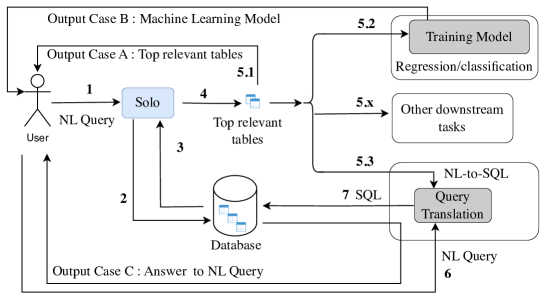
Figure 1. Solo and downstream tasks

2. Preliminaries

In this section, we present the the scope of data discovery (Section 2.1) , and then the problem statement (Section 2.2), followed by the related work (Section 2.3) and their shortcomings, and finishing with the challenges our work tackles in Section 2.4.

2.1. The Scope of Data Discovery

Our goal is to design a system that takes input natural language (NL) questions and returns tables satisfying users’ information needs. NL questions can be exceedingly complicated. Here, we target factual questions (Gardner et al., 2019; Iyyer et al., 2014), which are sufficiently expressive to let users discover interesting tables over large repositories. When questions may benefit from several tables, these tables will tend to be higher up in the ranking. Our system’s scope is identifying tables relevant to users’ information needs without assuming how those tables will be used. For that reason, we do not explore the application of techniques like question decomposition (Min et al., 2019; Perez et al., 2020; Zhang et al., 2019) which can be applied to complex questions at inference time to obtain simpler ones that can then be fed to our system. Solo, the system we introduce, is a discovery system that sits upstream to the applications users run to solve their tasks. We illustrate this in Fig. 1, where a NL-to-SQL system is used downstream of Solo: Solo finds a relevant table given a question, and then the NL-to-SQL system finds the answer to the question within that table.

2.2. Problem Statement

A table (relation), $T_{i}$, has a schema $\mathcal{R}$ with $k$ columns $C_{1},C_{2},...,C_{k}$ and rows, $r\in T_{i}$. The table may have a title (caption) and column names may be missing. A table collection is defined as a set of tables, $\mathrm{T}=\{T_{1},T_{2},...T_{N}\}$. A cell is indexed by a row $r$ and a column $c$, and the function $cell_{i}(r,c)$ returns the content of the cell in row $r$ and column $c$ of table $T_{i}$.

Given a question $q$, the problem we solve is to find a table $T_{i}^{*}$ among a large table collection $\mathrm{T}$, such that $T_{i}^{*}$ contains a cell $cell_{i}(r,c)$ that answers $q$. This means we do not target more complex question answering scenarios that require combining information from multiple tables.

Example 3/3. The City of Chicago Open Data Portal has about 630 tables. Today, users input keywords and obtain a ranking of relevant tables. Users can then inspect the table schema and values to determine if the table is indeed helpful to their needs. Our problem statement takes a natural language question as input instead of keywords, and returns a ranking of relevant tables, just as today’s search portals such as Socrata (Kalinin et al., 2022) and Open CKAN(openckan, 2023).

2.3. Related work

Table Question Answering. Question answering over tables (Table QA) models like TAPAS (Herzig et al., 2020), Tabert (Yin et al., 2020b) and Tapex (Liu et al., 2021) take 1 question and 1 table as input and return the cell that answers the question. Our system is complementary as it takes a collection of tables and returns the table necessary to answer the question. Both approaches can be combined if one wishes to directly obtain the answer for the question, although in practice analysts want to understand the table from where the answer is obtained to build trust on the result.

Table Search. The ad-hoc table search task in information retrieval (Zhang and Balog, 2018; Sun et al., 2019; Chen et al., 2020) also tries to solve data discovery problems but focus on key-word search which often have many relevant tables while our task needs to identify the table that can answer an input question and so needs more accurate relevance modeling.

Learned Data Discovery Systems. More recently, GTR (Wang et al., 2021) uses graph representation learning to model the relevance between a question and a table, retrieving the table with the highest relevant to a question. However, this model does not scale to a large collection of tables because computing the relevance is expensive and must be done for each table. Our contribution, Solo, first retrieves a small collection of relevant tables, and then applies a relevant model on this subset. A relevant approach is OpenDTR (Herzig et al., 2021) which learns a dense question and table encoder for large scale table search. However, OpenDTR requires expensive human-annotated data to perform well, so do the non-scalable relevance models.

Natural Language to SQL (NL-to-SQL). NL-to-SQL approaches aim to provide a NL interface to databases (Hristidis et al., 2003; Zhong et al., 2015; Popescu et al., 2004; Guo et al., 2019) for query answering. To this end, they translate a NL query to a SQL statement which is executed by a SQL engine to get the answer to the query. One of the challenging subtasks of a NL-to-SQL system is schema matching, necessary to map NL to valid table and column names (Katsogiannis-Meimarakis and Koutrika, 2023). In existing NL-to-SQL benchmarks, datasets often contain a small number of tables and also each query often includes the table names which makes finding the right tables trivial, e.g. there are only 5 tables on average per each database in the impactful Spider (Yu et al., 2018) dataset. In contrast, data discovery systems such as Solo aim to find a relevant table among tens of thousands of tables. In summary, NL-to-SQL approaches concentrate in solving query answering, while Solo concentrates in addressing data discovery.

Large Language Models (LLM). LLMs such as GPT-4 (OpenAI, 2023) answer input questions from a static collection of data, but, despite recent progress in that direction, it is harder to use them to answer questions over newly incorporated data because retraining them is prohibitively expensive. In addition, they are incapable of indicating what input tables (or data) were used to answer a prompt, which is necessary in discovery scenarios so users understand the provenance of the results. Solo adapts quickly to new repositories using the new self-supervised technique, and its answers exactly determine what tables contain the answer to the input question.

Retrieval-based question answering over documents (RQA). This class of systems concentrate on query answering over textual documents, as opposed to relational data. RQA approaches often include two components, a retrieval and a reader (Chen et al., 2017). The retrieval gets top k documents from large repositories so that the reader can output answers quickly (Karpukhin et al., 2020). Nowadays the reader is often implemented by a LLM and much work is about how to combine the retrieval and LLM for best performance (Izacard and Grave, 2020b; Lewis et al., 2020; Borgeaud et al., 2022; Mialon et al., 2023). For example, RAG (Lewis et al., 2020) uses a dense document retriever to augment a seq2seq language model and trains them jointly to output the best answer. But RQA concentrates on documents and not tables. Applying RQA to relational data discovery requires addressing the challenges of table representation (as documents) and table (document) ranking which are not trivial if human-annotated (question, table) pairs are unavailable. These are precisely the challenges our work addresses.

Scaling laws for neural models. The performance of neural models largely depends on three factors(Kaplan et al., 2020): model size, training data size and compute budget. A lot of work (Kaplan et al., 2020; Ghorbani et al., 2021; Alabdulmohsin et al., 2022; Bahri et al., 2021; Cherti et al., 2023) has shown that there is a power-law relationship between the performance and any of three factors. That means increasing model size, training data size or compute budget results in diminishing returns in performance. We observe similar trends during training, even though it remains difficult to write a concrete formula for determining when to stop training. Instead, to save compute budget, we combine Bayesian incremental training and self-supervised approach to automatically determine the appropriate training dataset size as described in Section 3.2.

2.4. Challenges of Learned Discovery Systems

Existing learned discovery systems suffer from several shortcomings that delineate the challenges we tackle in this paper.

C1. Collecting training data. Learned discovery systems trained on a table collection do not perform well in new table collections, so they have to be freshly trained for each table collection. Collecting training data is expensive and a major limitation of learned discovery systems. For example, OpenDTR uses 12K <question,table-with-answer> pairs. The challenge is to avoid the manually intensive task of collecting and labeling training data and deciding how large the training dataset should be to become representative and thus lead to a system that performs well on the target table collection.

C2. Table Representation. Learned discovery systems represent tables as vectors. OpenDTR uses TAPAS (Herzig et al., 2020) to represent a table with a single vector. As we show in the evaluation, the sparse and simpler BM25 model sometimes outperforms TAPAS. More recently, GTR (Wang et al., 2021) represents tables as graphs, similar to other efforts in data managements such as EmBDI (Cappuzzo et al., 2021) and Leva (Zhao and Fernandez, 2022). However, the graph construction depends on the order of rows and columns, which has no meaning in relations. Table representation has a big impact on system performance. Thus, the challenge is to find a dense table representation that outperforms sparse models and that works well on relations (C3).

C3. Relevance Model. The model computes a question representation and measures the relevance of different tables with respect to the question. The model must be designed in tandem with table representation (C2). The challenge is to find a relevance model appropriate for relations that performs well empirically when trained with synthetically generated questions (C1).

3. Self-supervised Training Data Collection

In this section, we present the new self-supervised strategy for training learned discovery systems, thus tackling challenge C1. Creating a training dataset requires solving two problems; we introduce novel strategies to address them:

• Generate question - table pairs. We introduce a strategy to automatically generate pairs of questions and the tables with the answers (Section 3.1).

• Determine training dataset size We introduce a strategy to determine when the size of the training dataset is sufficient to train the system (Section 3.2).

Throughout this section, we assume the existence of two additional components, a table representation component and a semantic relevant model component, that are needed to create the training dataset. Here, we treat these two components as black boxes. Then, in the next section, we provide the details of their design and implementation.

3.1. Synthetic Question Generation

A training dataset consists of positive and negative samples of question-table pairs. We first explain how to generate positive samples. We explain how to collect negative samples in Section 3.1.6.

The goal is to obtain a collection of question and table pairs, <$q,T_{i}^{*}$>, where $q$ can be answered with $T_{i}^{*}$. To automatically generate natural questions from tables a simple, yet problematic, approach is to define question templates and then fill in the templates with data from the tables. Unfortunately, this approach does not lead to diverse questions, which are needed to increase the matching of questions written by users, who may write questions very different than the templates.

Instead, we exploit the following observation. Large language models excel at giving diverse natural language interpretations of a SQL query, so we first generate SQL queries from tables and then translate those SQL queries to natural language. Specifically, our strategy consists of 3 different stages that we explain next: i) design a SQL template structure; ii) generate SQL queries from tables; iii) translate SQL queries to natural language.

3.1.1. SQL Template Structure.

We generate SQL queries that match the structure of factual questions; those answered with one table and that do not require complex processing and reasoning. More precisely, given a table $T_{i}$ that represents an entity $E_{i}$ with attributes $E_{i}.A_{1}$ , … , $E_{i}.A_{m_{i}}$, the answer to a factual question exists in some $E_{i}.A_{j}$ whether raw or via an aggregation operator such as $(Max,Min,Avg,Count)$. Factual questions are those that can be answered by search engines using a knowledge base (West et al., 2014). We use this format to drive the design of SQL templates, which are generated by applying the following rules:

• Randomly include an aggregation operator, MAX, MIN, COUNT, SUM, AVG on numerical columns.

• Include $\geq 1$ columns with predicates of the form “= < > ”.

• Do not include joins as we seek a single table that answers $q$.

In generating questions we strive for including sufficient context and for making the questions sufficiently diverse to resemble questions posed by real users. In more detail:

Context-rich queries. Whenever available, we include the table title with certain probability (as detailed below) as a special attribute (column) “About” to generate questions. This is because the table title often incorporates useful context. Consider the question “Where was he on February 19, 2009?”. This cannot be answered because we do not know what “where” refers to and who is “he”. The question, however, makes more sense if a table titled “List of International Presidential trips made by Barack Obama” can be integrated. We do not always include the title because it causes the learning procedure to overemphasize its importance and ignore the table schema. Instead, we introduce the title with certain probability $\alpha$. If a SQL query contains $m$ attributes in the predicates, we include the title with probability $\alpha=1/(m+1)$: more attributes means more context is already available so the title is less likely helpful.

Diverse queries. We want synthetic questions to resemble those posed by users. One way to achieve that is to ensure the questions represent well the attributes contained in the tables. To achieve that, we control how many predicates (referring to different attributes) to include in each question by sampling at most $m$ attributes. In addition, if the “About” attribute from above is included, it makes a question refer to as many as $(m+1)$ attributes.

3.1.2. Generation Algorithm

The generation algorithm must: i) deal with dirty tables; ii) sample to avoid generating humongous training datasets when the number of tables in the input is large. We first explain the strategy to deal with these two challenges and then present the algorithm.

Dealing with dirty data. Dirty tables in our context are those that become hard to generate SQLs from. They include those with missing column names and cell values with too long text. They are common in open data repositories (Cafarella et al., 2008; Herzig et al., 2021) and even enterprise scenarios. A cell with too long text is a problem when translating from SQLs to questions because the translation model we are using allows 200-300 words at most as input. Cells with text longer than $Q3+1.5(Q3-Q1)$, where $Q1$ and $Q3$ are the first and third quartiles of the distribution of text length, are discarded. When generating SQLs, the algorithm ignores columns without header names because the translation model asks for a relationship as input and the column name is the only option we have. Alternatively we can recover the headers using similarity search (Harmouch et al., 2021).

1 $SQLs=[]$

2 while len(SQLs) < batch_size do

3       $T_{i}=sample\_table(T)$

4       $sel\_col=sample\_columns(T_{i}.columns,1)$

5       $num\_cond=sample([0,..,Max\_Cond\_Num])$

6       $cond\_cols=sample\_columns(T_{i}.columns,num\_cond)$

7       $\alpha=1/(len(cond\_cols)+1)$

8       $use\_title=bernoulli.rvs(\alpha,1)$

9       if $use\_title$ then

10             $cond\_cols.append(TITLE)$

11      $agg\_op=sample\_aggre\_operator()$

12       $good\_rows=collect\_rows(T_{i},cond\_cols)$

13       if $good\_rows$ is not empty then

14             $r=sample\_row(good\_rows)$

15             $sql=create\_sql(r,sel\_col,cond\_cols,agg\_op)$

16             if sql not in $sql\_dict$ then

17                   $SQLs.append(sql)$ ; $sql\_dict.add(sql)$

18            

19      

return SQLs

Algorithm 1 $generate\_sqls(T,batch\_size,sql\_dict)$

Sampling strategy. We do not know how large the training dataset must be to achieve good performance. And extracting all possible SQL queries from a table collection would lead to too large datasets and infeasible training times. For example, consider a table collection with 100 tables, where each table has 10 columns and only 12 rows, we sample 4 columns per table and use only one aggregator operator. In this case, the number of unique SQLs is at least $100\cdot 12\cdot 10\cdot\left(\sum_{k=0}^{3}{{10}\choose{k}}\right)=2,112,000$. This number grows fast with more tables and rows. Training on so many questions requires more hardware resources and time and quickly becomes prohibitively expensive.

Instead, the generation algorithm uses a sampling procedure that is driven by the training process which asks for a collection of $batch\_size$ SQLs to be generated. This procedure is used by the incremental training strategy we introduce (Section 3.2) to determine when a training dataset is sufficiently large to achieve good performance on the task and thus stop. Now, within each invocation of the algorithm, we want to ensure that the $batch\_size$ SQLs generated cover the table collection well. We achieve that by using the following algorithm.

The Generation Algorithm. The algorithm combines 3 independent sampling procedures (Algorithm 1). The first samples tables. The second samples columns given a table, and includes one of the logical operators in the predicates. Then the $alpha$ probability is computed (line 1) to decide whether to include the table’s title. The third sampling procedure samples rows, given columns of a table. When columns are numerical, the generation algorithm samples one of the aggregate operators. In addition, and ahead of the sampling process, the algorithm makes an initial pass over the data to: i) determine column types; and ii) compute the distribution of cell text length, which is used to filter out outliers. The result of the algorithm is some number ($batch\_size$) of SQL queries used for training or validation.

3.1.3. Translation from SQL to question.

We use LLMs to translate SQL queries into natural language questions. Specifically, we use the T5 (Raffel et al., 2019) sequence-to-sequence model. T5 is pretrained on the “Colossal Clean Crawled Corpus” (C4) (Dodge et al., 2021), which includes internet documents from 365 million domains with 156 billion tokens. Although C4 is very large, it is mostly in natural language, and the pretrained T5 model learns a natural language to natural language mapping which is not directly applicable for our purpose. So we fine-tune T5 using WikiSQL (Zhong et al., 2017), a dataset with pairs of SQL queries and their corresponding natural language representation that has been previously used for tasks such as natural language question interface to relational databases  (Zhong et al., 2017).

SQL keyword	Custom T5 token	SQL keyword	Custom T5 token
select	[S-E-L-E-C-T]	where	[W-H-E-R-E]
avg	[A-V-G]	=	[E-Q]
max	[M-A-X]	>	[G-T]
min	[M-I-N]	<	[L-T]
count	[C-O-U-N-T]	and	[A-N-D]
sum	[S-U-M]

Table 1. SQL keywords for T5 model input

During fine-tuning, we update the weights of T5 without adding new layers. When encoding SQL statements, and to escape SQL keywords, we include these in brackets following a format that indicates the model they must be escaped, e.g., “where” becomes “[W-H-E-R-E]”. A complete list of keywords is shown in table 1; those keywords will never appear in the output questions.

3.1.4. Assigning $T_{i}^{*}$.

Large table collections contain table duplicates and near-duplicates. Consequently, a single question may be answered by more than a table. The approach considers any table that can answer a question as a valid solution, and thus it creates multiple question table pairs. To detect duplicates, our approach simply filters out tables with the same schema; it can be extended to use duplicate detection techniques (Fernandez et al., 2018; Koch et al., 2023) .

3.1.5. Validation data.

It is a best practice to sample validation data from the same distribution as the test data. However, this requires users to manually collect question and answer table pairs. Our goal is to not require manual labeling by users, which we achieve via the new self-supervised method. Now, we collect validation data in the same way we collect training data, using a holdout set that the system automatically creates on the input table collection.

3.1.6. Completing training dataset

The discussion so far has concentrated on generating positive samples of question-table pairs. Now we explain how to generate negative samples. The data is collected to train the relevance model that we explain in detail in Section 4.2. During test, the relevance model always takes as input a small set of tables from first-stage retrieval. To emulate the test scenario, given a synthetic question, the system calls the first-stage retrieval component to get a small set of tables and labels those tables not the source of the question as negative examples which are often called hard negatives (Schroff et al., 2015). If all tables are positive or negative we ignore this question. The first-stage retrieval does not retrieve all the cells for a table but some cells of it because of the table representation which we explain more in Section 4.1.

3.2. Bayesian Incremental Training

We introduce a strategy that increases the training dataset size incrementally until achieving good performance, thus, removing the need to select a training dataset size a priori.

Our idea is to apply a new Bayesian incremental training process (Kochurov et al., 2018). We first provide technical background on Bayesian Neural Networks and then present our incremental strategy.

3.2.1. Background on Bayesian neural networks.

Bayesian neural networks attach a probability distribution to the model’s parameters, thus paving the way to avoid overfitting and providing a measure of uncertainty with the answer. We leverage Bayesian neural networks for a different purpose, to learn when a model’s performance has reached a good quality and thus avoid keep feeding expensive to generate training data.

A general approach to learn the parameters $\theta$ of a neural network from dataset $D$ is to maximize the likelihood, $\tilde{\theta}=\operatorname*{argmax}{P(D|\theta)}$. This point estimation of the parameters often leads to overfitting and overconfidence in predictions (Jospin et al., 2022). To address this issue, Bayesian neural networks (Jospin et al., 2022; Blundell et al., 2015) learn a posterior distribution over $\theta$ using the Bayes rule.

$$P(\theta|D)=\frac{P(D|\theta)P(\theta)}{P(D)}=\frac{P(D|\theta)P(\theta)}{\int_{\theta}P(D|\theta)P(\theta)d\theta}$$

At inference time, the prediction is given by taking expectation over $P(\theta|D)$,

$$P(y|x)=\mathbb{E}_{P(\theta|D)}(P(y|x,\theta))$$

In practice, a list of $\theta_{1},\cdots,\theta_{m}$ are sampled from $P(\theta|D)$ and the prediction is made using bayesian model averaging (Wilson and Izmailov, 2020),

$$P(y|x)=\frac{1}{m}\sum_{i=1}^{m}P(y|x,\theta_{i})$$

While it is easy to define a network for $P(D|\theta)$, such as the multilayer perceptron (MLP), and specify a prior for $\theta$, such as an isotropic gaussian, the posterior distribution $P(\theta|D)$ is computationally intractable because of the integration over $\theta$. To address the intractability, variational learning (Blei et al., 2017) uses another distribution $q(\theta|\varphi)$, parameterized by $\varphi$ to approximate $P(\theta|D)$. Variational learning optimizes $\varphi$ to minimize the KL divergence of $P(\theta|D)$ and $q(\theta|\varphi)$. We use Bayesian neural network to train the relevance model given a list of datasets $D_{1},...D_{m}$.

3.2.2. Bayesian Incremental Training Strategy.

The goal is to learn recursively a posterior distribution $P(\theta|D_{1},...,D_{t})$ over the neural network parameters $\theta$ given a prior distribution $P(\theta|D_{1},...,D_{t-1})$ and only one dataset $D_{t}$. The prior distribution $P(\theta|D_{1},...,D_{t-1})$ contains the knowledge the relevance model learns from previous datasets so that the model does not have to start training from scratch and uses $D_{t}$ only. This is the key to the efficiency gain.

Because the posterior distribution $P(\theta|D_{1},...,D_{t})$ is intractable to compute, we use $q(\theta|\varphi)$, parameterized by $\varphi$ to approximate the posterior and then optimize $\varphi$ using backpropagation (Blundell et al., 2015),

$$\tilde{\varphi}=\operatorname*{argmin}{\sum_{i=1}^{m}\log{q\left(\theta^{i}|\varphi\right)}-\log{P\left(\theta^{i}\right)}-\log{P\left(D|\theta^{i}\right)}}$$

Where $\theta^{i}$ is a sample from $q(\theta|\varphi)$ and $P\left(D|\theta^{i}\right)$ is determined by the relevance model (see Section 4.2). Next, we discuss the choice of $q(\theta|\varphi)$ and $P(\theta)$ and also some techniques to speed up training.

The approximate distribution, $q(\theta|\varphi)$ . In the relevance model (see next section) $\theta$ = {($\boldsymbol{W_{i}}$ , $\boldsymbol{b_{i}}$)}, where $\boldsymbol{W_{i}}$ and $\boldsymbol{b_{i}}$ are the weight matrix and the bias vector for layer $i$. To simplify and speedup computation, we follow the approach in (Blundell et al., 2015) and assume that each weight and bias is an independent gaussian variable with mean $\mu$ and standard deviation ${\sigma}$, so that $q(\theta|\varphi)$ can be fully factorized. More concretely, random noise $\epsilon$ is sampled from the unit gaussian $\mathcal{N}(0,1)$, and ${\sigma}$ is derived by $\sigma=\log(1+\exp(\rho))$ and then a sample weight $w$ in $\boldsymbol{W_{i}}$ is given by $w=\mu+\sigma\cdot\epsilon=\mu+\log(1+\exp(\rho))\cdot\epsilon$. So the parameter $\varphi$ is the set of $(\mu_{j},\rho_{j})$.

To initialize $\mu_{j}$, we sample uniformly from $(-1,1)$. To initialize $\rho_{j}$, we sample uniformly from $(-3,0)$ and this makes the initial $\theta_{j}$ sit in the range $(0.05,0.7)$. Smaller initial $\theta_{j}$ for each weight/bias would make training much harder to converge.

The prior $P(\theta)$ . We only have to specify a prior for the first dataset $D_{1}$. After training is done with $D_{1}$, the posterior $P(\theta|D_{1})$ is the prior for the next training and so on. Then both the prior and posterior are gaussian distributions. In particular, the initial prior is a gaussian with mean $0$ and standard deviation $1$ for each weight or bias, which is consistent with the initialization of the parameter $(\mu_{j},\rho_{j})$. In addition, in our scenario, an inaccurate initial prior is not an issue because there are many training data points and as the training data increases, the impact of the initial prior plays a lesser role.

Speedup of training and evaluation. First, we train the Bayesian neural network by sampling $\epsilon$ once per batch (as opposed to $n$ times as in other context), thus speeding up the training process without losing accuracy. Sampling $n$ times is usually done to conduct model averaging: we achieve the same effect by sampling across iterations. Second, on validation data, we use the posterior gaussian mean of weights/bias for prediction instead of doing bayesian model averaging, further reducing time. Together, these optimizations improve the training time of the Bayesian neural network, making it substantially faster than the baseline approach.

4. Table Representation and Relevance Model

In this section, we present the strategy for representing tables as vectors (Section 4.1) and the semantic relevance model (Section 4.2), tackling challenges C2 and C3.

4.1. Table Representation

The goal is to find a table representation that facilitates matching with questions, thus addressing Challenge 2 (C2).

We represent each table as a graph, where the nodes are the subject and object of every (subject, predicate, object) triple in the table. The intuition is that a natural question that can be answered with a table can be answered with a collection of triples from that table. Hence, representing the table via its triples facilitates matching it with relevant questions during first-stage retrieval. There are two advantages to representing tables as triples. First, a triple represents a basic relationship. By representing tables with its triples, we obtain a more fine-grained representation than state of the art models such as OpenDTR, which treats a table as a whole. Second, it is easier to treat a triple as text than it is to treat a table, so we can use any off-the-shelf text encoders to transform triples into their vector representation. Next, we provide an example first, present the new row-wise complete graph method for table representation, and finish with encoding.

Example. Consider the running example "What are the business hours of Employment Resource Center at Howard?", and the table that answers this question, $T_{i}^{*}$, shown in Fig.  2. The question contains two triples: (Employment Resource Center, at, Howard) and (Employment Resource Center, business hours, ?) , where the placeholder “?” corresponds to the answer. At the same time, the table contains two triples related to the question:

• (Employment Resource Center , Facility - Street Address , 1623 W. Howard) denoting the relationship between Facility and the Street Address column, i.e. Employment Resource Center is located at Howard street, which is close to (Employment Resource Center, at, Howard) in the question.

• (Employment Resource Center , Facility - Hours , M-F: 9AM-5PM; SA: 9AM-1PM) denoting the relationship between Facility and Hours columns, with two column names connected by a hyphen is the predicate. This relationship is close to (Employment Resource Center , business hours , ?) implied in the question.

Matching triples is the mechanism our approach uses to identify direct matches between a question and a table.

Row-Wise Complete Graph (RCG). Representing a table as triples is common practice in the semantic web (Allemang et al., 2020) community. One challenge of doing so is to identify correctly the entity and relationships the table represents. With an entity-relationship diagram available (assumed known for semantic web), this is straightforward, but we do not have access to those in discovery scenarios with large collections of tables. Instead, we use a complete graph to connect each pair of cells in each row in the table, as shown in the Fig. 2. Furthermore, the table title is included as a special column of each table, thus it is also represented in triples for every row. In such complete graph, some edges will be spurious, while others will match the table question, as shown in the example. We are not concerned with the spurious relationships because the first-stage retrieval will filter some out if they do not match any question, and the relevance model in Section 4.2 will learn to distinguish more. We show empirically in the evaluation the benefits of such a representation. Next we explain how to encode the graph for first-stage retrieval.

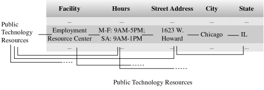
Figure 2. Example of Row Wise Complete Graph (RCG)

Encoding. In this last step, the goal is to encode each triple (edge) from the graph produced by RCG. First we convert each triple into a snippet of text. Specifically, a triple text always begins with the table title and is then followed by column name and cell value of subject and object. Double quotes and commas are added to indicate the boundary. E.g. The triple text for (Employment Resource Center , Facility - Hours , M-F: 9AM-5PM; SA: 9AM-1PM) is "Public Technology Resources" , Facility "Employment Resource Center" , Hours "M-F: 9AM-5PM; SA: 9AM-1PM". Second, to encode the tripe text, we use dense representations because we found they outperform sparse representations based on TF-IDF and BM25, as we show in the evaluation section. We use vector representations provided by a student dense retrieval model distilled from a pre-trained teacher dense retrieval over text ((Izacard and Grave, 2020a)), we leave why and how to distill the student model to Section 5 . The student model contains a question encoder (which we use to encode questions) and a passage encoder to encode the triples. The resulting dense vectors for triples are then indexed for first-stage retrieval.

4.2. Relevance Model

We design a relevance model to solve the second-stage ranking problem, thus addressing Challenge 3 (C3). Given a question, $q$, the first-stage retrieval returns $K_{u}$ triples arising from $K_{t}$ tables (there may be multiple triples from the same table). The goal of second-stage ranking is to choose one table $T_{i}$ from $K_{t}$. The general idea is to match $q$ to triples from $T_{i}$. To do so, we use a pretrained QA model over text (Izacard and Grave, 2020a) to match $q$ to each triple, and then construct a matching representation ($q$ ,$T_{i}$). The QA model takes a question and a text representation of a triple and outputs a matching representation. We employ two techniques to boost the matching: triple annotation and representation augmentation.

Triple annotation. We use the pretrained QA model over text (Izacard and Grave, 2020a) to provide input features for each (question, triple) pair. To use the QA model, we convert triples to text, but this transformation to text is different than the performed during first-stage retrieval. Here, we seek to annotate the triple to improve its context which, in turn, helps with ranking as such context often includes sufficient information for the model to resolve semantic differences between words. To improve the context, we use special tags to indicate the role of each string element in the triple and in the table. For example, consider the aggregation question: "Which public technology resource in Chicago has the longest hours of operation?”. A triple in Fig. 2 that refers to the column “Hours” is more likely to answer the question than a triple from another table where the text “Hours” appears in a cell. We incorporate the context as part of the input fed to the QA model: [_T_] to denote the table Title; [_SC_] to denote subject column name $c_{x}$. [_S_] for $Cell(r,c_{x})$, which means Subject. [_OC_] for column name $c_{y}$, which indicates Object Column. [_O_] for $Cell(r,c_{y})$, which indicates Object.

When a triple involves two columns, we still include the table title as context. For example, the triple (Employment Resource Center , Facility - Hours , M-F: 9AM-5PM; SA: 9AM-1PM)) is annotated as “[_T_] Public Technology Resources [_SC_] Facility [_S_] Employment Resource Center [_OC_] Hours [_O_] M-F: 9AM-5PM; SA: 9AM-1PM”. In contrast, the triple (Public Technology Resources, Facility, Employment Resource Center) that only refers to one column is annotated as: “[_T_] Public Technology Resources [_SC_] [_S_] [_OC_] Facility [_O_] Employment Resource Center”. That is, “Public Technology Resources” works as title and subject.

Representation augmentation. We augment the representation by adding redundancy (Tobin et al., 2017), which is shown to reduce distributional shift and improve the matching process. A table is represented by the triples retrieved during the first-stage retrieval stage: $(q,\{p_{1},\cdots,p_{m}\})$. To augment that representation, we represent the pair $m$ times, including each time the question and each of the triples, i.e., $(q,\{p_{1},\cdots,p_{m}\})+(q,p_{i})\forall i\in m$. This redundancy helps to introduce diversity because they share the label.

Model. Given a question $q$ and $K$ annotated triples $p_{1},p_{2},\ldots,p_{K}$, we first feed all of them to the pretrained QA model to get a feature vector $X_{i}$ for each ($q$, $p_{i}$) pair, $X_{i}=qa\_enc(q,p_{i})$. We do not change the parameters of QA, so $X_{i}$ is fixed. We then project $X_{i}$ to a vector space w.r.t. table to get a vector $REP_{t}(q,p_{i})=W_{t}X_{i}+b_{t}$ and then apply element-wise max-pooling to all $REP_{t}(q,p_{i})$ vectors in the same table to get an $(q,T_{j})$ representation vector $REP(q,T_{j})$:

$$REP(q,T_{j})=Max\-Pool([REP_{t}(q,p^{T_{j}}_{1});REP_{t}(q,p^{T_{j}}_{2})...])$$

where $T_{j}$ indicates the table $X_{i}$ belongs to. Max-pooling helps select the best suitable triple $p_{i}$ for the question. To construct multiple relevance representation, each $X_{i}$ is projected to another vector space w.r.t. triple to get a vector $REP_{u}(q,p_{i})=W_{u}X_{i}+b_{u}$ which is concatenated with $REP(q,T_{j})$ to get multiple equivalent relevance representation $REP(q,p_{i},T_{j})$:

$$REP(q,p_{i},T_{j})=[REP(q,T_{j});REP_{u}(q,p_{i})]$$

Then a multilayer perceptron (MLP) (Goodfellow et al., 2016) layer is added to compute the relevance score $s(q,p_{i},)=MLP(REP(q,p_{i},T_{j}))$ and then a Sigmoid layer and Binary Cross Entropy is added to it to compute the maximum likelihood estimation $\log{P\left(D|\theta\right)}$:

$$\log{P\left(D|\theta\right)}=\sum_{i=1}^{m}(y_{i}\log\sigma(s(q,p_{i}))+(1\text{-}y_{i})\log(1\text{-}\sigma(s(q,p_{i}))))$$

where $y_{i}$ is the the 0/1 label. During prediction, tables are ranked according to a relevance score computed as $\max_{p_{i}\in T_{j}}REP(q,p_{i},T_{j})$. The larger the score the more relevant the table is to the query and thus the higher in the ranking the table will appear.

To make max-pooling more effective, the learned table-perspective representation $REP_{t}(q,p_{i})$ must be as different from each other as possible in a table because each $p_{i}$ is supposed to be a different triple in that table. To this end, we add a regularizer, the Diversity Regularizer to the final loss to minimizes the mean of mutual dot product of $REP_{t}(q,p_{i})$ in a table.

Summary of relevance type. Our relevance model ranks question/table relevance by using the feature vector encoded by the pretrained QA model (Izacard and Grave, 2020a) and these vectors are good representation of word semantics. In addition we incorporate table context (see the “Triple Annotation” paragraph), that results in the relevance model ranking higher those tables that are semantically more related (according to the context) to the question. The output ranking reflects the relevance of tables with the question. When questions are ambiguous and the context is not sufficient to disambiguate the meaning of the question, those relevant tables make it into the ranking, letting users resolve the remaining ambiguity. To be robust to both context-rich and context-poor scenarios, our question generation strategy (see Section 3.1) samples different number of columns from a table and includes the title probabilistically, thus producing training datasets with different contexts. More columns with the title means more specific questions (more context), while fewer columns and no title means more ambiguous questions.

5. Solo Overview and Implementation

In this section, we first give an overview of our end-to-end system Solo to show how the components work together to solve the table discovery problem. The system is built in Python using around 5,000 lines of new code. The system contains a CLI and a UI interface for users to type questions and then show top $N$ tables in order of relevance to the question. Each result in the ranking is accompanied by the provenance of that table including what triples match the question, so users have an easier time understanding the results.

While building Solo to implement the self-supervised approach explained in the previous sections, we run into severe challenges that would render a learned discovery system impractical. Here, we explain those challenges and the optimizations we implemented to address them (Section 5.2). We start with an overview of Solo.

5.1. Overview

Fig. 3 shows the overview of Solo, which has an offline mode and online mode. In offline mode, tables are decomposed into triples (step 1) which are then encoded (step 2), and indexed (step 3). Then SQL queries are sampled from the target table collection (step 4) and then a SQL2Question module translates SQL queries (step 5) into synthetic questions which are encoded (step 6) and sent to a vector index (step 7, we use Faiss (Johnson et al., 2019) as it is scalable and supports similarity search). A small set of top triples are returned (step 8) for each synthetic question to train the relevance model (step 9). If the more training data is needed, the training data assembler sends a message (step 10) for more questions. In online mode, a real question is encoded (step t1) and sent to the vector index (t2). A small set of triples are returned and together with the question are sent to the released relevance model (t3) to predict the most relevant tables.

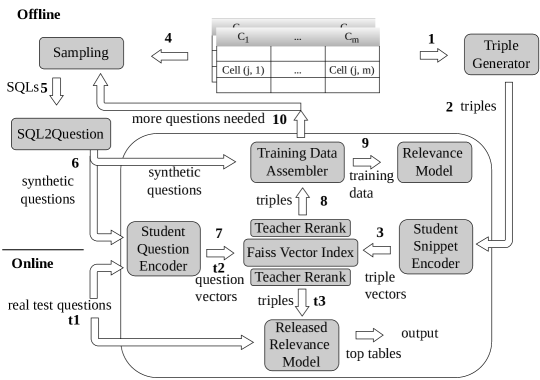
Figure 3. Overview of Solo

5.2. Key challenges and solutions

A dense first-stage text retrieval encodes questions and text snippets (triple text in our case) separately so that the large amount of text snippets in a corpus can be pre-encoded before query. However, existing off-the-shelf pre-trained dense retrievals are often very expensive because of the transformer architecture (Vaswani et al., 2017) with many layers and so encoding can take very long time given a large amount of triples. As an example, in the City of Chicago Open Data Portal, although the number of tables is not large, some tables have as many as 10 millions of rows and in total will result in around 42 billion triples. We experiment with 20 million triples on a single NVIDIA Quadro RTX 6000 GPU node and use the state-of-the-art FiD dense retrieval (Izacard and Grave, 2020a) the version pre-trained on TriviaQA (Joshi et al., 2017), a high-quality dataset with 95K question answer pairs with evidence documents. It takes around 6 hours to finish the encoding. To encode all 42 billion snippets of this dataset would take a prohibitive amount of 525 days. Using cloud GPUs to parallelize encoding is an expensive option. For example, at the time of this paper, Lambda (lambdalabs, 2023) offers the Quadro RTX 6000 instance with $0.5/h, and to finish the encoding of 42 billion snippets in one day with 525 GPUs (often you are not allowed to launch so many instances) would cost 525 x 24 x 0.5 = $6,300. Then either the user spends more money on machines or waits more time for encoding. So the first challenge is to implement a light encoder without affecting the system accuracy.

Another major challenge with dense vector representation is the storage footprint of the resulting vectors. Often each triple is encoded into a high dimensional vector of 768 floating point numbers. If each number is stored with 16-bit float precision, a vector will use $768\times(16/8)/1024=1.5$ k storage and 42 billion vectors will take up around 60T. This is clearly beyond the capacity of many organizations that would otherwise benefit from learned discovery systems. The second challenge is to reduce storage size without affecting the system accuracy. Now we describe the solutions.

5.2.1. Light dense retrieval.

It contains two components:

Student encoder. To get a cheap encoder, we use knowledge distillation (Hinton et al., 2015) which uses the heavy Fid encoder (the teacher) to guide the training of a light student encoder. So the student encoder is supervised both from the TriviaQA data label (used for training the teacher) and the scores from the teacher on TriviaQA. In Fid, there is only one encoder for both question and passage. To minimize the accuracy drop during distillation, we use two with the student question encoder the same model architecture as Fid but the student text snippet encoder having only 1 layer versus 12 layers in Fid. With this design, we get around 5x speedup in encoding. Another bottleneck of encoding is tokenization (on CPU) of input text which uses time close to the student model inference (on GPU) time. We then use multi-threading and the result student encoder is around 10x faster than the teacher also with multi-threading.

Teacher to rerank. To compensate for the accuracy drop by the cheap student encoder, we use the teacher to rerank the n snippets from the student and output the top k ones to the relevance model.

5.2.2. Reduce storage size

To reduce the storage, we use product quantization (Jegou et al., 2010) where each vector is split into m (divisible by 768) parts and each part is an identifier (1 byte) of one of 256 clusters. The compression ratio is then (768*2+8)/(m+8) $\approx$ 768*2/m where the 8 bytes is the integer triple ID. To achieve comparable retrieval accuracy. E.g. with m=384, the student needs to retrieve n=1,500 triples for the teacher to rerank and 3,000 for m=256. More triples with smaller m will make the teacher rerank more expensive and also accuracy drops quickly. So m=384 is used by default, thus using 1/4 of the storage footprint.

6. Evaluation

In this section, we answer the main research questions of our work:

$\bullet$ RQ1. Does self-supervised data discovery work? The main claim of our work is that learned discovery systems need repository-specific training data to perform well, and that our self-supervised approach can collect that data automatically. We measure the extent to which systems suffer when not specifically trained for a target repository and we measure the performance of our approach. We will compare with strong baselines to contextualize the results. This is presented in Section 6.1.

$\bullet$ RQ2. Does Bayesian incremental training work? A challenge of producing the training dataset is to choose its size. Too large will lead to unnecessary resource consumption without any accuracy benefits and possibly a degradation. Too small will lead to underperforming models. The technique we introduce uses Bayesian neural networks to know when to stop. We evaluate its effectiveness here when compared to a baseline approach that retrains iteratively using ever larger datasets. This is presented in Section 6.2.

$\bullet$ RQ3. How does table representation affect accuracy? An important contributor to the end to end performance is the representation of tables. We argued in the introduction that many existing approaches do not work well and thus we introduced a new row-wise graph based approach. See Section 6.3.

$\bullet$ RQ4. Microbenchmarks To provide a full account of the performance of the end to end system we include microbenchmarks that concentrate in answering two questions: the performance differences of using sparse vs dense indices during the first-stage retrieval, and the runtime performance of the new approach, accounting for both offline and online components. See Section 6.4.

Metrics. The ultimate goal is to identify the table that contains the answer to an input question. To measure the accuracy of the different baselines when given a set of questions we use the precision-at-K metric (P@K) aggregated over all questions, as in previous work (Herzig et al., 2021). This metric indicates the ratio of questions for which the answer is in the top K tables. We measure P@1 and P@5. We do not use recall@K because in the benchmarks we use, each question has 1 single table as the answer. More specifically, in one benchmark there is exactly one table per question, while in the other only 7 questions out of 959 have 2 valid answer tables. Thus, measuring precision alone is sufficient to understand the quality of the approaches we compare.

Datasets. We use two benchmark datasets that have been extensively used by previous systems and that have been generated from real-world representative queries.

$\bullet$ NQ-Tables (Herzig et al., 2021) This dataset contains 210,454 tables extracted from Wikipedia pages and 959 test questions which are a subset of the Google Natural Questions (Kwiatkowski et al., 2019). It is very popular in table retrieval (Shraga et al., 2020; Pan et al., 2021; Herzig et al., 2021) because the questions are asked by real Google Search users. The tables are relatively dirty, with 23.3% tables having some column header missing and 63% tables having cells that contain long chunks of text.

$\bullet$ FetaQA (Nan et al., 2022) This dataset contains 10,330 clean tables from Wikipedia and 2003 test questions. The questions are generally longer and more complex than those from NQ-Tables.

System Setup. We run all experiments on the Chameleon Cloud (Keahey et al., 2020). We use one node with 48 processing threads, 187G RAM, and an NVIDIA RTX 6000 GPU. The OS is Ubuntu 18.04 and the CUDA version is 11.2 and 10.2 (for other baselines). The system is implemented in Python v3.7.9 and uses pytorch 1.12.1.

6.1. RQ1. Self-supervised data discovery

We measure the P@1 and P@5 accuracy of the self-supervised discovery system ( that uses the synthetically generated training data ) on the two benchmark datasets. To interpret the results, we compare them against the following baselines:

BM25 (Table-Row-Tokens). Discovery systems such as Aurum (Fernandez et al., 2018) and Auctus (Castelo et al., 2021) use traditional information retrieval techniques based on BM25 to retrieve tables given keywords. We implement this baseline to represent these discovery solutions. In particular, we index every row of a table, along with the table’s title in Elastic (elasticsearch, 2023).

Tabert. (Yin et al., 2020b) is pretrained on 26 million tables with corresponding free text context. It does not solve data discovery, instead it answers questions by pointing to the cell of a given input table. Still, we use this model to understand if its table representation works for data discovery. We emphasize that Tabert encodes a question and table pair simultaneously and thus does not scale to large repositories of tables. We use our first-stage retrieval system to get a small set of tables as candidates. And then we use Tabert to output a question embedding and a column embedding for each column in a table. We use the mean column embedding and compute the cosine similarity score of the question and mean column embedding to rank tables.

OpenDTR. (Herzig et al., 2021) is a state-of-the-art learned discovery system. We use 3 variants: OpenDTR-Retrain, OpenDTR-NoRetrain and OpenDTR-Synthetic.

$\bullet$ OpenDTR-Retrain is retrained on a human-annotated training dataset that has the same distribution as the test dataset. For example, when the target test dataset is NQ-Tables, OpenDTR-Retrain is trained on NQ-Tables. This baseline requires collecting training data for each dataset and is thus not desirable. Still, we include it because it allows us to understand the performance difference between (expensive) human-collected training datasets and our approach.

$\bullet$ OpenDTR-NoRetrain is the system instance pretrained on a human-annotated training dataset having different distribution from the test dataset. For example, when the test dataset is NQ-Tables, OpenDTR-NoRetrain means the system instance trained on FetaQA. This baseline helps us understand what happens to the system performance when a learned discovery system is deployed on a new table collection without retraining.

$\bullet$ Finally, OpenDTR-Synthetic is trained on the synthetic questions generated by our self-supervised approach. We use this baseline to understand the impact of the new table representation and the semantic relevance model.

GTR. (Wang et al., 2021) is a state-of-the-art second-stage ranking model. Because it only solves second-stage ranking, we use our first-stage retrieval system to obtain results end-to-end. We implement 3 variants as before: GTR-Retrain, GTR-NoRetrain and GTR-Synthetic.

Experimental Setup. We train OpenDTR models using the released official code. In our system, we encode each triple as a 768-dimensional vector using the Fid Retriever (Izacard and Grave, 2020a) pretrained on the TriviaQA dataset. This results in 41,883,973 vectors on NQ-Tables, and 3,877,603 vectors on FetaQA. We index those vectors using Faiss (Johnson et al., 2019). We retrieve at least 5 tables during first-stage retrieval and then apply the second-stage ranking. We use the original code to train the GTR models. We train our system, OpenDTR-Synthetic and GTR-Synthetic using the exact same set of training data produced in a self-supervised manner.

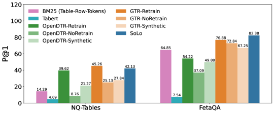
Figure 4. P@1 Accuracy on baseline datasets

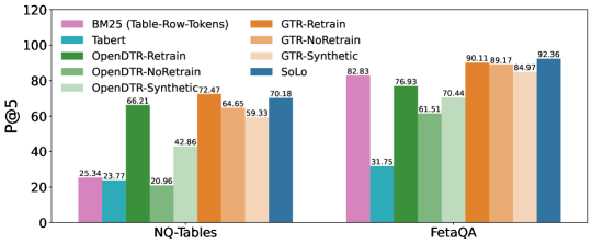
Figure 5. P@5 Accuracy on baseline datasets

6.1.1. Main Results

We show the P@1 and P@5 in Fig. 4 and Fig. 5, respectively. We highlight several key insights:

Baselines underperform on new table collections when not specifically retrained. The first observation we make concerns OpenDTR-NoRetrain and GTR-NoRetrain. When these systems are trained with data from one benchmark and evaluated on the other, their performance deteriorates significantly, by 30 and 18 points in the case of OpenDTR on NQ-Tables and FetaQA, respectively. And by 20 and 4 points in the case of GTR-NoRetrain. This demonstrates that without retraining, a learned table discovery system vastly underperforms on new table collections.

Off-the-shelf pretrained Table QA representation does not generalize to table discovery. The very low accuracies of Tabert show pretrained embeddings in table scenario are hard to applied to related tasks and training is needed to get good performance.

Solo produces synthetic training datasets that achieve high accuracy. Solo vastly outperforms non-trained systems. Compared to the NoRetrain variants, Solo achieves 30 and 15 more points than OpenDTR-NoRetrain and GTR-NoRetrain in NQ-Tables and 40 and 13 more points in FetaQA. This improvement in accuracy comes at the same cost for the human, who does not need to collect data and label it manually because our approach does it for them. This result validates the main contribution of our paper.

Solo is competitive in performance compared to the retrain baselines without needing to pay the cost of obtaining a new training dataset. Even when compared to the other baselines retrained on benchmark-specific training datasets, Solo achieves good performance. In fact Solo outperforms OpenDTR-Retrain in both datasets by 3 and 25 points in NQ-Tables and FetaQA respectively. It also outperforms GTR-Retrain in the FetaQA benchmark by 6 points. It underperforms GTR-Retrain in the NQ-Tables dataset by only 3 points, but again, to emphasize, without paying the cost of collecting data manually.

Solo always outperforms BM25, but this is not true for the other baselines. BM25 represents the retrieval performance of non-learned discovery systems. Note that OpenDTR-NoRetrain underperforms BM25 in NQ-Tables by 6 points. This means that, without our approach, and without the ability to collect a new dataset, a non-learned data discovery solution will outperform the more sophisticated OpenDTR. Or rather, that collecting high-quality training data is decidedly important for learned table discovery to perform well on new table collections. GTR does better than OpenDTR when compared to BM25—recall it uses our new first-stage retrieval. In contrast, Solo always outperforms BM25.

Solo performance benefits go beyond the synthetic data generation. To test this hypothesis and evaluate the contributions of the new table representation and relevance model we use the same synthetically generated dataset produced by our approach to train all baselines and compare their performance; this corresponds to the Synthetic baselines. As shown in the figures, when all baselines are trained on the synthetically generated dataset, Solo outperforms every other baseline by 20, 15, 33, and 15 points (from the left to the right of the figure). These results validate the design of the table representation and retrieval model.

The trends are similar and accentuated when measuring P@5. The trend when observing P@5 is the same as in P@1, with the total accuracy much higher, as expected. This suggests that when the end user has the bandwidth to manually check a ranking of 5 tables that may answer their question, they are much more likely to identify the answer they are after.

6.1.2. In-depth analysis of results

We ask: Why do the Retrain baselines perform worse than Solo despite having access to high-quality manually collected training data?. When analyzing the logs for the FetaQA benchmark, we find that Solo performs better at matching entities in the question and table at the word level. This is largely because Solo takes advantage of the OpenQA (Izacard and Grave, 2020a) model which is pretrained on the TriviaQA (Joshi et al., 2017) question dataset. The same reason applies to OpenDTR-Retrain. Note, it is common practice nowadays to transfer knowledge from a model pretrained on high-quality human data (Qiu et al., 2020); but this is orthogonal to Solo’s users, who do not need to annotated data manually.

On NQ-Tables (where Solo underperforms GTR-Retrain), we find Solo is more likely misled by long cells that contain information related to the question, while GTR-Retrain performs better in exploiting the table cell topology structure to find the ground truth table. We use an indicative example from our logs. Given the question “where is hindu kush mountains located on a map”, Solo chooses a table with a long cell text “The general location of the Himalayas mountain range (this map has the Hindu Kush in the Himalaya, not normally regarded as part of the core Himalayas)”. The text does indeed contain an answer. In contrast, GTR chooses a table with a cell containing “Hindu Kush” and a cell containing the coordinates, which gives a more precise answer and is what the benchmark was expecting. It is arguable whether one answer is indeed superior to the other for an end-user, but it is certainly the case the benchmark favors GTR in this case. Finally, because FetaQA is a relatively clean benchmark and most cells contain simple information, we do not see the same effect in this dataset, i.e., Solo is less likely to select a long cell and it consequently outperforms GTR-Retrain and OpenDTR-Retrain. Note that in any case, the performance of Solo, which is close to the other baselines, is achieved without any human-collected dataset.

Why do the Synthetic baselines underperform?. GTR models tables as a graph where each cell is a node and it is connected only to neighboring cells. This representation is unnatural for relational data, where the order of columns does not matter. Such representation makes the model brittle to situations where the distribution of the training dataset and the test set differs, such as it is the case when comparing the synthetically generated training dataset produced by our approach and the test set of the benchmarks. Concretely, it is often the case that the subject and object in a relation are not neighbors and thus do not make it into the representation used by GTR. From our analysis we observe that GTR is more likely to overfit on the synthetic data, thus explaining the deterioration of quality. In contrast, our table representation does not suffer from those problems, thus preventing overfitting. A similar phenomenon explains the results for OpenDTR-Synthetic. Although this baseline does not use the same table representation as GTR, it encodes question and table together, using a pretrained TableQA (Herzig et al., 2020) model which seems brittle to the format of the training data.

6.2. RQ2. Bayesian Incremental Training

We measure the P@1(5) accuracy and training cost (the total training time and epochs used) using the new Bayesian incremental training on the two datasets and compare it against a baseline (Simple) that sequentially grows the input training dataset and trains the model from scratch until it performs well.

Experimental Setup. We generate 10 partial training datasets $D_{1},\cdots,D_{10}$ for each benchmark, each $D_{i}$ with 1,000 different questions generated as in Section 3.1 with corresponding triples. Given a fixed $\{D_{1},\cdots,D_{m}\}$, the simple approach trains the relevance model ( with state-of-the-art Xavier initialization of parameters as in Pytorch (Paszke et al., 2017) ) using maximum likelihood estimation and an early-stop strategy with patience of 1 epoch (each epoch is a full pass of $\{D_{1},\cdots,D_{m}\}$). This means if a model checkpoint does not improve the P@1 accuracy in two continuous epochs, the training process stops. The patience of dataset for incremental training is also 1, i.e. if either $\{D_{1},\cdots,D_{m},D_{m+1}\}$ or $\{D_{1},\cdots,D_{m},D_{m+2}\}$ does not improve P@1 over $\{D_{1},\cdots,D_{m}\}$ the whole incremental training process stops.

The same patience of epoch and patience of dataset settings are applied to the Bayesian approach. By “Prior$(D1,\cdots,D_{j}),D_{m}$” we indicate that $(D1,\cdots,D_{j})$ have been used for training previously and thus they constitute the prior for training on $D_{m}$. During test, we sample 6 versions of model parameters from the posterior distribution, and use also the posterior mean parameters, then take the average of predictions of the 7 versions of parameters as output.

Approach Time Step Training Datasets Eval Test Training Cost S (epochs) P@1 P@5 P@1 P@5 Simple t1 D1 72.65 82.45 42.02 70.80 6,134 (7) t2 D1, D2 73.70 82.75 42.65 70.91 9,258 (7) t3 D1, D2, D3 74.10 82.45 40.15 70.59 12,168 (7) t4 D1, D2, D3, D4 74.35 83.05 40.15 69.76 21,650 (10) t5 D1, D2, D3, D4, D5 73.00 82.30 42.54 70.91 7,829 (3) t6 D1, D2, D3, D4, D6 72.65 82.80 42.96 71.74 7,752 (3) Sum 64,790 Bayesian t1 D1 66.30 81.60 41.71 70.70 2,657 (3) t2 Prior (D1), D2 69.70 82.35 43.07 71.32 7,221 (8) t3 Prior (D1, D2), D3 69.65 82.50 41.40 71.32 3,553 (4) t4 Prior (D1, D2), D4 69.40 82.25 40.88 70.70 2,679 (3) Sum 16,108

Table 2. Bayesian/Simple training results on NQ-Tables

Results. Table 2 and  3 shows the results on NQ-Tables and FetaQA. We summarize the insights:

$\bullet$ Our new Bayesian incremental approach takes much less training time and achieves better test accuracy than the simple approach. On NQ-Tables, the simple approach takes 64,790 seconds for the whole incremental training and chooses $\{D1,D2,D3,D4\}$ on the evaluation dataset. In contrast, the Bayesian incremental approach takes only 16,108 seconds (chooses $\{D1,D2\}$), a reduction of runtime of 4x, or equivalently 18 hours vs only 4 hours to find a train the system for a new table collection. This reduction in runtime makes it more feasible to keep the system up to date as the underlying data tables naturally change. On FetaQA, the simple approach takes 25,028 seconds, while the Bayesian incremental approach takes only 15,554 seconds, about 62% of simple approach with close P@1 (82.73 vs 82.53).

$\bullet$ More data does not necessarily lead to better accuracy. Since the training data are generated automatically, there is redundancy and noise. As shown in Table 2, $\{D1,D2,D3\}$ performs worse than $\{D1,D2\}$ and even $\{D1\}$. Simply adding more data to the simple approach does not suffice and also it slows down the entire process. This further validates the Bayesian incremental approach.

Approach Time Step Training Datasets Eval Test Training Cost S (epochs) P@1 P@5 P@1 P@5 Simple t1 D1 76.70 80.25 82.88 93.06 2,519 (4) t2 D1, D2 77.05 80.20 83.08 93.01 7,147 (8) t3 D1, D2, D3 77.15 80.25 82.53 93.01 6,889 (6) t4 D1, D2, D3, D4 76.35 79.90 82.63 92.96 4,253 (3) t5 D1, D2, D3, D5 76.80 80.05 83.33 93.06 4,220 (3) Sum 25,028 Bayesian t1 D1 75.85 80.00 82.43 92.66 3,225 (5) t2 Prior (D1), D2 76.30 79.90 82.73 92.81 2,584 (4) t3 Prior (D1, D2), D3 75.80 79.80 82.93 92.76 5,104 (8) t4 Prior (D1, D2), D4 75.65 79.65 82.83 92.71 4,641 (7) Sum 15,554

Table 3. Bayesian/Simple training results on FetaQA

6.3. RQ3. Effect of table representation

In this section, we demonstrate the impact of RCG by comparing its performance against other state of the art baselines:

$\bullet$ Sliding Token. Many existing approaches concatenate the table cells from left to right and include tags to indicate schema information (Yin et al., 2020a; Chen et al., 2021; Herzig et al., 2020). To use this approach for learned data discovery, the resulting tokens become the input of OpenQA, which we use to obtain a vector embedding. Because the input size of OpenQA is bounded (Wu et al., 2016), we tokenize following the approach in (Wu et al., 2016) and feed a sliding window over the cells.

$\bullet$ RCG&generated text. RCG produces (subject, predicate, object) triples. We ask whether a textual representation of the triples performs better than the purely structured triples: the intuition is that text would be a closer representation to the input questions than triples. In this baseline, we transform triples into text by fine-tuning the T5 model (Raffel et al., 2019) using the WebNLG (Gardent et al., 2017) dataset. Then, we feed triples to the fine-tuned model and obtain text as output, which is itself indexed for first-stage retrieval.

Experimental Setup. We apply the two baseline strategies to the target table collection and this results in a vector index and a first-stage result and a trained relevance model for each strategy. We show the performance of both the first-stage dense index only and the end-to-end system Solo, i.e., index plus relevance model.

Results. Fig. 6 shows the results. RCG outperforms the other baselines. The plot shows P@Max (performance with an oracle second-stage ranking), thus isolating the effect on first-stage retrieval. While the performance of all baselines is similar on the simpler FetaQA (cleaner dataset), RCG vastly outperforms the Slide Token baseline in NQ-Tables. This is because tables in the NQ-Tables baseline have more columns than FetaQA. 25% ground truth tables have more than 18 columns with an average of 170 tokens per row. In contrast, in FetaQA, the 75th percentile is 6 columns and only 17 tokens per row on average. The RCG approach will relate cells no matter how far apart they are in the table, as per the construction of the complete graph. In contrast, the common table representation methods from the state of the art lose context when tables are wide, as evidenced by the Slide Token performance on NQ-Tables. Finally, the performance gains during first-stage retrieval carry on to the end-to-end system.

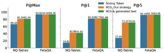
Figure 6. Effect of table representation

Finally, generating text from triples (the RCG&generated text baseline) makes the system much slower (by requiring an inference from the T5 model per triple) without yielding significant accuracy gains. On further analysis, we found that the generated text did not really help with retrieving better content and that in some cases it was erroneous, thus hurting the end-to-end performance.

6.4. RQ4. Microbenchmarks

We consider the impact of different indexing techniques on the first-stage retrieval component (Section 6.4.1) and we demonstrate the impact of the techniques described in (Section 5.2) on runtime in Section 6.4.2.

6.4.1. First-Stage Retrieval Indexing.

The first-stage retrieval index determines the input of the relevance model (Challenge C3), affects the training triples (Challenge C1) and also determines the table representation (Challenge C2). Here, we measure the effect of choosing indexing techniques:

• First Stage (Sparse Index) We index and retrieve triples using the BM25 algorithm (on Elasticsearch) that measures the similarity of question and triple using TF-IDF features (Robertson and Zaragoza, 2009).

• First Stage (Dense Index) This is our first-stage retrieval implementation which uses the Fid Encoder and Faiss index.

• Solo (Sparse Index) We index triples using Elasticsearch, and then construct training data from the sparse Index using the same synthetic questions. We then retrain the relevance model.

Results. Fig. 7 shows the results. The Dense Index outperforms the two sparse indices baselines. The performance gains originate during first-stage retrieval, especially for NQ-Tables with 18 points difference and results in 13 points and 6 points in P@5 and P@1.

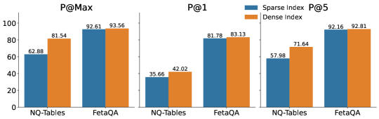
Figure 7. Effect of index type

The Relevance model performs well using the dense index. On FetaQA, the first-stage gap P@MAX is 0.95 points, but the P@1 gap is increased to 1.35 points i.e., the second-stage relevance model benefits more from dense index. The sparse index will retrieve triples based on the overlap with the input question. Because we produce questions from the tables and we use the index to construct training data, this indexing method bias the training dataset towards triples that overlap the most with the input question. The dense index retrieves triples based on semantic similarity that goes beyond the purely syntactic level, resulting in higher performance.

6.4.2. Run-time Performance.

We evaluate the performance of OpenDTR, GTR, Solo, Solo(No student) (where the teacher encoder is used) and Solo(No PQ) (where vectors are added to index without using product quantization). The results on NQ-Tables are summarized in Table 4.

Pipeline	SoLo	SoLo (No Student)	SoLo (No PQ)	OpenDTR Official	GTR Retrain
Encoding Time (# vectors)	1.15 h (41 M )	10.95 h (41 M )	-	0.4 h (0.17M)	-
Building Index Time (Size in GB)	958 s (16 G)	-	960 s (61G)	-	-
Training data collection time	2.4 h	-	-	Manual	Manual
Training time	4.5 h	-	-	4.6h	4.3h
End-to-endPrediction throughput (Index type)	2.6 s/q (Index on disk)	-	-	0.02 s/q (exhaustive search in memory)	-

Table 4. Performance of different systems on NQ-Tables

Results. Table 4 shows the results, with one row for each of the four categories explained above.

$\bullet$ Encoding There are 170k tables in NQ-Tables. Solo generates 41M and OpenDTR only 0.17M, one per table. Although Solo produces more vectors than OpenDTR, it takes less than 3x time (1.15 h vs 0.4 h) to encode the whole table repository. Solo is 9.5x (1.15 h vs 10.95 h) faster than Solo(No student) and this makes our system deployment more practical.

$\bullet$ Building index Solo supports an on-disk index to scale to larger table collections, while OpenDTR uses an in-memory index. It takes only 960 seconds for Solo to index 41M vectors and Solo uses around 1/4 storage size of Solo(No PQ).

$\bullet$ Training data collection Solo automatically collects training data and then it takes 2.4 h to train, while both OpenDTR and GTR-Retrained rely on manual work to collect data. As an example, the NQ-Tables dataset contains 9,534 train questions and 1,067 evaluation questions; collecting these manually is tedious.

$\bullet$ Training runtime All systems were trained on the same synthetic dataset generated by our approach so the training time is similar across approaches.

$\bullet$ Inference throughput Solo achieves subsecond query latencies, permitting interactive querying. Solo’s throughput is lower (2.6 s/q vs 0.02 s/q) than OpenDTR because Solo does not assume vectors fit in memory, thus working in more general scenarios. If we load vectors into memory, the throughput is similar.

The main takeaway message is that the prediction pipeline is slower because of on-disk index search for scalability, which we think can be further optimized, the main gain of Solo is its ability to automatically generate training datasets that lead to high-performance models, as demonstrated in this section.

7. Conclusions

Learned discovery systems offer an attractive way to find data among large table repositories, but they require manual collection of training data, thus limiting their adoption. In response, we introduce a new self-supervised approach to automatically assemble training datasets. We introduce a new table representation method and associated relevance model that makes the system outperform existing approaches. We build a system, Solo, that implements the new strategies and further includes optimizations to reduce encoding and inference time, and storage footprint. Solo outperforms the state of the art baselines. All in all, this work contributes to the growing area of learned data discovery systems.

References

- (1)
- Alabdulmohsin et al. (2022) Ibrahim M Alabdulmohsin, Behnam Neyshabur, and Xiaohua Zhai. 2022. Revisiting neural scaling laws in language and vision. Advances in Neural Information Processing Systems 35 (2022), 22300–22312.
- Allemang et al. (2020) Dean Allemang, James A Hendler, and Fabien Gandon. 2020. Semantic web for the working ontologist. ACM Press.
- Bahri et al. (2021) Yasaman Bahri, Ethan Dyer, Jared Kaplan, Jaehoon Lee, and Utkarsh Sharma. 2021. Explaining neural scaling laws. arXiv preprint arXiv:2102.06701 (2021).
- Blei et al. (2017) David M Blei, Alp Kucukelbir, and Jon D McAuliffe. 2017. Variational inference: A review for statisticians. Journal of the American statistical Association 112, 518 (2017), 859–877.
- Blundell et al. (2015) Charles Blundell, Julien Cornebise, Koray Kavukcuoglu, and Daan Wierstra. 2015. Weight uncertainty in neural network. In International conference on machine learning. PMLR, 1613–1622.
- Borgeaud et al. (2022) Sebastian Borgeaud, Arthur Mensch, Jordan Hoffmann, Trevor Cai, Eliza Rutherford, Katie Millican, George Bm Van Den Driessche, Jean-Baptiste Lespiau, Bogdan Damoc, Aidan Clark, et al. 2022. Improving language models by retrieving from trillions of tokens. In International conference on machine learning. PMLR, 2206–2240.
- Cafarella et al. (2008) Michael J Cafarella, Alon Halevy, Daisy Zhe Wang, Eugene Wu, and Yang Zhang. 2008. Webtables: exploring the power of tables on the web. Proceedings of the VLDB Endowment 1, 1 (2008), 538–549.
- Cappuzzo et al. (2021) Riccardo Cappuzzo, Paolo Papotti, and Saravanan Thirumuruganathan. 2021. EmbDI: Generating Embeddings for Relational Data Integration. (2021).
- Castelo et al. (2021) Sonia Castelo, Rémi Rampin, Aécio Santos, Aline Bessa, Fernando Chirigati, and Juliana Freire. 2021. Auctus: a dataset search engine for data discovery and augmentation. Proceedings of the VLDB Endowment 14, 12 (2021), 2791–2794.
- Chapman et al. (2020) Adriane Chapman, Elena Simperl, Laura Koesten, George Konstantinidis, Luis-Daniel Ibáñez, Emilia Kacprzak, and Paul Groth. 2020. Dataset search: a survey. The VLDB Journal 29, 1 (2020), 251–272.
- Chen et al. (2017) Danqi Chen, Adam Fisch, Jason Weston, and Antoine Bordes. 2017. Reading wikipedia to answer open-domain questions. arXiv preprint arXiv:1704.00051 (2017).
- Chen et al. (2021) Wenhu Chen, Ming-Wei Chang, Eva Schlinger, William Yang Wang, and William W. Cohen. 2021. Open Question Answering over Tables and Text. In International Conference on Learning Representations. https://openreview.net/forum?id=MmCRswl1UYl
- Chen et al. (2020) Zhiyu Chen, Mohamed Trabelsi, Jeff Heflin, Yinan Xu, and Brian D Davison. 2020. Table search using a deep contextualized language model. In Proceedings of the 43rd international ACM SIGIR conference on research and development in information retrieval. 589–598.
- Cherti et al. (2023) Mehdi Cherti, Romain Beaumont, Ross Wightman, Mitchell Wortsman, Gabriel Ilharco, Cade Gordon, Christoph Schuhmann, Ludwig Schmidt, and Jenia Jitsev. 2023. Reproducible scaling laws for contrastive language-image learning. In Proceedings of the IEEE/CVF Conference on Computer Vision and Pattern Recognition. 2818–2829.
- datacityofchicago (2023) datacityofchicago 2023. Chicago data portal. https://data.cityofchicago.org/.
- Dodge et al. (2021) Jesse Dodge, Maarten Sap, Ana Marasović, William Agnew, Gabriel Ilharco, Dirk Groeneveld, Margaret Mitchell, and Matt Gardner. 2021. Documenting large webtext corpora: A case study on the colossal clean crawled corpus. arXiv preprint arXiv:2104.08758 (2021).
- elasticsearch (2023) elasticsearch 2023. Elasticsearch. https://www.elastic.co/.
- Fernandez et al. (2018) Raul Castro Fernandez, Ziawasch Abedjan, Famien Koko, Gina Yuan, Samuel Madden, and Michael Stonebraker. 2018. Aurum: A data discovery system. In 2018 IEEE 34th International Conference on Data Engineering (ICDE). IEEE, 1001–1012.
- Gardent et al. (2017) Claire Gardent, Anastasia Shimorina, Shashi Narayan, and Laura Perez-Beltrachini. 2017. Creating Training Corpora for NLG Micro-Planners. In Proceedings of the 55th Annual Meeting of the Association for Computational Linguistics (Volume 1: Long Papers) (Vancouver, Canada). Association for Computational Linguistics, 179–188. https://doi.org/10.18653/v1/P17-1017
- Gardner et al. (2019) Matt Gardner, Jonathan Berant, Hannaneh Hajishirzi, Alon Talmor, and Sewon Min. 2019. Question Answering is a Format; When is it Useful? arXiv preprint arXiv:1909.11291 (2019).
- Ghorbani et al. (2021) Behrooz Ghorbani, Orhan Firat, Markus Freitag, Ankur Bapna, Maxim Krikun, Xavier Garcia, Ciprian Chelba, and Colin Cherry. 2021. Scaling laws for neural machine translation. arXiv preprint arXiv:2109.07740 (2021).
- Goodfellow et al. (2016) Ian Goodfellow, Yoshua Bengio, and Aaron Courville. 2016. Deep Learning. MIT Press. http://www.deeplearningbook.org.
- Guo et al. (2019) Jiaqi Guo, Zecheng Zhan, Yan Gao, Yan Xiao, Jian-Guang Lou, Ting Liu, and Dongmei Zhang. 2019. Towards complex text-to-sql in cross-domain database with intermediate representation. arXiv preprint arXiv:1905.08205 (2019).
- Halevy et al. (2016) Alon Halevy, Flip Korn, Natalya F Noy, Christopher Olston, Neoklis Polyzotis, Sudip Roy, and Steven Euijong Whang. 2016. Goods: Organizing google’s datasets. In Proceedings of the 2016 International Conference on Management of Data. 795–806.
- Harmouch et al. (2021) Hazar Harmouch, Thorsten Papenbrock, and Felix Naumann. 2021. Relational Header Discovery using Similarity Search in a Table Corpus. In 2021 IEEE 37th International Conference on Data Engineering (ICDE). IEEE, 444–455.
- Herzig et al. (2021) Jonathan Herzig, Thomas Müller, Syrine Krichene, and Julian Martin Eisenschlos. 2021. Open domain question answering over tables via dense retrieval. arXiv preprint arXiv:2103.12011 (2021).
- Herzig et al. (2020) Jonathan Herzig, Paweł Krzysztof Nowak, Thomas Müller, Francesco Piccinno, and Julian Martin Eisenschlos. 2020. TaPas: Weakly supervised table parsing via pre-training. arXiv preprint arXiv:2004.02349 (2020).
- Hinton et al. (2015) Geoffrey Hinton, Oriol Vinyals, and Jeff Dean. 2015. Distilling the knowledge in a neural network. arXiv preprint arXiv:1503.02531 (2015).
- Hristidis et al. (2003) Vagelis Hristidis, Yannis Papakonstantinou, and Luis Gravano. 2003. Efficient IR-style keyword search over relational databases. In Proceedings 2003 VLDB Conference. Elsevier, 850–861.
- Iyyer et al. (2014) Mohit Iyyer, Jordan Boyd-Graber, Leonardo Claudino, Richard Socher, and Hal Daumé III. 2014. A neural network for factoid question answering over paragraphs. In Proceedings of the 2014 conference on empirical methods in natural language processing (EMNLP). 633–644.
- Izacard and Grave (2020a) Gautier Izacard and Edouard Grave. 2020a. Distilling Knowledge from Reader to Retriever for Question Answering. arXiv:2012.04584 [cs.CL]
- Izacard and Grave (2020b) Gautier Izacard and Edouard Grave. 2020b. Leveraging Passage Retrieval with Generative Models for Open Domain Question Answering. arXiv:2007.01282 [cs.CL]
- Jegou et al. (2010) Herve Jegou, Matthijs Douze, and Cordelia Schmid. 2010. Product quantization for nearest neighbor search. IEEE transactions on pattern analysis and machine intelligence 33, 1 (2010), 117–128.
- Johnson et al. (2019) Jeff Johnson, Matthijs Douze, and Hervé Jégou. 2019. Billion-scale similarity search with GPUs. IEEE Transactions on Big Data 7, 3 (2019), 535–547.
- Joshi et al. (2017) Mandar Joshi, Eunsol Choi, Daniel S Weld, and Luke Zettlemoyer. 2017. Triviaqa: A large scale distantly supervised challenge dataset for reading comprehension. arXiv preprint arXiv:1705.03551 (2017).
- Jospin et al. (2022) Laurent Valentin Jospin, Hamid Laga, Farid Boussaid, Wray Buntine, and Mohammed Bennamoun. 2022. Hands-on Bayesian neural networks—A tutorial for deep learning users. IEEE Computational Intelligence Magazine 17, 2 (2022), 29–48.
- Kalinin et al. (2022) Alexandr A Kalinin, Selvam Palanimalai, Junqi Zhu, Wenyi Wu, Nikhil Devraj, Chunchun Ye, Nellie Ponarul, Syed S Husain, and Ivo D Dinov. 2022. SOCRAT: A Dynamic Web Toolbox for Interactive Data Processing, Analysis and Visualization. Information 13, 11 (2022), 547.
- Kaplan et al. (2020) Jared Kaplan, Sam McCandlish, Tom Henighan, Tom B Brown, Benjamin Chess, Rewon Child, Scott Gray, Alec Radford, Jeffrey Wu, and Dario Amodei. 2020. Scaling laws for neural language models. arXiv preprint arXiv:2001.08361 (2020).
- Karpukhin et al. (2020) Vladimir Karpukhin, Barlas Oğuz, Sewon Min, Patrick Lewis, Ledell Wu, Sergey Edunov, Danqi Chen, and Wen-tau Yih. 2020. Dense passage retrieval for open-domain question answering. arXiv preprint arXiv:2004.04906 (2020).
- Katsogiannis-Meimarakis and Koutrika (2023) George Katsogiannis-Meimarakis and Georgia Koutrika. 2023. A survey on deep learning approaches for text-to-SQL. The VLDB Journal (2023), 1–32.
- Keahey et al. (2020) Kate Keahey, Jason Anderson, Zhuo Zhen, Pierre Riteau, Paul Ruth, Dan Stanzione, Mert Cevik, Jacob Colleran, Haryadi S. Gunawi, Cody Hammock, Joe Mambretti, Alexander Barnes, François Halbach, Alex Rocha, and Joe Stubbs. 2020. Lessons Learned from the Chameleon Testbed. In Proceedings of the 2020 USENIX Annual Technical Conference (USENIX ATC ’20). USENIX Association.
- Koch et al. (2023) Maximilian Koch, Mahdi Esmailoghli, Sören Auer, and Ziawasch Abedjan. 2023. Duplicate Table Discovery with Xash. BTW 2023 (2023).
- Kochurov et al. (2018) Max Kochurov, Timur Garipov, Dmitry Podoprikhin, Dmitry Molchanov, Arsenii Ashukha, and Dmitry Vetrov. 2018. Bayesian incremental learning for deep neural networks. arXiv preprint arXiv:1802.07329 (2018).
- Kwiatkowski et al. (2019) Tom Kwiatkowski, Jennimaria Palomaki, Olivia Redfield, Michael Collins, Ankur Parikh, Chris Alberti, Danielle Epstein, Illia Polosukhin, Matthew Kelcey, Jacob Devlin, Kenton Lee, Kristina N. Toutanova, Llion Jones, Ming-Wei Chang, Andrew Dai, Jakob Uszkoreit, Quoc Le, and Slav Petrov. 2019. Natural Questions: a Benchmark for Question Answering Research. Transactions of the Association of Computational Linguistics (2019).
- lambdalabs (2023) lambdalabs 2023. GPU cloud built for deep learning. https://lambdalabs.com/.
- Lewis et al. (2020) Patrick Lewis, Ethan Perez, Aleksandra Piktus, Fabio Petroni, Vladimir Karpukhin, Naman Goyal, Heinrich Küttler, Mike Lewis, Wen-tau Yih, Tim Rocktäschel, et al. 2020. Retrieval-augmented generation for knowledge-intensive nlp tasks. Advances in Neural Information Processing Systems 33 (2020), 9459–9474.
- Liu et al. (2021) Qian Liu, Bei Chen, Jiaqi Guo, Morteza Ziyadi, Zeqi Lin, Weizhu Chen, and Jian-Guang Lou. 2021. Tapex: Table pre-training via learning a neural sql executor. arXiv preprint arXiv:2107.07653 (2021).
- Mialon et al. (2023) Grégoire Mialon, Roberto Dessì, Maria Lomeli, Christoforos Nalmpantis, Ram Pasunuru, Roberta Raileanu, Baptiste Rozière, Timo Schick, Jane Dwivedi-Yu, Asli Celikyilmaz, et al. 2023. Augmented language models: a survey. arXiv preprint arXiv:2302.07842 (2023).
- Min et al. (2019) Sewon Min, Victor Zhong, Luke Zettlemoyer, and Hannaneh Hajishirzi. 2019. Multi-hop reading comprehension through question decomposition and rescoring. arXiv preprint arXiv:1906.02916 (2019).
- Nan et al. (2022) Linyong Nan, Chiachun Hsieh, Ziming Mao, Xi Victoria Lin, Neha Verma, Rui Zhang, Wojciech Kryściński, Nick Schoelkopf, Riley Kong, Xiangru Tang, et al. 2022. FeTaQA: Free-form Table Question Answering. Transactions of the Association for Computational Linguistics 10 (2022), 35–49.
- OpenAI (2023) OpenAI. 2023. GPT-4 Technical Report. https://arxiv.org/abs/2303.08774. (2023).
- openckan (2023) openckan 2023. CKAN, open source data management system. https://ckan.org/.
- Pan et al. (2021) Feifei Pan, Mustafa Canim, Michael Glass, Alfio Gliozzo, and Peter Fox. 2021. CLTR: An End-to-End, Transformer-Based System for Cell Level Table Retrieval and Table Question Answering. arXiv preprint arXiv:2106.04441 (2021).
- Paszke et al. (2017) Adam Paszke, Sam Gross, Soumith Chintala, Gregory Chanan, Edward Yang, Zachary DeVito, Zeming Lin, Alban Desmaison, Luca Antiga, and Adam Lerer. 2017. Automatic differentiation in pytorch. (2017).
- Perez et al. (2020) Ethan Perez, Patrick Lewis, Wen-tau Yih, Kyunghyun Cho, and Douwe Kiela. 2020. Unsupervised question decomposition for question answering. arXiv preprint arXiv:2002.09758 (2020).
- Popescu et al. (2004) Ana-Maria Popescu, Alex Armanasu, Oren Etzioni, David Ko, and Alexander Yates. 2004. Modern natural language interfaces to databases: Composing statistical parsing with semantic tractability. In COLING 2004: Proceedings of the 20th International Conference on Computational Linguistics. 141–147.
- Qiu et al. (2020) Xipeng Qiu, Tianxiang Sun, Yige Xu, Yunfan Shao, Ning Dai, and Xuanjing Huang. 2020. Pre-trained models for natural language processing: A survey. Science China Technological Sciences 63, 10 (2020), 1872–1897.
- Raffel et al. (2019) Colin Raffel, Noam Shazeer, Adam Roberts, Katherine Lee, Sharan Narang, Michael Matena, Yanqi Zhou, Wei Li, and Peter J Liu. 2019. Exploring the limits of transfer learning with a unified text-to-text transformer. arXiv preprint arXiv:1910.10683 (2019).
- Robertson and Zaragoza (2009) Stephen Robertson and Hugo Zaragoza. 2009. The probabilistic relevance framework: BM25 and beyond. Now Publishers Inc.
- Schroff et al. (2015) Florian Schroff, Dmitry Kalenichenko, and James Philbin. 2015. Facenet: A unified embedding for face recognition and clustering. In Proceedings of the IEEE conference on computer vision and pattern recognition. 815–823.
- Shraga et al. (2020) Roee Shraga, Haggai Roitman, Guy Feigenblat, and Mustafa Cannim. 2020. Web table retrieval using multimodal deep learning. In Proceedings of the 43rd International ACM SIGIR Conference on Research and Development in Information Retrieval. 1399–1408.
- Sun et al. (2019) Yibo Sun, Zhao Yan, Duyu Tang, Nan Duan, and Bing Qin. 2019. Content-based table retrieval for web queries. Neurocomputing 349 (2019), 183–189.
- Tobin et al. (2017) Josh Tobin, Rachel Fong, Alex Ray, Jonas Schneider, Wojciech Zaremba, and Pieter Abbeel. 2017. Domain randomization for transferring deep neural networks from simulation to the real world. In 2017 IEEE/RSJ international conference on intelligent robots and systems (IROS). IEEE, 23–30.
- Vaswani et al. (2017) Ashish Vaswani, Noam Shazeer, Niki Parmar, Jakob Uszkoreit, Llion Jones, Aidan N Gomez, Łukasz Kaiser, and Illia Polosukhin. 2017. Attention is all you need. Advances in neural information processing systems 30 (2017).
- Wang et al. (2021) Fei Wang, Kexuan Sun, Muhao Chen, Jay Pujara, and Pedro Szekely. 2021. Retrieving Complex Tables with Multi-Granular Graph Representation Learning. arXiv preprint arXiv:2105.01736 (2021).
- West et al. (2014) Robert West, Evgeniy Gabrilovich, Kevin Murphy, Shaohua Sun, Rahul Gupta, and Dekang Lin. 2014. Knowledge base completion via search-based question answering. In Proceedings of the 23rd international conference on World wide web. 515–526.
- Wilson and Izmailov (2020) Andrew G Wilson and Pavel Izmailov. 2020. Bayesian deep learning and a probabilistic perspective of generalization. Advances in neural information processing systems 33 (2020), 4697–4708.
- Wu et al. (2016) Yonghui Wu, Mike Schuster, Zhifeng Chen, Quoc V Le, Mohammad Norouzi, Wolfgang Macherey, Maxim Krikun, Yuan Cao, Qin Gao, Klaus Macherey, et al. 2016. Google’s neural machine translation system: Bridging the gap between human and machine translation. arXiv preprint arXiv:1609.08144 (2016).
- Yin et al. (2020a) Pengcheng Yin, Graham Neubig, Wen tau Yih, and Sebastian Riedel. 2020a. TaBERT: Pretraining for Joint Understanding of Textual and Tabular Data. In Annual Conference of the Association for Computational Linguistics (ACL).
- Yin et al. (2020b) Pengcheng Yin, Graham Neubig, Wen-tau Yih, and Sebastian Riedel. 2020b. TaBERT: Pretraining for joint understanding of textual and tabular data. arXiv preprint arXiv:2005.08314 (2020).
- Yu et al. (2018) Tao Yu, Rui Zhang, Kai Yang, Michihiro Yasunaga, Dongxu Wang, Zifan Li, James Ma, Irene Li, Qingning Yao, Shanelle Roman, et al. 2018. Spider: A large-scale human-labeled dataset for complex and cross-domain semantic parsing and text-to-sql task. arXiv preprint arXiv:1809.08887 (2018).
- Zhang et al. (2019) Haoyu Zhang, Jingjing Cai, Jianjun Xu, and Ji Wang. 2019. Complex question decomposition for semantic parsing. In Proceedings of the 57th Annual Meeting of the Association for Computational Linguistics. 4477–4486.
- Zhang and Balog (2018) Shuo Zhang and Krisztian Balog. 2018. Ad hoc table retrieval using semantic similarity. In Proceedings of the 2018 world wide web conference. 1553–1562.
- Zhang and Ives (2020) Yi Zhang and Zachary G Ives. 2020. Finding related tables in data lakes for interactive data science. In Proceedings of the 2020 ACM SIGMOD International Conference on Management of Data. 1951–1966.
- Zhao and Fernandez (2022) Zixuan Zhao and Raul Castro Fernandez. 2022. Leva: Boosting Machine Learning Performance with Relational Embedding Data Augmentation. (2022).
- Zhong et al. (2017) Victor Zhong, Caiming Xiong, and Richard Socher. 2017. Seq2SQL: Generating Structured Queries from Natural Language using Reinforcement Learning. CoRR abs/1709.00103 (2017).
- Zhong et al. (2015) ZENG Zhong, Lee Mong Li, and Ling Tok Wang. 2015. Answering Keyword Queries involving Aggregates and Group-Bys in Relational Databases. (2015).