Fractionalization of Majorana-Ising-type quasiparticle excitations
Abstract
We theoretically investigate the spectral properties of a quantum impurity (QI) hosting the here proposed Majorana-Ising-type quasiparticle (MIQ) excitation. It arises from the coupling between a finite topological superconductor (TSC) based on a chain of magnetic adatoms-superconducting hybrid system and an integer large spin flanking the QI. Noteworthy, the spin couples to the QI via the Ising-type exchange interaction. As the Majorana zero-modes (MZMs) at the edges of the TSC chain are overlapped, we counterintuitively find a regime wherein the Ising term modulates the localization of a fractionalized and resonant MZM at the QI site. Interestingly enough, the fermionic nature of this state is revealed as purely of electron tunneling-type and most astonishingly, it has the Andreev conductance completely null in its birth. Therefore, we find that a resonant edge state appears as a zero-mode and discuss it in terms of a poor man’s Majorana[Nature 614, 445 (2023)].
I Introduction
Majorana fermions are peculiar particles equal to their own antiparticles described by real solutions of the Dirac equation[1]. In condensed matter Physics, such fermions rise as quasiparticle excitations usually quoted as Majorana zero-modes (MZMs), which are found attached to the boundaries of topological superconductors (TSCs)[2, 3, 4, 5, 6, 7, 8, 9, 10, 11, 12, 13, 14, 15, 16, 17, 18, 19, 20, 21, 22, 23, 24, 25, 26, 27, 28, 29, 30, 31]. Astonishingly, since the theoretical Kitaev seminal proposal of p-wave superconductivity[32], MZMs are notably coveted due to their attribution as building-blocks for the highly pursued fault-tolerant topological quantum computing. Thereafter, in the last years, such excitations have received astounding focus from both communities working with quantum science and technology.
Interestingly enough, theoretical predictions point out that the fractional zero-bias peak (ZBP) in transport evaluations through quantum dots, which is given by the conductance [2, 3, 4], could have its origin from both the system topological nontrivial regime, where two MZMs emerge spatially far apart at the edges of a TSC[3, 4], as well as in the corresponding trivial, which could exhibit, for instance, Andreev bound states (ABSs)[33, 34]. In this regard, we highlight Ref.[35], which by treating the TSC within the theoretical framework of the Oreg-Lutchyn Hamiltonian[9], allows a detailed and systematic analysis on the formation of MZMs versus ABSs issue. In parallel, effective models[3, 33, 36], despite their simplifications, are used to capture, with a quite good accuracy, the corresponding low-energy Physics encoded by models such as that in Ref.[9] and the Kitaev Hamiltonian[32].
Back to the issue of the topological nontrivial regime, not less important, once an ordinary fermion can be decomposed into two MZMs, is the amplitude in the hallmark of the fractionalization of the quantum of conductance thus giving rise to the concept of fractionalized electronic zero-frequency spectral weight, which indeed reveals, the MZM “half-fermionic” nature[4]. This aforementioned fingerprint is expected to show up in engineered platforms that combine conventional s-wave superconductivity and spin-texture [see Refs.[37, 38, 39] and Fig.1(a)]. As aftermath, the p-wave superconductivity becomes feasible, thus allowing the experimental realization of the spinless Kitaev wire, which is indeed, a TSC in 1D[32, 25, 40, 41, 7, 42, 43, 27]. For such an accomplishment, we highlight two practical recipes based on the Oreg-Lutchyn proposal[9], which have the following ingredients: (i) a semiconducting nanowire, with strong spin-orbit coupling (SOC) and under a magnetic field, should be deposited on top of an s-wave superconductor[29, 30, 31, 25, 40, 41, 44] or (ii) a linear chain of magnetic adatoms with exchange interactions should be hosted by an s-wave superconductor with strong SOC[39, 38, 45, 13, 46, 18, 37, 47, 48, 49, 50, 51]. In both the situations, the s-wave superconductors with singlet Cooper pairing lead to the so-called superconducting proximity effect, which is pivotal to carry forward the superconducting (SC) character into such manufactured Kitaev wires. Thus, the Zeeman field from the previous recipes (i) and (ii), together with the magnified SOC from such quantum materials, establish a synergy that stabilizes the system spin-texture. Consequently, the triplet Cooper pairing for the p-wave superconductivity, as well.
Particularly in the topological nontrivial regime of such setups, these Majorana quasiparticle excitations emerge ideally, i.e., as MZMs decoupled from each other and localized on the boundaries of the TSC. Due to this decoupling from their environment, MZMs are regarded robust against perturbations, once they are topologically protected by the SC gap. Thus, MZMs become promising candidates for a quantum computing free of the decoherence phenomenon[52, 53]. However, perfectly far apart MZMs are hypothetical objects, since they are reliable solely in infinite-size systems and in real experiments, the quantum wires are finite. As a result, these end MZMs within a finite length overlap with each other and inevitably, a fermionic mode with a finite energy emerges instead.
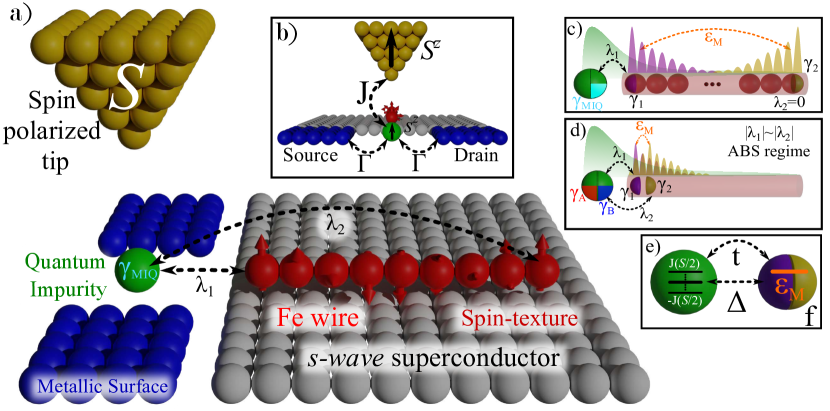
To overcome the aforementioned challenge, in this work, we find as route the fractionalization of ordinary MZMs, in particular, those found at a quantum impurity (QI) site coupled to one edge of a finite TSC in 1D. To this end, we should take into account the Ising exchange interaction between an integer large spin and such a QI. This setup corresponds to Figs.1(a) and (b), and it contains the ordinary MZMs and placed at the edges of a short TSC wire. To better understand our findings, we propose to view the MZMs as sketched in Fig.1(c), where these objects appear symbolized by calottes (half-spheres). We clarify that the employment of such a pictorial representation for the MZMs aims to explain diagrammatically the electron fractionalization into them, as well as the MZM fractionalization itself here observed. These calottes belong to a delocalized sphere cut in half, with each part placed at the TSC edges. This cartoon is very useful and it has the purpose of emulating the nonlocal nature of the fermionic state composed by these MZMs, which are found spatially far apart. To best of our knowledge, the Majorana zero-frequency spectral weight, in particular for a QI coupled to an infinite TSC, is given by the unity when the leaking of the MZM into a quantum dot occurs[4]. This unity corresponds to a calotte, which is a half-electron state that contributes to the conductance as expected[3, 4]. Particularly for a finite TSC, we define as the system sweet spot [see Fig.3b)-I] a special configuration, in which a peculiar Ising exchange interaction allows us to observe a fractionalized MZM quasiparticle excitation at the QI, namely, the called by us as Majorana-Ising-type quasiparticle (MIQ) excitation [Figs.1(a) and (c)]. This quasiparticle excitation can be viewed as the half-calotte within the cartoon representation of the QI state [see also Fig.1(c)]. Such a ratio symbolizes a novel MZM-type excitation in the presence of finite TSCs, in which technically speaking, it is identified by a Majorana zero-frequency spectral weight equals to half. Equivalently, the same amount corresponds to of the entire QI electronic state. In contrast, it leads to as it should be. Interestingly enough, solely in one of the Majorana densities of states (DOSs) of the QI, the MIQ becomes evident as a resonant mode localized at Counterintuitively, the other Majorana DOS of the QI instead of exhibiting a resonant state, reveals a Majorana zero-frequency spectral weight with a valley, but presenting the same magnitude of the resonant Majorana fermion. In this manner, we can safely state that this novel MZM-type quasiparticle excitation, which for simplicity, we just call by MIQ from now on, is then found at the QI. In this situation, we demonstrate that the emergence of such a quasiparticle excitation yields a zero-bias local Andreev conductance entirely null, with only normal electronic contribution to the total conductance.
II The Model
The effective system Hamiltonian that corresponds to the proposed setup presented in Fig.1(a) can be expressed as:
| (1) | |||||
where the operator describes the creation (annihilation) of an electron with momentum , spin- energy for the metallic lead in terms of the single-particle energy and chemical potential while stands for the electrons at the QI site in which represents their energy levels per spin. To connect the QI to the metallic leads and a large spin as well, we should consider the QI-lead coupling which is determined by the QI-lead hopping term and lead DOS in parallel to the Ising-type exchange interaction [Fig.1(b)]. This Ising Hamiltonian involves the components and of the QI and respectively, wherein the latter could be well-represented, within an experimental framework, by a spin-polarized tip [Ref.[54] and Figs.1(a)-(b)]. The emergence of MZMs at the TSC wire edges are accounted for and with as the overlap parameter. Finally, and couple the spin-up channel of the QI to and , respectively [Figs.1(a) and (c)]. Additionally, for the sake of simplicity, we consider that the spin-down degree is decoupled from the TSC and obeys the single impurity Anderson model (SIAM)[55]. Thus, we assume that the spin component of the QI that couples to the Kitaev wire is which is, as can be viewed in Fig.1(a), the same spin direction assumed for the edges of the magnetic chain of adatoms. This means that the spin-flips of the QI electron injected into the TSC and vice-versa are prevented. Therefore, the spin-up degree of the QI is the unique to perceive the TSC. Different spin-textures on the TSC edge where is found[56], which would allow the mixing of the spin degrees of freedom, will be addressed elsewhere and do not belong to the current analysis. Additionally, as we assume the intrinsic Zeeman splitting of the magnetic chain as the largest energy scale, the spin-down has no influence in the phenomenon here reported, once the corresponding electronic occupation is empty. However, even with the present assumption, we are free to demonstrate that both these spin components become influenced by and the TSC that mimics an effective quantum dot tunnel and Andreev-coupled to the QI [Fig.1(e),[57, 58]].
To this end, we call the attention that the Majorana and Ising terms of Eq.(1) should be conveniently rewritten to access the system underlying Physics: (i) the Ising term turns straightforwardly into
| (2) |
due to the standard expansions and with for the QI and large spin, respectively. This means that each spin channel in the QI acquires a multi-level structure split into energies ranging from to As a matter of fact, the TSC alters this feature quite a bit for the channel and (ii) it is imperative to evoke that the MZMs are made by the electron and hole of a regular Dirac fermion delocalized over the TSC edges, which lead to and In this picture, plays the role of the energy level related to the electronic occupation and the QI is indeed hybridized with as mentioned earlier, via the hopping and the superconducting pairing In summary, by considering the parameterization and [Fig.1(a)], we simply find the Kitaev dimer composed by and orbital sites[57, 58]:
| (3) |
Similarly, the spin-up channel of the QI can be also decomposed in MZMs[4], which we label by and i.e.,
| (4) |
Based on Eq.(4), one can compute the Majorana zero-frequency spectral weights for and respectively. These quantities reveal that in the poor man’s Majorana regime ( and )[57, 58] for the Kitaev dimer, that at the QI site, one spectral weight shows a unitary amplitude for a resonant zero-mode, while the other is completely null at zero-energy. It means that an isolated MZM is found at the QI. Analogously, such a feature is also observed in [32, 4]. This results, according to Eq.(3) given by , into two isolated MZMs spatially placed at and orbital sites, namely, and respectively. Although is already nonlocal and split over the TSC edges, it should be understood as an orbital site in the framework of the Kitaev dimer, thus within such a context, is placed there. For the trivial case , the two spectral weights for and attain to unity and then, two resonant zero-modes emerge at the QI site. Thus, Eq.(4) is extremely clarifying, once it points out the possibility of having within the QI, in the presence of and the isolation of the here proposed MIQ. Additionally, as one can notice, the spin down channel always shows the trivial case, due to its decoupling from the TSC. For completeness, the MZMs for we label by and To conclude, we are aware that the QI could also be coupled to the s-wave platform of Fig.1(a) as in Ref.[51] by the term [51, 36] in the limit (infinite superconducting gap standard approximation), where is the s-wave-QI coupling. Nevertheless, differently, we do not consider the on top geometry of Ref.[51] and assumes intrinsic Zeeman splitting of the magnetic chain extremely high, in order to rid off the spin-down component. As a result, we expect that both features suppress and let the exploration to elsewhere when is not found magnified.
III quantum transport and Green’s functions
In this section, our goal is the analytical evaluation of the total conductance through the QI device depicted in Figs.1(a)-(b). As a matter of fact, solely the spin-up channel contributes to the conductance, once the spin-down is energetically inaccessible as previously stated. As our goal is the transport determination around the energy of the MZM, only the bias-energy between source and drain leads (infinite superconducting gap standard approximation) is accounted for in the derivation of our conductance expression below [see Ref.[59] and Appendix B]. In the case of a grounded TSC, symmetric QI-lead couplings independent of being where is the elemental charge and V the corresponding bias-voltage, the crossed Andreev reflection is suppressed and the conductance can be split into[59]
| (5) |
where ET and LAR stand for the electron tunneling and local Andreev reflection processes, respectively, with
| (6) |
wherein and vice-versa, together with
| (7) |
in which the transmittances and are expressed in terms of the frequency-dependent Green’s functions (GFs) of type (details in the Appendix A), due to the presence of the large spin, in which the thermal average should be taken into account. Particularly, these GFs, are indeed the time Fourier transform (with of
| (8) |
where with and
| (9) | ||||
stands for the time-dependent GF following double-brackets Zubarev notation[60], wherein Tr gives the trace over Eq.(1) eigenstates, is the partition function and as the anticommutator.
In practice, the GFs should be determined via the standard equation-of-motion (EOM) approach[61], which in frequency domain, can be summarized as follows
| (10) |
Additionally, Ref.[59] also ensures that the QI normalized DOS obeys the decomposition
| (11) |
As Eq.(11) is bounded to unity, it describes the electronic overall transmittance through the QI decomposed into ET and LAR processes. Specially when it attains to its maximum value at zero energy, i.e., the value gives the electronic zero-frequency spectral weight. In this case, the regular fermionic state of the QI is then made equally by the MZMs and Equivalently, it means that the corresponding normalized DOSs for such quasiparticles localize Majorana states with the same spectral weights and as a result, the QI state is fully built by a pair of resonant MZMs. It gives rise to the conductance Interestingly enough for an isolated ordinary MZM is found at the QI site and the zero-bias conductance is characterized by the hallmark [3, 4]. Such a case corresponds to an ideal infinite superconducting wire. However, there is a regime in which the value is still present for a finite wire and due to the Ising interaction between the large spin and the QI, the observation of the conductance is ensured. This emerges from the novel excitation that we introduce as the MIQ, in particular, by driving the system into the sweet spot for the exchange interaction , namely, In the latter, the index “h” stands for the “half-fermion” special condition of a MZM, which is produced by imposing from where we extract for a given [see Fig.3 b)-I].
Therefore, in order to reveal the aforementioned Physics about the system conductance, we should begin evaluating Eq.(6) for the electron tunneling process. Thus, the GF should be found via the EOM method, which gives
where represents the self-energy correction due to the couplings of the QI with the TSC and the large spin . This also depends on the following defined quantities
| (13) |
| (14) |
and
| (15) |
Concerning the LAR, the conductance of Eq.(7) needs the evaluation of the anomalous GF instead. After performing the EOM approach, it gives rise to
with and
| (17) |
However, if we want to know about the possibility of isolating MZMs in the QI, the DOSs for and should be found in order to examine the emergence of resonant states. To this end, we invert Eq.(4) for and namely, and and we calculate the GFs and Consequently,
| (18) | |||||
where corresponds to respectively. Physically speaking, the sign reversal in can lead to distinct quantum interference phenomena, in particular between those encoded by the normal GFs ( and ) and the corresponding superconducting ( and ). To reveal such interference processes, we need just to find the GFs and to close the evaluation of and By applying the EOM method, we conclude that
and
Naturally, we define the normalized DOSs for and such as
| (21) |
This formula elucidates that when the quantity is fulfilled, it can be recognized as the maximum Majorana quasiparticle transmittance or its corresponding zero-frequency spectral weight.
Henceforward, we focus the attention on the case (grounded SC). We perceive by inspecting Eqs.(LABEL:eq:GFforET) and (LABEL:eq:GFdplusd), that Eq.(11) becomes also Additionally, This in combination with Eqs.(18) and (21) allow us to establish that
| (22) |
Consequently, by taking into account this finding together with Eqs.(5), (6), (7) and (11), we conclude the providential equality as follows
| (23) |
where
stands for the conductance contribution arising from the quasiparticle within the QI.
We highlight that Eq.(23) introduces an alternative perspective concerning the underlying Physics of the conductance in Eq.(5): the ET and LAR quantum transport mechanisms are revealed as the net effect of two Majorana quasiparticle conductances, namely, the corresponding contributions arising from and respectively. In this context, our main findings hold for the constraint fulfilled, thus characterizing the system sweet spot to produce the MIQ. This regime consists of the maximum Majorana quasiparticle transmittance surprisingly, fractionalized and split into and Despite such equipartition, the electronic transmittance is still given by [see Fig.3 b)-I] and according to Eq.(LABEL:eq:GMajorana), it ensures and However, counterintuitively, solely contains a MZM in the common sense, i.e., a resonant state, while shows a dip instead, but with the same magnitude of the peak in This is the reason why we call the contribution by in attention to the emergent MIQ. This is the unique MZM-type resonant state that appears in the system, due to the interplay between the topological superconductivity and the Ising Hamiltonian. In this case, Eqs.(5) and (23) ensure that when the MIQ emerges, exhibits a maximum and shows a minimum, in such a way that only enters into It means that the LAR process is found entirely suppressed within this regime. The complete analysis here summarized will be discussed in the next section.
IV Results
In the entire numerical analysis of Sec.A, we keep constant (grounded SC), () and perform variations in the parameters and Partially for Sec.B, we assume [] from Eq.(1) [Eq.(3)] to analyze the ABSs regime within the framework of the effective model[33]. We should remember that represents the bias- energy between source and drain leads, with the choice in our transport calculations.
IV.1 Majorana-Ising-type quasiparticle (MIQ) excitation
In Fig.2 we present, for the QI of Fig.1, the total conductance of Eq.(5) as a function of the bias-voltage Particularly in Fig.2(a) the ideal case is considered, i.e., the TSC wire is perfectly infinite and the large spin is found turned-off This case is well-known, being characterized by the ZBP in the conductance given by [3, 4]. Interestingly enough, this ZBP in the conductance represents the isolated MZM originally attached to one edge of the TSC wire, which leaks towards the QI site in the form of the MZM The MZM leakage from the TSC edge into the QI is then characterized by the and We will provide extra details concerning this issue in the discussion of the inset a)-I of Fig.3(a). In the other hand, the satellite peaks in Fig.2(a) are the aftermath of the splitting arising from the condition given by Eq.(3) for the poor man’s Majoranas regime of the system[57, 58]. Additionally, we have made explicit via Eq.(5) that the ET and LAR processes compose the total conductance. Thus, such a feature can be viewed in Fig.2(b), where we notice, in particular, for the ZBP conductance that, the ET and LAR split equally. Here we propose that it is still achievable to obtain for a finite TSC wire and to perform also the isolation of a Majorana quasiparticle at the QI site. In our setup, such an excitation rises, in particular, dressed by the Ising interaction. To this end, an integer large spin should be accounted for and be coupled to the QI with a special value in the exchange interaction Thus, by evaluating the amplitude [Eq.(23)] finally becomes restored. However, we will verify that such a configuration corresponds to isolate a peculiar MZM, namely with a resonant peak characterized by the spectral weight [Eq.(21)], while for we have the same amplitude, i.e., but with a dip instead.
Now, we consider the presence of a large spin Figs.2(c) and (d) show the total conductance in the presence of and [see inset b)-I of Fig.3(b)] for a finite TSC with The ZBP conductance in Fig.2(c) is as expected, but the decomposition into ET and LAR channels described in Fig.2(d) reveals a striking result: solely ET survives, while LAR is completely suppressed at zero-bias. Below we will verify that the LAR suppression corresponds to a quasiparticle localization in the DOS for which leads to Thus, according to Eq.(LABEL:eq:GMajorana), such a finite DOS contributes to a conductance where we define the MIQ

In order to understand the emergence of the MIQ, we begin with the trivial case in Fig.3(a): the central panel discriminates the electronic into the corresponding DOSs for and [Eq.(21)] with and This case is regarded as trivial, once we verify that in both the DOSs and resonant states pinned at zero-energy are present. Schematically, the QI fermionic state can be imagined as a sphere formed by two MZMs depicted by two calottes. This is the manner we outline pictorially the two zero-energy resonant states, the so-called MZMs in the DOSs and This sketch can be found in the upper-right inset of Fig.3(a), in which each calotte symbolizes the “half-fermionic” character of the MZM. Equivalently, a calotte occupies the half-volume of the sphere and as it corresponds to a MZM, it can be surely characterized by As aftermath, according to Eqs.(22)-(LABEL:eq:GMajorana), these two MZMs lead to the zero-bias conductance peak Concerning the satellite peaks in the they occur due to the overlap between the MZMs and In the other hand, the inset panel a)-II of Fig.3(a) shows the spin-down channel, which is the one decoupled from the TSC. To analyze it on the same footing as the spin-up channel, we assume artificially and verifies that both the MZMs and which constitute this spin sector of the QI, are then identified exactly by degenerate resonant states. The evaluation of the DOSs for the spin-down sector just employs the GFs for the spin-up sector, but it disregards the superconducting terms. As none of these MZMs overlap with a full superposition of the lineshapes for these MZMs manifests in the profiles of the DOSs and Therefore, satellite peaks do not emerge. Now, let us go back to discuss the spin-up channel. We should pay particular attention to the case depicted in the inset panel a)-I of Fig.3(a), which corresponds to the nonoverlapped situation between and This scenario is the ideal one and it contains the pillars for the conductance behavior of Fig.2(a). Notice that overlaps with leading to satellite peaks in and while is found isolated and localized as a well-defined resonant zero-mode with spectral weight Thereafter, This case is well-known in literature [3, 4] and points out that the MZM contributes to the conductance as a resonant state in contrast to , which shows a gap in around zero-bias. This latter prevents a finite conductance, i.e., Below, we will see that by turning-on the exchange for a given the spectral profiles for the and will exhibit a multi-level structure. Additionally, these densities will be responsible, according to Eq.(LABEL:eq:GMajorana), by a nonquantized in Eq.(23). In the situation of arbitrary the contributions to will not arise from well-defined resonant zero-mode states in and The Majorana fermion localization within the QI as a resonant zero-mode state will only occur for the sweet spot
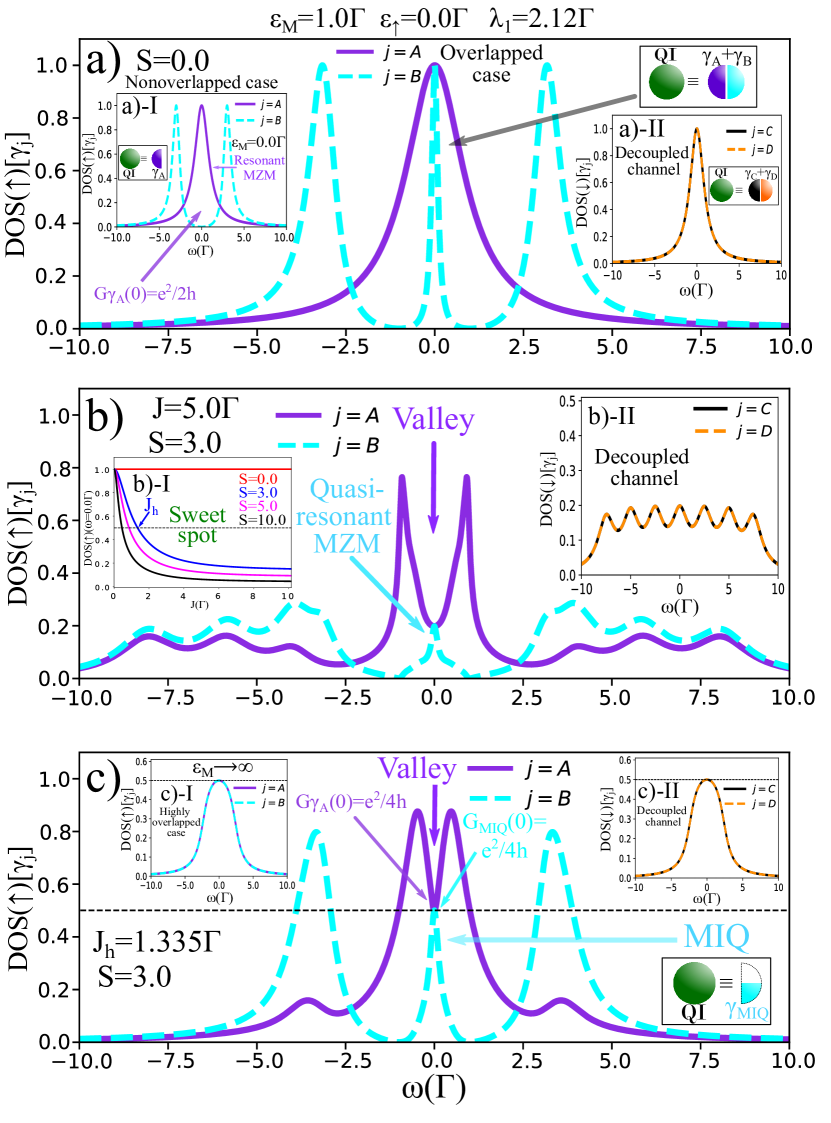
Fig.3(b) treats the presence of a large spin coupled to the QI for As we can notice, the Ising interaction for clearly affects the spectral profiles of and . Basically, it introduces a multi-level structure for the satellite peaks and modifies drastically the MZM localization around the zero-bias. Surprisingly, the presents a valley (dip) at zero-energy and a quasi-resonant MZM rises in As a matter of fact, the latter cannot be considered a well-defined resonant MZM: its spectral weight is not exactly an integer or semi-integer number, and the lineshape broadening does not obey a lorentzian-like form. The lineshapes of such spectral densities are then distinct, but counterintuitively, their zero-bias values coincide, i.e., As the spin-up sector of the QI is the one coupled to the TSC, the spectral profiles in the and do not follow strictly the standard angular momentum theory for the Zeeman splitting [Eq.(2)]. Usually, this theory ensures that for an integer symmetrically displaced levels around the corresponding at should emerge. Here, indeed we observe a mirror-symmetric set with energy bands below and above the zero-bias, respectively, where nearby peculiar spectral structures rise. We reveal that the profiles differ significantly in this range, as aftermath of the nontrivial interplay between the TSC and Ising exchange term. In Figs.4(d)-(f) we will see that the manifestation of this effect lies within a region comprised by cone-like walls spanned by and in the DOSs of the system. Within the cone, the Zeeman splitting becomes unusual and the energy spacing between the levels is simultaneously governed by and Besides, solely the spin-down channel shows standard Zeeman splitting, once it does not perceive the TSC. This can be verified in the inset panel b)-II of Fig.3(b), where the DOSs for and as expected, present the ordinary multi-level structure ensured by Eq.(2). We highlight that upon decreasing the exchange parameter , the restoration of the conductance can be still allowed. Thus, we should remember that such a conductance arises from the fulfillment of the condition Particularly in the inset panel b)-I of Fig.3(b), we show exactly the points where this happens by considering several values of and Particularly for this sweet spot occurs for and its dependence on is revealed as very weak according to our numerical calculations (not shown). It means that still keeps the value while does not exceed very much (). Experimentally speaking, can be tuned by changing the tip-QI vertical distance. Thus for drops from to when Hence, at the sweet spot, if one knows previously the spin of the tip, can be extracted from Fig.3 b)-I or vice-versa.
In Fig.3(c) we present the case that leads to our main finding: a localization of a resonant state at zero-energy in with spectral weight The latter amplitude points out that the ordinary MZM now is fractionalized and the value is not present anymore. This fractionalized MZM, the called MIQ by us, then leads to a conductance as ensured by Eq.(LABEL:eq:GMajorana). The value can be pictorially viewed by the half-calotte found in the lower-right inset of Fig.3(c), which symbolizes the MZM fractionalization within the QI state. Nevertheless, to complete the total conductance the zero-bias value for should coincide, i.e., and as aftermath, as well. Here we emphasize that in a quantum destructive interference manifests and a resonant state does not rise at zero-bias. Moreover, it is capital to clarify the underlying mechanism to produce the MIQ: the key idea is the decrease of thus forcing the merge of the side bands (satellite peaks) of the system towards the zero-energy, where a resonant level is pinned. As a result, this sum of amplitudes for the satellite peaks interferes constructively at zero-energy giving rise to for Further, our findings do not depend on the sign of and in case of a semi-integer large spin, the multi-level structure is even and a zero-energy is absent in the spectrum. In this manner, the MIQ cannot be excited. Concerning the inset panels c)-I and c)-II of Fig.3(c), we verify that for (or ) the DOSs for the Majorana fermions are degenerate. For extremely short TSC wires (), the energy level for the orbital [Eq.(3)] is highly off resonance the QI energy thus making the QI and the TSC to decouple from each other. Thus, the spin-up channel behaves as the corresponding spin-down, which is the one permanently decoupled from the TSC. This implies that the MIQ cannot be seen for very short wires.
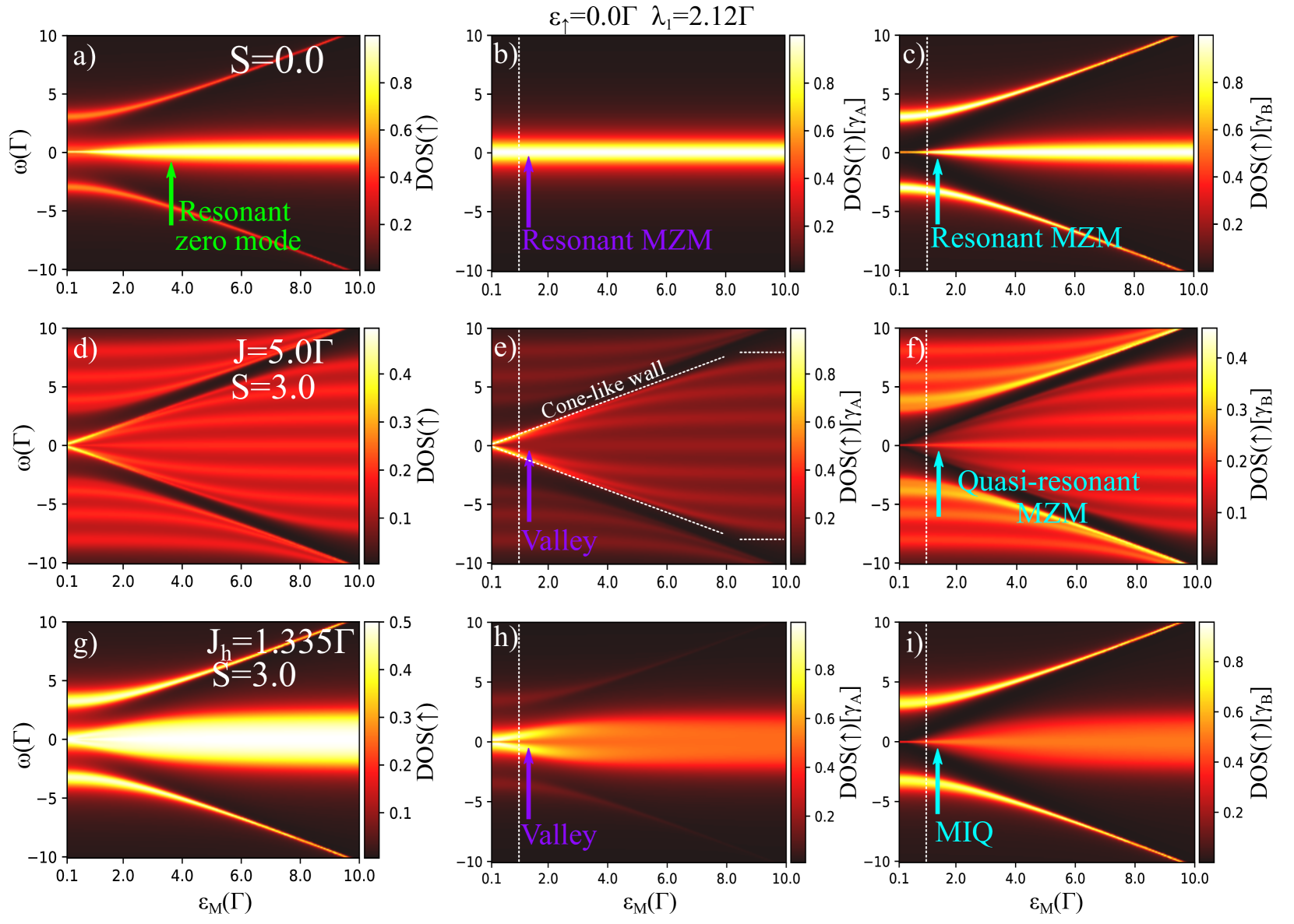
Fig.4 summarizes our findings exhibiting color maps of Eqs.(11) and (21) for the electronic and Majorana DOSs, respectively and spanned by and Panels (a)-(c) describe the case which is characterized by and This corresponds to the trivial regime where two MZMs localize around zero-bias and appear at the QI site. Such a characteristic lies on the zero-bias peaks and appears as horizontal lines in the representation of panels (a)-(c) for any finite value of As we can see, the satellite peaks in (a) arise from (c). By turning-on the Ising interaction with and the spectral profiles of the DOSs acquire distinct patterns: the satellite peaks obey approximately the standard angular momentum theory for the Zeeman splitting, thus exhibiting split side-bands. In this situation, the linear dependence on the exchange parameter is lacking. Besides, the central regions of panels (a)-(c) are converted into the domains delimited by cone-like walls as those found in (d)-(f). While these walls persist up to a threshold in (not marked in the figure), a sophisticated interplay between the TSC and the Ising interaction rules the Physics of the system and allows the possibility of the MIQ existence. Notice that for a multi-level central structure finally becomes resolved. It is worth mentioning that for the line cuts in Fig.4 given by the vertical dashed lines, then correspond to the cases discussed in detail in Fig.3. We would like to mention that the choice corresponds to a strong limit, just to better resolve our findings. However, while stays within the aforementioned cone-like walls, the effect persists. In panels (e) and (f) we notice the rising of the valley and the quasi-resonant MZM spectral structures, respectively upon increasing However, much above the threshold in , the linear spacing in for the Zeeman splitting is restored and this situation is that delimited by the marked horizontal dashed lines. Finally, panels (g)-(i) show the merge of the multi-level structure in the sweet spot leading to the emergence of the MIQ in the Majorana channel while the valley continues in the channel Therefore, within the cone-like walls domain, the sector of Majorana fermions for the QI makes explicit a constructive interference process at zero-bias, while the corresponding in displays a destructive behavior. In this regime, the conductance becomes fully quenched and just contributes to [Fig.2(d)].
IV.2 Poor man’s Majoranas, parity qubit and ABSs regime
In this section, we clarify that the MIQ excitation can be classified as a poor man’s Majorana [57, 58] and to demonstrate such, the analysis of the DOSs for the MZMs of Eq.(3) placed at the Kitaev dimer right edge is performed. To accomplish this goal, we employ pertinent GFs from the Appendix C. Additionally, we discuss the possibility of having a MIQ excitation-based parity qubit for quantum computing purposes[57] and the ABSs regime within the effective model of Eq.(1)[33]. To this end, let us focus again on the left edge of the Kitaev dimer, i.e., the QI. This system part description is found in central panel of Fig.3(a) () and its inset a)-I (), which account for the QI operator where the MZMs and reside [Eq.(4)]. Particularly, these panels show two resonant and single MZMs, respectively, while in Fig.5(a), a resonant MZM appears permanently in the DOS (not normalized, once leads are lacking at this side) for in both the situations, thus describing the MZM placed at the TSC right edge. Such a characteristic is entirely understood within the theoretical framework for the Kitaev dimer described in Ref.[57]. The latter points out that systems based on Eq.(3) for QIs tunnel and Andreev-coupled, which in our case are given by the and orbital sites, could contain the so-called poor man’s Majoranas. These MZMs, in particular, cannot be considered topologically protected as true MZMs, and emerge at the M. Leijnse et al sweet spot[57], when the following set of parameters is obeyed: and This scenario can be observed in the inset panels a)-I of Figs.3 and 5, which reveal resonant MZMs, namely, the poor man’s Majoranas, with one placed at left and the other at right of the Kitaev dimer. This statement holds, since the spectral weights are given by the and for the QI [inset a)-I of Fig.3(a)], while we have and for the Kitaev dimer right edge, as depicted in the inset of Fig.5(a). For the aforementioned case, the nonlocal fermion can be made via the linear combination between the resonant MZMs and localized at right and left of the dimer, respectively[57]. In this manner, the fermion parity, which is given by the electronic occupation of becomes a feasible quantity for quantum computing[57]. For the resonant MZMs and at left depicted in central panel of Fig.3(a) and the corresponding in Fig.5(a), i.e., the situation off the M. Leijnse et al sweet spot with the fragility of these poor man’s Majoranas becomes evident. In such a case, the spectral weights and occur simultaneously at the QI. Thus, according to Ref.[57], the zero-mode dip in the DOS represents the spill of the MZM from the orbital site over the QI, being characterized by the As aftermath, these two resonant MZMs inevitably introduce an ambiguous definition for the nonlocal parity qubit, i.e., it could be or In this way, the parity qubit becomes not well-defined and its employment compromised, as expected, for quantum computing.
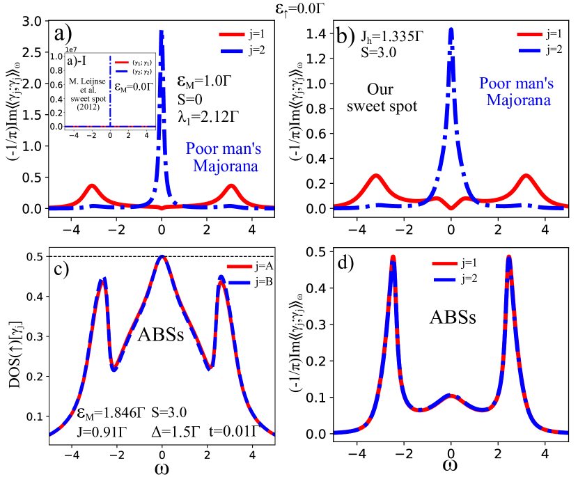
With this in mind, we back to our sweet spot in Fig.3, where the Ising term by considering siphons off the [Fig.3(a)] from resonant profile towards one antiresonant with /2 [Fig.3(c)], while it keeps the [Fig.3(c)] resonant after such a deviation from the value [Fig.3(a)]. As the MZM given by exhibits resonant character and its partner is of antiresonant-type, it means that the QI does not host exactly one MZM. It is an indication that a MZM is spilled over the QI from the orbital site, where the and the resonant still persist, as can be seen in Fig.5(b). Thus, such features reinforce that the MIQ excitation obeys the properties of the poor man’s Majorana[57]. Let us remember that in panels a)-I from Figs.3 and 5, the left and right resonant MZMs were linearly combined to build when However, an extrapolation to for instead, despite being resonant and not, deserves further investigation, once Ref.[57] does not cover such a limit. We let the advances on this particular parity qubit issue to better exploration elsewhere, since they do not belong to the scope of our current research. We call attention that our main findings consist of showing one way of realizing the fractionalization of MZMs, in particular, via the Ising coupling to a QI site.
Still concerning the nature of the fractionalized spectral weight peak given by , we attribute its origin to several modes that added up result into a half-integer contribution.Indeed, each mode, as we know, due to the QI-leads coupling, becomes a band centered at the mode in the absence of the leads. As the separation between the modes (centers of these bands) depends directly on the Ising coupling by decreasing to (our sweet spot), it favors the partial merge of the odd number of bands at zero-energy, where there is an accumulation point. This is naturally imposed by the choice of an integer . Consequently, we find the peak and the dip when we fix in Eq.(22).
In summary, as demonstrated by us, the MIQ excitation (the resonant one) and (the corresponding partner antiresonant) at the system left, together with at right, are poor man’s Majoranas, since they obey their properties of partially protection (not topological) introduced by Ref.[57]. It is worth mentioning that poor man’s Majoranas were recently verified in the experiment of Ref.[58] and in our case, the poor man’s Majoranas observed at the QI show fractionalized characteristic, due to the Ising coupling. At the M. Leijnse et al sweet spot[57], the Ising term plays no role and we still have but with the and a peak in the thus reflecting not fractionalized MZMs. In both the sweet spots, it is capital to note that we have always once we adopt the right side of Eq.(4) as the basis for the quasiparticle excitations of the electron at the QI [Eq.(11)]. This basis is convenient to evaluate the system quantum transport and elucidates if just one MZM (M. Leijnse et al sweet spot) or half of each from the MZM couple of quasiparticle excitations at the QI (our sweet spot), is really contributing to
Figs.5(c) and (d) discuss the ABSs regime, which can be captured by imposing [ ] in Eq.(1) [Eq.(3)], as pointed out by Ref.[33]. It is worth mentioning that such a scenario corresponds to place the MZMs and practically at same TSC edge [see Fig.1(d)], with model parameters marked in Fig.5(c), from where we highlight and Thus, it leads to a conductance which is purely from electron tunneling, but counterintuitively, assisted by Andreev reflection. It means that although through the QI flanked by the leads [Eqs.(7), (LABEL:eq:GFforLAR) and (LABEL:eq:GFdd)], the Kitaev dimer, indeed still admits Andreev reflection, in particular, between the and orbitals given by the terms [Eq.(3),[57]], which then build the quasiparticle electronic state at the QI. As Eqs.(23) and (LABEL:eq:GMajorana) also determine in Fig.5(c), we evaluate then the DOSs [Eq.(21)], which strongly depend only on the GFs and [Eq.(18)], since [Eqs.(LABEL:eq:GFforLAR) and (LABEL:eq:GFdd)] in the ABS regime. By looking at Eqs.(LABEL:eq.Green_dddag) and (LABEL:eq:Green_ddagd) in the Appendix A, we verify that and have a dependence on and which are modulated by the SC pairing and GFs associated to for the Andreev process. Such features establish the Andreev reflection between the QI and while is evaluated at the interface QI-leads. Additionally, we should highlight that similar analysis in observing the ABSs regime, in particular, within the effective model of Eq.(1) but without the Ising term, was already performed by some of us via the analogous Eq.(20) of Ref.[34] and now, we extend it to the current Hamiltonian. As consequences, Fig.5(c) also exhibits the DOSs siphon off to for and which distinct from Figs.5(a) and (b) with are identically resonant. In Fig.5(d), a pair of ABSs manifests too. To conclude, could be reproduced by both the poor man’s Majoranas and ABSs regimes.
V Conclusions
We found that the fractionalization of regular MZMs becomes a feasible task once an integer large spin is exchange coupled to a quantum impurity, in particular when it acts as the new edge of a finite TSC in 1D. A counterintuitive regime arises due to a sweet value for the Ising coupling, which is capable of localizing a fractionalized MZM. We introduce such an excitation as the called Majorana-Ising-type quasiparticle (MIQ). As aftermath, we report the emergence of one MZM with the maximum spectral weight reduced by half and exhibiting resonant character. In contrast, the other MZM mode in the QI does not localize around zero-energy, but shows the same spectral weight of the resonant MZM via an antiresonant profile. Interestingly enough, due to the localization of the MIQ, half of the quantum conductance is made essentially by the normal electronic contribution, while that from the Andreev reflection is totally lacking between the QI and leads. This behavior differs from that observed in perfectly infinite TSC wires, in which one MZM localizes at QI site with maximum spectral weight given by unit and with electronic and Andreev conductances equally split at zero-bias. Therefore, our proposal points out a manner to induce, within a more realistic perspective from an experimental point of view, a quantum state at the edge of a short TSC in 1D. Additionally, our MIQ is demonstrated to be a poor man’s Majorana[57, 58].
VI Acknowledgments
We thank the Brazilian funding agencies CNPq (Grants. Nr. 302887/2020-2, 308410/2018-1, 311980/2021-0, 305668/2018-8 and 308695/2021-6), Coordenação de Aperfeiçoamento de Pessoal de Nível Superior - Brasil (CAPES) – Finance Code 001 and FAPERJ process Nr. 210 355/2018. LSR and IAS acknowledge the support from Icelandic Research Fund (Rannis), projects No. 163082-051 and “Hybrid polaritonics”. LSR thanks ACS and Unesp for their hospitality.
Appendix A Green’s functions for the system left side
As the GFs in the presence of the large spin obey the notation [60], here we make explicit the details in the EOM approach to find the elements of type In what follows, we have
the other two terms are given by
| (27) | |||||
and
| (28) | |||||
And finally the last two GFs associated with the site is
and
With this group of GFs we can determine the complete description of the QI.
Appendix B Quantum transport formalism
Based on the quantum transport Keldysh formalism of Ref.[59], we wrap up here a summary of steps in deriving Eqs.(6), (7) and (11), which assumes the subgap regime (infinite superconducting gap standard approximation) and wide-band limit characterized by an electron-hole symmetry in the QI-leads coupling, which is given by [see the main text below Eq.(1)]. As a result, we have as the total current at the metallic lead the following
| (31) |
where
| (32) |
| (33) |
and
| (34) |
where and refer to the currents for the electron tunneling (ET) and crossed Andreev reflection (CAR) between the QI and the lead but with occupation probabilities of an electron and hole states at lead respectively, where stands for the Fermi distribution at lead and for the electron (hole) quasiparticle. For the local Andreev reflection (LAR) the hole emission is into the same terminal once it depends on
As the total current should conserve, the Kirchhoff’s law holds Additionally, the following assumptions are performed: and the TSC is supposed to be grounded (null chemical potential The former implies in and consequently from Eq.(33), while the latter gives and finally It means that the current only changes the sign from terminal to being the conductance lead independent:
| (35) |
with
| (36) | |||||
and
| (37) | |||||
where we employed the identity again and
| (38) |
with , and .
As when then we deduce Eqs.(6) and (7). To conclude, we should remember that the Keldysh formalism of Ref.[59] also ensures
| (39) |
Appendix C Green’s functions for the system right side
Here we show the GFs for the orbital site and the MZMs and of the Kitaev dimer right side [Eq.(3)]. These quantities are important for Fig.5 and make explicit the poor man’s Majoranas[57, 58] and ABSs[33] regimes in our system. As we know that and we naturally find the GF
| (40) | |||||
where corresponds to , respectively. By applying Eq.(10) for the EOM approach, we obtain
| (41) |
| (42) |
| (43) |
and
| (44) |
with being the self-energy due to the interaction of the site with the QI, which can be expressed in terms of the defined quantities
| (45) |
| (46) |
| (47) |
and
| (48) | |||||
References
- Majorana [1937] E. Majorana, Il Nuovo Cimento (1924-1942) 14, 10.1007/BF02961314 (1937).
- Marra [2022] P. Marra, Journal of Applied Physics 132, 231101 (2022).
- Liu and Baranger [2011] D. E. Liu and H. U. Baranger, Phys. Rev. B 84, 201308 (2011).
- Vernek et al. [2014] E. Vernek, P. H. Penteado, A. C. Seridonio, and J. C. Egues, Phys. Rev. B 89, 165314 (2014).
- Duckheim and Brouwer [2011] M. Duckheim and P. W. Brouwer, Phys. Rev. B 83, 054513 (2011).
- Lutchyn et al. [2010a] R. M. Lutchyn, J. D. Sau, and S. Das Sarma, Phys. Rev. Lett. 105, 077001 (2010a).
- Lesser and Oreg [2022] O. Lesser and Y. Oreg, Journal of Physics D: Applied Physics 55, 164001 (2022).
- Pientka et al. [2014] F. Pientka, L. I. Glazman, and F. von Oppen, Phys. Rev. B 89, 180505 (2014).
- Oreg et al. [2010] Y. Oreg, G. Refael, and F. von Oppen, Phys. Rev. Lett. 105, 177002 (2010).
- Pientka et al. [2013] F. Pientka, L. I. Glazman, and F. von Oppen, Phys. Rev. B 88, 155420 (2013).
- Li et al. [2014] J. Li, H. Chen, I. K. Drozdov, A. Yazdani, B. A. Bernevig, and A. H. MacDonald, Phys. Rev. B 90, 235433 (2014).
- Klinovaja et al. [2013a] J. Klinovaja, P. Stano, A. Yazdani, and D. Loss, Phys. Rev. Lett. 111, 186805 (2013a).
- Nadj-Perge et al. [2013] S. Nadj-Perge, I. K. Drozdov, B. A. Bernevig, and A. Yazdani, Phys. Rev. B 88, 020407 (2013).
- Fu and Kane [2009] L. Fu and C. L. Kane, Phys. Rev. B 79, 161408 (2009).
- Fu and Kane [2008] L. Fu and C. L. Kane, Phys. Rev. Lett. 100, 096407 (2008).
- Vazifeh and Franz [2013] M. M. Vazifeh and M. Franz, Phys. Rev. Lett. 111, 206802 (2013).
- Nakosai et al. [2013] S. Nakosai, Y. Tanaka, and N. Nagaosa, Phys. Rev. B 88, 180503 (2013).
- Braunecker and Simon [2013] B. Braunecker and P. Simon, Phys. Rev. Lett. 111, 147202 (2013).
- Potter and Lee [2012] A. C. Potter and P. A. Lee, Phys. Rev. B 85, 094516 (2012).
- Chung et al. [2011] S. B. Chung, H.-J. Zhang, X.-L. Qi, and S.-C. Zhang, Phys. Rev. B 84, 060510 (2011).
- Beenakker [2015] C. W. J. Beenakker, Rev. Mod. Phys. 87, 1037 (2015).
- Sato and Fujimoto [2016] M. Sato and S. Fujimoto, Journal of the Physical Society of Japan 85, 072001 (2016).
- Sato and Ando [2017] M. Sato and Y. Ando, Reports on Progress in Physics 80, 076501 (2017).
- Haim and Oreg [2019] A. Haim and Y. Oreg, Physics Reports 825, 1 (2019), time-reversal-invariant topological superconductivity in one and two dimensions.
- Alicea [2012] J. Alicea, Reports on Progress in Physics 75, 076501 (2012).
- Beenakker [2013] C. Beenakker, Annual Review of Condensed Matter Physics 4, 113 (2013).
- Karsten Flensberg [2021] A. S. Karsten Flensberg, Felix von Oppen, Nature Reviews Materials 6, 944 (2021).
- Laubscher and Klinovaja [2021] K. Laubscher and J. Klinovaja, Journal of Applied Physics 130, 081101 (2021).
- Deng et al. [2016] M. T. Deng, S. Vaitiekenas, E. B. Hansen, J. Danon, M. Leijnse, K. Flensberg, J. Nygard, P. Krogstrup, and C. M. Marcus, Science 354, 1557 (2016).
- Mourik et al. [2012] V. Mourik, K. Zuo, S. M. Frolov, S. R. Plissard, E. P. A. M. Bakkers, and L. P. Kouwenhoven, Science 336, 1003 (2012).
- Nichele et al. [2017] F. Nichele, A. C. C. Drachmann, A. M. Whiticar, E. C. T. O’Farrell, H. J. Suominen, A. Fornieri, T. Wang, G. C. Gardner, C. Thomas, A. T. Hatke, P. Krogstrup, M. J. Manfra, K. Flensberg, and C. M. Marcus, Phys. Rev. Lett. 119, 136803 (2017).
- Kitaev [2001] A. Y. Kitaev, Physics-Uspekhi 44, 131 (2001).
- Deng et al. [2018] M.-T. Deng, S. Vaitiekėnas, E. Prada, P. San-Jose, J. Nygård, P. Krogstrup, R. Aguado, and C. M. Marcus, Phys. Rev. B 98, 085125 (2018).
- Ricco et al. [2019] L. S. Ricco, M. de Souza, M. S. Figueira, I. A. Shelykh, and A. C. Seridonio, Phys. Rev. B 99, 155159 (2019).
- Liu et al. [2017] C.-X. Liu, J. D. Sau, T. D. Stanescu, and S. Das Sarma, Phys. Rev. B 96, 075161 (2017).
- Ricco et al. [2021] L. S. Ricco, J. E. Sanches, Y. Marques, M. de Souza, M. S. Figueira, I. A. Shelykh, and A. C. Seridonio, Scientific Reports 11, 17310 (2021).
- Nadj-Perge et al. [2014] S. Nadj-Perge, I. K. Drozdov, J. Li, H. Chen, S. Jeon, J. Seo, A. H. MacDonald, B. A. Bernevig, and A. Yazdani, Science 346, 602 (2014).
- Ruby et al. [2015] M. Ruby, F. Pientka, Y. Peng, F. von Oppen, B. W. Heinrich, and K. J. Franke, Phys. Rev. Lett. 115, 197204 (2015).
- Pawlak et al. [2016] R. Pawlak, M. Kisiel, J. Klinovaja, T. Meier, S. Kawai, T. Glatzel, D. Loss, and E. Meyer, npj Quantum Information 2, 10.1038/npjqi.2016.35 (2016).
- Elliott and Franz [2015] S. R. Elliott and M. Franz, Rev. Mod. Phys. 87, 137 (2015).
- Aguado [2017] R. Aguado, LA RIVISTA DEL NUOVO CIMENTO 40, 523 (2017).
- Leijnse and Flensberg [2012a] M. Leijnse and K. Flensberg, Semiconductor Science and Technology 27, 124003 (2012a).
- Stanescu and Tewari [2013] T. D. Stanescu and S. Tewari, Journal of Physics: Condensed Matter 25, 233201 (2013).
- Lutchyn et al. [2010b] R. M. Lutchyn, J. D. Sau, and S. Das Sarma, Phys. Rev. Lett. 105, 077001 (2010b).
- Choy et al. [2011] T.-P. Choy, J. M. Edge, A. R. Akhmerov, and C. W. J. Beenakker, Phys. Rev. B 84, 195442 (2011).
- Klinovaja et al. [2013b] J. Klinovaja, P. Stano, A. Yazdani, and D. Loss, Phys. Rev. Lett. 111, 186805 (2013b).
- Jeon et al. [2017] S. Jeon, Y. Xie, J. Li, Z. Wang, B. A. Bernevig, and A. Yazdani, Science 358, 772 (2017).
- Marra and Nitta [2019] P. Marra and M. Nitta, Phys. Rev. B 100, 220502 (2019).
- Pawlak et al. [2019] R. Pawlak, S. Hoffman, J. Klinovaja, D. Loss, and E. Meyer, Progress in Particle and Nuclear Physics 107, 1 (2019).
- Jack et al. [2021] B. Jack, Y. Xie, and A. Yazdani, Nature Reviews Physics 3, 2522 (2021).
- Górski et al. [2018] G. Górski, J. Baranski, I. Weymann, and T. Domanski, Scientific Reports 8, 15717 (2018).
- Nayak et al. [2008] C. Nayak, S. H. Simon, A. Stern, M. Freedman, and S. Das Sarma, Rev. Mod. Phys. 80, 1083 (2008).
- Sarma et al. [2015] S. D. Sarma, M. Freedman, and C. Nayak, npj Quantum Information 1, 2056 (2015).
- Wiesendanger [2009] R. Wiesendanger, Rev. Mod. Phys. 81, 1495 (2009).
- Anderson [1961] P. W. Anderson, Phys. Rev. 124, 41 (1961).
- Prada et al. [2017] E. Prada, R. Aguado, and P. San-Jose, Phys. Rev. B 96, 085418 (2017).
- Leijnse and Flensberg [2012b] M. Leijnse and K. Flensberg, Phys. Rev. B 86, 134528 (2012b).
- Dvir et al. [2023] T. Dvir, G. Wang, N. van Loo, C.-X. Liu, G. P. Mazur, A. Bordin, S. L. D. ten Haaf, S. L. D. ten Haaf, J.-Y. Wang, D. van Driel, F. Zatelli, X. Li, F. K. Malinowski, S. Gazibegovic, G. Badawy, E. P. A. M. Bakkers, M. Wimmer, and L. P. Kouwenhoven, Nature 614, 445 (2023).
- Máthé et al. [2022] L. Máthé, D. Sticlet, and L. P. Zârbo, Phys. Rev. B 105, 155409 (2022).
- Zubarev [1960] D. N. Zubarev, Soviet Physics Uspekhi 3, 320 (1960).
- Bruus and Flensberg [2012] H. Bruus and K. Flensberg, (Oxford: Oxford University Press) (2012).