22email: francisco.aragon@ua.es 33institutetext: Boris S. Mordukhovich 44institutetext: Department of Mathematics, Wayne State University, Detroit, Michigan 48202, USA
44email: boris@math.wayne.edu 55institutetext: Pedro Pérez-Aros 66institutetext: Instituto de Ciencias de la Ingeniería, Universidad de O’Higgins, Rancagua, Chile
66email: pedro.perez@uoh.com
Coderivative-Based Semi-Newton Method
in Nonsmooth Difference Programming
††thanks: Research of the first author was partially supported by the Ministry of Science, Innovation and Universities of Spain and the European Regional Development Fund (ERDF) of the European Commission, Grant PGC2018-097960-B-C22, and by the Generalitat Valenciana, grant AICO/2021/165. Research of the second author was partially supported by the USA National Science Foundation under grants DMS-1808978 and DMS-2204519, by the Australian Research Council under Discovery Project DP-190100555, and by the Project 111 of China under grant D21024. Research of the third author was partially supported by grants: Fondecyt Regular 1190110 and Fondecyt Regular 1200283.
Abstract
This paper addresses the study of a new class of nonsmooth optimization problems, where the objective is represented as a difference of two generally nonconvex functions. We propose and develop a novel Newton-type algorithm to solving such problems, which is based on the coderivative generated second-order subdifferential (generalized Hessian) and employs advanced tools of variational analysis. Well-posedness properties of the proposed algorithm are derived under fairly general requirements, while constructive convergence rates are established by using additional assumptions including the Kurdyka–Łojasiewicz condition. We provide applications of the main algorithm to solving a general class of nonsmooth nonconvex problems of structured optimization that encompasses, in particular, optimization problems with explicit constraints. Finally, applications and numerical experiments are given for solving practical problems that arise in biochemical models, constrained quadratic programming, etc., where advantages of our algorithms are demonstrated in comparison with some known techniques and results.
Keywords:
Nonsmooth difference programming generalized Newton methods global convergence convergence rates variational analysis generalized differentiationMSC:
49J53, 90C15, 9J521 Introduction
The primary mathematical model considered in this paper is described by
| (1) |
where is of class (i.e., the collection of -smooth functions with locally Lipschitzian derivatives), and where is a locally Lipschitzian and prox-regular function; see below. Although (1) is a problem of unconstrained optimization, it will be shown below that a large class of constrained optimization problems can be reduced to this form. In what follows, we label the optimization class in (1) as problems of difference programming.
The difference form (1) reminds us of problems of DC difference of convex programming, which have been intensively studied in optimization with a variety of practical applications; see, e.g., Aragon2020 ; Artacho2019 ; AragonArtacho2018 ; Oliveira_2020 ; hiriart ; Toh ; Tao1997 ; Tao1998 ; Tao1986 and the references therein. However, we are not familiar with a systematic study of the class of difference programming problems considered in this paper.
Our main goal here is to develop an efficient numerical algorithm to solve the class of difference programs (1) with subsequent applications to nonsmooth and nonconvex problems of particular structures, problems with geometric constraints, etc. Furthermore, the efficiency of the proposed algorithm and its modifications is demonstrated by solving some practical models for which we conduct numerical experiments and compare the obtained results with previously known developments and computations by using other algorithms. The proposed algorithm is of a regularized damped Newton type with a novel choice of directions in the iterative scheme providing a global convergence of iterates to a stationary point of the cost function. At the first order, the novelty of our algorithm, in comparison with, e.g., the most popular DCA algorithm by Tao et al. Tao1997 ; Tao1998 ; Tao1986 and its boosted developments by Aragón-Artacho et al.Aragon2020 ; Artacho2019 ; AragonArtacho2018 ; MR4078808 in DC programming, is that instead of a convex subgradient of in (1), we now use a limiting subgradient of . No second-order information on is used in what follows. Concerning the other function in (1), which is nonsmooth of the second-order, our algorithm replaces the classical Hessian matrix by the generalized Hessian/second-order subdifferential of in the sense of Mordukhovich m92 . The latter construction, which is defined as the coderivative of the limiting subdifferential has been well recognized in variational analysis and optimization due its comprehensive calculus and explicit evaluations for broad classes of extended-real-valued functions arising in applications. We refer the reader to, e.g., chhm ; dsy ; Helmut ; hmn ; hos ; hr ; 2020arXiv200910551D ; MR3823783 ; MR2191744 ; mr ; os ; yy and the bibliographies therein for more details. Note also that the aforementioned generalized Hessian has already been used in differently designed algorithms of the Newton type to solve optimization-related problems of different nonsmooth structures in comparison with (1); see Helmut ; 2020arXiv200910551D ; jogo ; 2021arXiv210902093D ; BorisEbrahim . Having in mind the discussions above, we label the main algorithm developed in this paper as the regularized coderivative-based damped semi-Newton method (abbr. RCSN).
The rest of the paper is organized as follows. Section 2 recalls constructions and statements from variational analysis and generalized differentiation, which are broadly used in the formulations and proofs of the major results. Besides well-known facts, we present here some new notions and further elaborations.
In Section 3, we design our main RCSN algorithm, discuss each of its steps, and establish various results on its performance depending on imposed assumptions whose role and importance are illustrated by examples. Furthermore, Section 4 employs the Kurdyka-Łojasiewicz (KL) property of the cost function to establish quantitative convergence rates of the RCSN algorithm depending on the exponent in the KL inequality.
Section 5 addresses the class of (nonconvex) problems of structured optimization with the cost functions given in the form , where is a twice continuously differentiable function with a Lipschitzian Hessian (i.e., of class ), while is an extended-real-valued prox-bounded function. By using the forward-backward envelope MR3845278 and the associated Asplund function asplund , we reduce this class of structured optimization problems to the difference form (1) and then employ the machinery of RCSN to solving problems of this type. As a particular case of RCSN, we design and justify here a new projected-like Newton algorithm to solve optimization problems with geometric constraints given by general closed sets.
Section 6 is devoted to implementations of the designed algorithms and numerical experiments in two different problems arising in practical modeling. Although these problems can be treated after some transformations by DCA-like algorithms, we demonstrate in this section numerical advantages of the newly designed algorithms over the known developments in both smooth and nonsmooth settings. The concluding Section 7 summarizes the major achievements of the paper and discusses some directions of our future research.
2 Tools of Variational Analysis and Generalized Differentiation
Throughout the entire paper, we deal with finite-dimensional Euclidean spaces and use the standard notation and terminology of variational analysis and generalized differentiation; see, e.g., MR3823783 ; MR1491362 , where the reader can find the majority of the results presented in this section. Recall that stands for the closed ball centered at with radius and that .
Given a set-valued mapping , its graph is the set , while the (Painlevé–Kuratowski) outer limit of at is defined by
| (2) |
For a nonempty set , the (Fréchet) regular normal cone and (Mordukhovich) basic/limiting normal cone at are defined, respectively, by
| (3) | ||||
where “” means that with . We use the convention if . The indicator function of is equal to 0 if and to otherwise.
For a lower semicontinuous (l.s.c.) function , its domain and epigraph are given by and respectively. The regular and basic subdifferentials of at are defined by
| (4) | ||||
via the corresponding normal cones (3) to the epigraph. The function is said to be lower/subdifferentially regular at if .
Given further a set-valued mapping/multifunction , the regular and basic coderivatives of at are defined for all via the corresponding normal cones (3) to the graph of , i.e.,
| (5) | ||||
where is omitted if is single-valued at . When is single-valued and locally Lipschitzian around , the basic coderivative has the following representation via the basic subdifferential of the scalarization
| (6) |
Recall that a set-valued mapping is strongly metrically subregular at if there exist such that
| (7) |
It is well-known that this property of is equivalent to the calmness property of the inverse mapping at . In what follows, we use the calmness property of single-valued mappings at meaning that there exist positive numbers and such that
| (8) |
The infimum of all in (8) is called the exact calmness bound of at and is denoted it by . On the other hand, a multifunction is strongly metrically regular around if its inverse admits a single-valued and Lipschitz continuous localization around this point.
Along with the (first-order) basic subdifferential in (4), we consider the second-order subdifferential/generalized Hessian of at relative to defined by
| (9) |
and denoted by when is a singleton. If is twice continuously differentiable (-smooth) around , then .
Next we introduce an extension of the notion of positive-definiteness for multifunctions, where the the corresponding constant may not be positive.
Definition 1
Let and . Then is -lower-definite if
| (10) |
Remark 1
We can easily check the following:
(i) For any symmetric matrix with the smallest eigenvalue , the function is -lower-definite.
(ii) If a function is strongly convex with modulus , (i.e., is convex), it follows from (MR3823783, , Corollary 5.9) that is -lower-definite for all .
(iii) If are and -lower-definite, then the sum is -lower-definite.
Recall next that a function is prox-regular at for if it is l.s.c. around and there exist and such that
| (11) |
whenever with and . If this holds for all , is said to be prox-regular at .
Remark 2
The class of prox-regular functions has been well-recognized in modern variational analysis. It is worth mentioning that if is a locally Lipschitzian function around , then the following properties of are equivalent: (i) prox-regularity at , (ii) lower- at , and (iii) primal-lower-nice at ; see, e.g., (MR2101873, , Corollary 3.12) for more details.
Given a function and , the upper directional derivative of at with respect to is defined by
| (12) |
The following proposition establishes various properties of prox-regular functions used below. We denote the convex hull of a set by “co”.
Proposition 1
Let be locally Lipschitzian around and prox-regular at this point. Then is lower regular at , , and for any we have the representations
| (13) |
Proof
First we fix an arbitrary subgradient and deduce from (11) applied to and that
Passing to the limit as tells us that
which means that and thus shows that is lower regular at . By the Lipschitz continuity of around and the convexity of the set , we have that , where denotes the (Clarke) generalized gradient. It follows from that , which implies therefore that .
Pick , and find by the prox-regularity of at for that there exists such that
if is small enough. This yields for all and thus verifies the inequality “” in the first representation of (13).
To prove the opposite inequality therein, take such that
Employing the mean value theorem from (MR3823783, , Corollary 4.12)) gives us
It follows from the Lipschitz continuity of that is bounded, and so we can assume that . Therefore,
which verifies (13) and completes the proof of the proposition.
Next we define the notion of stationary points for problem (1) the finding of which is the goal of our algorithms.
Definition 2
Remark 3
The stationarity notion , expressed via the limiting subdiffential, is known as the Mordukhovich-stationarity. Since no other stationary points are considered in this paper, we skip “M” in what follows. Observe from the subdifferential sum rule in our setting that is a stationary point in (1) if and only if . Thus every stationary point is a critical point in the sense that . By Proposition 1, the latter can be equivalently described in terms of the generalized gradient and also via the symmetric subdifferential MR3823783 of at defined by
| (14) |
which possesses the plus-minus symmetry . When both and are convex, the classical DC algorithm Tao1986 ; Tao1997 and its BDCA variant MR4078808 can be applied for solving problem (1). Although these algorithms only converge to critical points, they can be easily combined as in Aragon2020 with a basic derivative-free optimization scheme to converge to d-stationary points, which satisfy (or, equivalently, for all ; see (Aragon2020, , Proposition 1)). In the DC setting, every local minimizer of problem (1) is a d-stationary point (Toland1979, , Theorem 3), a property which is stronger than the notion of stationarity in Definition 2.
To proceed, recall that a mapping defined on an open set is semismooth at if it is locally Lipschitzian around , directionally differentiable at this point, and the limit
exists for all , where , and where is the set on which is differentiable; see MR1955649 ; MR3289054 for more details. We say that a function is semismoothly differentiable at if is -smooth around and its gradient mapping is semismooth at this point.
Recall further that a function is prox-bounded if there exists such that for some , where is the Moreau envelope of with parameter defined by
| (15) |
The number is called the threshold of prox-boundedness of . The corresponding proximal mapping is the multifunction given by
| (16) |
Next we observe that that the Moreau envelope can be represented as a DC function. For any function , consider its Fenchel conjugate
and for any and , define the Asplund function
| (17) |
which is inspired by Asplund’s study of metric projections in asplund . The following proposition presents the precise formulation of the aforementioned statement and reveals some remarkable properties of the Asplund function (17).
Proposition 2
Let be a prox-bounded function with threshold . Then for every , we have the representation
| (18) |
where the Asplund function is convex and Lipschitz continuous on . Furthermore, for any the following subdifferential evaluations hold:
| (19) | ||||
| (20) |
Moreover, if is such that , then the vector belongs to . If in addition is of class on , then the function is prox-regular at any point .
Proof
Representation (18) easily follows from definitions of the Moreau envelope and Asplund function. Due to the second equality in (17), the Asplund function is convex on . It is also Lipschitz continuous due its finite-valuedness on , which is induced by this property of the Moreau envelope. The subdifferential evaluations in (19) and (MR1491362, , Example 10.32) and the subdifferential sum rule in (MR3823783, , Proposition 1.30)) tell us that and for any .
Take further with and show that . Indeed, it follows from (19) that
The Lipschitz continuity and convexity of implies that
| (21) |
by (MR2191744, , Theorem 3.57), which allows us to deduce from (20) and (21) that
This verifies the inclusion as claimed.
Observe finally that the function is the composition of the convex function and the mapping , which ensures by (MR2069350, , Proposition 2.3) its prox-regularity at any point .
The following remark discusses a useful representation of the basic subdifferential of the function and other functions of this type.
Remark 4
It is worth mentioning that the subdifferential can be expressed via the set as follows:
| (22) |
We refer to (MR1491362, , Theorem 10.31) for more details. Note that we do not need to take the convex hull on the right-hand side of (22) as in the case of the generalized gradient of locally Lipschitzian functions.
Finally, recall the definitions of the convergence rates used in the paper.
Definition 3
Let be a sequence in converging to as . The convergence rate is said to be:
(i) R-linear if there exist , and such that
(ii) Q-linear if there exists such that
(iii) Q-superlinear if it is Q-linear for all , i.e., if
(iv) Q-quadratic if we have
3 Regularized Coderivative-Based Damped Semi-Newton Method in Nonsmooth Difference Programming
The goal of this section is to justify the well-posedness and good performance of the novel algorithm RCSN under appropriate and fairly general assumptions. In the following remark, we discuss the difference between the choice of subgradients and hence of directions in RCSN and DC algorithms.
Our main RCSN algorithm to find stationary points of nonsmooth problems (1) of difference programming is labeled below as Algorithm 1.
| (23) |
Remark 5
Observe that Step 2 of Algorithm 1 selects , which is equivalent to choosing in the basic subdifferential of at . Under our assumptions, the set can be considerably smaller than ; see the proof of Proposition 1 and also Remark 4 above. Therefore, Step 2 differs from those in DC algorithms, which choose subgradients in . The purpose of our development is to find a stationary point instead of a (classical) critical point for problem (1). In some applications, Algorithm 1 would not be implementable if the user only has access to subgradients contained in instead of . In such cases, a natural alternative to Algorithm 1 would be a scheme replacing in Step 2 by with . Under the setting of our convergence results, the modified algorithm would find a critical point for problem (1), which is not guaranteed to be stationary.
The above discussions are illustrated by the following example.
Example 1
Consider problem (1) with and . If an algorithm similar to Algorithm 1 was run by using as the initial point but choosing with (instead of ), it would stop at the first iteration and return , which is a critical point, but not a stationary one. On the other hand, for any we get , and so Algorithm 1 will continue iterating until it converges to one of the two stationary points and , which is guaranteed by our main convergence result; see Theorem 3.1 below.
The next lemma shows that Algorithm 1 is well-defined by proving the existence of a direction satisfying (23) in Step 3 for sufficiently large regularization parameters .
Lemma 1
Let be the objective function in problem (1) with and being locally Lipschitz around and prox-regular at this point. Further, assume that is -lower-definite for some and consider a nonzero subgradient . Then for any and any , there exists a nonzero direction satisfying the inclusion
| (24) |
Moreover, any nonzero direction from (24) obeys the conditions:
(i) .
(ii) Whenever , there exists such that
Proof
Consider the function for which we clearly have that , where denotes the identity mapping. This shows by Remark 1 that is -lower-definite, and thus it is -lower-definite as well. Since and , it follows from (2021arXiv210902093D, , Proposition 3.1) (which requires to be on , but actually only around is needed) that there exists a nonzero direction such that . This readily verifies (24), which yields in turn the second inequality in (i) due to Definition 1. On the other hand, we have by Proposition 1 the following:
| (25) |
where in the last estimate is a consequence of the second inequality in (i).
Remark 6
Under the -lower-definiteness of , Lemma 1 guarantees the existence of a direction satisfying both conditions in (23) for all . When is unknown, it is still possible to implement Step 3 of the algorithm as follows. Choose first any initial value of , then compute a direction satisfying the inclusion in (23) and continue with Step 4 if the descent condition in (23) holds. Otherwise, increase the value of and repeat the process until the descent condition is satisfied.
The next example demonstrates that the prox-regularity of is not a superfluous assumption in Lemma 1. Namely, without it the direction used in Step 3 of Algorithm 1 can even be an ascent direction.
Example 2
Consider the least squares problem given by
with and . Denote and . If we pick , the function is not prox-regular at because it is not lower regular at ; see Proposition 1. Indeed, , while
Therefore, although is -lower-definite, the assumptions of Lemma 1 are not satisfied. Due to the representation
the choice of yields . For any , inclusion (24) gives us . This is an ascent direction for the objective function at due to
which illustrates that the prox-regularity is an essential assumption in Lemma 1.
Algorithm 1 either stops at a stationary point, or produces an infinite sequence of iterates. The convergence properties of the iterative sequence of our algorithm are obtained below in the main theorem of this section. Prior to the theorem, we derive yet another lemma, which establishes the following descent property for the difference of a function and a prox-regular one.
Lemma 2
Let , where is of class around , and where is continuous around and prox-regular at this point. Then for every , there exist positive numbers and such that
whenever and .
Proof
Pick any and deduce from the imposed prox-regularity and continuity of that there exist and such that
| (26) |
and all . It follows from the property of by (MR3289054, , Lemma A.11) that there exist positive numbers and such that
| (27) |
Summing up the inequalities in (26) and (27) and defining and , we get that
for all and all . This completes the proof.
Now we are ready to establish the aforementioned theorem about the performance of Algorithm 1.
Theorem 3.1
Let be the objective function of problem (1) given by with . Pick an initial point and suppose that the sublevel set is closed. Assume also that:
(a) The function is around every and the second-order subdifferential is -lower-definite for all with some .
(b) The function is locally Lipschitzian and prox-regular on .
Then Algorithm 1 either stops at a stationary point, or produces sequences , , , , and such that:
(i) The sequence monotonically decreases and converges.
(ii) If as is any bounded subsequence of , then ,
In particular, the boundedness of the entire sequence ensures that the set of accumulation points of is a nonempty, closed, and connected.
(iii) If as , then is a stationary point of problem (1) with the property .
(iv) If has an isolated accumulation point , then the entire sequence converges to as , where is a stationary point of (1).
Proof
If Algorithm 1 stops after a finite number of iterations, then it clearly returns a stationary point. Otherwise, it produces an infinite sequence . By Step 5 of Algorithm 1 and Lemma 1, we have that for all , which proves assertion (i) and also shows that .
To proceed, suppose that has a bounded subsequence (otherwise there is nothing to prove) and split the rest of the proof into the five claims.
Claim 1: The sequence , associated with as and produced by Algorithm 1, is bounded from below.
Indeed, otherwise consider a subsequence of such that as . Since is bounded, we can assume that converges to some point . By Lemma 1, we have that
| (28) |
which yields by the Cauchy–Schwarz inequality the estimate
| (29) |
Since is locally Lipschitzian and , we suppose without loss of generality that converges to some as . It follows from (29) that is bounded, and therefore along a subsequence. Since , we can assume that for all , and hence Step 5 of Algorithm 1 ensures the inequality
| (30) |
Lemma 2 gives us a constant such that
| (31) |
for all sufficiently large. Combining (30), (31), and (28) tells us that
for large . Since by (28), we get that for such , which contradicts the choice of and thus verifies this claim.
Claim 2: We have the series convergence , , and .
To justify this, deduce from Step 5 of Algorithm 1 and Lemma 1 that
It follows from Claim 1 that for all , which yields . On the other hand, we have that , and again Claim 1 ensures that . To proceed further, let and use the Lipschitz continuity of on the compact set . Employing the subdifferential condition from (MR3823783, , Theorem 4.15) together with the coderivative scalarization in (6), we get by the standard compactness argument the existence of such that
for all and all . Therefore, it follows from the inclusion that we have
| (32) |
Using finally the triangle inequality and the estimate leads us to the series convergence as stated in Claim 2.
Claim 3: If the sequence is bounded, then the set of its accumulation points is nonempty, closed and connected.
Applying Claim 2 to the sequence , we have the Ostrowski condition . Then, the conclusion follows from (Ostrowski1966, , Theorem 28.1).
Claim 4: If as , then is a stationary point of (1) being such that .
By Claim 2, we have that the sequence with as . The closedness of the basic subgradient set ensures that . The second assertion of the claim follows from the continuity of at .
Claim 5: If has an isolated accumulation point , then the entire sequence of converges to as , and is a stationary point of (1). Indeed, consider any subsequence . By Claim 4, is a stationary point of (1), and it follows from Claim 2 that . Then we deduce from by (MR1955649, , Proposition 8.3.10) that as , which completes the proof of theorem.
Remark 7
Regarding Theorem 3.1, observe the following:
(i) If , is of class , and , then the results of Theorem 3.1 can be found in 2021arXiv210902093D .
(ii) If , we can choose the regularization parameter and (a varying) in (23) for some to verify that assertions (i) and (iii) of Theorem 3.1 still hold. Indeed, if converges to some , then is bounded by the Lipschitz continuity of . Hence the sequence converges to . Otherwise, there exists and a subsequence of whose norms are bounded from below by . Using the same argumentation as in the proof of Theorem 3.1 with , we arrive at the contradiction with being an accumulation point of of .
When the objective function is coercive and its stationary points are isolated, Algorithm 1 converges to a stationary point because Theorem 3.1(iii) ensures that the set of accumulation points is connected. This property enables us to prove the convergence in some settings when even there exist nonisolated accumulation points; see the two examples below.
Example 3
Consider the function given by
This function is clearly -smooth and coercive. For any starting point , the level set is bounded, and hence there exists a number such that the functions and satisfy the assumptions of Theorem 3.1. Observe furthermore that is a DC function because it is -smooth; see, e.g., Oliveira_2020 ; hiriart . However, it is not possible to write its DC decomposition with and for , since there exists no scalar such that the function is convex on the entire real line.
It is easy to see that the stationary points of are described by . Moreover, if Algorithm 1 generates an iterative sequence starting from , then the accumulation points form by Theorem 3.1(ii) a nonempty, closed, and connected set . If , the sequence converges to . If contains any point of the form , then it is an isolated point, and Theorem 3.1(iv) tells us that the entire sequence converges to that point, and consequently we have .
Example 4
Consider the function given by
We can easily check that the function is coercive and satisfies the assumptions of Theorem 3.1 with , , and . For this function, the points in the set are critical but not stationary. Moreover, the points in the set give the global minima to the objective function . Therefore, Algorithm 1 leads us to global minimizers of starting from any initial point.
The following theorem establishes convergence rates of the iterative sequences in Algorithm 1 under some additional assumptions.
Theorem 3.2
Suppose in addition to the assumptions of Theorem 3.1, that has an accumulation point such that the subgradient mapping is strongly metrically subregular at . Then the entire sequence converges to with the Q-linear convergence rate for and the R-linear convergence rate for and . If furthermore, , , , , , is semismoothly differentiable at , is of class around , and , then the rate of convergence of all the sequences above is at least Q-superlinear.
Proof
We split the proof of the theorem into the following two claims.
Claim 1: The rate of convergence of
is at least Q-linear, while both sequences and converge at least R-linearly.
Observe first that it follows from the imposed strong metric subregularity of that is an isolated accumulation point, and so as by Theorem 3.1(iii). Further, we get from (7) that there exists such that
| (33) |
since as by Theorem 3.1(ii). Using (32) and the triangle inequality gives us such that for sufficiently large . Lemma 2 yields then the cost function increment estimate
| (34) |
By Step 5 of Algorithm 1 and Lemma 1, we get that for large . Remembering that , we deduce from Theorem 3.1(ii) the existence of such that
| (35) |
whenever large enough. Therefore, applying (2021arXiv210902093D, , Lemma 7.2) to the sequences , , and with the positive constants , , and , we verify the claimed result.
Claim 2: Assuming that , , is semismoothly differentiable at , is of class around , and , we have that the rate of convergence for all the above sequences is at least Q-superlinear.
Suppose without loss of generality that is differentiable at any . It follows from the coderivative scalarization (6) and the basic subdifferential sum rule in (MR3823783, , Theorem 2.19) valid under the imposed assumptions that
| (36) |
This yields the existence of such that
| (37) |
Moreover, the -lower-definiteness of and the Cauchy–Schwarz inequality imply that
Combining now the semismoothness of at with the conditions and brings us to the estimates
Then we have and deduce therefore from (MR1955649, , Proposition 8.3.18) and Lemma 1(i) that
| (38) |
It follows from (38) that if for large . Applying (MR1955649, , Proposition 8.3.14) yields the -superlinear convergence of to as .
Remark 8
The property of strong metric subregularity of subgradient mappings, which is a central assumption of Theorem 3.2, has been well investigated in variational analysis, characterized via second-order growth and coderivative type conditions, and applied to optimization-related problems; see, e.g., ag ; dmn ; MR3823783 and the references therein.
The next theorem establishes the -superlinear and -quadratic convergence of the sequences generated by Algorithm 1 provided that: (i.e., is -strongly positive-definite), for all (no regularization is used), is semismoothly differentiable at the cluster point , and the function can be expressed as the pointwise maximum of finitely many affine functions at , i.e., when there exist and such that
| (40) |
Theorem 3.3
In addition to the assumptions of Theorem 3.1, suppose that , , , , and for all . Suppose also that the sequence generated by Algorithm 1 has an accumulation point at which is semismoothly differentiable and can be represented in form (40). Then we have the convergence , , , and as with at least -superlinear rate. If in addition is of class around , then the rate of convergence is at least quadratic.
Proof
Observe that by (40) and (MR2191744, , Proposition 1.113) we have the inclusion
| (41) |
for all near . The rest of the proof is split into the five claims below.
Claim 1: The sequence converges to as .
Observe that is an isolated accumulation point. Indeed, suppose on the contrary that there is a sequence of accumulation points of such that as with for all . Since each is accumulation point of , they are stationary points of . The -smoothness of ensures that as , and so (41) yields
for large . Since there are finitely many of in (40), we get that when is sufficiently large. Further, it follows from (MR3823783, , Theorem 5.16) that the gradient mapping is strongly locally maximal monotone around , i.e., there exist positive numbers and such that
Putting and in the above inequality tells us that for large , which is a contradiction. Applying finally Theorem 3.1(iv), we complete the proof of this claim.
Claim 2: The sequence converges to as at least -superlinearly.
As , we have by Theorem 3.1(ii) that , and so it follows from (41) that
there exists such that , and
for all sufficiently large. Define the auxiliary function by
| (42) |
and observe that is around and semismoothly differentiable at this point. We have the equalities
| (43) |
for large . It follows from that the mapping is -lower-definite. Using (36) and (37) with the replacement of by and taking (43) into account ensures the existence of satisfying the estimate
The triangle inequality and the semismoothness of at yield
which tells us that . Then it follows from(MR1955649, , Proposition 8.3.18) and Lemma 1(i) above that
| (44) |
whenever is sufficiently large. Applying finally (MR1955649, , Proposition 8.3.14) verifies the claimed -superlinear convergence of to .
Claim 3: The gradient mapping of from (42) is strongly metrically regular around and hence strongly metrically subregular at this point.
Using the -lower-definiteness of and the pointbased coderivative characterization of strong local maximal monotonicity given in (MR3823783, , Theorem 5.16), we verify this property for
around . Then (MR3823783, , Corollary 5.15) ensures that is strongly metrically regular around .
Claim 4: The sequences , , and converge at least Q-superlinearly to , , and , respectively.
It follows from the estimates in (39), with the replacement of by and with taking into account that
and due to (43), that there exist constants such that
provided that is sufficiently large. Recalling that for large completes the proof of the claim.
Claim 5: If is of class around , then the rate of convergence of the sequences above is at least quadratic.
It is easy to see that the assumed property of yields this property of around . Using estimate
(44), we deduce this claim from the quadratic convergence of the classical Newton method; see, e.g., (Aragon2019, , Theorem 5.18) and (MR3289054, , Theorem 2.15). This therefore completes the proof of the theorem.
Remark 9
Concerning Theorem 3.3, observe the following:
(i) It is important to emphasize that the performance of Algorithm 1 revealed in Theorem 3.3 is mainly due to the usage of the basic subdifferential of the function in contrast to that of , which is calculated as
| (45) |
by (MR2191744, , Theorem 3.46). We can see from the proof of Theorem 3.3 that it fails if the evaluation of in (41) is replaced by the one of in (45).
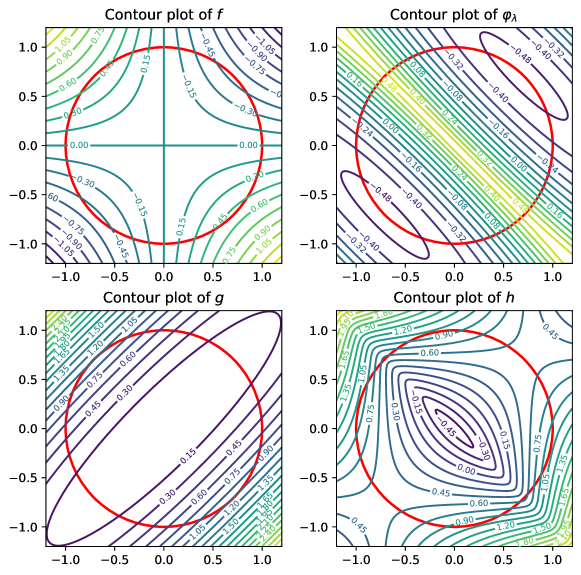
(ii) The main assumptions of Theorem 3.3 do not imply the smoothness of at stationary points. For instance, consider the nonconvex function defined as in Example 4 but letting now . The function satisfies the assumptions of Theorem 3.3 at any of its stationary points , but is not differentiable at ; see Figure 2.
4 Convergence Rates under the Kurdyka–Łojasiewicz Property
In this section, we verify the global convergence of Algorithm 1 and establish convergence rates in the general setting of Theorem 3.1 without additional assumptions of Theorems 3.2 and 3.3 while supposing instead that the cost function satisfies the Kurdyka–Łojasiewicz property. Recall that the Kurdyka–Łojasiewicz property holds for at if there exist and a continuous concave function with such that is -smooth on with the strictly positive derivative and that
| (46) |
for all with , where stands for the distance function of a set .
The first theorem of this section establishes the global convergence of iterative sequence generated by Algorithm 1 to a stationary point of (1).
Theorem 4.1
Proof
If Algorithm 1 stops after a finite number of iterations, there is nothing to prove. Due to the decreasing property of from Theorem 3.1(i), we can assume that for all . Let be the accumulation point of where satisfies the Kurdyka–Łojasiewicz inequality (46), which by Theorem 3.1 is a stationary point of problem (1). Since is continuous, we have that . Taking the constant and the function from (46) and remembering that is of class around , suppose without loss of generality that is Lipschitz continuous on with modulus . Let be such that and that
| (47) |
for all , where , , and are the constants of Algorithm 1. The rest of the proof is split into the following three steps.
Claim 1: Let be such that . Then we have the estimate
| (48) |
Indeed, it follows from (6), (23), and (MR3823783, , Theorem 1.22) that
| (49) |
Then using Step 5 of Algorithm 1, Lemma 1, the Kurdyka–Łojasiewicz inequality (46), the concavity of , and estimate (49) gives us
which therefore verifies the claimed inequality (48).
Claim 2: For every , we have the inclusion .
Suppose on the contrary that there exists with and define . Since for the estimate in (48) is satisfied, we get by using (47) that
which contradicts our assumption and thus verifies this claim.
Claim 3: We have that , and consequently the sequence converges to as .
It follows from Claim 1 and Claim 2 that (48) holds for all . Thus
which therefore completes the proof of the theorem.
The next theorem establishes convergence rates for iterative sequence in Algorithm 1 provided that the function in (46) is selected in a special way. Since the proof while using Theorem 4.1, is similar to the corresponding one from (MR4078808, , Theorem 4.9) in a different setting, it is omitted.
Theorem 4.2
In addition to the assumptions of Theorem 4.1, suppose that the Kurdyka–Łojasiewicz property (46) holds at the accumulation point with for some and . The following assertions hold:
(i) If , then the sequence converges in a finite number of steps.
(ii) If , then the sequence converges at least linearly.
(iii) If , then there exist and such that
Remark 10
Together with our main Algorithm 1, we can consider its modification with the replacement of by . In this case, the most appropriate version of the Kurdyka–Łojasiewicz inequality (46), ensuring the fulfillment the corresponding versions of Theorem 4.1 and 4.2, is the one
expressed in terms of the symmetric subdifferential from (14). Note that the latter is surely satisfied where the symmetric subdifferential is replaced by the generalized gradient , which is the convex hull of .
5 Applications to Structured Constrained Optimization
In this section, we present implementations and specifications of our main RCSN Algorithm 1 for two structured classes of optimization problems. The first class contains functions represented as sums of two nonconvex functions one of which is smooth, while the other is extended-real-valued. The second class concerns minimization of smooth functions over closed constraint sets.
5.1 Minimization of Structured Sums
Here we consider the following class of structured optimization problems:
| (50) |
where is of class with the -Lipschitzian gradient, and where is an extended-real-valued prox-bounded function with the threshold . When both functions and are convex, problems of type (50) have been largely studied under the name of “convex composite optimization” emphasizing the fact that and are of completely different structures. In our case, we do not impose any convexity of and prefer to label (50) as minimization of structured sums to avoid any confusions with optimization of function compositions, which are typically used in major models of variational analysis and constrained optimization; see, e.g., MR1491362 .
In contrast to the original class of unconstrained problems of difference programming (1), the structured sum optimization form (50) covers optimization problems with constraints given by . Nevertheless, we show in what follows that the general class of problem (50) can be reduced under the assumptions imposed above to the difference form (1) satisfying the conditions for the required performance of Algorithm 1.
This is done by using an extended notion of envelopes introduced by Patrinos and Bemporad in Patrinos2013 , which is now commonly referred as the forward-backward envelope; see, e.g., MR3845278 .
Definition 4
Given and , the forward-backward envelope (FBE) of the function with the parameter is defined by
| (51) |
Remembering the constructions of the Moreau envelope (15) and the Asplund function (17) allows us to represent for every as:
| (52) |
Remark 11
It is not difficult to show that whenever is -Lipschitz on and , the optimal values in problems (1) and (51) are the same
| (53) |
Indeed, the inequality “” in (53) follows directly from the definition of . The reverse inequality in (53) is obtained by
Moreover, (53) does not hold if is not Lipschitz continuous on . Indeed, consider and . Then we have while , which yields , and so (53) fails.
The next theorem shows that FBE (51) can be written as the difference of a function and a Lipschitzian prox-regular function. Furthermore, it establishes relationships between minimizers and critical points of and .
Theorem 5.1
Let , where is of class and where is prox-bounded with threshold . Then for any , we have the inclusion
| (54) |
Furthermore, the following assertions are satisfied:
(i) If is a stationary point of , then provided that the matrix is nonsingular.
(ii) The FBE (51) can be written as , where is of class , and where is locally Lipschitzian and prox-regular on . Moreover, is -lower-definite for all with .
(iii) If for a closed set , then , where denotes the generally set-valued projection operator onto . In this case, inclusion (54) holds as an equality.
(iv) If both and are convex, we have that , where and are of class and hence prox-regular on , and that
| (55) |
provided that is nonsingular at any stationary point of .
Proof
Observe that inclusion (54) follows directly by applying the basic subdifferential sum and chain rules from (MR3823783, , Theorem 2.19 and Corollary 4.6), respectively, the first representation of in (52) with taking into account the results of Lemma 2. Now we pick any stationary point of the FBE and then deduce from and (54) that
which readily implies that and thus verifies (i). Assertion (ii) follows directly from Proposition 2 and the smoothness of .
To prove (iii), we need to verify the reverse inclusion “” in (19), for which it suffices to show that the inclusion yields . On the contrary, if , then there exist and such that with . By definition of the projection, we get the equalities
which contradict the strict convexity of and thus verifies (iii).
The first statement in (iv) follows from the differentiability of and of the Moreau envelope by (MR1491362, , Theorem 2.26). Further, the inclusion “” in (55) is a consequence of (i). To justify the reverse inclusion in (55), observe that any satisfying is a global minimizer of the convex function , and so . The differentiability of and (54) (which holds as an equality in this case) tells us that , and thus (55) holds. This completes the proof of the theorem.
Remark 12
Based on Theorem 5.1(ii), it is not hard to show that the FBE function can be represented as a difference of convex functions. Indeed, since is a locally Lipschitzian and prox-regular function, we have by (MR2101873, , Corollary 3.12) that is a lower- function, and hence by (MR1491362, , Theorem 10.33), it is locally a DC function. Similarly, being a function is a DC function, so the difference is also a DC function. However, it is difficult to determine for numerical purposes what is an appropriate representation of as a difference of convex functions. Moreover, such a representation of the objective in terms of convex functions may generate some theoretical and algorithmic challenges as demonstrated below in Example 5.
5.2 Nonconvex Optimization with Geometric Constraints
This subsection addresses the following problem of constrained optimization with explicit geometric constraints given by:
| (56) |
where is of class , and where is an arbitrary closed set. Due to the lack of convexity, most of the available algorithms in the literature are not able to directly handle this problem. Nevertheless, Theorem 5.1 provides an effective machinery allowing us to reduce (56) to an optimization problem that can be solved by using our developments. Indeed, define and observe that is prox-regular with threshold . In this setting, FBE (51) reduces to the formula
Furthermore, it follows from Theorem 5.1(iii) that
Based on Theorem 5.1, we deduce from Algorithm 1 with its following version to solve the constrained problem (56).
To the best of our knowledge, Algorithm 2 is new even for the case of convex constraint sets . All the results obtained for Algorithm 1 in Sections 3 and 4 can be specified for Algorithm 2 to solve problem (56). For brevity, we present just the following direct consequence of Theorem 3.1.
Corollary 1
Considering problem (56), suppose that is of class , that is closed, and that . Pick an initial point and a parameter . Then Algorithm 2 either stops at a point such that , or generates infinite sequences , , , , and satisfying the assertions:
(i) The sequence monotonically decreases and converges.
(ii) If is a bounded subsequence of , then and
If, in particular, the entire sequence is bounded, then the set of its accumulation points is nonempty, closed, and connected.
(iii) If as , then and the equality holds.
(iv) If the sequence has an isolated accumulation point , then it converges to as , and we have .
The next example illustrates our approach to solve (56) via Algorithm 2 in contrast to algorithms of the DC type.
Example 5
Consider the minimization of a quadratic function over a closed (possibly nonconvex) set :
| (57) |
where is a symmetric matrix, and where . In this setting, FBE (51) can be written as with
| (58) |
Our method does not require a DC decomposition of the objective function . Indeed the function in (58) is generally nonconvex. Specifically, consider , , and being the unit sphere centered at the origin. Then in (58) is strongly convex for any , while therein is not convex whenever . More precisely, in this case we have
This tells us, in particular, that
and thus is not convex regardless of the value of ; see Figure 3.
6 Further Applications and Numerical Experiments
In this section, we demonstrate the performance of Algorithm 1 and Algorithm 2 in two different problems. The first problem is smooth and arises from the study of system biochemical reactions. It can be successfully tackled with DCA-like algorithms, but they require to solve subproblems whose solutions cannot be analytically computed and are thus time-consuming. This is in contrast to Algorithm 1, which only requires solving the linear equation (23) at each iteration. The second problem is nonsmooth and consists of minimizing a quadratic function under both convex and nonconvex constraints. Employing FBE (51) and Theorem 5.1, these two problems can be attacked by using DCA, BDCA, and Algorithm 2.
Both Algorithms 1 and 2 have complete freedom in the choice of the initial value of the stepsizes in Step 4, as long as they are bounded from below by a positive constant , while the choice of totally determines the performance of the algorithms. On the one hand, a small value would permit the stepsize to get easily accepted in Step 5, but it would imply little progress in the iteration and (likely) in the reduction of the objective function, probably making it more prone to stagnate at local minima. On the other hand, we would expect a large value to ameliorate these issues, while it could result in a significant waste of time in the linesearch Steps 5-7 of both algorithms.
Therefore, it makes sense to consider a choice which sets the trial stepsize depending on the stepsize accepted in the previous iteration, perhaps increasing it if no reduction of the stepsize was needed. This technique was introduced in (MR4078808, , Section 5) under the name of Self-adaptive trial stepsize, and it was shown there that this accelerates the performance of BDCA in practice. A similar idea is behind the so-called two-way backtracking linesearch, which was recently proposed in Truong2021 for the gradient descent method, showing good numerical results on deep neural networks. In contrast to BDCA, our theoretical results require to be strictly positive, so the technique should be slightly adapted as shown in Algorithm 3. Similarly to MR4078808 , we adopt a conservative rule of only increasing the trial stepsize when two consecutive trial stepsizes were accepted without decreasing them.
The codes in the first subsection below were written and ran in MATLAB version R2021b, while for the second subsection we used Python 3.8. The tests were ran on a desktop of Intel Core i7-4770 CPU 3.40GHz with 32GB RAM, under Windows 10 (64-bit).
6.1 Smooth DC Models in Biochemistry
Here we consider the problem motivating the development of BDCA in AragonArtacho2018 , which consists of finding a steady state of a dynamical equation arising in the modeling of biochemical reaction networks. We ran our experiments on the same 14 biochemical reaction network models tested in AragonArtacho2018 ; MR4078808 . The problem can be modeled as finding a zero of the function
where denote the forward and reverse stoichiometric matrices, respectively, where is the componentwise logarithm of the kinetic parameters, where is the componentwise exponential function, and where stands for the horizontal concatenation operator. Finding a zero of is equivalent to minimizing the function , which can be expressed as a difference of the convex functions
| (59) |
where the functions and are given by
In addition, it is also possible to write
and so can be decomposed as the difference of the functions
| (60) |
with being convex. Therefore, is -lower definite, and minimizing can be tackled with Algorithm 1 by choosing for some fixed . As shown in AragonArtacho2018 , the function is real analytic and thus satisfies the Kurdyka–Łojasiewicz assumption of Theorem 4.2, but as observed in (AragonArtacho2018, , Remark 5), a linear convergence rate cannot be guaranteed.
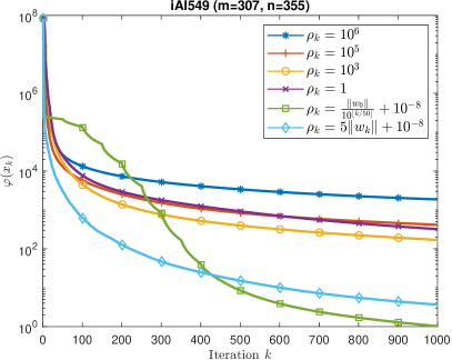
Our first task in the conducted experiments was to decide how to set the parameters and . We compared the strategy of taking equal to some fixed value for all , setting a decreasing sequence bounded from below by , and choosing for some constant . In spite of Remark 7(ii), was added in the last strategy to guarantee both Theorem 3.1(ii) and Theorem 4.2. We took and a constant , which worked well in all the models. We tried several options for the decreasing strategy, of which a good choice seemed to be , where denotes the floor function (i.e., the parameter was initially set to and then divided by every 50 iterations). The best option was this decreasing strategy, as can be observed in the two models in Figure 4, and this was the choice for our subsequent tests.
Experiment 1
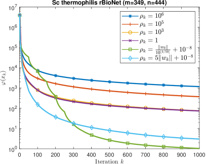
For finding a steady state of each of the 14 biochemical models, we compared the performance of Algorithm 1 and BDCA with self-adaptive strategy, which was the fastest method tested in MR4078808 (on average, 6.7 times faster than DCA). For each model, 5 kinetic parameters were randomly chosen with coordinates uniformly distributed in , and 5 random starting points with random coordinates in were picked. BDCA was ran using the same parameters as in MR4078808 , while we took for Algorithm 1.
We considered two strategies for setting the trial stepsize in Step 4 of Algorithm 1: constantly initially set to 50, and self-adaptive strategy (Algorithm 3) with and . For each model and each random instance, we computed 500 iterations of BDCA with self-adaptive strategy and then ran Algorithm 1 until the same value of the target function was reached. As in AragonArtacho2018 , the BDCA subproblems were solved by using the function fminunc with optimoptions('fminunc', 'Algorithm', 'trust-region', 'GradObj', 'on', 'Hessian', 'on', 'Display', 'off', 'TolFun', 1e-8, 'TolX', 1e-8).
The results are summarized in Figure 5, where we plot the ratios of the running times between BDCA with self-adaptive stepsize and Algorithm 1 with constant trial stepsize against Algorithm 1 with self-adaptive stepsize. On average, Algorithm 1 with self-adaptive strategy was times faster than BDCA, and was times faster than Algorithm 1 with constant strategy. The lowest ratio for the times of self-adaptive Algorithm 1 and BDCA was . Algorithm 1 with self-adaptive stepsize was only once (out of the 70 instances) slightly slower (a ratio of 0.98) than with the constant strategy.
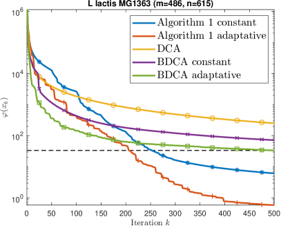
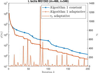
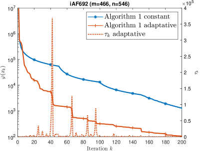
In Figure 6, we plot the values of the objective function for each algorithm and also include for comparison the results for DCA and BDCA without self-adaptive strategy. The self-adaptive strategy also accelerates the performance of Algorithm 1. We can observe in Figure 7 that there is a correspondence between the drops in the objective value and large increases of the stepsizes (in a similar way to what was shown for BDCA in (MR4078808, , Fig. 12)).

6.2 Solving Constrained Quadratic Optimization Models
This subsection contains numerical experiments to solve problems of constrained quadratic optimization formalized by
| (61) |
where is a symmetric matrix (not necessarily positive-semidefinite), , and are nonempty, closed, and convex sets.
When (i.e., ), this problem is referred as the trust-region subproblem. If is positive-semidefinite, then (61) is a problem of convex quadratic programming. Even when is not positive-semidefinite, Tao and An Tao1998 showed that this particular instance of problem (61) could be efficiently addressed with the DCA algorithm by using the following DC decomposition:
| (62) |
where . However, this type of decomposition would not be suitable for problem (61) when is not convex.
As shown in Subsection 5.2, problem (61) for can be reformulated by using FBE (51) to be tackled with Algorithm 2 with . Although the decomposition in (58) may not be suitable for DCA when is not positive-definite, it can be regularized by adding to both and with . Such a regularization would guarantee the convexity of the resulting functions and given by
| (63) | ||||
| (64) |
The function in (62) is not smooth, but the function in (63) is. Then it is possible to apply BDCA MR4078808 to formulation (63)–(64) in order to accelerate the convergence of DCA. Note that it would also be possible to do it with (62) if the or balls were used; see Artacho2019 for more details.
Let us describe two numerical experiments to solve problem (61).
Experiment 2
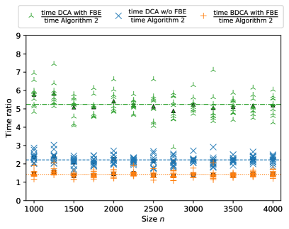
Consider (61) with and replicate the hardest setting in Tao1998 , which was originally considered in More1983 . Specifically, in this experiment we generated potentially difficult cases by setting for some diagonal matrix and orthogonal matrix with , . The components of were random numbers uniformly distributed in , while the elements in the diagonal of were random numbers in . We took for some vector whose elements were random numbers uniformly distributed in except for the component corresponding to the smallest element of , which was set to . The radius was randomly chosen in the interval , where if and otherwise.
For each , we generated 10 random instances, took for each instance a random starting point in , and ran from it the four algorithms described above: DCA applied to formulation (62) (without FBE), DCA and BDCA applied to (63)–(64), and Algorithm 2. We took as the parameter for FBE (both for DCA and Algorithm 2). The regularization parameter was chosen as for DCA with FBE and for BDCA, as should be strongly convex. Both Algorithm 2 and BDCA were ran with the self-adaptive trial stepsize for the backtracking step introduced in MR4078808 with parameters and , and with . For the shake of fairness, we did not compute function values for the runs of DCA at each iteration, since it is not required by the algorithm. Instead, we used for both versions of DCA the stopping criterion from Tao1998 that , where
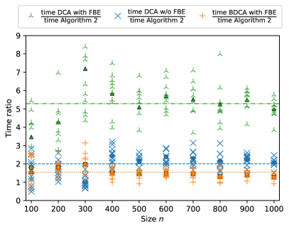
As DCA with FBE was clearly the slowest method, we took the function value of the solution returned by DCA without FBE as the target value for both Algorithm 2 and BDCA, so these algorithms were stopped when that function value was reached. In Figure 8, we plot the time ratio of each algorithm against Algorithm 2. On average, Algorithm 2 was more than 5 times faster than DCA with FBE and more than 2 times faster than DCA without FBE. BDCA greatly accelerated the performance of DCA with FBE, but still Algorithm 2 was more than 1.5 times faster. Only for size 300, the performance of DCA without FBE was comparable to that of Algorithm 2. We observe on the right plot that the advantage of Algorithm 2 is maintained for larger sizes.
Experiment 3
With the aim of finding the minimum of a quadratic function with integer and box constraints, we modified the setting of Experiment 2 and considered instead a set composed by balls of various radii centered at , with . As balls of radius cover the region , we ran our tests with balls of radii with . This time we considered both convex and nonconvex objective functions. The nonconvex case was generated as in Experiment 2, while for the convex case, the elements of the diagonal of were chosen as random numbers uniformly distributed in .
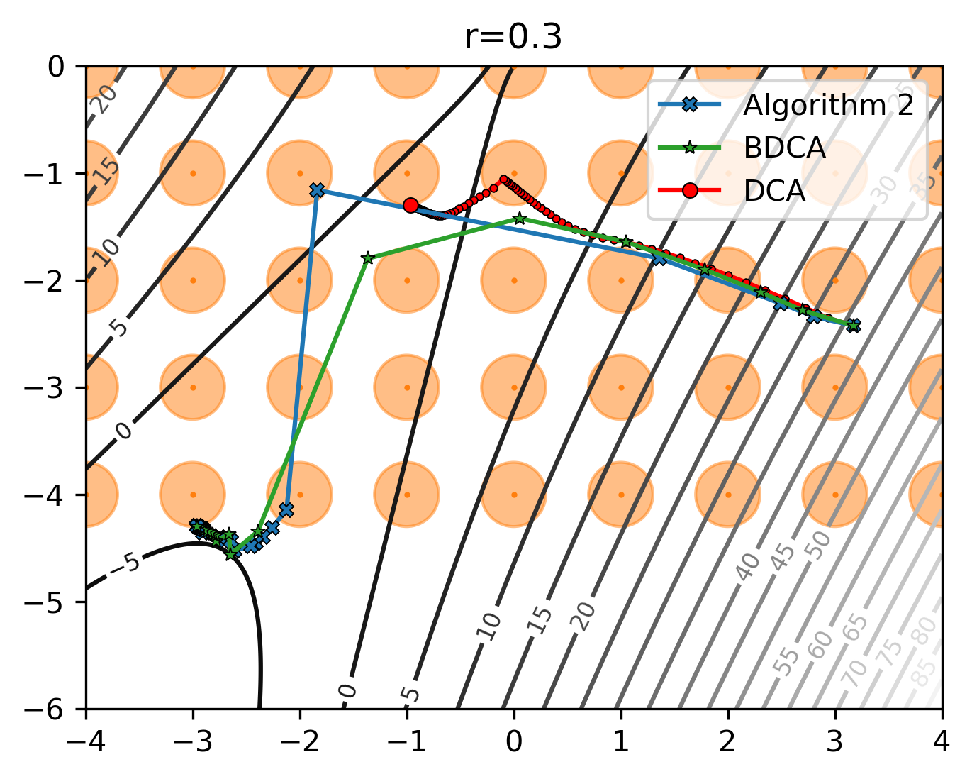
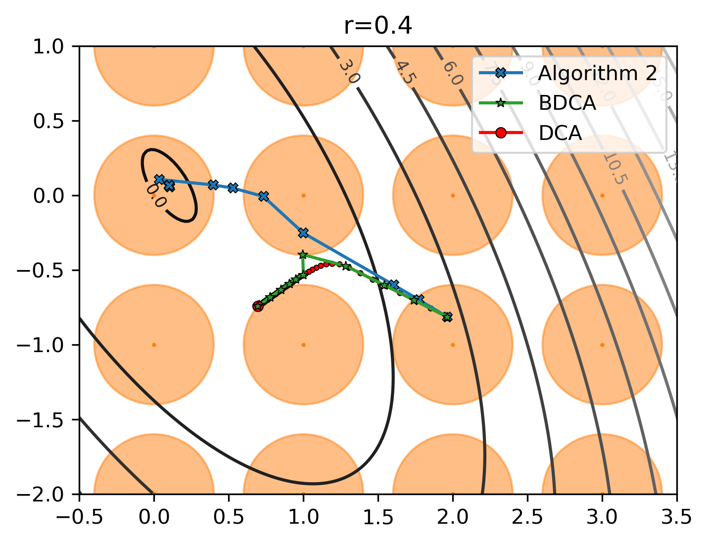
For each and , 100 random instances were generated. For each instance, a starting point was chosen with random coordinates uniformly distributed in . As the constraint sets are nonconvex, FBE was also needed to run DCA. The results are summarized in Table 3, where for each and each radius, we counted the number of instances (out of 100) in which the value of at the rounded output of DCA and BDCA was lower and higher than that of Algorithm 2 when ran from the same starting point. We used the same parameter settings for the algorithms as in Experiment 2. Finally, we plot in Figure 9 two instances in in which Algorithm 2 reached a better solution.
| Radius of the balls | ||||||||||
|---|---|---|---|---|---|---|---|---|---|---|
| 7pt. | Alg. 2 vs | |||||||||
| DCA | 0/34 | 1/20 | 1/26 | 1/19 | 0/19 | 0/18 | 0/3 | 1/1 | 0/2 | |
| BDCA | 6/12 | 2/13 | 3/14 | 4/9 | 0/4 | 1/10 | 0/2 | 1/1 | 0/2 | |
| DCA | 2/89 | 2/83 | 1/66 | 5/53 | 8/28 | 3/7 | 1/1 | 3/1 | 1/0 | |
| BDCA | 21/68 | 38/53 | 33/39 | 23/24 | 18/16 | 2/7 | 0/0 | 0/1 | 0/0 | |
| DCA | 0/99 | 0/98 | 2/87 | 11/58 | 9/32 | 3/8 | 2/9 | 2/2 | 5/4 | |
| BDCA | 16/83 | 29/71 | 40/58 | 37/40 | 13/26 | 2/3 | 0/1 | 0/0 | 1/2 | |
| DCA | 0/100 | 0/100 | 0/91 | 2/86 | 13/41 | 14/12 | 9/12 | 6/10 | 12/12 | |
| BDCA | 8/92 | 6/94 | 31/69 | 36/53 | 16/28 | 8/8 | 6/5 | 3/4 | 5/3 | |
| DCA | 0/100 | 0/100 | 0/99 | 9/87 | 18/49 | 18/31 | 12/22 | 18/20 | 11/21 | |
| BDCA | 2/98 | 6/94 | 39/61 | 36/61 | 23/33 | 16/14 | 9/8 | 9/8 | 13/9 | |
| DCA | 0/100 | 0/100 | 0/100 | 1/98 | 23/64 | 31/41 | 25/29 | 22/30 | 20/41 | |
| BDCA | 3/97 | 2/98 | 38/62 | 37/63 | 33/39 | 27/17 | 18/18 | 14/13 | 16/18 | |
| DCA | 0/100 | 0/100 | 0/100 | 1/99 | 6/94 | 15/80 | 27/61 | 29/65 | 36/48 | |
| BDCA | 0/100 | 1/99 | 41/59 | 44/56 | 33/63 | 25/56 | 34/39 | 32/47 | 17/35 | |
| Radius of the balls | ||||||||||
|---|---|---|---|---|---|---|---|---|---|---|
| 7pt. | Alg. 2 vs | |||||||||
| DCA | 1/8 | 1/9 | 1/10 | 1/6 | 0/6 | 0/6 | 0/8 | 3/2 | 1/0 | |
| BDCA | 2/4 | 1/4 | 1/3 | 3/4 | 0/5 | 0/4 | 0/6 | 3/2 | 1/0 | |
| DCA | 9/39 | 4/39 | 7/39 | 4/35 | 10/30 | 3/27 | 5/45 | 2/34 | 8/29 | |
| BDCA | 9/31 | 11/33 | 13/29 | 6/31 | 11/29 | 6/25 | 7/38 | 5/29 | 10/30 | |
| DCA | 6/69 | 13/67 | 7/62 | 5/61 | 10/53 | 3/59 | 6/56 | 3/72 | 3/66 | |
| BDCA | 16/58 | 16/63 | 16/55 | 12/48 | 9/52 | 11/52 | 13/52 | 12/57 | 11/58 | |
| DCA | 11/81 | 10/79 | 8/87 | 5/90 | 3/87 | 4/80 | 2/86 | 5/89 | 8/81 | |
| BDCA | 24/68 | 21/64 | 23/70 | 17/73 | 14/75 | 9/73 | 10/75 | 18/74 | 16/71 | |
| DCA | 4/96 | 6/94 | 4/94 | 5/94 | 4/96 | 3/97 | 2/98 | 7/91 | 9/91 | |
| BDCA | 15/85 | 16/83 | 18/80 | 14/84 | 17/83 | 11/89 | 9/91 | 20/79 | 19/80 | |
| DCA | 4/96 | 4/96 | 4/96 | 2/98 | 1/99 | 2/98 | 4/96 | 3/97 | 0/100 | |
| BDCA | 11/89 | 16/84 | 11/89 | 8/92 | 6/94 | 11/89 | 10/90 | 13/87 | 8/92 | |
| DCA | 1/99 | 2/98 | 0/100 | 0/100 | 0/100 | 1/99 | 1/99 | 2/98 | 1/99 | |
| BDCA | 12/88 | 17/83 | 15/85 | 9/91 | 15/85 | 11/89 | 9/91 | 18/82 | 20/80 | |
7 Conclusion and Future Research
This paper proposes and develops a novel RCSN method to solve problems of difference programming whose objectives are represented as differences of generally nonconvex functions. We establish well-posedness of the proposed algorithm and its global convergence under appropriate assumptions. The obtained results exhibit advantages of our algorithm over known algorithms for DC programming when both functions in the difference representations are convex. We also develop specifications of the main algorithm in the case of structured problems of constrained optimization and conduct numerical experiments to confirm the efficiency of our algorithms in solving practical models.
In the future research, we plan to relax assumptions on the program data ensuring the linear, superlinear, and quadratic convergence rates for RCSN and also extend the spectrum of applications to particular classes of constrained optimization problems as well as to practical modeling.
References
- (1) Aragón-Artacho, F.J., Goberna, M.A., López, M.A., Rodríguez, M.M.L.: Nonlinear optimization. Springer, Cham (2019)
- (2) Aragón-Artacho, F.J., Geoffroy, M.H.: Metric subregularity of the convex subdifferential in Banach spaces. J. Nonlinear Convex Anal. 15, 35–47 (1014)
- (3) Aragón-Artacho, F.J., Campoy, R., Vuong, P.T.: Using positive spanning sets to achieve d-stationarity with the boosted DC algorithm. Vietnam J. Math. 48, 363–376 (2020)
- (4) Aragón-Artacho, F.J., Campoy, R., Vuong, P.T.: The boosted DC algorithm for linearly constrained DC programming. Set-Valued Var. Anal. 30, 1265–1289 (2022)
- (5) Aragón-Artacho, F.J., Fleming, R.M.T., Vuong, P.T.: Accelerating the DC algorithm for smooth functions. Math. Program. 169, 95–118 (2018)
- (6) Aragón-Artacho, F.J., Vuong, P.T.: The boosted difference of convex functions algorithm for nonsmooth functions. SIAM J. Optim. 30, 980–1006 (2020)
- (7) Asplund, E.: Fréchet differentiability of convex functions. Acta Math. 121, 31–47 (1968).
- (8) Bernard, F., Thibault, L.: Prox-regularity of functions and sets in Banach spaces. Set-Valued Anal. 12, 25–47 (2004)
- (9) Bernard, F., Thibault, L.: Uniform prox-regularity of functions and epigraphs in Hilbert spaces. Nonlinear Anal. 60, 187–207 (2005)
- (10) Colombo, G., Henrion, R., Hoang, N.D.; Mordukhovich, B.S.: Optimal control of sweeping processes over polyhedral control sets. J. Diff. Eqs. 260, 3397–3447 (2016)
- (11) de Oliveira, W.: The ABC of DC programming. Set-Valued Var. Anal. 28, 679–706 (2020)
- (12) Ding, C., Sun, D., Ye, J.J.: First-order optimality conditions for mathematical programs with semidefinite cone complementarity constraints. Math. Program. 147, 539–379 (2014)
- (13) Drusvyatskiy, D., Mordukhovich, B.S., Nghia, T.T.A.: Second-order growth, tilt stability, and metric regularity of the subdifferential. J. Convex Anal. 21, 1165–1192 (2014)
- (14) Facchinei, F., Pang, J.-S.: Finite-Dimensional Variational Inequalities and Complementarity Problems, I, II. Springer, New York (2003)
- (15) Gfrerer, H., Outrata, J.V.: On a semismooth∗ Newton method for solving generalized equations. SIAM J. Optim. 31, 489–517 (2021)
- (16) Henrion, R., Mordukhovich, B.S., Nam, N.M.: Second-order analysis of polyhedral systems in finite and infinite dimensions with applications to robust stability of variational inequalities. SIAM J. Optim. 20, 2199–2227 (2010)
- (17) Henrion, R., Outrata, J., Surowiec, T.: On the co-derivative of normal cone mappings to inequality systems. Nonlinear Anal. 71, 1213–1226 (2009)
- (18) Henrion, R., Römisch, W.: On -stationary points for a stochastic equilibrium problem under equilibrium constraints in electricity spot market modeling. Appl. Math. 52, 473–494 (2007)
- (19) Hiriart-Urruty, J.-B.: Generalized differentiability, duality and optimization for problems dealing with differences of convex functions. In: Ponstein, J. (ed.) Convexity and Duality in Optimization. Lecture Notes Econ. Math. Syst. 256, pp. 37–70. Springer, Berlin (1985)
- (20) Izmailov, A.F., Solodov, M.V.: Newton-Type Methods for Optimization and Variational Problems. Springer, Cham (2014)
- (21) Khanh, P.D., Mordukhovich, B.S., Phat, V.T.: A generalized Newton method for subgradient systems. Math. Oper. Res. (2022), DOI 10.1287/moor.2022.1320
- (22) Khanh, P.D., Mordukhovich, B.S., Phat, V.T., Tran, D.B.: Generalized Newton algorithms in nonsmooth optimization via second-order subdifferentials. J. Global Optim. (2022). DOI 10.1007/s10898-022-01248-7
- (23) Khanh, P.D., Mordukhovich, B.S., Phat, V.T., Tran, D.B.: Globally convergent coderivative-based generalized Newton methods in nonsmooth optimization (2022). arXiv:2109.02093
- (24) Li, W., Bian, W., Toh, K.-C.: Difference-of-convex algorithms for a class of sparse group regularized optimization problems. SIAM J. Optim. 32, 1614–1641 (2022)
- (25) Mordukhovich, B.S.: Sensitivity analysis in nonsmooth optimization. In: Field, D.A., Komkov, V.(eds) Theoretical Aspects of Industrial Design, pp. 32–46. SIAM Proc. Appl. Math. 58. Philadelphia, PA (1992)
- (26) Mordukhovich, B.S.: Variational Analysis and Generalized Differentiation, I: Basic Theory, II: Applications. Springer, Berlin (2006)
- (27) Mordukhovich, B.S.: Variational Analysis and Applications. Springer, Cham (2018)
- (28) Mordukhovich, B.S., Outrata, J.V.: On second-order subdifferentials and their applications. SIAM J. Optim. 12, 139–169 (2001)
- (29) Mordukhovich, B.S., Rockafellar, R.T.: Second-order subdifferential calculus with applications to tilt stability in optimization. SIAM J. Optim. 22, 953–986 (2012)
- (30) Mordukhovich, B.S., Sarabi, M.E.: Generalized Newton algorithms for tilt-stable minimizers in nonsmooth optimization. SIAM J. Optim. 31, 1184–1214 (2021)
- (31) Moré, J.J., Sorensen, D.C.: Computing a trust region step. SIAM J. Sci. Statist. Comput. 4. 553–572 (1983)
- (32) Ostrowski, A.M.: Solution of Equations and Systems of Equations, 2nd ed. Academic Press, Cambridge, MA (1966)
- (33) Outrata, J.V., Sun, D.: On the coderivative of the projection operator onto the second-order cone. Set-Valued Anal. 16 (999-1014 (2008)
- (34) Patrinos, P., Bemporad, A.: Proximal Newton methods for convex composite optimization. In: 52nd IEEE Conf. Dec. Cont., pp. 2358–2363. Florence, Italy (2013)
- (35) Rockafellar, R.T., Wets, R.J-B.: Variational Analysis. Springer, Berlin (1998)
- (36) Tao, P.D., An, L.T.H.: Convex analysis approach to DC programming: theory, algorithms and applications. Acta Math. Vietnam. 22, 289–355 (1997)
- (37) Tao, P.D., An, L.T.H.: A DC optimization algorithm for solving the trust-region subproblem. SIAM J. Optim. 8, 476–505 (1998)
- (38) Tao, P.D., Bernoussi, E.S.: Algorithms for solving a class of nonconvex optimization problems. Methods of subgradients. North-Holland Math. Stud. 129, 249–271 (1986)
- (39) Themelis A., Stella, L. and Patrinos, P.: Forward-backward envelope for the sum of two nonconvex functions: further properties and nonmonotone linesearch algorithms. SIAM J. Optim. 28, 2274–2303 (2018)
- (40) Toland, J.F.: On subdifferential calculus and duality in non-convex optimization. Mem. Soc. Math. France. 60, 177–183 (1979)
- (41) Truong, T.T., Nguyen, H.T.: Backtracking gradient descent method and some applications in large scale optimisation, II: Algorithms and experiments. Appl. Math. Optim. 84, 2557–2586 (2021)
- (42) Yao, J.-C., Yen, N.D.: Coderivative calculation related to a parametric affine variational inequality. Part 1: Basic calculation. Acta Math. Vietnam. 34, 157–172 (2009)