Bridging High-Density, Electron Beam Coronal Transport and Deep Chromospheric Heating in Stellar Flares

Abstract

The optical and near-ultraviolet (NUV) continuum radiation in M dwarf flares is thought to be the impulsive response of the lower stellar atmosphere to magnetic energy release and electron acceleration at coronal altitudes. This radiation is sometimes interpreted as evidence of a thermal photospheric spectrum with $T\approx 10^{4}$ K. However, calculations show that standard solar flare coronal electron beams lose their energy in a thick target of gas in the upper and middle chromosphere (log₁₀ column mass /[g cm^-2] $\lesssim-3$). At larger beam injection fluxes, electric fields and instabilities are expected to further inhibit propagation to low altitudes. We show that recent numerical solutions of the time-dependent equations governing the power-law electrons and background coronal plasma (Langmuir and ion-acoustic) waves from Kontar et al. produce order-of-magnitude larger heating rates than occur in the deep chromosphere through standard solar flare electron beam power-law distributions. We demonstrate that the redistribution of beam energy above $E\gtrsim 100$ keV in this theory results in a local heating maximum that is similar to a radiative-hydrodynamic model with a large, low-energy cutoff and a hard power-law index. We use this semi-empirical forward modeling approach to produce opaque NUV and optical continua at gas temperatures $T\gtrsim 12,000$ K over the deep chromosphere with log₁₀ column mass /[g cm^-2] of $-1.2$ to $-2.3$. These models explain the color temperatures and Balmer jump strengths in high-cadence M dwarf flare observations, and they clarify the relation among atmospheric, radiation, and optical color temperatures in stellar flares.

1 Introduction

Empirical, multi-wavelength relationships in solar and stellar flares are consistent with similar physical processes of magnetic reconnection, particle acceleration, and atmospheric heating (Hawley et al., 1995; Guedel et al., 1996; Neupert, 1968; Dennis & Zarro, 1993). However, non-negligible optical depths from plasma at $T\approx 10,000$ K in the near-ultraviolet (NUV) and optical continuum are critical in reproducing M-dwarf spectral flare observations (Livshits et al., 1981; Hawley & Fisher, 1992; Kowalski et al., 2015b), which are incompatible with most inferences from solar flare observations in the optical (Potts et al., 2010) and NUV (Heinzel & Kleint, 2014; Kleint et al., 2016; Kowalski et al., 2017a; Dominique et al., 2018). Lower rates of atmospheric excitation result in smaller electron densities and optical depths in solar flare chromospheres (Neidig, 1983; Kowalski et al., 2022). In solar flare chromospheric heating models, the only self-consistent predictions of optically thick flare continua originate from relatively small temperature increases, $\Delta T\approx 500-1000$ K in the radiatively backwarmed photosphere (Neidig et al., 1993; Allred et al., 2005, 2006; Cheng et al., 2010; Kowalski et al., 2017a, see also Kleint et al. 2016). However, it is unclear whether solar spectra have yet sampled the brightest sources and whether there is more optically thick continuum radiation at certain very bright sources than models predict in solar flares. There is a variety of spectra in the optical and $U$ band that have been reported in solar flares (Neidig, 1983; Neidig et al., 1993; Kowalski et al., 2015a; Procházka et al., 2017), which is evidence that the comprehensive processes that heat the chromosphere and photosphere are not fully understood.

Large continuum optical depths in M dwarf flares have been achieved through static, semi-empirical modeling (Cram & Woods, 1982; Christian et al., 2003; Fuhrmeister et al., 2010; Kowalski et al., 2011) and in radiative-hydrodynamic (RHD) modeling with extremely large electron beam flux densities of $10^{13}$ erg cm^-2 s^-1 distributed with a power-law index, $\delta\approx 3-4$, above a low-energy cutoff of $E_{c}\approx 30-40$ keV (Kowalski et al., 2015b). These particular electron beam parameters were inferred from collisional thick target modeling of hard X-ray and gamma ray spectra of the large 2002 July 23 X4.5 solar flare (Holman et al., 2003; White et al., 2003; Allred et al., 2006; Ireland et al., 2013). The collisional thick target model (Brown, 1971) assumes that Coulomb collisions dominate the energy loss (e.g., Emslie, 1978; Leach & Petrosian, 1981) of nonthermal electrons as they radiate hard X-rays in the thick target chromosphere (see Brown et al. 2009 and Kontar et al. 2011 for overviews). It is the most widely used framework (e.g., Milligan et al., 2014; Kleint et al., 2016; Dennis & Tolbert, 2019) in forward modeling thermal spectra of solar flare RHD processes (e.g., Allred et al., 2005; Rubio da Costa et al., 2016; Kowalski et al., 2017a; Sadykov et al., 2019; Graham et al., 2020) and in hypothesis testing of X-ray spectra of stellar superflares (Osten et al., 2007, 2016). In recent higher spatial resolution solar observations of chromospheric/photospheric flare footpoint sources, Krucker et al. (2011) infer high electron beam fluxes of $10^{12}-10^{13}$ erg cm^-2 s^-1 above $18-20$ keV under the assumptions of the standard collisional thick target model. They interpret this beam flux range to mean that there is a severe, systematic flaw (e.g., Smith, 1975; Brown & Melrose, 1977) in the standard assumptions. Magnetic field convergence (Kontar et al., 2008) has been briefly mentioned as a potential solution (Brown et al., 2009), but Krucker et al. (2011) exclude this explanation in their analysis. In a limb flare, Martínez Oliveros et al. (2012) directly imaged white-light and hard X-ray source heights and found lower altitudes than expected through state-of-the-art modeling of time-independent electron beam transport from a coronal source (e.g., Battaglia et al., 2012).

Some radio observations of gyrosynchrotron emission also point to very large nonthermal electron densities of $n_{e}\approx 10^{10}$ cm^-3 in the corona (White et al., 2003; Raulin et al., 2004; Kundu et al., 2009; White et al., 2011; Kawate et al., 2012); these measurements are not dependent on the assumptions of the collisional thick target model for hard X-rays. In the 2002 July 23 solar flare, White et al. (2003) discuss that the similarity between the radio light curves from the dense, $n_{e}\approx 10^{10}$ cm^-3, coronal flare sources and from the hard X-ray footpoint sources implies origins from the same population of accelerated electrons. Most recently, unprecedented observations from the Expanded Owens Valley Solar Array have shown that ambient particles evacuate into a nonthermal distribution over large coronal volumes (Fleishman et al., 2022). These persistent sources are attributed to a trapping mechanism that is yet to be specified.

If the dense radio-emitting sources precipitate as large fluxes into the chromosphere at the locations of the bright solar flare kernels, non-collisional transport physics must be considered. The relative displacement of the accelerated electrons and protons generates a strong electric field that drives a cospatial return current (drifting Maxwellian) of the ambient electrons. The neutralizing return current is also required to prevent enormous magnetic fields. A large beam current density decelerates in this electric field and loses its energy to the background plasma through Joule heating (Holman, 2012). Some analytic calculations suggest this may occur over just several hundred meters (van den Oord, 1990).

It is generally thought that large beam densities cannot even form before steady state, or the beams should mostly confine themselves to the coronal acceleration region in the presence of electric field double layers that rapidly develop in response to large relative drift velocities between the ambient electrons and ions (e.g., Li et al., 2012, 2014). Lee et al. (2008) simulate a very hot Maxwellian beam and calculate the energy loss due to plasma instabilities. They suggest that the highest-energy electrons in the beam propagate to the footpoints with less energy loss than the lower energy particles, which thermalize. For a power-law distribution, however, there are relatively few electrons in the high-energy tail to begin with. Other calculations predict very large amounts of energy loss, $\approx 0.6m_{i}c_{\rm{Alfven}}^{2}$, during beam passage through a series of double-layer electric fields (Li et al., 2014). Thus, hard X-ray footpoint sources would be dominated by thermal emission if the bulk of beam energy thermalizes during coronal transport, which is contrary to their well-understood properties that include nonthermal electron bremsstrahlung radiation at $E\approx 25-300$ keV, gamma-ray nuclear excitation lines, and electron-positron annihilation radiation (Vilmer et al., 2011; Dennis et al., 2022). Moreover, beam energy loss in the corona and subsequent thermal conduction into the chromosphere produce faint continuum radiation (Kowalski et al., 2017a) and are not able to explain large optical depths and hydrogen line broadening in M dwarf flare observations (Namekata et al., 2020). On the other hand, updated hydrogen pressure broadening in the RHD models of Kowalski et al. (2015b) and Kowalski et al. (2016) suggest that the “scaled-up” beam fluxes that are characterized by power-law parameters, as inferred from solar flare hard X-rays, produce chromospheric condensations that are far too dense to be consistent with optical stellar spectra (Kowalski et al., 2017b; Kowalski, 2022).

An alternative heating mechanism to extreme-flux, electron-beam distributions that are inferred from standard collisional thick target modeling of solar flares is warranted to explain the deep chromospheric heating in M dwarf flares while also accounting for transport effects due to large coronal beam densities. This topic is timely in the context of the many thousands of white-light stellar flares that have recently been reported in data from Kepler, K2, and TESS (e.g., Hawley et al., 2014; Maehara et al., 2021). The potential impact of ultraviolet flares is also developing into an important issue facing assessments of exoplanet habitability (e.g., Loyd et al., 2018; Howard et al., 2018; Tilley et al., 2019; Howard et al., 2020; Abrevaya et al., 2020). One such alternative modeling approach is explored in Kowalski et al. (2017b), where they extend the standard electron beam modeling paradigm to larger, low-energy cutoff values ($E_{c}=85-500$ keV) than typically inferred ($E_{c}\approx 15-25$ keV) in solar flares, aside from a few instances reported in late impulsive peaks (Holman et al., 2003; Warmuth et al., 2009). In Kowalski (2022), we develop this modeling approach further for comparisons to the entire observed hydrogen Balmer line series in stellar flare spectra from Hawley & Pettersen (1991), and we achieve statistical agreement with the rise and peak phase. However, physical justification for large, low-energy cutoffs of accelerated electron distributions in M dwarf flares has not been formulated. Here, we report on extensions to the modifications of the collisional thick target model that are developed in Kontar et al. (2012); hereafter K12. We show that the time-dependent, coronal transport calculations of K12 produce beam heating distributions in the pre-flare, low chromosphere that are remarkably similar to electron beams with large, low-energy cutoffs ($E_{c}\approx 85$ keV) and hard ($\delta\approx 3$) power-law indices.

The paper is organized as follows. In Section 2.1, we describe the RHD flare model setup. We analyze several RHD flare models with large, low-energy cutoffs that generate optical depths in the NUV and optical continuum in the low chromosphere (Section 2.2). We compare the highest-flux model to high-cadence optical flare colors that were reported recently in the literature (Section 2.2.1). In Section 2.3, we present new calculations of the initial chromospheric heating profiles using the time-averaged electron beam spectra in K12, and we compare them to the models that provide new interpretations of the flare data. In Section 3, we discuss the implications for future modeling efforts of solar and stellar flares. In Section 4, the main conclusions of this work are presented.

2 RHD Flare Modeling with RADYN

Before presenting heating rates from the modified beam distribution of K12, we establish that deep atmospheric heating from a large, low-energy cutoff electron beam model and an extremely high energy flux produce large continuum optical depths at $\lambda=3615$ Å, $4170$ Å, and $6010$ Å. We analyze the formation of the continuum radiation at these wavelengths, and we explain how hot, optical color temperatures ($T_{\rm{col}}\approx 10^{4}$ K) in spectral observations originate in these models. To establish the importance of the K12 theory for this phenomenological characteristic of stellar flares, we compare to constraints from high-cadence flare colors during the rise and peak phases throughout a giant dMe flare event that was reported in Kowalski et al. (2016).

2.1 Electron Beam Heating with Large Low-energy Cutoffs: Model Setup

We have calculated a comprehensive grid of RHD models with the RADYN code (Carlsson & Stein, 1992, 1995, 1997, 2002; Allred et al., 2015). The details about the setup will be described in a separate paper (Kowalski et al. 2023, in preparation), but a brief summary is presented here. The effective temperature of the starting atmosphere is $T_{\rm{eff}}\approx 3600$ K (see the Appendix of Kowalski et al., 2017b, for details regarding the starting atmosphere). The equations of mass, momentum, internal energy, and charge are solved on an adaptive grid (Dorfi & Drury, 1987) with the equations of radiative transfer and level populations for hydrogen, helium, and Ca II. To simulate flare heating, we model the energy deposition from a power-law distribution of electrons, which is calculated in a 1D magnetic loop of half-length $10^{9}$ cm, a constant surface gravity of log $g=4.75$, and a uniform cross-sectional area. The electron beam is injected at the loop apex, which has an ambient electron density ($n_{e}$) of $3\times 10^{10}$ cm^-3 and a gas temperature ($T_{\rm{gas}}$) of 5 MK. The atmospheric response is calculated with a ramping beam flux to a maximum value at $t=1$ s, followed by a decrease until $t=10$ s according to the pulsed injection profile prescription in Aschwanden (2004). We assume that the injected pitch angle distribution is Gaussian-distributed in $\mu=\cos\theta$ (where $\mu=1$ is directed along the magnetic loop axis) in the forward hemisphere with a spread of $\sigma_{\mu}=0.07$. The heating rates as a function of atmospheric depth at each time step in the RHD simulations are calculated from the steady-state solution of the Fokker-Planck equation for Coulomb energy loss to neutrals and charged particle constituents; this solver was recently developed into the FP code (Allred et al., 2020). In this first-generation M dwarf flare model grid, return current and magnetic mirroring forces are not included as external force terms. Thus, these RHD simulations capture the physics of “free-streaming” electron beam propagation. In general terms, these models are consistent with the assumptions of the collisional thick target model of hard X-rays. The peak injected beam energy fluxes span four orders of magnitude: $10^{10}$ (F10), $10^{11}$ (F11), $10^{12}$ (F12), and $10^{13}$ (F13) erg cm^-2 s^-1. The low-energy cutoffs in the grid range from $E_{c}=17$ keV to 500 keV. The selected pulsed injection models for this study have $E_{c}=85$ keV and injected electron beam number fluxes with a power-law index of $\delta=3$, which is consistent with available stellar flare constraints (Osten et al., 2007; MacGregor et al., 2018, 2020, 2021). We refer to these models as mF10-85-3, mF11-85-3, mF12-85-3, and mF13-85-3. Following Kowalski et al. (2017a) and the appendices of Kowalski et al. (2017b), the contribution functions ($C_{I}$) to the emergent intensity, the optical depths ($\tau$), and the radiation (brightness) temperatures ($T_{\rm{rad}}$) at several continuum wavelengths are analyzed at a viewing angle corresponding to $\mu^{\prime}=\cos\theta^{\prime}=0.95$ at a time of $t=1$ s. This time corresponds to the maximum beam energy injection into the atmosphere. A corresponding grid of models is calculated using a constant (“c”) beam flux injection; the initial heating rate at $t=0$ s for the constant injection model, cF13-85-3, is discussed in Section 2.3. The optical depth calculations in Section 2.2 are nearly identical for the constant flux injection models at $t=1$ s; therefore, we choose to analyze in detail the ramping beam injection calculations that modeled low-time resolution spectral data of a dMe flare in Kowalski (2022).

2.2 Model Continuum Spectrum Analysis

The range of maximum beam fluxes from the mF10-85-3 model to the mF13-85-3 model establishes a threshold at which non-negligible continuum optical depths develop over the low atmosphere as a function of wavelength. Figure 1(a) shows the gas temperature response of the M dwarf atmosphere at $t=1$ s in each model. The vertical dashed lines indicate the locations of $\tau=0.95$ at the continuum wavelength of $\lambda=3615$ Å, which is a representative wavelength on the blue side of the Balmer jump. As the maximum beam flux of the model increases to the F13 level, the effective photosphere at this wavelength shifts up to the column mass (log${}_{10}\ m$ / [g cm^-2]) range between $\approx-1.7$ and $-2.0$, which corresponds to the lower chromosphere in the preflare state. In the mF13-85-3, the $\tau\approx 1$ layer occurs at $T_{\rm{gas}}\approx 13,500$ K. The NUV flare photosphere occurs at a cooler temperature, $T_{\rm{gas}}\approx 9000$ K, in the mF12-85-3 simulation, but the optical depth variation at $\lambda=3615$ Å as a function of column mass (not shown) is rather similar to the mF13-85-3.

Figure 1: (a) The atmospheric gas temperature response to electron beam-heating models with $E_{c}=85$ keV at $t=1$ s after injection into a model M dwarf atmosphere. The vertical dashed lines indicate the column masses at which $\tau=0.95$ occur in the continuum wavelength at $\lambda=3615$ Å. The preflare gas temperature ($t=0$ s) is shown for comparison. (b) The variation of the optical depth at $\lambda=4170$ Å exhibits marked differences between the mF12-85-3 and mF13-85-3 models at $t=1$ s in their respective evolution. The gas temperature of the mF13-85-3 model is reproduced from panel (a). The contribution function ($C_{I}$) to the emergent intensity at three continuum wavelengths in the mF13-85-3 model at $t=1$ s is displayed in units of erg cm^-2 s^-1 Å^-1 s.r.^-1 (unit log₁₀ col mass)^-1 on a linear scale with arbitrary peak normalization.

In Figure 1(b), the mF13-85-3 and mF12-85-3 models clearly differ in the optical depths at longer continuum wavelengths. The variation of $\tau$ at $\lambda=4170$ Å  (shown for the mF13-85-3 and mF12-85-3 models) confirms that only the mF13-85-3 model produces significant optical depth in the significantly heated regions of the deep chromosphere around log${}_{10}\ m\approx-1.5$, which becomes the optical flare photosphere at $t=1$ s. The contribution functions to the emergent intensity at $\lambda=4170$ Å, $\lambda=6010$ Å, and $\lambda=3615$ Å are shown from the mF13-85-3 model in Figure 1(b). The continuum at $\lambda=4170$ Å is formed over a deeper range of column mass at $t=1$ s than the NUV continuum intensity at $\lambda=3615$ Å and the red-optical continuum intensity at $\lambda=6010$ Å. Among all NUV, optical, and near-infrared continuum wavelengths, the blue-optical wavelengths at $\lambda\approx 4000-4200$ Å are the most optically thin at $T_{\rm{gas}}\approx 10^{4}$ K. Note that of the semi-empirical, static models in Cram & Woods (1982), their model # 5 is most similar to the mF13-85-3 atmospheric state at $t=1$ s. In the appendices of Kowalski et al. (2017b), similar contribution functions at $\lambda=4170$ Å  for two models with lower beam fluxes and larger, low-energy cutoffs are described. In the next section, we connect the multi-wavelength continuum formation from the mF13-85-3 model to the broadband continuum shape in the impulsive phase of a large M dwarf flare.

2.2.1 Comparison to High-cadence Flare Color Observations

The emergent radiative flux and intensity predictions from the mF13-85-3 model are consistent with spectral observations of the impulsive phase of some M dwarf flares. Specifically, the measured spectral quantities that motivate large heating rates are small Balmer jump ratios and hot, NUV, blue-optical, and red-optical color temperatures of $T_{\rm{col}}\approx 10,000-11,000$ K (Mochnacki & Zirin, 1980; Hawley & Pettersen, 1991; Fuhrmeister et al., 2008; Kowalski et al., 2013, 2016, 2018; Kowalski, 2022). Two sequential, high-energy flare events that occurred on the M-dwarf YZ CMi are shown in Figure 2. These events were observed in three narrowband continuum filters with central wavelengths at $\lambda_{\rm{cen}}=3500$ Å, $4170$ Å, and $6010$ Å using the ULTRACAM instrument (Dhillon et al., 2007). These flares were studied in detail in Kowalski et al. (2016), and are referred to as the “IF1” and “IF3” events in that work. Following the method of Hawley et al. (1995), we solve for blackbody color temperatures through Newton-Raphson linearization and iteration constrained to the $\lambda_{\rm{cen}}=4170$ Å and $\lambda_{\rm{cen}}=6010$ Å continuum-filter ratios that are reported in Kowalski et al. (2016).

Broadband, white-light color temperatures of $T_{\rm{col}}=9,000-11,000$ are attained over the rise, peak, and initial fast-decay phases of these events. The flares in Figure 2 exhibit the highest-time resolution constraints on the broadband color temperature evolution in a dMe flare event. Similar hot, blue-optical color temperatures were calculated from spectra during the rise, peak, and fast decay phase during another large-amplitude event on YZ CMi in Kowalski et al. (2013), and a detailed comparison of hot color temperatures from simultaneous spectra and ULTRACAM photometry were analyzed in smaller-amplitude events after IF3 in Kowalski et al. (2016). The evolution of the color temperature to cooler values after each major peak in Figure 2 has been reported in spectra of the gradual decay phases of other large dMe flares (see Fig. 31 of Kowalski et al., 2013), which indicate that a single-continuum model is unable to explain the full optical continuum distribution. Here, we focus on the hotter phases of the IF1 and IF3 events, which have long-challenged models with lower flux electron beams and X-ray backwarming (e.g., Hawley & Fisher, 1992; Allred et al., 2006). The phenomenological “9000 K blackbody hypothesis” is widely adopted to facilitate calculating flare energies and ultraviolet fluxes using extrapolations from single-bandpass Kepler, K2, and TESS optical/infrared photometry (e.g., Shibayama et al., 2013; Günther et al., 2020; Chen et al., 2021). A self-consistent physical explanation, as follows, of the relatively short but luminous phases around each major peak in Figure 2 is of broad significant astrophysical interest.

Thus, we further analyze the emergent continuum intensity, radiation temperature, and contribution function dependencies on wavelength from the mF13-85-3 model at $t=1$ s in order to explain the hottest values of $T_{\rm{col}}\approx 10,000-11,000$ K in the ULTRACAM data of the YZ CMi flare events in Figure 2. The continuum intensity at $\lambda=4170$ Å is more optically thin and thus forms over slightly deeper, cooler temperatures (Figure 1b) than at $\lambda=6010$ Å. Consequently, the radiation temperatures of the model spectra at $\lambda=4170$ Å and $\lambda=6010$ Å are $T_{\rm{rad}}=13,200$ K and $14,100$ K, respectively. From the respective emergent continuum intensity ratios, we solve for a color temperature of $T_{\rm{col}}=10,900$ K, which is consistent with the color temperatures from the ULTRACAM filter ratios (Figure 2). However, the model $T_{\rm{col}}$ is below the atmospheric gas temperature range, $T_{\rm{gas}}\approx 12,000-20,000$ K, over which 90% of the emergent optical and NUV continuum intensity originates. This hot and heterogeneously stratified atmospheric temperature structure is fully consistent with a color temperature in the emergent spectrum that is apparently cooler and isothermal, $T_{\rm{col}}\approx 9000-11,000$ K. We find the following approximate relationship among these temperature measures: $T_{\rm{rad}}\approx T_{\rm{gas}}(\tau\approx 0.3)>T_{\rm{col}}$. Thus, color temperatures calculated from spectra are not direct measures of the atmospheric gas temperature in these model atmospheres that exhibit large optical depths in the deep atmosphere. The continuum formation is near local thermodynamic equilibrium (LTE), but the Eddington-Barbier relation is not an accurate simplification of the continuum formation because $T_{\rm{rad}}\neq T_{\rm{gas}}(\tau=0.95)$. Similar analyses explain the small model Balmer jump ratio, which is consistent with the measured ratios of the $\lambda\approx 3500$ Å to $\lambda\approx 4170$ Å fluxes (see Kowalski et al., 2016) over the times shown in Figure 2.

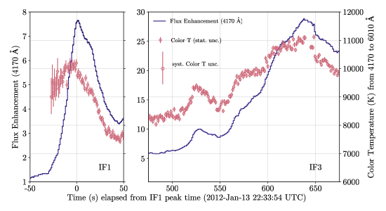
Figure 2: High-cadence ($\Delta t=1.1$ s) ULTRACAM photometry in the NBF4170 ($\lambda_{\rm{cen}}=4170$ Å) narrowband continuum filter during two sequential flare events (IF1 and IF3) on the dM4.5e star YZ CMi. The photometry is normalized to 1.0 during quiescence, and the statistical photometry errors are plotted but are small on this scale. The flux-calibrated, quiescent-subtracted NBF4170 and the RC#1 ($\lambda_{\rm{cen}}=6010$ Å) data are converted to filter ratios. We solve for the optical color temperatures ($T_{\rm{col}}$), which are referred to as FcolorR in the study of these events in Kowalski et al. 2016. Representative systematic uncertainties on the color temperatures are indicated as ${}^{+600}_{-550}$ K and are obtained from the uncertainties in the absolute flux calibration. Note that detailed comparisons of spectra to ULTRACAM filter ratios in smaller-amplitude flares that occurred later in these observations have revealed that values of TFcolorR $\approx 10,000$ K are systematically smaller by $\approx 2000$ K compared to the color temperatures that are fit to the blue-optical spectral range at $\lambda=4000-4800$ Å  (see Kowalski et al., 2016, for details about the data, flare colors, and error analysis).

2.3 Electron-beam Generated Langmuir and Ion-acoustic Turbulence

Electron beams with high-energy fluxes ($\gtrsim 10^{12}$ erg cm^-2 s^-1) and large low-energy cutoffs ($E_{c}\gtrsim 80$ keV) are therefore well-justified, semi-empirical models for the heating rates that generate continuum optical depths in the low atmosphere during M-dwarf flares (see also Kowalski, 2022) at very high-time resolution. There are many implications for models of the Balmer jump, NUV, and Balmer line broadening that are outside the scope of this paper but will be presented in future work. These applications include models of less impulsive flare types that exhibit larger Balmer jumps and smaller optical color temperatures (Kowalski et al., 2019b), flares that exhibit Balmer jumps in absorption and hotter optical color temperatures (Kowalski et al., 2017b) than the events in Figure 2, and the evolution of the flare colors through the gradual decay phase (e.g., in Figure 2). We now turn to the main result of this work in which we propose the physical origin for stellar flare electron beams with effective low-energy cutoffs of $E_{c}\gtrsim 85$ keV and hard power-law indices. This result draws on and connects to theoretical foundations that have been recently developed to modify the collisional thick target model of solar flare hard X-ray emission.

The propagation of electron beams on very short timescales, $\Delta t\ll 1$ s, after the initial acceleration process(es) has been investigated with collisionless (Vlasov-Maxwell), particle-in-cell (PIC) simulations (see Arber et al., 2015; Nishikawa et al., 2021, for modern reviews and discussions of recent progress). Alternatively, numerical solutions over longer timescales are possible for the set of coupled equations consisting of a collisional, time-dependent equation that governs the electron (beam$+$plasma) phase-space evolution and an equation that governs the evolution of background plasma wave energy (K12; see also Hamilton & Petrosian 1987; Kontar 2001; Kontar & Pécseli 2002; Hannah et al. 2009, 2013; Ratcliffe & Kontar 2014; Thorne & Blandford 2017). The component of the distribution function for the background plasma represents the evolution of longitudinal plasma waves, which consist of ambient electron disturbances (Langmuir waves) and ion sound waves (ion-acoustic waves). K12 solve these equations over $\Delta t=1$ s of electron beam propagation through the solar corona with random (Gaussian) density perturbations simultaneously with non-linear, three-wave interactions (e.g., Tsytovich, 1995, and Ch. 23.3.6 of Thorne & Blandford 2017) and a term for collisional energy loss from the beam particles. To briefly summarize the results that are relevant to this work, the kinetic energy losses of low-energy beam electrons generate Langmuir waves, which evolve in angular wavenumber ($k$) space through wave-wave processes (and through refraction and diffusion). The wave turbulence transfers energy back to the beam, resulting in effective energy gains of $dE/dt\gtrsim 200$ keV s^-1 per beam electron at $E\approx 100-400$ keV (see Figs. 4 – 5 of K12).

We demonstrate that the enhancements of the numbers of beam electrons with $E\gtrsim 100$ keV at the expense of the numbers at $E\lesssim 60$ keV as a result of the energy transfer mechanisms in K12 effectively produce an energy deposition peak in the low chromosphere that is similar to the large, low-energy cutoff beams in Section 2. The time-averaged electron beam flux spectra (reproduced in Figure 3(a) here) from Fig. 4 of K12 are injected into a model M dwarf atmosphere from Section 2 to quantify the beam heating in a realistic model stellar chromosphere. Hereafter, we refer to the beam flux spectrum from K12 that includes three-wave non-linear processes as the “wave$+$wave, beam$+$wave” simulation. We solve the steady-state energy deposition with the Fokker-Planck module from McTiernan & Petrosian (1990) that was incorporated into RADYN for the flare simulations in Allred et al. (2015). This version of the RADYN code uniquely includes the capability for an arbitrary particle distribution function to be injected at the loop apex. We assume the same initial Gaussian distribution of pitch angle as for the large $E_{c}$ calculations to facilitate comparison (Section 2.1). The heating profile ($Q_{\rm{beam}}$) for the “wave$+$wave,beam$+$wave” model from K12 is shown for the starting RADYN M dwarf atmosphere in hydrostatic equilibrium in Figure 3(b). Compared to the simulation without “wave$+$wave, beam$+$wave” interactions, the location of the maximum beam heating rate is shifted from the top of the chromosphere to the low chromospheric layers with a large column mass of log${}_{10}\ m\approx-2$. The “wave$+$wave, beam$+$wave” heating rate is an order of magnitude larger at log${}_{10}\ m\approx-2$ than the heating rate without plasma wave-beam interactions. This column mass corresponds to the collisional stopping depths of electrons with initial kinetic energies of $E\approx 100$ keV (Emslie, 1978; Hawley & Fisher, 1994).

In Section 2, we showed the importance of large amounts of heating over the column mass range of log${}_{10}\ m$ from $\approx-1.2$ to $-2.3$ in producing optically thick continuum radiation at NUV and optical wavelengths. We use the cF13-85-3 model calculation at $t=0$ s to show the initial beam heating distribution from a large, low-energy cutoff model in Figure 3(c) for direct comparison to the K12 heating prediction in the undisturbed M dwarf chromosphere. The heating rates are normalized to their respective maximum values of $Q_{\rm{beam}}$. The maximum remarkably corresponds to the same column mass range as the K12 “wave$+$wave, beam$+$wave” calculation. We evaluate the fraction of beam flux lost to the column mass range between log${}_{10}\ m=-2.3$ and $-1.2$ to quantify the similarity. The cF13-85-3 and the K12 models result in fractions of 0.51 to 0.56, whereas standard beam distributions in solar and stellar modeling exhibit much smaller cumulative fractions. A distribution with $E_{c}=40$ keV represents a beam with about the largest cutoff value that is consistent with standard, collisional (cold) thick target modeling of solar flare hard X-rays (e.g. Holman et al., 2003; Ireland et al., 2013); this beam deposits only 0.13 of its energy over the deep chromosphere. More typically, values of $E_{c}=20$ keV or less are inferred; a beam with $\delta=5$ deposits less than 1% of its integrated energy over this column mass range that is important for optically thick continuum formation at $T_{\rm{gas}}\gtrsim 10^{4}$ K.

Figure 3: (a) Nonthermal electron number flux distribution and time-averaged electron number flux distribution with plasma wave interactions, reproduced from Fig. 4 of K12. (b) The initial heating rate from Coulomb collisions in our RADYN M dwarf model chromosphere. (c) The initial Coulomb heating rate in the M dwarf chromosphere for several power-law indices and low-energy cutoffs compared to the K12 heating rate in panel (b). (d) Beam-heating calculations (top panel) for various magnetic field convergence distributions in the chromosphere (bottom panel). The initial gas temperature stratification of the lower M dwarf atmosphere is shown as dashed curves in panels (b)-(d).

3 Discussion

In the absence of mass advection, heating the chromosphere to $T_{\rm{gas}}\gtrsim 10^{4}$ K around log${}_{10}\ m\approx-3$ results in blue continuum radiation that is much more optically thin than heating the chromosphere around log${}_{10}\ m\approx-1.5$ (cf. Figure 1(b)) to a comparable temperature. The column mass range log${}_{10}\ m$ of $-2.3$ to $-1.2$ corresponds to the flare layers that have been previously described as “stationary chromospheric flare layers”, which lie just below the chromospheric condensations in RHD simulations (e.g., Kowalski et al., 2015b). In the large, low-energy cutoff models, upflows develop ($5-20$ km s^-1) due to the thermal pressure gradients over this column mass range, where gas densities deviate from hydrostatic equilibrium at $t\gtrsim 5$ s. The modified electron beam distributions from K12 produce the relative enhancement in the high energy electrons $E\gtrsim 100$ keV that are needed to deliver a significant amount of released magnetic energy to these layers if the total energy flux in the beam is large enough. The models with large low-energy cutoffs ($E_{c}\gtrsim 85$ keV, $\delta\approx 3$) are adequate approximations to the expected RHD response of the K12 beam in deep regions of the atmosphere.

In future work, it will be important to also consider the upper atmospheric evolution in response to the injection of K12 electron beams. Based on results from previous RHD models, we can make several qualitative predictions. We expect the low-energy electrons to readily increase the temperature of the corona and transition region through direct collisional heating and through the steady-state return current heating (Allred et al., 2020), which has not yet been included in M dwarf flare models. We expect these energy loss mechanisms to drive chromospheric condensations (e.g., Graham et al., 2020), which may build up continuum optical depths as they cool to $T_{\rm{gas}}\approx 10^{4}$ K. Even without return current force terms, the larger Coulomb heating rates in the upper chromosphere of the K12 prediction in Figure 3(c) would likely generate chromospheric condensations that are not present in the beams with the larger low-energy cutoffs ($E_{c}\geq 85$ keV, $\delta=3$). Furthermore, rapid thermal ionization of the chromosphere causes the beam heating to shift higher up within the chromosphere, and evaporation of chromospheric material eventually stops the low-energy particles in the low flare corona. Magnetic field convergence in the low atmosphere is an additional external force that may shift the beam heating farther up in the chromosphere.

To evaluate the degree to which magnetic field convergence affects large beam fluxes at deep column masses around log${}_{10}\ m\approx-2$, we show several $t=0$ s calculations in Figure 3(d) from the steady-state Fokker-Planck solution with magnetic mirroring of the particles, as described in Allred et al. (2020). We simulate the cF13-85-3 beam, but we widen the initial pitch angle distribution to have a spread of $\sigma_{\mu}=0.18$ in order to accentuate the effects of pitch angle changes due to magnetic mirroring. We follow Battaglia et al. (2012) and model the magnetic field using a hyperbolic tangent:

$$B(z)=2000+1000\tanh\big{(}-\frac{z-z1}{z2}\big{)}$$ (1)

with $z1$ and $z2$ indicated in the figure and $z$ the distance along the loop from $\tau_{500}=1$. Even a carefully placed magnetic wall (convergence model E) does not largely affect the large heating rate maximum in the deep chromosphere. A convergence higher in the chromosphere (model B) still results in a very large heating maximum that is not predicted by standard electron beam distributions inferred through collisional thick target modeling. The upper chromospheric heating more closely approaches the K12 heating rate (Figure 3(b)) in this region, while retaining a large flux into lower altitudes. In convergence models A and B, we expect chromospheric condensations to develop with large heating rates below in the stationary flare layers.

The issue of timescales is possibly a more serious concern in the application of the K12 theory to the heating in a lower flaring atmosphere. The times ($\Delta t=1$ s) over which the K12 flux spectrum (reproduced in Figure 3(a)) is averaged are not consistent with the times of flight, which are on the order of $50-100$ ms, for mildly relativistic electrons to reach the chromosphere. From the calculation in K12, it is not completely evident whether there is enough time for the “wave$+$wave,beam+wave” processes to operate in a wide variety of stellar atmosphere conditions. However, the evolution begins with the onset of the fundamental (bump-on-tail) beam-plasma instability due to collisional loss of the lowest energy electrons, and the timescale for this is faster for larger values of $n_{\rm{beam}}/n_{\rm{background}}$, as expected for high-flux beams in M dwarf coronae; the ambient conditions of M dwarf coronae are briefly discussed below. We also note that the energy transfer processes begin rapidly at $t\ll 1$ s in the calculation of K12 (see the upper right panel of their Fig. 4), but additional calculations with a range of $n_{\rm{beam}}/n_{\rm{background}}$ and temporal averages are probably warranted for input into RHD models of the chromospheric response.

We suggest a modular modeling framework that stitches the current time-dependent K12 and steady-state (e.g. Allred et al., 2020) treatments of transport and heating in future RHD models of M dwarf flares. This is illustrated in a sketch in Figure 4. In panel (a), a reconnected magnetic field line retracts, and a nonthermal electron in the beam bounces back and forth due to a trapping mechanism (e.g., Aschwanden, 2004; Li et al., 2014; Egedal et al., 2015; Fleishman et al., 2022). It is conceivable that trapped beam particles have sufficient time for “wave$+$wave, beam$+$wave” processes to redistribute energy and enhance the number of electrons at $E>100$ keV in this region. The K12 theory is non-magnetic, but our prescription for beam injection into the RADYN model loop (Section 2.1) uses the pulsed injection prescription of Aschwanden (2004) and emulates coronal trapping and injection timescales. The evolution of the loss cone angle in Aschwanden (2004) also might provide a mechanism to preserve beam anisotropy, which is required for the beam-plasma instability (e.g., Tsytovich, 1995; Thorne & Blandford, 2017). In panel (b), the K12 beam escapes to the footpoints and experiences a return current electric field and any possible magnetic convergence in the chromosphere. The K12 beam in Figure 3(a) is expected to be significantly modified, especially at the low-energy end, by the return current electric field as formulated within the capabilities of current RHD modeling (Holman, 2012; Allred et al., 2020). The RHD response of the chromosphere evolves, and plasma fills the relaxed magnetic loop. The scenario in panel Figure 4(b) is ostensibly consistent with the free-streaming distances of accelerated electrons inferred from energy-dependent time delays of hard X-rays in the solar flare case (Aschwanden et al., 1995, 1996a, 1996b; Aschwanden, 1996). Note that the initial particle acceleration process(es) and location(s) are not specified in this rough sketch. Of course, this scenario only intends to qualitatively show how the timescales may roughly fit together and provide a practical framework for models using current capabilities rather than establish a completely self-consistent theory for all spatial, temporal, and spectral scales (which, to our knowledge, is an effort beyond the capabilities of any current methods of calculation for a realistic active star atmosphere).

Figure 4: A hypothetical, two-step modular approach to modeling the time-dependent treatments of the K12 beam-plasma evolution in the corona and the radiative-hydrodynamic response of the lower atmosphere of a loop within a flare arcade. (a) Illustrated time evolution of a reconnected field line retracting downward toward the relaxed, previously reconnected loops (dashed loop and below). A hypothetical nonthermal electron path in the (pre-accelerated) power-law beam experiences additional acceleration to $E>100$ keV through nonlinear wave-wave interactions as it is trapped in this region. The illustrated geometries and particle paths (neither to scale) are largely inspired by the models of Aschwanden (2004) and Egedal et al. (2015). (b) Radiative-hydrodynamic modeling of the evolution of a semi-circular loop with field-aligned flows and plane-parallel radiative transfer, in response to heating by the K12 beam and a return current electric field, including any magnetic field convergence in the low atmosphere. Note that the Aschwanden (2004) prescription for pulsed nonthermal injection actually occurs during the retraction phase (panel a), but current RHD modeling capabilities with nonthermal particles cannot yet include the retraction of the magnetic field; a short-duration constant flux injection of a K12 beam is likely sufficient for many purposes.

The RHD modeling of the solar flare chromospheric response to the K12 modifications provides an alternative hypothesis test to the standard procedure that has been adopted in models of IRIS flare spectra (e.g., Kuridze et al., 2015; Rubio da Costa et al., 2016; Kowalski et al., 2017a). Several model shortcomings have been revealed in the relative brightness of the red-wing asymmetry emission component of Fe II and the emission around the rest wavelength at high-time resolution (Graham et al., 2020). Injected beam distributions with larger relative heating rates in the stationary flare layers – due to the enhancement of $E\gtrsim 100$ keV electrons in the beam – may abate these discrepancies to some degree. Kowalski et al. (2022) describe how the broadening of the optically thin, high-order hydrogen lines near the Balmer limit diagnoses the heating in the deeper, stationary chromosphere flare layers. We plan to further develop these diagnostics to test the predictions of the heating rates from the K12 beams in RHD models. Other difficulties that have been recently encountered in solar flare electron beam modeling, such as reproducing large continuum-to-line ratios in umbral flare brightenings (Kowalski et al., 2015a, 2019a) and so-called Type II white-light flare phenomena (Hiei, 1982; Procházka et al., 2019), could also be investigated with RHD models that use injected particle flux distributions from the K12 theory.

K12 discusses the role of their beam transport modifications in reducing the number of required electrons to produce hard X-ray footpoint sources. Hannah et al. (2013) include several of the effects from K12 into models of hard X-ray spectra from RHESSI, but to our knowledge, the non-linear, three-wave effects have not been quantitatively addressed and incorporated into the OSPEX X-ray modeling software. Here, we argue that the calculations of K12 allow beams with large energy fluxes between $10^{12}$ and $10^{13}$ erg cm^-2 s^-1 to propagate to the chromosphere in M-dwarf flares, resulting in energy deposition profiles similar to models with large low-energy cutoffs $E_{c}\gtrsim 85$ keV. The integrated energy flux of the “wave+wave, beam+wave” spectrum in Figure 3(a) from K12 is $7\times 10^{8}$ erg cm^-2 s^-1; this spectrum must be scaled by a factor of $\approx 1.7\times 10^{4}$ for its heating rate to match the maximum heating rate in the cF13-85-3 simulation at log${}_{10}\ m\ \approx-2$ (Figure 3(c)). For this scaled K12 beam, the injected beam density at $E>10$ keV is $\approx 10^{10}$ cm^-3. Osten et al. (2006) infer compact regions with large coronal electron densities as large as $10^{12}-10^{13}$ cm^-3 from quiescent, X-ray spectra of dMe stars. We thus expect that the assumption of $n_{\rm{beam}}/n_{\rm{background}}=10^{-2}$ employed in K12 to be valid, at least in some stellar active regions. The $E\gtrsim 100$ keV electrons in the K12 beams also reach the chromosphere without significant collisional loss in such extremely dense coronae. For larger relative beam densities, the “wave$+$wave, beam$+$wave” energy transfer processes are more important (E. Kontar, priv. communication, 2022), which can be understood as the result of more ion-acoustic turbulence present to enhance wave$+$wave processes. At very large beam density, fluid and PIC simulations (Bera et al., 2015, 2020) of ultra-relativistic, monoenergetic beams instigate additional acceleration through the plasma wakefield effects that have only recently been considered in the context of solar/stellar flares (Tsiklauri, 2017).

Several physical processes in the numerical solutions of K12 have been investigated with PIC simulations on very short timescales. The simulations of Karlický & Kontar (2012) use a monoenergetic beam with a large density, $n_{\rm{beam}}/n_{\rm{background}}=1/8$, and show that Langmuir waves diffuse in $k$-space and boost some electrons above their initial energy (see also the follow-up work of Pechhacker & Tsiklauri, 2014). They find that these effects occur before the onset of the Buneman instability in 1D PIC simulations (Lee et al., 2008) of a drifting Gaussian beam that extends to relativistic energies. Lee & Büchner (2011) use a 3D PIC code to simulate a narrower, drifting Gaussian electron beam, and they describe the energy exchange between the Gaussian beam and electromagnetic waves. The kinetic energy of the drift is partially converted to thermal energy, widening the velocity distribution component parallel to the slowed drift. Karlický & Kašparová (2009) and Benáček & Karlický (2020) investigate PIC simulations with power laws and kappa distributions. Such beam distributions may eventually help bridge PIC models to flare observations of the chromosphere because of the important roles of the $E\gtrsim 100$ keV electrons in heating the low atmosphere and powering optical flare emission. However, all PIC simulations in the present context do not include collisions, which self-consistently drive the bump-on-tail instability and Langmuir waves in the K12 theory.

Kowalski (2022) developed a two-component RHD model of the rise and peak phase of the AD Leo Great Flare (Hawley & Pettersen, 1991), which could be extended to the full evolution of all data constraints (see discussion in Kowalski et al., 2016) of the energetic dMe flare in Figure 2. In this modeling approach, the late rise, peak, and early fast-decay phases consist of a large filling factor of bright kernels with $E_{c}\geq 85$ keV and large beam fluxes ($10^{13}$ erg cm^-2 s^-1) that dominate the continuum flux spectra with the color temperatures of $T_{\rm{col}}\approx 9,000-11,000$ K. Additionally, lower beam flux models that generate chromospheric condensations with a larger filling factors perhaps represent larger area ribbons (following the analogies used in Kowalski 2022) that vary in relative area coverage between the two luminous peaks in Figure 2, thus giving different color temperatures by $\Delta T_{\rm{col}}\approx 1000$ K. In the gradual decay phase, Kowalski (2022) speculated that the number of new bright kernels decrease relative to new bright ribbon areas while X-rays backheat the surrounding upper chromosphere (Hawley & Fisher, 1992), thus producing a lower optical color temperature between $6000-7000$ K. With the detailed color information in the YZ CMi flare, this proposed multi-component spatial development can be explored using a parameter search of an M dwarf model grid for the lower flux component. An alternative RHD model superposition was proposed in Osten et al. (2016) and Kowalski et al. (2017b) by replicating cool color temperatures in the decay phases of other very large dMe flares.

4 Conclusions

High electron beam energy fluxes have been recently utilized in RHD models of M dwarf flares. These reproduce the optical depths in the optical and ultraviolet continuum that are consistent with spectral observations. However, most theoretical considerations suggest that beams with large current densities undergo systematic energy loss as they propagate to the chromosphere (e.g., van den Oord, 1990; Zharkova & Gordovskyy, 2006; Lee et al., 2008; Holman, 2012; Alaoui & Holman, 2017; Allred et al., 2020). Other treatments, such as the K12 theory, predict a series of time-dependent, energy redistribution processes among beam particles and background plasma waves. The K12 theory has been compared with PIC simulations (where approximations allow), it predicts electron flux spectra that differ significantly from standard power laws inferred from collisional thick target modeling of solar flare hard X-rays, and it has yielded predictions of nonthermal radiative signatures (Hannah et al., 2013; Ratcliffe & Kontar, 2014). We find that the modifications to beam transport in K12 that include nonlinear wave-wave (scattering and decay) interactions and energy transfer between plasma waves and the beam produce a heating-rate maximum over the deep chromospheric column mass where the optical and NUV continuum radiation becomes optically thick if the temperatures increase enough. Our predicted K12 heating rate in the deep chromosphere is remarkably similar to the heating-rate distribution from an injected electron beam with a hard power-law distribution, $\delta=3$, and a large low-energy cutoff, $E_{c}=85$ keV. These similarities owe to the large relative number of electrons with $E\gtrsim 100$ keV in both injected beam distributions. Thus, we identify a tantalizing connection between semi-empirical RHD modeling approach with large, low-energy cutoff electron beams (Kowalski et al., 2017b) and the fundamental equations that describe the coupled time evolution of coronal plasma waves and the beam in the presence of Coulomb collisions.

The main purpose of this paper is to propose a physical explanation for high-energy stellar flare electron beams, which will comprise a large grid of publicly available RHD models. We demonstrated that one of the high-energy electron beam models, mF13-85-3, in this grid provides insight into the origin of the hot color temperatures that are inferred in optical narrowband continuum photometry and spectra in the impulsive phase of M dwarf flares. The discrepancy between the values of $T_{\rm{gas}}>12,000$ K over which the emergent continuum intensity forms and the color temperature, $T_{\rm{col}}<11,000$ K of the emergent optical spectrum is indicative of a heating source in the low chromosphere that is more energetic than previously thought (e.g., $T\approx 9000$ K blackbody or optically thin hydrogen recombination). This agrees with the conclusion in Kowalski (2022) that follows from their multi-component, emission line and continuum fitting to a well-studied M dwarf superflare. Our chromospheric modeling approach bridges the coronal transport theory of K12 and suggests that the origin of this energy source is a large enhancement of power-law electrons at $E\gtrsim 100$ keV.

References

- Abrevaya et al. (2020) Abrevaya, X. C., Leitzinger, M., Oppezzo, O. J., et al. 2020, MNRAS, 494, L69, doi: 10.1093/mnrasl/slaa037
- Alaoui & Holman (2017) Alaoui, M., & Holman, G. D. 2017, ApJ, 851, 78, doi: 10.3847/1538-4357/aa98de
- Allred et al. (2020) Allred, J. C., Alaoui, M., Kowalski, A. F., & Kerr, G. S. 2020, ApJ, 902, 16, doi: 10.3847/1538-4357/abb239
- Allred et al. (2005) Allred, J. C., Hawley, S. L., Abbett, W. P., & Carlsson, M. 2005, ApJ, 630, 573, doi: 10.1086/431751
- Allred et al. (2006) —. 2006, ApJ, 644, 484, doi: 10.1086/503314
- Allred et al. (2015) Allred, J. C., Kowalski, A. F., & Carlsson, M. 2015, ApJ, 809, 104, doi: 10.1088/0004-637X/809/1/104
- Arber et al. (2015) Arber, T. D., Bennett, K., Brady, C. S., et al. 2015, Plasma Physics and Controlled Fusion, 57, 113001, doi: 10.1088/0741-3335/57/11/113001
- Aschwanden (1996) Aschwanden, M. J. 1996, in American Institute of Physics Conference Series, Vol. 374, High energy solar Physics, ed. R. Ramaty, N. Mandzhavidze, & X.-M. Hua, 300–310, doi: 10.1063/1.50965
- Aschwanden (2004) Aschwanden, M. J. 2004, ApJ, 608, 554, doi: 10.1086/392494
- Aschwanden et al. (1996a) Aschwanden, M. J., Hudson, H., Kosugi, T., & Schwartz, R. A. 1996a, ApJ, 464, 985, doi: 10.1086/177386
- Aschwanden et al. (1996b) Aschwanden, M. J., Kosugi, T., Hudson, H. S., Wills, M. J., & Schwartz, R. A. 1996b, ApJ, 470, 1198, doi: 10.1086/177943
- Aschwanden et al. (1995) Aschwanden, M. J., Schwartz, R. A., & Alt, D. M. 1995, ApJ, 447, 923, doi: 10.1086/175930
- Battaglia et al. (2012) Battaglia, M., Kontar, E. P., Fletcher, L., & MacKinnon, A. L. 2012, ApJ, 752, 4, doi: 10.1088/0004-637X/752/1/4
- Benáček & Karlický (2020) Benáček, J., & Karlický, M. 2020, ApJ, 896, 9, doi: 10.3847/1538-4357/ab89a5
- Bera et al. (2020) Bera, R. K., Mandal, D., Das, A., & Sengupta, S. 2020, AIP Advances, 10, 025203, doi: 10.1063/1.5126210
- Bera et al. (2015) Bera, R. K., Sengupta, S., & Das, A. 2015, Physics of Plasmas, 22, 073109, doi: 10.1063/1.4926816
- Brown (1971) Brown, J. C. 1971, Sol. Phys., 18, 489, doi: 10.1007/BF00149070
- Brown & Melrose (1977) Brown, J. C., & Melrose, D. B. 1977, Sol. Phys., 52, 117, doi: 10.1007/BF00935795
- Brown et al. (2009) Brown, J. C., Turkmani, R., Kontar, E. P., MacKinnon, A. L., & Vlahos, L. 2009, A&A, 508, 993, doi: 10.1051/0004-6361/200913145
- Carlsson & Stein (1992) Carlsson, M., & Stein, R. F. 1992, ApJ, 397, L59, doi: 10.1086/186544
- Carlsson & Stein (1995) —. 1995, ApJ, 440, L29, doi: 10.1086/187753
- Carlsson & Stein (1997) —. 1997, ApJ, 481, 500
- Carlsson & Stein (2002) —. 2002, ApJ, 572, 626, doi: 10.1086/340293
- Chen et al. (2021) Chen, H., Zhan, Z., Youngblood, A., et al. 2021, Nature Astronomy, 5, 298, doi: 10.1038/s41550-020-01264-1
- Cheng et al. (2010) Cheng, J. X., Ding, M. D., & Carlsson, M. 2010, ApJ, 711, 185, doi: 10.1088/0004-637X/711/1/185
- Christian et al. (2003) Christian, D. J., Mathioudakis, M., Jevremović, D., et al. 2003, ApJ, 593, L105, doi: 10.1086/378217
- Cram & Woods (1982) Cram, L. E., & Woods, D. T. 1982, ApJ, 257, 269, doi: 10.1086/159985
- Dennis et al. (2022) Dennis, B. R., Shih, A. Y., Hurford, G. J., & Saint-Hilaire, P. 2022, arXiv e-prints, arXiv:2206.00741. https://arxiv.org/abs/2206.00741
- Dennis & Tolbert (2019) Dennis, B. R., & Tolbert, A. K. 2019, ApJ, 887, 131, doi: 10.3847/1538-4357/ab4f81
- Dennis & Zarro (1993) Dennis, B. R., & Zarro, D. M. 1993, Sol. Phys., 146, 177, doi: 10.1007/BF00662178
- Dhillon et al. (2007) Dhillon, V. S., Marsh, T. R., Stevenson, M. J., et al. 2007, MNRAS, 378, 825, doi: 10.1111/j.1365-2966.2007.11881.x
- Dominique et al. (2018) Dominique, M., Zhukov, A. N., Heinzel, P., et al. 2018, ApJ, 867, L24, doi: 10.3847/2041-8213/aaeace
- Dorfi & Drury (1987) Dorfi, E. A., & Drury, L. O. 1987, Journal of Computational Physics, 69, 175, doi: 10.1016/0021-9991(87)90161-6
- Egedal et al. (2015) Egedal, J., Daughton, W., Le, A., & Borg, A. L. 2015, Physics of Plasmas, 22, 101208, doi: 10.1063/1.4933055
- Emslie (1978) Emslie, A. G. 1978, ApJ, 224, 241, doi: 10.1086/156371
- Fleishman et al. (2022) Fleishman, G. D., Nita, G. M., Chen, B., Yu, S., & Gary, D. E. 2022, Nature, 606, 674, doi: 10.1038/s41586-022-04728-8
- Fuhrmeister et al. (2008) Fuhrmeister, B., Liefke, C., Schmitt, J. H. M. M., & Reiners, A. 2008, A&A, 487, 293, doi: 10.1051/0004-6361:200809379
- Fuhrmeister et al. (2010) Fuhrmeister, B., Schmitt, J. H. M. M., & Hauschildt, P. H. 2010, A&A, 511, A83, doi: 10.1051/0004-6361/200810224
- Graham et al. (2020) Graham, D. R., Cauzzi, G., Zangrilli, L., et al. 2020, ApJ, 895, 6, doi: 10.3847/1538-4357/ab88ad
- Guedel et al. (1996) Guedel, M., Benz, A. O., Schmitt, J. H. M. M., & Skinner, S. L. 1996, ApJ, 471, 1002, doi: 10.1086/178027
- Günther et al. (2020) Günther, M. N., Zhan, Z., Seager, S., et al. 2020, AJ, 159, 60, doi: 10.3847/1538-3881/ab5d3a
- Hamilton & Petrosian (1987) Hamilton, R. J., & Petrosian, V. 1987, ApJ, 321, 721, doi: 10.1086/165665
- Hannah et al. (2013) Hannah, I. G., Kontar, E. P., & Reid, H. A. S. 2013, A&A, 550, A51, doi: 10.1051/0004-6361/201220462
- Hannah et al. (2009) Hannah, I. G., Kontar, E. P., & Sirenko, O. K. 2009, ApJ, 707, L45, doi: 10.1088/0004-637X/707/1/L45
- Hawley et al. (2014) Hawley, S. L., Davenport, J. R. A., Kowalski, A. F., et al. 2014, ApJ, 797, 121, doi: 10.1088/0004-637X/797/2/121
- Hawley & Fisher (1992) Hawley, S. L., & Fisher, G. H. 1992, ApJS, 78, 565, doi: 10.1086/191640
- Hawley & Fisher (1994) —. 1994, ApJ, 426, 387, doi: 10.1086/174075
- Hawley & Pettersen (1991) Hawley, S. L., & Pettersen, B. R. 1991, ApJ, 378, 725, doi: 10.1086/170474
- Hawley et al. (1995) Hawley, S. L., Fisher, G. H., Simon, T., et al. 1995, ApJ, 453, 464, doi: 10.1086/176408
- Heinzel & Kleint (2014) Heinzel, P., & Kleint, L. 2014, ApJ, 794, L23, doi: 10.1088/2041-8205/794/2/L23
- Hiei (1982) Hiei, E. 1982, Sol. Phys., 80, 113, doi: 10.1007/BF00153427
- Holman (2012) Holman, G. D. 2012, ApJ, 745, 52, doi: 10.1088/0004-637X/745/1/52
- Holman et al. (2003) Holman, G. D., Sui, L., Schwartz, R. A., & Emslie, A. G. 2003, ApJ, 595, L97, doi: 10.1086/378488
- Howard et al. (2018) Howard, W. S., Tilley, M. A., Corbett, H., et al. 2018, ApJ, 860, L30, doi: 10.3847/2041-8213/aacaf3
- Howard et al. (2020) Howard, W. S., Corbett, H., Law, N. M., et al. 2020, ApJ, 902, 115, doi: 10.3847/1538-4357/abb5b4
- Ireland et al. (2013) Ireland, J., Tolbert, A. K., Schwartz, R. A., Holman, G. D., & Dennis, B. R. 2013, ApJ, 769, 89, doi: 10.1088/0004-637X/769/2/89
- Karlický & Kašparová (2009) Karlický, M., & Kašparová, J. 2009, A&A, 506, 1437, doi: 10.1051/0004-6361/200912616
- Karlický & Kontar (2012) Karlický, M., & Kontar, E. P. 2012, A&A, 544, A148, doi: 10.1051/0004-6361/201219400
- Kawate et al. (2012) Kawate, T., Nishizuka, N., Oi, A., Ohyama, M., & Nakajima, H. 2012, ApJ, 747, 131, doi: 10.1088/0004-637X/747/2/131
- Kleint et al. (2016) Kleint, L., Heinzel, P., Judge, P., & Krucker, S. 2016, ApJ, 816, 88, doi: 10.3847/0004-637X/816/2/88
- Kontar (2001) Kontar, E. P. 2001, Computer Physics Communications, 138, 222, doi: 10.1016/S0010-4655(01)00214-4
- Kontar et al. (2008) Kontar, E. P., Hannah, I. G., & MacKinnon, A. L. 2008, A&A, 489, L57, doi: 10.1051/0004-6361:200810719
- Kontar & Pécseli (2002) Kontar, E. P., & Pécseli, H. L. 2002, Phys. Rev. E, 65, 066408, doi: 10.1103/PhysRevE.65.066408
- Kontar et al. (2012) Kontar, E. P., Ratcliffe, H., & Bian, N. H. 2012, A&A, 539, A43, doi: 10.1051/0004-6361/201118216
- Kontar et al. (2011) Kontar, E. P., Brown, J. C., Emslie, A. G., et al. 2011, Space Sci. Rev., 159, 301, doi: 10.1007/s11214-011-9804-x
- Kowalski (2022) Kowalski, A. F. 2022, Frontiers in Astronomy and Space Sciences, 9, 1034458, doi: 10.3389/fspas.2022.1034458
- Kowalski et al. (2022) Kowalski, A. F., Allred, J. C., Carlsson, M., et al. 2022, ApJ, 928, 190, doi: 10.3847/1538-4357/ac5174
- Kowalski et al. (2017a) Kowalski, A. F., Allred, J. C., Daw, A., Cauzzi, G., & Carlsson, M. 2017a, ApJ, 836, 12, doi: 10.3847/1538-4357/836/1/12
- Kowalski et al. (2019a) Kowalski, A. F., Butler, E., Daw, A. N., et al. 2019a, ApJ, 878, 135, doi: 10.3847/1538-4357/ab1f8b
- Kowalski et al. (2015a) Kowalski, A. F., Cauzzi, G., & Fletcher, L. 2015a, ApJ, 798, 107, doi: 10.1088/0004-637X/798/2/107
- Kowalski et al. (2015b) Kowalski, A. F., Hawley, S. L., Carlsson, M., et al. 2015b, Sol. Phys., 290, 3487, doi: 10.1007/s11207-015-0708-x
- Kowalski et al. (2011) Kowalski, A. F., Hawley, S. L., Holtzman, J. A., Wisniewski, J. P., & Hilton, E. J. 2011, in Physics of Sun and Star Spots, ed. D. Prasad Choudhary & K. G. Strassmeier, Vol. 273, 261–264, doi: 10.1017/S1743921311015341
- Kowalski et al. (2013) Kowalski, A. F., Hawley, S. L., Wisniewski, J. P., et al. 2013, ApJS, 207, 15, doi: 10.1088/0067-0049/207/1/15
- Kowalski et al. (2018) Kowalski, A. F., Mathioudakis, M., & Hawley, S. L. 2018, in 20th Cambridge Workshop on Cool Stars, Stellar Systems and the Sun, Cambridge Workshop on Cool Stars, Stellar Systems, and the Sun, 42, doi: 10.5281/zenodo.1463140
- Kowalski et al. (2016) Kowalski, A. F., Mathioudakis, M., Hawley, S. L., et al. 2016, ApJ, 820, 95, doi: 10.3847/0004-637X/820/2/95
- Kowalski et al. (2017b) Kowalski, A. F., Allred, J. C., Uitenbroek, H., et al. 2017b, ApJ, 837, 125, doi: 10.3847/1538-4357/aa603e
- Kowalski et al. (2019b) Kowalski, A. F., Wisniewski, J. P., Hawley, S. L., et al. 2019b, ApJ, 871, 167, doi: 10.3847/1538-4357/aaf058
- Krucker et al. (2011) Krucker, S., Hudson, H. S., Jeffrey, N. L. S., et al. 2011, ApJ, 739, 96, doi: 10.1088/0004-637X/739/2/96
- Kundu et al. (2009) Kundu, M. R., Grechnev, V. V., White, S. M., et al. 2009, Sol. Phys., 260, 135, doi: 10.1007/s11207-009-9437-3
- Kuridze et al. (2015) Kuridze, D., Mathioudakis, M., Simões, P. J. A., et al. 2015, ApJ, 813, 125, doi: 10.1088/0004-637X/813/2/125
- Leach & Petrosian (1981) Leach, J., & Petrosian, V. 1981, ApJ, 251, 781, doi: 10.1086/159521
- Lee & Büchner (2011) Lee, K. W., & Büchner, J. 2011, A&A, 535, A61, doi: 10.1051/0004-6361/201117186
- Lee et al. (2008) Lee, K. W., Büchner, J., & Elkina, N. 2008, A&A, 478, 889, doi: 10.1051/0004-6361:20078419
- Li et al. (2012) Li, T. C., Drake, J. F., & Swisdak, M. 2012, ApJ, 757, 20, doi: 10.1088/0004-637X/757/1/20
- Li et al. (2014) —. 2014, ApJ, 793, 7, doi: 10.1088/0004-637X/793/1/7
- Livshits et al. (1981) Livshits, M. A., Badalian, O. G., Kosovichev, A. G., & Katsova, M. M. 1981, Sol. Phys., 73, 269, doi: 10.1007/BF00151682
- Loyd et al. (2018) Loyd, R. O. P., France, K., Youngblood, A., et al. 2018, ApJ, 867, 71, doi: 10.3847/1538-4357/aae2bd
- MacGregor et al. (2020) MacGregor, A. M., Osten, R. A., & Hughes, A. M. 2020, ApJ, 891, 80, doi: 10.3847/1538-4357/ab711d
- MacGregor et al. (2018) MacGregor, M. A., Weinberger, A. J., Wilner, D. J., Kowalski, A. F., & Cranmer, S. R. 2018, ApJ, 855, L2, doi: 10.3847/2041-8213/aaad6b
- MacGregor et al. (2021) MacGregor, M. A., Weinberger, A. J., Loyd, R. O. P., et al. 2021, ApJ, 911, L25, doi: 10.3847/2041-8213/abf14c
- Maehara et al. (2021) Maehara, H., Notsu, Y., Namekata, K., et al. 2021, PASJ, 73, 44, doi: 10.1093/pasj/psaa098
- Martínez Oliveros et al. (2012) Martínez Oliveros, J.-C., Hudson, H. S., Hurford, G. J., et al. 2012, ApJ, 753, L26, doi: 10.1088/2041-8205/753/2/L26
- McTiernan & Petrosian (1990) McTiernan, J. M., & Petrosian, V. 1990, ApJ, 359, 524, doi: 10.1086/169084
- Milligan et al. (2014) Milligan, R. O., Kerr, G. S., Dennis, B. R., et al. 2014, ApJ, 793, 70, doi: 10.1088/0004-637X/793/2/70
- Mochnacki & Zirin (1980) Mochnacki, S. W., & Zirin, H. 1980, ApJ, 239, L27, doi: 10.1086/183285
- Namekata et al. (2020) Namekata, K., Maehara, H., Sasaki, R., et al. 2020, PASJ, doi: 10.1093/pasj/psaa051
- Neidig (1983) Neidig, D. F. 1983, Sol. Phys., 85, 285, doi: 10.1007/BF00148655
- Neidig et al. (1993) Neidig, D. F., Kiplinger, A. L., Cohl, H. S., & Wiborg, P. H. 1993, ApJ, 406, 306, doi: 10.1086/172442
- Neupert (1968) Neupert, W. M. 1968, ApJ, 153, L59, doi: 10.1086/180220
- Nishikawa et al. (2021) Nishikawa, K., Duţan, I., Köhn, C., & Mizuno, Y. 2021, Living Reviews in Computational Astrophysics, 7, 1, doi: 10.1007/s41115-021-00012-0
- Osten et al. (2007) Osten, R. A., Drake, S., Tueller, J., et al. 2007, ApJ, 654, 1052, doi: 10.1086/509252
- Osten et al. (2006) Osten, R. A., Hawley, S. L., Allred, J., et al. 2006, ApJ, 647, 1349, doi: 10.1086/504889
- Osten et al. (2016) Osten, R. A., Kowalski, A., Drake, S. A., et al. 2016, ApJ, 832, 174, doi: 10.3847/0004-637X/832/2/174
- Pechhacker & Tsiklauri (2014) Pechhacker, R., & Tsiklauri, D. 2014, Physics of Plasmas, 21, 012903, doi: 10.1063/1.4863494
- Potts et al. (2010) Potts, H., Hudson, H., Fletcher, L., & Diver, D. 2010, ApJ, 722, 1514, doi: 10.1088/0004-637X/722/2/1514
- Procházka et al. (2017) Procházka, O., Milligan, R. O., Allred, J. C., et al. 2017, ApJ, 837, 46, doi: 10.3847/1538-4357/aa5da8
- Procházka et al. (2019) Procházka, O., Reid, A., & Mathioudakis, M. 2019, ApJ, 882, 97, doi: 10.3847/1538-4357/ab35e1
- Ratcliffe et al. (2012) Ratcliffe, H., Bian, N. H., & Kontar, E. P. 2012, ApJ, 761, 176, doi: 10.1088/0004-637X/761/2/176
- Ratcliffe & Kontar (2014) Ratcliffe, H., & Kontar, E. P. 2014, A&A, 562, A57, doi: 10.1051/0004-6361/201322263
- Raulin et al. (2004) Raulin, J. P., Makhmutov, V. S., Kaufmann, P., et al. 2004, Sol. Phys., 223, 181, doi: 10.1007/s11207-004-1300-y
- Rubio da Costa et al. (2016) Rubio da Costa, F., Kleint, L., Petrosian, V., Liu, W., & Allred, J. C. 2016, ApJ, 827, 38, doi: 10.3847/0004-637X/827/1/38
- Sadykov et al. (2019) Sadykov, V. M., Kosovichev, A. G., Sharykin, I. N., & Kerr, G. S. 2019, ApJ, 871, 2, doi: 10.3847/1538-4357/aaf6b0
- Shibayama et al. (2013) Shibayama, T., Maehara, H., Notsu, S., et al. 2013, ApJS, 209, 5, doi: 10.1088/0067-0049/209/1/5
- Smith (1975) Smith, D. F. 1975, ApJ, 201, 521, doi: 10.1086/153914
- Thorne & Blandford (2017) Thorne, K. S., & Blandford, R. D. 2017, Modern Classical Physics: Optics, Fluids, Plasmas, Elasticity, Relativity, and Statistical Physics
- Tilley et al. (2019) Tilley, M. A., Segura, A., Meadows, V., Hawley, S., & Davenport, J. 2019, Astrobiology, 19, 64, doi: 10.1089/ast.2017.1794
- Tsiklauri (2017) Tsiklauri, D. 2017, Physics of Plasmas, 24, 072902, doi: 10.1063/1.4990560
- Tsytovich (1995) Tsytovich, V. N. 1995, Non-linear Plasma Kinetics in Modern Physics (Berlin, Heidelberg: Springer Berlin Heidelberg), 1–22, doi: 10.1007/978-3-642-78902-1_1
- van den Oord (1990) van den Oord, G. H. J. 1990, A&A, 234, 496
- Vilmer et al. (2011) Vilmer, N., MacKinnon, A. L., & Hurford, G. J. 2011, Space Sci. Rev., 159, 167, doi: 10.1007/s11214-010-9728-x
- Warmuth et al. (2009) Warmuth, A., Holman, G. D., Dennis, B. R., et al. 2009, ApJ, 699, 917, doi: 10.1088/0004-637X/699/1/917
- White et al. (2003) White, S. M., Krucker, S., Shibasaki, K., et al. 2003, ApJ, 595, L111, doi: 10.1086/379274
- White et al. (2011) White, S. M., Benz, A. O., Christe, S., et al. 2011, Space Sci. Rev., 159, 225, doi: 10.1007/s11214-010-9708-1
- Zharkova & Gordovskyy (2006) Zharkova, V. V., & Gordovskyy, M. 2006, ApJ, 651, 553, doi: 10.1086/506423