Analysis of realistic and empirical multipole interactions for shell-model calculations

Abstract

We perform an analysis of realistic nucleon-nucleon interactions, as well as of empirically-corrected interactions, fitted to reproduce in detail the spectroscopic data in $p$ and $sd$ shells. We focus on the multipole part of the interactions, contrary to previous studies of that type which focused on monopole parts. We analyze how the different parts of the NN force (tensor, spin-orbit and central) contribute to the leading multipoles of the interaction and how do they renormalize in medium. We show that the leading coherent terms of the realistic and effective interactions are dominated by the central component as expected from their schematic operator structure. Convergence and cutoff dependence of multipole Hamiltonians is also discussed.

I Introduction

One of the major problems in nuclear physics is the derivation of the realistic Hamiltonian in a given model space, that would be at the same time consistent with the observed phase shifts and able to reproduce saturation properties of nuclei and their spectra. As these requirements have never been met in the calculations with the realistic NN forces, the development of the NNN potentials on one side, and the phenomenological modeling of the nuclear Hamiltonians on the other, bring us closer and closer to a successful description of the atomic nucleus. In the recent years a lot of attention has been paid to the monopole part of the effective interaction. The first attempts have been undertaken to include some of the three-body effects into the calculation of 2-body monopoles in $sd$ (Otsuka et al., 2010a) and $pf$ (Holt et al., ) shells, showing that the effective 3-body $T=1$ interactions may be partially responsible for the observed spin-orbit shell closures. Otherwise, a lot of effort has been dedicated to the empirical modeling of the general monopole behavior, which could be applied for studies of the shell evolution far from stability. An early trial in Ref. (Otsuka et al., 2001) consisted in explaining the shell closure $N=16$ with a central spin-isospin exchange term. Further a dominant role of the tensor force has been noticed (Otsuka et al., 2006), however the tensor scenario holding in light nuclei seemed to contradict the shell evolution and stability of heavier systems (Nowacki, 2007; Sieja et al., 2009). A quantitative analysis of the role played by different components of the NN interaction in the $sd-pf$ shell was done Smirnova et al. (2010) using the spin-tensor decomposition of the 2-body effective interactions. It has been shown that the evolution of the $N=16,20$ and $N=28$ shell gaps is in fact due to the combined effects of the central and tensor forces. In Ref. Otsuka et al. (2010b) a very same conclusion was achieved in yet another empirical attempt of providing a universal monopole interaction. It was also noted in Ref. Tsunoda et al. (2011) that the tensor component of the monopole field remains nearly intact in the perturbative treatment, i.e. the monopole tensor content of the realistic NN force remains the same in the effective interactions. It is of interest to notice that the tensor contribution to the monopole seems to survive intact even in the empirical fits, as presented e.g. in Nowacki . This feature of the tensor force, termed renormalization persistency in Ref. Tsunoda et al. (2011), was studied in detail only for the monopole matrix elements of the effective Hamiltonian. It has been however noted that considerable differences appear in the non-diagonal elements of the bare and renormalized tensor forces, whose consequences were not studied in the shell model.

While the saturation properties of nuclei are determined by the monopole part of the realistic forces, the detailed spectroscopy is dependent not only on the monopole field propagation but as well on the multipole part of the interaction, the pairing force determining the $0^{+}-2^{+}$ energy splittings in a core$\pm$2 particles system being the most prominent example. The addition of the core polarization corrections to the realistic two-body matrix elements by Kuo and Brown Kuo and Brown (1968) yielded a first reasonable agreement of spectra of even-even systems with data. Though the perturbative treatment of the in-medium effects have been further developed Kuo and Osnes (1990); Hjorth-Jensen et al. (1994, 1995), it is commonly recognized that an accurate spectroscopic description of nuclei still requires a simultaneous readjusting of the monopole and multipole interactions. To which extent the deficiencies in the multipole part come from the lack of many-body effects in the initial potential or/and from the shortcomings of the perturbative treatment, remains also an open question.

The multipole part of the Hamiltonian was less extensively studied than the monopole one, with the ground-breaking exception of Refs. Zuker (1994); Dufour and Zuker (1996), where the leading multipoles in the effective interactions were classified and the ”universality” of these multipoles in different realistic interactions evidenced, i.e. the fact that the multipole content of all the realistic interactions is fairly similar. The problem of the $T=1$ multipole component of the effective interactions far from stability was addressed e.g. in Sieja and Nowacki (2011), showing that a proper renormalization is crucial for achieving a correct magnitude of multipole components in $p-sd$ and $sd-pf$ interactions.

In this work, we concentrate as well on the multipole part of the effective interactions, this time we analyse both $T=0$ and $T=1$ components in one major harmonic oscillator shell ($p$ and $sd$ shells). For the first time, we perform the spin-tensor analysis of the multipole terms. The effective interactions obtained from the CD-Bonn potential in the many-body perturbation theory are further compared to the phenomenological ones, based on the very same matrix elements and fitted to experimental data using the linear combination method, as practiced e.g. in Brown and Richter (2006); Honma et al. (2010); Gniady et al. .

We start the discussion with a short reminder of the multipole-monopole decomposition of the interaction as well as the spin-tensor decomposition in Sec. II. In Section III we give some details of the derivations and fits of the effective interactions. Finally, we perform the spin-tensor analysis of the realistic and readjusted interactions in Sec. IV and we present the major results of this work. Conclusions are collected in Sec. V.

II Spin-tensor and monopole-multipole decomposition of the effective Hamiltonian

The spin-tensor decomposition is a procedure allowing to separate the central, spin-orbit and tensor parts of the effective interaction. The monopole and multipole parts of each component can be then studied unambigously. The most general 2-body effective interaction can be written as

$$V(1,2)=\sum_{k=0,1,2}V^{(k)},$$ (1)

where $k=0$ stands for the central, $k=1$ for the spin-orbit and $k=2$ for the tensor part of the interaction. To extract each component from the $J$-coupled two-body matrix elements (TBME), commonly used in SM studies, one needs to pass from the $J$ to the $LS$ coupling and then employ the spin-tensor decomposition to the $LS$-coupled matrix element. We thus have:

$$\langle ab;JT|V_{k}|cd;JT\rangle=\frac{(2k+1)(-)^{J}}{\sqrt{(1+\delta_{ab})(1+\delta_{cd})}}\sqrt{(2j_{a}+1)(2j_{b}+1)(2j_{c}+1)(2j_{d}+1)}$$

$$\times\left[\sum_{LS,L^{\prime}S^{\prime}}(2L+1)(2S+1)(2L^{\prime}+1)(2S^{\prime}+1)\left\{\begin{array}[]{ccc}l&1/2&j_{a}\\ l&1/2&j_{b}\\ L&S&J\end{array}\right\}\left\{\begin{array}[]{ccc}l&1/2&j_{c}\\ l&1/2&j_{d}\\ L^{\prime}&S^{\prime}&J\end{array}\right\}\right.$$ (8)

$$\left\{\begin{array}[]{ccc}L&S&J\\ S^{\prime}&L^{\prime}&k\end{array}\right\}\times\left\{\sum_{J^{\prime}}(2J^{\prime}+1)(-^{J^{\prime}})\left\{\begin{array}[]{ccc}L&S&J^{\prime}\\ S^{\prime}&L^{\prime}&k\end{array}\right\}\right.$$ (13)

$$\times\left(\sum_{j_{a}^{\prime}j_{b}^{\prime}j_{c}^{\prime}j_{d}^{\prime}}\sqrt{(2j_{a}^{\prime}+1)(2j_{b}^{\prime}+1)(2j_{c}^{\prime}+1)(2j_{d}^{\prime}+1)}\left\{\begin{array}[]{ccc}l&1/2&j_{a}^{\prime}\\ l&1/2&j_{b}^{\prime}\\ L&S&J^{\prime}\end{array}\right\}\left\{\begin{array}[]{ccc}l&1/2&j_{c}^{\prime}\\ l&1/2&j_{d}^{\prime}\\ L^{\prime}&S^{\prime}&J^{\prime}\end{array}\right\}\right.$$ (20)

$$\times\sqrt{(1+\delta_{a^{\prime}b^{\prime}})(1+\delta_{c^{\prime}d^{\prime}})}\langle a^{\prime}b^{\prime};J^{\prime}T|V|c^{\prime}d^{\prime};J^{\prime}T\rangle\Bigg{)}\Bigg{\}}\Bigg{]},$$ (21)

where $\langle a^{\prime}b^{\prime};J^{\prime}T|V|c^{\prime}d^{\prime};J^{\prime}T\rangle$ are the $J$-coupled TBME of the interaction to be decomposed.

To asses the properties of the multipoles of any interaction, we need to decompose the Hamiltonian into the multipole and monopole part. The idea of the multipole-monopole separation is that the Hamiltonian can be written in terms of the density operators coupled to a good angular momentum $\lambda$, i.e. $(a^{\dagger}a)^{\lambda}$ and that the monopole component is given by $\lambda=0$ while the multipole is all the rest $\lambda\neq 0$ Dufour and Zuker (1996). A proof of the separation property is given in Ref. Zuker (1994). $H_{multipole}$ takes the following form in the particle-particle representation:

$$H_{multipole}=\sum\limits_{ik<jl\Gamma}W_{ijkl}^{\Gamma}[(a_{i}^{\dagger}a_{j}^{\dagger})^{\Gamma}(a_{k}a_{l})^{\Gamma}]^{0},$$ (22)

where $\Gamma=JT$, and in the particle-hole:

$$H_{multipole}=\sum_{ik<jl\Gamma}\sqrt{(2\gamma+1)}{\sqrt{(1+\delta_{ij})(1+\delta_{kl})}\over 4}\omega_{ikjl}^{\gamma}[(a_{i}^{\dagger}\tilde{a}_{k})^{\gamma}(a_{j}^{\dagger}\tilde{a}_{l})^{\gamma}]^{0},$$ (23)

where $\gamma=\lambda\tau$. We have replaced here $V$ matrix elements by $W$, to underline that they are monopole-free. The $W$ and $\omega$ matrix elements are related to each other by a Racah transformation:

$$\omega_{ikjl}^{\gamma}=\sum_{\Gamma}(-)^{j+k-\gamma-\Gamma}\left\{\begin{array}[]{ccc}i&j&\Gamma\\ l&k&\gamma\end{array}\right\}W_{ijkl}^{\Gamma}(2J+1)(2T+1),$$ (26)

$$W_{ijkl}^{\Gamma}=\sum_{\gamma}(-)^{j+k-\gamma-\Gamma}\left\{\begin{array}[]{ccc}i&j&\Gamma\\ l&k&\gamma\end{array}\right\}\omega_{ikjl}^{\gamma}(2\lambda+1)(2\tau+1).$$ (29)

The knowledge of the multipole Hamiltonian is connected to a large number of the matrix elements among which some may be more important than others. The diagonalization of the multipole Hamiltonian in the particle-particle and particle-hole representations allow to pin down the coherent terms and to separate the collective part (C) from the random one (R), both contributing to the multipole Hamiltonian: $H_{multipole}=H_{C}+H_{R}$. The analysis of the strongest contributions appearing in the diagonal form of $H_{multipole}$ was performed in Ref. Dufour and Zuker (1996). In this work we focus on the two dominant $JT=10,01$ terms, corresponding to the pairing operators $P^{10},P^{01}$, and four representative $\lambda\tau$: 10 ($\sigma$), $11$ ($\sigma\tau$), $20$ ($r^{2}Y_{2}$) and 30 $(r^{3}Y_{3})$. The proposed operator structure of these multipoles assumes that they are central and the overlaps of the schematic operators with their realistic multipole counterparts were shown to be quite close to 1 (see Table II from Ref. Dufour and Zuker (1996)). Thus the magnitude of the tensor and spin-orbit components in the spin-tensor decomposition of the multipole Hamiltonian will provide yet another measure of the possible deviation of the collective terms from their analytical forms.

III Fit of the interaction

The starting point of the fit procedure is an effective Hamiltonian obtained from the CD-Bonn potential Machleidt (2001), renormalized via $V_{lowk}$ approach with a sharp cutoff Bogner et al. (2003) of 2fm^-1. The $V_{lowk}$ is solved by the similarity transformation in the oscillator space of 10 major shells with $\hbar\omega=18$ for $p$ nuclei and $\hbar\omega=15$ for $sd$ nuclei. Effective Hamiltonians were further evaluated through the $\hat{Q}$-box method with folded diagrams as described in Refs. Kuo and Osnes (1990); Hjorth-Jensen et al. (1994, 1995). All diagrams through third order have been included, allowing $18\hbar\omega$ excitations for intermediate states. For the calculations of the $V_{lowk}$ potential and effective Hamiltonians the Oslo codes Hjorth-Jensen were employed. For the purpose of the fit with the linear combination method we selected 41 energy levels in 14 nuclei in the $p$ shell and 300 levels in 59 nuclei in the $sd$ shell. For such data sets, the rms deviations obtained with effective interactions calculated with the $\hat{Q}$-box method are 2.74MeV and 2.29MeV, respectively. It is not encouraging to notice, that on average similar results are obtained using bare $V_{lowk}$ interactions (rms =2.09MeV in $p$ and 2.18MeV in $sd$ shells). However, as will be discussed later, the particular properties of the interaction (e.g. pairing) are much better given by the effective $\hat{Q}$-box interaction.

In the first step of the fit we adjusted only the single particle energies and monopoles. The fit was achieved using 4 linear combinations for the $p$-shell and 12 linear combinations for the $sd$ shell. The rms deviations obtained this way are 1.74MeV and 0.83MeV for the $p$ and $sd$ shells, respectively. The improvement with respect to the $\hat{Q}$-box interactions is considerable, still the precision of the interaction is far from being satisfactory. In the second step we have used the monopole-tuned interactions as a starting point of a full-fledged fit of both monopole and multipole components. In this case, we have obtained the best agreement with data using 10 linear combinations for the $p$ shell and 40 linear combinations for the $sd$ shell. The simultaneous fit of the monopole and multipole components allow to improve greatly the agreement with data, leading to rms deviations of 0.61MeV and 0.22MeV accordingly. One should however state, that it was not our purpose to obtain the best up-to-date fit of the effective interactions, but rather to provide consistent phenomenological Hamiltonians for the sake of further analysis.

IV Results

IV.1 Spin-tensor analysis

We start the discussion with the TBME of the isoscalar interaction in the $p$ shell. In Fig. 1 we show the matrix elements of the $p$ shell interactions in which the monopole component was removed. We compare the first order interaction ($V_{lowk}$) to the 3rd order $\hat{Q}$-box interaction with folded diagrams ($V_{eff}$) and the empirical fit ($V_{emp}$). First of all, let us notice that the monopole-free matrix elements have the largest central part and smaller, but non-negligible spin-orbit and tensor components. All the three components are modified due to the in-medium corrections, and in particular, the tensor component of the multipole part of the $T=0$ interaction is equally renormalized. This is not the case of the monopole interaction, in which the tensor part remains nearly the same, as was shown e.g. in Ref. Otsuka et al. (2010b). Thus the renormalization persistency does not hold for the monopole-free TBME of the interaction. It is also worth noticing, that the empirical TBME follow the global trends of monopole-free TBME of the $V_{lowk}$ and the fit leads to moderate changes in their amplitude, a condition necessary for a ”realistic-compatible” interaction.

The multipole Hamiltonian, whose TBME are plotted in Fig. 1, can be however split into random and collective parts. For further discussion we will pass to the diagonal representation as discussed in Sec. II and analyse rather the coherent multipole terms than the monopole-free 2-body matrix elements one by one.

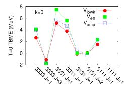
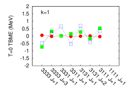
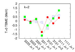
Figure 1: Matrix elements of the $p$ shell monopole-free interaction. $V_{lowk}$ potential (first order interaction) is compared to the effective Hamiltonian ($V_{eff}$) calculated in the 3rd order $\hat{Q}$-box method including folded diagrams and to the empirical fit ($V_{emp}$). Central ($k=0$), spin-orbit ($k=1$) and tensor ($k=2$) components are disentangled. $3$ stands here for the $p_{3/2}$ and $1$ for the $p_{1/2}$ orbital.

In Tables 1,2 we show the eigenvalues of multipole operators in the first ($V_{lowk}$) and third order $\hat{Q}$-box with folded diagrams ($V_{eff}$) interactions compared to the empirical fits ($V_{emp}$) in $p$ and $sd$ shells. We diagonalize separately central, spin-orbit and tensor components in each case.

Table 1: Eigenvalues of the leading multipoles in the $p$-shell. Central, spin-orbit and tensor components of the CD-Bonn potential smoothed with the $V_{lowk}$ procedure, 3rd order interaction with folded diagrams ($V_{eff}$) and the empirical fit ($V_{emp}$) are distinguished.

Multipole	Interaction	Central	Spin-orbit	Tensor	Total
$JT=10$	$V_{lowk}$	-4.46	-0.04	-1.30	-4.00
	$V_{eff}$	-6.23	-0.77	-2.17	-6.28
	$V_{emp}$	-4.11	-1.11	-1.22	-4.42
$JT=01$	$V_{lowk}$	-4.88	-0.30	-0.85	-5.72
	$V_{eff}$	-6.77	-0.20	-0.58	-7.16
	$V_{emp}$	-6.85	-0.16	-0.72	-6.83
$\lambda\tau=10$	$V_{lowk}$	-1.71	-0.44	-0.87	-1.90
	$V_{eff}$	-2.22	-0.29	-0.66	-2.59
	$V_{emp}$	-1.67	-0.48	-0.48	-2.00
$\lambda\tau=20$	$V_{lowk}$	-3.06	-0.26	-0.34	-3.05
	$V_{eff}$	-4.31	-0.16	-0.07	-4.26
	$V_{emp}$	-3.56	-0.22	-0.30	-3.59
$\lambda\tau=11$	$V_{lowk}$	2.43	0.15	0.19	2.35
	$V_{eff}$	3.51	0.21	0.17	3.49
	$V_{emp}$	2.93	0.09	0.24	2.96
$\lambda\tau=30$	$V_{lowk}$	-0.67	0.09	0.06	-0.52
	$V_{eff}$	-0.98	0.20	0.00	-0.78
	$V_{emp}$	-1.02	0.33	0.03	-0.65

Table 2: The same as in table 1 but for the $sd$ shell.

Multipole	Interaction	Central	Spin-orbit	Tensor	Total
$JT=10$	$V_{lowk}$	-4.78	-0.02	-0.98	-4.93
	$V_{eff}$	-7.24	-0.62	-2.02	-8.08
	$V_{emp}$	-5.61	-0.61	-2.03	-6.58
$JT=01$	$V_{lowk}$	-4.18	-0.02	-0.24	-4.41
	$V_{eff}$	-6.37	-0.02	-0.15	-6.38
	$V_{emp}$	-5.76	-0.13	-0.10	-5.80
$\lambda\tau=10$	$V_{lowk}$	-1.38	-0.32	-0.71	-1.53
	$V_{eff}$	-1.91	-0.19	-0.77	-2.09
	$V_{emp}$	-1.22	-0.89	-0.43	-1.66
$\lambda\tau=20$	$V_{lowk}$	-2.85	-0.31	-0.35	-2.86
	$V_{eff}$	-4.47	-0.69	-0.17	-4.54
	$V_{emp}$	-3.38	-0.52	-0.16	-3.44
$\lambda\tau=11$	$V_{lowk}$	2.77	0.10	0.24	2.75
	$V_{eff}$	4.11	0.10	0.28	4.09
	$V_{emp}$	3.81	0.28	0.31	3.85
$\lambda\tau=30$	$V_{lowk}$	-0.75	-0.23	-0.48	-0.77
	$V_{eff}$	-0.99	-0.22	-0.23	-1.10
	$V_{emp}$	-0.73	-0.23	-0.34	-1.04

Several points need to be noted from Tables 1, 2:

(i) The central parts of the multipole interactions have the eigenvalues very close to that of the total multipole Hamiltonian. A fact expected from Dufour and Zuker (1996) and supporting the operator forms proposed for the leading multipole terms.

(ii) It is interesting to notice that the eigenvalues of tensor and spin-orbit components in $JT=10$ and $\lambda\tau=10$ are the largest and these are the cases for which the weakest overlaps with the schematic operators were found in Ref. Dufour and Zuker (1996).

(iii) In-medium corrections and empirical fits affect all the multipole components in all its spin-isospin structures, though the change is of course the most visible in the largest central part. Even if the renormalization persistency of the tensor force does not hold for the multipole part, this is of minor importance for nuclear modeling. The first order tensor contribution in the multipole Hamiltonian can be simply neglected.

(iv) In the majority of cases, the fit tends to reduce the multipole component to a value somewhere in between the $V_{lowk}$ and $V_{eff}$. Roughly the eigenvalues of the empirical interaction can be obtained from $V_{lowk}$/$V_{eff}$ by multiplying/dividing its TBME by a factor 1.2 in both shells.

(v) We presented the results in $p$ and $sd$ shells only but given the properties of the multipole Hamiltonian Dufour and Zuker (1996), the analysis in any other shell or in multi-shell valence spaces could yield the same conclusions.

IV.2 Convergence of multipoles

So far, we did not discuss the cutoff and convergence properties of the multipole terms in different interactions. Examining the cutoff dependence of the calculated observables may be a useful way to estimate the uncertainty of the results due to the neglected many-body forces and the problems in the perturbative treatment. In Ref. Sieja and Nowacki (2011) we noticed that the cutoff dependence of multipoles is rather weak in the range of $1.8-2.6$fm^-1, at least for pairing and quadrupole in the $T=1$ channel. Here we repeated this analysis for all the multipoles in the wide range of $\Lambda=1.6-2.6$fm^-1. The result is shown in Fig. 2 for the multipoles of the $V_{lowk}$ potential in the $sd$-shell, distinguishing as well cutoff variation of the central, spin-orbit and tensor components. We have multiplied the value of the $\lambda\tau=11$ by -1 and skipped the $\lambda\tau=30$ for a better transparency in the Figure. The omitted octupole term shows a quite weak cutoff dependence changing its value on about $10\%$ within the examined cutoff range. As can be seen from the Figure, the $JT=10$ shows the strongest cutoff dependence. The strong cutoff dependence of the $T=0$ TBME was attributed to the contribution of the short-range tensor force. One can also note, what was already apparent from the Tables 1, 2, that the multipoles of the $V_{lowk}$ are basically given by its central component, which has the strongest variation with $\Lambda$. The negligible vector and a bit larger tensor component are nearly cutoff independent (note however different energy scales in the Figure).

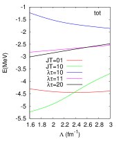
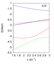
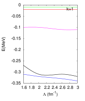
Figure 2: Multipole eigenvalues in the $V_{lowk}$ potential and its central, vector and tensor components, depending on the cutoff $\Lambda$ The value of $\lambda\tau=11$ is multiplied by -1. See text for details.

In Fig. 3 we show the convergence of multipoles of an effective Hamiltonian in the $sd$-shell, this time eigenvalues of multipoles calculated to 3rd order in $\hat{Q}$-box are plotted against the number of $\hbar\omega$ excitations permitted for intermediate diagrams, obtained with the $V_{lowk}$ potential at different cutoffs. For the lower cutoffs the multipole values are converged at 10$\hbar\omega$, a larger value is necessary for higher cutoff. As expected, with the many-body correlations included the cutoff dependence gets weaker and the monopoles converged in terms of $\hbar\omega$ are fairly the same for studied cutoffs. With the only exception of the $\lambda\tau=20$ quadrupole term, which however, as we show in the next paragraph, has a minor impact on the calculated properties of deformed nuclei.

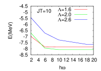
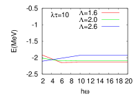
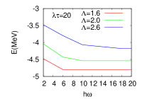
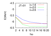
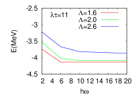
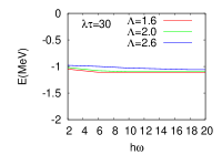
Figure 3: Multipole Hamiltonian eigenvalues plotted vs $\hbar\omega$ excitations of 2-body diagrams included in the evaluation of $\hat{Q}$-box for different cutoffs of the starting $V_{lowk}$ potential. $\lambda\tau=11$ value is multiplied by -1. Note different energy range in the case of $JT=10$.

Finally, in Tab. 3 we show the convergence of calculated multipoles in the $sd$-shell in the perturbation expansion. Tha calculation is done for the $V_{lowk}$ cutoff $\Lambda=2.0$fm^-1.

Table 3: Convergence of the eigenvalues of different multipole terms in the order-by-order perturbative expansion. $V_{lowk}$ states for the first order interaction, CP means the second-order interaction with the core-polarization contribution, 2nd-the second order interaction with all possible contributions (CP and 4p2h and ladder diagrams and folded diagrams), $\hat{Q}(2)$ is the second order $\hat{Q}$-box with folded diagrams and $\hat{Q}(3)\equiv V_{eff}$ is the 3rd order $\hat{Q}$-box interaction with folded diagrams.

Multipole	$V_{lowk}$	CP	2nd	$\hat{Q}(2)$	3rd	$\hat{Q}(3)$
$JT=10$	-4.93	-4.48	-8.23	-6.90	-10.05	-8.08
$JT=01$	-4.41	-6.31	-7.41	-6.29	-7.16	-6.38
$\lambda\tau=10$	-1.53	-2.11	-1.93	-1.71	-2.37	-2.09
$\lambda\tau=20$	-2.86	-3.43	-4.58	-3.96	-5.24	-4.54
$\lambda\tau=11$	2.75	3.15	3.80	3.35	4.68	4.09
$\lambda\tau=30$	-0.77	-1.00	-1.07	-0.94	-1.02	-1.10

A large gain in the $JT=01$ channel between the first order interaction and that including CP effects can be noticed from the Table, which improves the pairing properties obtained in the $V_{eff}$ substantially. Note, that nearly the same eigenvalue of $JT=01$ is obtained for CP, $\hat{Q}(2)$ and $\hat{Q}(3)$. Otherwise, the order-by-order convergence is far from being satisfying for all the multipole terms. A better convergence pattern is found in terms of $\hat{Q}$-boxes. As previously, the behaviour of $JT=10$ term appears the most unstable.

It is important to evoke that the conclusions we obtain here on the convergence of the multipole Hamiltonian follow exactly what has been discussed e.g. for pairing TBME derived from G-matrices in Ref. Hjorth-Jensen et al. (1995), in $sd$ and $pf$ shells. Though there are conceptual differences in the construction of the low$-k$ potentials and G-matrices, and in the resulting decoupling of high and low momenta in both methods, these differences are not much apparent in the calculations in finite nuclei. On the contrary, common problems are inherent to effective interactions derived from G-matrices and $V_{lowk}$ potentials, on both monopole Schwenk and Zuker (2006) and multipole levels.

IV.3 Multipoles and calculated observables

To realize how the possible error in the multipoles of the Hamiltonian influences the calculated observables, the following excercise was done: the monopoles of $V_{lowk}$ and $V_{eff}$ (whose multipole eigenvalues are given in Tables 1,2) were replaced by the monopoles of the corresponding $V_{emp}$. With such interactions, having exactly the same monopole fields, we have recalculated the spectra of all nuclei which were used in the empirical fits of the Hamiltonian. In the $sd$-shell we obtain the rms of 1.48MeV for $V_{lowk}$ and 1.18MeV $V_{eff}$, a very considerable deterioration from the rms=0.22MeV of the $V_{emp}$. Given that as an the intermediate step (see Sec. III) we have fitted only monopoles of $V_{eff}$ and obtained the rms error of 0.83MeV, one might conclude that the fine tuning of monopoles depends on the associated multipole and the correct multipole can be only defined within a given set of monopoles.

However, a stringent test for the pairing part of the Hamiltonian is provided by the spectra of 2 particles (2 holes) systems, in which the $0^{+}-2^{+}$ splitting should reflect the strength of the $J=0$ pairing interaction. To some extent, the quadrupole content of the interaction can be also tested by properties of deformed nuclei in a given model space. Therefore, with the same interactions (i.e. having exactly the same monopoles) we have calculated the properties of ¹⁸O, ³⁸Ar, ²⁰Ne and ²⁴Mg nuclei, which allows to visualize how the possible error in the multipole interaction influences the calculated observables.

The $2^{+}$ state of ¹⁸O, experimentally located at 1.98MeV, is of course accurately reproduced by the empirical fit (1.97MeV) while the $V_{lowk}$ places it at 1.24MeV. This anti-pairing behavior of $V_{lowk}$ is cutoff independent and also present in G-matrix interactions and taking into account the core-polarization corrections is necessary to recover the correct multipole magnitude. $V_{eff}$ does then much better in this context, leading to only a bit too high $2^{+}$ energy in ¹⁸O of 2.21MeV. In all three cases the wave function of the ground state contains $84\%$ of the $d_{5/2}^{2}$ configuration, which explains the sensivity of the calculated $2^{+}$ energy to the strength of the $d_{5/2}-d_{5/2}$ pairing interaction. Further, we have calculated the $2^{+}$ energy of ³⁸Ar. The ground state wave function in all cases contains $\sim 90\%$ of $d_{3/2}^{-2}$ component. The empirical interaction places the $2^{+}$ state at 1.86MeV (exp=2.16MeV), while the $V_{lowk}$ at a very low energy of 0.52MeV. The $V_{eff}$ interaction, including CP effects, improves the agreement with experiment substantially, with the $2^{+}$ energy at 1.62MeV. One should note here, that although the eigenvalue of the $JT=01$ is getting reduced from $V_{eff}$ to $V_{emp}$, this is not necessarily the trend of all the pairing matrix elements; apparently the $d_{3/2}-d_{3/2}$ pairing is enhanced in the fit, contrary to the case of the $f_{7/2}-f_{7/2}$ one.

In Table 4 we show the quadrupole properties of ²⁰Ne and ²⁴Mg nuclei. All the interactions give remarkably similar results, despite of differences in their quadrupole content (see Tab. 2), a priori comparable to that of the pairing part. This is a consequence of a more complex structure of deformed nuclei. Since the wave functions in this case are spread over many components, the 20% variation in the quadrupole interaction does not lead to any considerable deviations, contrary to the cases of ¹⁸O and ³⁸Ar, where pairing dominates.

Table 4: Quadrupole properties of ²⁰Ne and ²⁴Mg nuclei obtained with different interactions, see text for details.

Nucleus	Observable		$V_{lowk}$	$V_{eff}$	$V_{emp}$
20Ne	$Q(2^{+})$ (efm2)		-15.7	-15.9	-15.8
	$B(E2;2^{+}\rightarrow 0^{+})$ (e2fm4)		59.8	59.7	59.3
	$B(E2;4^{+}\rightarrow 2^{+})$ (e2fm4)		72.9	70.9	71.8
24Mg	$Q(2^{+})$ (efm2)		-18.2	-18.1	-19.2
	$B(E2;2^{+}\rightarrow 0^{+})$(e2fm4)		92.7	109.8	97.6
	$B(E2;4^{+}\rightarrow 2^{+})$(e2fm4)		127.7	143.1	133.5

V Conclusions

We have performed the spin-tensor analysis of the monopole-free effective interactions in the $p$ and $sd$ shells. We have shown that the leading (coherent) multipoles of the realistic forces are dominated by the central interaction, supporting the equivalence of multipoles extracted from realistic TBME and schematic operator forms proposed in Ref. Dufour and Zuker (1996). We have also shown that the renormalization persistency of the tensor force, observed in the $J$-averaged matrix elements, is no longer present as far as monopole-free matrix elements are concerned. However, this property of the tensor force is of a minor importance in the nuclear modeling as the contribution of the first-order tensor effects to the coherent part of the multipole Hamiltonian is negligible. Further, we have compared the $V_{lowk}$ potentials based on the CD-Bonn force to the phenomenological forces based on the same starting potential. The leading multipoles of the interactions are moderately modified in the empirical fits, as required by the ”realistic-compatibility” condition, nonetheless their modification along with the monopole part is inevitable to obtain shell-model interactions of a satisfactory precision. On average, the leading multipoles of the empirical interaction appear weaker than in the $\hat{Q}$-box effective interactions but stronger than in a realistic potential smoothed via the $V_{lowk}$ procedure with a 2fm^-1 cutoff. The convergence properties of the multipoles of the effective interactions derived here from the $V_{lowk}$ potentials are the same as those of the G-matrix based interactions from Ref. Hjorth-Jensen et al. (1995), showing again their quantitative similarity invoked in Ref. Schwenk and Zuker (2006). It would be of a great interest to investigate how the inclusion of 3-body forces would influence the couplings in the multipole Hamiltonian and wether it could explain the multipole modifications required by the fit. Some light on this issue can be shed in the nearest future, once the 2-body effective interactions with both, $T=1$ and $T=0$ effective 3-body components, are evaluated.

VI Acknowledgements

We are greatful to E. Caurier and F. Nowacki for certain numerical tools which were useful in the present study.

References

- Otsuka et al. (2010a) T. Otsuka, T. Suzuki, J. D. Holt, A. Schwenk, and Y. Akaishi, Phys. Rev. Lett. 105, 032501 (2010a).
- (2) J. D. Holt, T. Otsuka, A. Schwenk, and T. Suzuki, arXiv.1009.5984.
- Otsuka et al. (2001) T. Otsuka, M. Honma, T. Mizusaki, N. Shimizu, and Y. Utsuno, Prog. Part. Nucl. Phys. 47, 319 (2001).
- Otsuka et al. (2006) T. Otsuka, T. Matsuo, and D. Abe, Phys. Rev. Lett. 97, 162501 (2006).
- Nowacki (2007) F. Nowacki, Acta Phys. Pol. B38, 1369 (2007).
- Sieja et al. (2009) K. Sieja, F. Nowacki, K. Langanke, and G. Martinez-Pinedo, Phys. Rev. C79, 064310 (2009).
- Smirnova et al. (2010) N. Smirnova, B. Bally, K. Heyde, F. Nowacki, and K. Sieja, Phys. Lett. B686, 109 (2010).
- Otsuka et al. (2010b) T. Otsuka, T. Suzuki, M. Honma, Y. Utsuno, N. Tsunoda, K. Tsukiyama, and M. Hjorth-Jensen, Phys. Rev. Lett. 104, 012501 (2010b).
- Tsunoda et al. (2011) N. Tsunoda, T. Otsuka, K. Tsukiyama, and M. Hjorth-Jensen, Phys. Rev. C 84, 044322 (2011).
- (10) F. Nowacki, presented in Workshop on Confrontation and Convergence in Nuclear Theory, ECT* Trento, 2009.
- Kuo and Brown (1968) T. Kuo and G. Brown, Nucl. Phys. 114, 241 (1968).
- Kuo and Osnes (1990) T. Kuo and E. Osnes, Folded-Diagram Theory of the Effective Interaction in Nuclei, Atoms and Molecules (Springer-Verlag, 1990).
- Hjorth-Jensen et al. (1994) M. Hjorth-Jensen, T. Engeland, A. Holt, and E. Osnes, Phys. Rep. 242, 37 (1994).
- Hjorth-Jensen et al. (1995) M. Hjorth-Jensen, T. Kuo, and E. Osnes, Phys. Rep. 261, 125 (1995).
- Zuker (1994) A. Zuker, Nucl. Phys. A576, 65 (1994).
- Dufour and Zuker (1996) M. Dufour and A. Zuker, Phys. Rev. C54, 1641 (1996).
- Sieja and Nowacki (2011) K. Sieja and F. Nowacki, Nuclear Physics A 857, 9 (2011), ISSN 0375-9474.
- Brown and Richter (2006) B. A. Brown and W. A. Richter, Phys. Rev. C 74, 034315 (2006).
- Honma et al. (2010) M. Honma et al., Phys. Rev. C80, 064323 (2010).
- (20) A. Gniady, E. Caurier, F. Nowacki, and A. Poves, unpublished.
- Machleidt (2001) R. Machleidt, Phys. Rev. C 63, 024001 (2001).
- Bogner et al. (2003) S. Bogner, T. Kuo, and A. Schwenk, Phys. Rep. 386, 1 (2003).
- (23) M. Hjorth-Jensen, http://www.fys.uio.no/ mhjensen/.
- Schwenk and Zuker (2006) A. Schwenk and A. P. Zuker, Phys. Rev. C74, 061302 (2006).