New error estimates of Lagrange-Galerkin methods for the advection equation

Abstract

We study in this paper new developments of the Lagrange-Galerkin method for the advection equation. In the first part of the article we present a new improved error estimate of the conventional Lagrange-Galerkin method. In the second part, we introduce a new local projection stabilized Lagrange-Galerkin method, whereas in the third part we introduce and analyze a discontinuity-capturing Lagrange-Galerkin method. Also, attention has been paid to the influence of the quadrature rules on the stability and accuracy of the methods via numerical experiments.

Keywords Advection equation, Lagrange-Galerkin, finite elements, local projection stabilization,
discontinuity capturing

Mathematics Subject Classification (2010) 65M12, 65M25, 65M60, 65M50

1 Introduction

We consider the Cauchy problem for the pure advection equation

$$\left\{\begin{array}[]{l}\dfrac{\partial c}{\partial t}+\mathbf{u\cdot}\nabla c=0,\ \ x\in\mathbb{R}^{d},\ t>0,\\ \\ c(x,0)=c^{0}(x),\end{array}\right.$$ (1)

where $c:\mathbb{R}^{d}\times[0,T]\rightarrow\mathbb{R}$, $\mathbf{u}:\mathbb{R}^{d}\times[0,T]\rightarrow\mathbb{R}^{d}$ is a vector-valued function and $c^{0}(x)$ is a function of compact support defined in a domain $D_{0}\subset\mathbb{R}^{d}$. It is well known that the solution of this problem given by the method of characteristics is of the form

$$c(X\mathbf{(}\cdot\mathbf{,\ }t;t+\tau),t+\tau)=c(\cdot,t),$$

$X\mathbf{(}x\mathbf{,\ }t;t+\tau)$ being the characteristic curves of the advection equation. In this paper, we present the error analysis of three versions of the so called LG method applied to solve the Cauchy problem (1), which represent numerical realizations of the theoretical method of characteristics in the framework of $H^{1}$-conforming finite elements. The first version, denoted in this paper with the name the conventional LG method, consists basically on approximating the solution $c(x,t)$ by the $L^{2}$-projection onto the finite element space; see, for instance, [19], [17] and [15]. The conventional LG method can be viewed as a kind of high order upwind method that introduces artificial diffusion in the discrete formulation, thus providing good stability properties to the numerical solution; however, as numerical experiments show, this artificial diffusion is not high enough to suppress the oscillations that appear at discontinuities of the exact solution. In order to alleviate this problem at discontinuities and extend the stability properties, we shall study a local projection stabilized Lagrange-Galekin (LPS-LG) method and a discontinuity-capturing Lagrange-Galerkin (DC-LG) method.

In the past, several authors have obtained different estimates for the $L^{2}$-norm of the error of the conventional LG method. For example, [19] calculates an estimate of the form $O(h^{m+1}/\Delta t)$, where $m$ denotes the degree of the polynomials of the $H^{1}$-conforming finite element spaces, $h$ being the largest diameter of the elements of the spatial mesh and $\Delta t$ the size of the time step. The problem with this estimate is that for fixed $h$ the error becomes unbounded when $\Delta t\rightarrow 0$. [17] removes the $\Delta t^{-1}$ dependence from the error estimate obtaining the new estimate $O(h^{m})$, this estimate allows to prove convergence of LG method for the advection equation when $\Delta t\rightarrow 0$ independently of $h$. [15] improves the estimate of [19] calculating a new estimate $O(h^{m+1}/\Delta t^{1/2})$, which for $\Delta t=O(h)$ implies that the error of the conventional LG method is of the same order as both the streamline-diffusion (SD) method formulated in the framework of space-time finite elements continuous in space and discontinuous in time and the characteristic streamline-diffusion (CSD) method, the latter method being a version of the SD method that uses space-time meshes oriented along the characteristic curves of the advection equation. Later on, [16] calculates a new estimate of the form $O(\min(1,\left\|\mathbf{u}\right\|_{L^{\infty}(\mathbb{R}^{d})^{d}}{\Delta t}/{h})h^{m+1}/{\Delta t})$, where $\left\|\mathbf{u}\right\|_{L^{\infty}((0,T);\mathbb{R}^{d})^{d}}$ denotes the supremum norm of the velocity vector $\mathbf{u}(x,t)$; then, considering that $\left\|\mathbf{u}\right\|_{L^{\infty}(\mathbb{R}^{d})^{d}}{\Delta t}/{h}$ is the CFL number, we can say that for CFL numbers less than one, the error of LG methods is $O(h^{m})$, whereas for CFL numbers larger than one the error is $O(h^{m+1}/{\Delta t})$. Numerical examples show that the latter estimate provides a better description of the error behavior of the conventional LG method than the other estimates do. In this paper, we revisit the results of the the above mentioned authors and calculate an improved new error estimate of the form $O(\min(1,\left\|\mathbf{u}\right\|_{L^{\infty}(\mathbb{R}^{d})^{d}}{\Delta t}^{1/2}/{h})h^{m+1}/{\Delta t}^{1/2})$. Some numerical examples will support the validity of this estimate.

Local projection stabilized methods have become quite popular for advection-diffusion-reaction equations, including Navier-Stokes equations, see [1], [2], [3], [9] and [20] just to cite a few, for they are symmetric and introduce artificial diffusivity via a fluctuation operator acting on the small unresolved scales. We prove that the LPS-LG method is stable in the $L^{2}$-norm, and our error analysis shows that the error of the LPS-LG method in the mesh dependent norm (to be defined below)

$$\max_{0\leq t_{n}\leq T}\left|\left|\left|c^{n}-c_{h}^{n}\right|\right|\right|=O(h^{\beta}+\min(1,\left\|\mathbf{u}\right\|_{L^{\infty}(\mathbb{R}^{d})^{d}}{\Delta t}^{1/2}/{h})h^{m+1}/{\Delta t}^{1/2}),$$

where $\beta$ is a coefficient depending on $m$. However, despite the introduction of the artificial diffusivity, numerical tests show that the LPS-LG method may exhibit an oscillatory behavior when the solution is not sufficiently smooth.

The DC-LG method might be viewed as a version of the shock capturing CSD method [15] in which the mesh alignment along the characteristic curves and the stream diffusion mechanism of the shock capturing CSD are removed; in fact, one can consider that the DC-LG method is a reformulation, in the framework of the conventional LG method, of the residual artificial viscosity method introduced in [18]. We prove that DC-LG method is stable in the $L^{2}$-norm, regardless the degree of the finite element spaces, and also in the $L^{\infty}$-norm with linear finite elements, although numerical examples show $L^{\infty}$-norm stability with quadratic polynomials in the presence of a strong discontinuity. For solutions sufficiently smooth, we are able to prove that the error in the $L^{2}$-norm is of the form $O((h^{m+1}+C_{\varepsilon}h^{\alpha})/(\Delta t^{1/2}))$, $\alpha$ and $C_{\varepsilon}$ being positive constants.

The theoretical analysis of LG methods presented in this paper are proven under the assumption that the integrals $\int_{K}\phi_{j}(X(x,t_{n};t_{n-1}))\phi_{i}(x)dx$ , which appear in the formulation of the methods, are calculated exactly; here, $K$ is a generic element of the mesh, $\phi_{i}$ is the ith global basis function of the finite element space and $X(x,t_{n},t_{n-1})$ is the foot of the characteristic curve associated with the point $x$. Noting that the integrand is the product of two piecewise continuous polynomial functions defined on two different meshes, it may become very difficult to calculate such integrals exactly, so one has to resort to quadrature rules; but as [17] and [13] show, the quadrature rules have to be of high order because otherwise the numerical solution may become either inaccurate or unstable. Being aware of this fact, we shall test the validity of our analysis of the LG methods studied in the paper by performing some benchmark numerical tests, using symmetric Gaussian rules of different orders to assess the influence of the order of the quadrature rules on the accuracy and stability.

The paper is organized as follows. We make a short presentation of the continuous problem in Section 2, and introduce the formulation and numerical analysis of the conventional LG method for the advection equation in Section 3. Some numerical examples illustrating its performance are also reported in this section. Section 4 is devoted to the formulation, analysis and numerical performance of the LPS-LG method. The DC-LG method is introduced in Section 5, studying its stability and convergence. We also present in this section several numerical tests. Some concluding remarks are written in Section 6.

We introduce some notation about the functional spaces used in the paper. For $s\geq 0$ real and real $1\leq p\leq\infty$, $W^{s,p}(D)$ denotes the real Sobolev spaces defined on $D$ for scalar real-valued functions. $\left\|\cdot\right\|_{W^{s,p}(D)}$ and $\left|\cdot\right|_{W^{s,p}(D)}$ denote the norm and semi-norm, respectively, of $W^{s,p}(D)$. When $s=0$, $W^{0,p}(D):=L^{p}(D)$. For $p=2$, the spaces $W^{s,2}(D)$ are denoted by $H^{s}(D)$, which are real Hilbert spaces with inner product $(\cdot,\cdot)_{s}$. For $s=0$, $H^{0}(D):=L^{2}(D)$, the inner product in $L^{2}(D)$ is denoted by $(\cdot,\cdot)$. $H_{0}^{1}(D)$ is the space of functions of $H^{1}(D)$ which vanish on the boundary $\partial D$ in the sense of trace. $H^{-1}$ denotes the dual space of $H_{0}^{1}(D)$. The corresponding spaces of real vector-valued functions, $v:D\rightarrow\mathbb{R}^{d}$ are denoted by $W^{s,p}(D)^{d}:=\{v:D\rightarrow\mathbb{R}^{d}:\ v_{i}\in W^{s,p}(D),\ 1\leq i\leq d\}$. Let $X$ be a real Banach space $(X,\left\|\cdot\right\|_{X})$, if $v:(0,T)\rightarrow X$ is a strongly measurable function with values in $X$, we set $\left\|v\right\|_{L^{p}(0,t;X)}=\left(\int_{0}^{t}\left\|v(\tau)\right\|_{X}^{p}d\tau\right)^{1/p}$ for $1\leq p<\infty$, and $\left\|v\right\|_{L^{\infty}(0,t;X)}=\displaystyle\text{ess}\sup_{0<\tau\leq t}\left\|v(\tau)\right\|_{X}$; when $t=T$, we shall write, unless otherwise stated, $\left\|v\right\|_{L^{p}(X)}$. We shall also use the following discrete norms:

$$\left\|v\right\|_{l^{p}(X)}=\left(\Delta t\sum_{i=1}^{N}\left\|v(\tau_{i})\right\|_{X}^{p}\right)^{1/p}\text{, \ }\left\|v\right\|_{l^{\infty}(X)}=\max_{1\leq i\leq N}\left\|v(\tau_{i})\right\|_{X},$$

corresponding to the time discrete space $l^{p}(X)\equiv l^{p}(0,T;X)$, $1\leq p<\infty$, defined as

$$l^{p}(0,T;X):=\left\{v:(0,t_{1},t_{2},\ldots,t_{N}=T)\rightarrow X:\ \ \left\|v\right\|_{l^{p}(X)}<\infty\right\},$$

when $p=\infty$

$$l^{\infty}(0,T;X):=\left\{v:(0,t_{1},t_{2},\ldots,t_{N}=T)\rightarrow X:\ \max_{1\leq i\leq N}\left\|v(\tau_{i})\right\|_{X}<\infty\right\}.$$

Finally, we shall also use the space of continuous functions such as $C^{r}(D)$ that denotes the space of $r$-times continuously differentiable functions on $D$, when $r=0$ we write $C(D)$ instead of $C^{0}(D)$; the space $C^{r,1}(\overline{D})$, $r\geq 0$, of functions defined on the closure of $D$, $r$ -times continuously differentiable and with the $r$th derivative being Lipschitz continuous; and the space of continuous and bounded functions in time with values in $X$ denoted by $C([0,T];X)$.

Throughout this paper, $C$ will denote a generic positive constant which is independent of both the space and time discretization parameters $h$ and $\Delta t$ respectively. $C$ will have different values at different places of appearance. In many places we shall use, without making any explicit statement, the Cauchy’s inequality $ab\leq\frac{\epsilon}{2}a^{2}+\frac{1}{2\epsilon}b^{2}\ (a,\ b>0,\ \epsilon>0)$, and the discrete Gronwall inequality presented in [12].

2 The Cauchy problem for the advection equation

To introduce the LG method we consider the Cauchy problem for the first order linear hyperbolic equation

$$\left\{\begin{array}[]{l}\dfrac{\partial c}{\partial t}+\mathbf{u\cdot}\nabla c=0,\ \ x\in\mathbb{R}^{d},\ t>0,\\ \\ c(x,0)=c^{0}(x),\end{array}\right.$$ (2)

where $c:\mathbb{R}^{d}\times[0,T]\rightarrow\mathbb{R}$, $\mathbf{u}:\mathbb{R}^{d}\times[0,T]\rightarrow\mathbb{R}^{d}$ is a vector-valued function and $c^{0}(x)$ is a function of compact support defined in a domain $D_{0}\subset\mathbb{R}^{d}$. Considering the characteristics curves of the first order differential operator $D/Dt:=\partial/\partial t+\mathbf{u\cdot}\nabla$ which are the solution to the system of ordinary differential equations

$$\left\{\begin{array}[]{l}\dfrac{dX\mathbf{(}x\mathbf{,}s;t)}{dt}=\mathbf{u}(X(x,s;t),t),\\ \\ X\mathbf{(}x,s;s)=x\mathbf{,}\end{array}\right.$$ (3)

we can recast problem (2) as an ordinary differential equation along the characteristics curves, $X\mathbf{(}x\mathbf{,}s;t)$, of the form

$$\left\{\begin{array}[]{l}\dfrac{Dc}{Dt}=0\text{ ,\ \ }X\mathbf{(}x\mathbf{,}s;t)\in\mathbb{R}^{d}\text{,\ }t>0,\text{\ }\\ \\ c(X\mathbf{(}x\mathbf{,}0;0),0)=c^{0}(x\mathbf{)}.\end{array}\right.$$ (4)

Assuming that $\mathbf{u}\in C([0,T],W^{1,\infty}(\mathbb{R}^{d})^{d})$, so problem (3) has a unique solution, and $c^{0}(x)$ is sufficiently smooth, we have that the solution of (4) is then given by

$$c(X\mathbf{(\cdot,\ }t;t+\tau),t+\tau)=c(\cdot,t).$$ (5)

Concerning the solution $t\rightarrow X(x,s;t)$ to (3), the following regularity results are in order.

Lemma 1

Assume that $\mathbf{u}\in C([0,T],W^{k,\infty}(\mathbb{R}^{d})^{d})$,  $k\geq 1$.  Then for $s,\ t\in[0,T]$, there exists a unique solution $t\rightarrow X(x,s;t)\$of (3), such that $X(x,s;t)\in W^{1,\infty}(W^{k,\infty}(\mathbb{R}^{d})^{d})$. Furthermore, let the multi-index $\alpha\in N^{d}$, then for all $\alpha,$ such that $1\leq\mid\alpha\mid\leq k,$ $D^{\mathbf{\alpha}}X_{i}(x,s;t)\in C([0,T],L^{\infty}(\mathbb{R}^{d}\times[0,T]))$, $1\leq i\leq d$.

Next, we consider the mapping $\varphi_{s}^{t}:\mathbb{R}^{d}\rightarrow\mathbb{R}^{d}$, defined by $\varphi_{s}^{t}(x)=X(x,s;t)$, since $X(X(x,s;t),t;s)=x$, then it follows that the mapping $\varphi_{t}^{s}$ is the inverse of $\varphi_{s}^{t}$. The Jacobian determinant of this transformation

$$J(x,s;t)=\det\left(\frac{\partial X_{i}(x,s;t)}{\partial x_{j}}\right),\ 1\leq i,j\leq d,$$ (6)

satisfies the equation

$$\frac{\partial J(x,s;t)}{\partial t}=J(x,s;t)\mathrm{div\ }\mathbf{u(}X(x,s;t),t).$$ (7)

It is easy to see that if $C_{\mathbf{u}}:=\left\|\text{{div}}\ \mathbf{u}\right\|_{L^{\infty}(D\times(0,T))}$, then

$$\exp(-C_{\mathbf{u}}\left|s-t\right|)\leq J(x,s;t)\leq\exp(C_{\mathbf{u}}\left|s-t\right|).$$ (8)

Moreover, for $\left|t-s\right|$ sufficiently small it follows that

$$K_{1}\mid x-y\mid\leq\mid X(x,s;t)-X(y,s;t)\mid\leq K_{2}\mid x-y\mid,$$ (9)

where $K_{1}=(1-\mid s-t\mid\cdot\mid\nabla\mathbf{u}\mid_{L^{\infty}(L^{\infty}(D)^{d\times d})})$, and $K_{2}=\exp(\mid s-t\mid\cdot\mid\nabla\mathbf{u}\mid_{L^{\infty}(L^{\infty}(D)^{d\times d})})$. Here, $\mid a-b\mid$ denotes the Euclidean distance between the points $a,\ b\in\mathbb{R}^{d}$. Hereafter, for the sake of simplicity, we make the assumption $\mathrm{div\ }\mathbf{u}=0$. An important consequence of this assumption is that $J(x,s;t)=1$ almost everywhere in $\mathbb{R}$. However, we must remark that one can easily accommodate the proofs of  our results to the general case of $\mathrm{div\ }\mathbf{u}\neq 0$.

3 The conventional LG method for the advection equation

In the framework of finite elements, Douglas and Russell (1982) and Pironneau (1982) proposed the so called conventional LG method as a time marching algorithm to approximate the solution of (2).

3.1 Finite element formulation

The realization of this method requires the definition of a family of partitions $D_{h}$ in a domain $D\subset\mathbb{R}^{d}$ sufficiently large, such that given $T>0$, $D_{0}\subset\subset D$ and for all $t\in[0,T]$ we can assume that $c(x,t)=0$ on the boundary $\partial D$. The partitions $D_{h}$ generated in the closed region $\overline{D}:=D\cup\partial D$ are quasi-uniform regular and composed of $d$-simplices $K$, the boundaries of which are denoted by $\partial K$. $h_{K}$ denotes the diameter of $K$ and the mesh parameter $h:=\max_{K}h_{K}$. Moreover, we shall assume that $\mathbf{u(}x,t\mathbf{)}$ is zero on the boundary $\partial D$. To define the finite element spaces we use the reference simplex $\widehat{K}$ with vertices $\left\{\widehat{x}_{i}\right\}_{i=1}^{d+1}$, $\widehat{K}:=\left\{\widehat{x}\in\mathbb{R}^{d}:0\leq\widehat{x}_{i}\leq 1,\ 1-\sum_{i=1}^{d}\widehat{x}_{i}\geq 0\right\}$, such that for each $K\in D_{h}$ there is an invertible affine mapping $F_{K}:\widehat{K}\rightarrow K,$

$$F_{K}(\widehat{x})=\mathbf{B}_{K}\widehat{x}+\mathbf{b}_{K},\ \ \mathbf{B}_{K}\in\mathcal{L}(\mathbb{R}^{d})\ \text{and}\ \mathbf{b}_{K}\in\mathbb{R}^{d}.$$

The finite element spaces used in the formulation of the LG method are the following:

$$W_{h}:=\left\{v_{h}\in C(\overline{D}):\forall K\in D_{h},\ v_{h}\mid_{K}\in P_{m}(K)\right\},\ \text{and}\ V_{h}=H_{0}^{1}(D)\cap W_{h},$$

with

$$P_{m}(K)=\left\{p(x):\text{for }x\in K\text{, }p(x)=\widehat{p}\circ F_{K}^{-1}(x)\text{, }\widehat{p}\in P_{m}(\widehat{K})\right\},$$

where $P_{m}(\widehat{K})$ denotes the set of polynomials of degree $\leq m$ defined in $\widehat{K}$. Next, we introduce some auxiliary results concerning the approximation properties of the finite element spaces. For $0<h<h_{0}<1$, there exists a constant $c_{1}$ independent of $h$ such that for $w\in H^{q+1}(D)\cap H_{0}^{1}(D)$ and $1\leq q\leq m$,

$$\inf_{v_{h}\in V_{h}}\left\{\left\|w-v_{h}\right\|+h\left\|\nabla\left(w-v_{h}\right)\right\|\right\}\leq c_{1}h^{q+1}\left|w\right|_{H^{q+1}(D)}\text{.}$$ (10)

Since the partition $D_{h}$ is quasi-uniformly regular, the following inverse inequality holds: for all $w_{h}\in W_{h}$ and $0\leq k\leq l\leq 1$, and $1\leq p\leq q\leq\infty$, there exists a constant $c_{\mathrm{inv}}$ independent of $h$ such that,

$$\left\|w_{h}\right\|_{W^{l,q}(D)}\leq c_{\mathrm{inv}}h^{d/q-d/p+k-m}\left\|w_{h}\right\|_{W^{k,p}(D)}.$$ (11)

Let $\Pi_{h}:C(D)\rightarrow W_{h}$ be the Lagrange interpolation operator in $W_{h}$ and let $P_{h}:L^{2}(D)\rightarrow V_{h}$ be the orthogonal $L^{2}$-projector defined as

$$\left(w-P_{h}w,v_{h}\right)=0\text{ \ for all }v_{h}\in V_{h}\text{,}$$ (12)

then there are constants $c_{2}$ and $c_{3}$ independent of $h$, such that for $0\leq\sigma\leq m$, and $1\leq\gamma\leq\infty$,

$$\left\|w-P_{h}w\right\|+h\left\|\nabla(w-P_{h}w)\right\|\leq c_{2}h^{\sigma+1}\left|w\right|_{H^{\sigma+1}(D)}$$ (13)

and

$$\left\|w-\Pi_{h}w\right\|_{L^{\gamma}(D)}+h\left\|\nabla(w-\Pi_{h}w)\right\|_{L^{\gamma}(D)}\leq c_{3}h^{\sigma+1}\left|w\right|_{W^{\sigma+1,\gamma}(D)},$$ (14)

respectively [7]. It is worth noting that the estimate (14) and the inverse inequality are also valid when the domain $D$ is substituted by an element $K$. The following properties of the projector $P_{h}$ are also used in the paper:

$$P_{h}v_{h}=v_{h}\ \forall v_{h}\in V_{h},$$

and (contractiveness)

$$\left\|P_{h}v\right\|\leq\left\|v\right\|\ \forall v\in L^{2}(D).$$

Let $\mathcal{P}:=$ $0=t_{0}<t_{1}<\ldots<t_{N}=T$ be a uniform partition of step length $\Delta t$ for the interval $[0,T]$, the finite element solution of (2) at time $t_{n}$, denoted by $c_{h}^{n}\in V_{h}$, is given by

$$c_{h}^{n}=\sum_{i=1}^{N_{P}}C_{i}^{n}\phi_{i},$$

where $C_{i}^{n}:=c_{h}^{n}(x_{i})$, $x_{i}$ being the $i$th mesh-point in $D_{h}$, $N_{P}$ denotes the number of mesh-points of the partition $D_{h}$, and $\{\phi_{i}\}_{i=1}^{N_{P}}$ is the set of global basis functions of $V_{h}$. The conventional LG method calculates $c_{h}^{n}\in V_{h}$ as

$$c_{h}^{n}(x)=P_{h}c_{h}^{n-1}\circ X(x,t_{n};t_{n-1}),$$ (15)

or equivalently, for all $i=1,...,N_{P},$

$$\int_{D}c_{h}^{n}(x)\phi_{i}(x)dx=\int_{D}c_{h}^{n-1}\circ X(x,t_{n};t_{n-1})\phi_{i}(x)dx,$$ (16)

where $X(x,t_{n};t_{n-1})$ is the position at time instant $t_{n-1}$ of the point that at time instant $t_{n}$ is located at the point $x$.

Notations Let us introduce some shorthand notations in order to simplify the writing of the formulas that will appear in the article. In the sequel, we sometimes use $X^{n,n-1}$ or if confusion may arise $X^{n,n-1}(x),$ to denote $X(x,t_{n};t_{n-1})$. Also, let $a(x,t)$ be a generic function defined in $\mathbb{R}^{d}\times\left[0,T\right]$, then $a^{n}(x)$ will denote the value of $a(x,t)$ at time instant $t_{n},$ that is, $a^{n}(x)=a(x,t_{n})$, whereas $a^{\ast n-1}(x)$ denotes $a^{n-1}\circ X^{n,n-1}(x)$.

Hereafter, we assume that $h\in(0,h_{0})$ and $\Delta t\in(0,\Delta t_{0})$ with $h_{0}<1$ and $\Delta t_{0}<1$.

3.2 Analysis of the conventional LG method

We begin analyzing the $L^{2}$-norm stability of the method.

Lemma 2

For all $N\geq 1$,

$$\left\|c_{h}^{N}\right\|^{2}+\sum_{n=1}^{N}\left\|c_{h}^{n}-c_{h}^{\ast n-1}\right\|^{2}=\left\|c_{h}^{0}\right\|^{2}.$$ (17)

Proof. First of all, we show that for any function $f^{\ast n-1}(x):=f^{n-1}(X(x,t_{n},t_{n-1}))\in L^{2}(D)$

$$\left\|f^{\ast n-1}\right\|=\left\|f^{n-1}\right\|.$$ (18)

To see this is so, we make the change of variable $y=X^{n,n-1}(x)$ and recall that the Jacobian determinant of this transformation, $J(x,t_{n};t_{n-1})=1$ a.e., then

$$\int_{D}\left|f^{\ast n-1}(x)\right|^{2}dx=\int_{D}\left|f^{n-1}(X^{n,n-1}(x))\right|^{2}dx=\int_{D}\left|f^{n-1}(y)\right|^{2}J^{-1}dy=\int_{D}\left|f^{n}(y)\right|^{2}dy.$$

Now, we notice that from (15) it follows that

$$\left(c_{h}^{n}-c_{h}^{\ast n-1},c_{h}^{n}\right)=0,$$

then using the elementary relation $2(a-b,a)=a^{2}+(a-b)^{2}-b^{2},\ a,b\in\mathbb{R}$, we obtain that

$$2\left(c_{h}^{n}-c_{h}^{\ast n-1},c_{h}^{n}\right)=\left\|c_{h}^{n}\right\|^{2}+\left\|c_{h}^{n}-c_{h}^{\ast n-1}\right\|^{2}-\left\|c_{h}^{\ast n-1}\right\|^{2},$$

and by virtue of (18)

$$\left\|c_{h}^{n}\right\|^{2}+\left\|c_{h}^{n}-c_{h}^{\ast n-1}\right\|^{2}-\left\|c_{h}^{n-1}\right\|^{2}=0.$$

Summing this expression from $n=1$ up to $n=N$ it follows (17).   

Remark 3

Following [15], we can interpret the term $\sum_{n=1}^{N}\left\|c_{h}^{n}-c_{h}^{\ast n-1}\right\|^{2}$ as a measure of the numerical dissipation of conventional LG methods. It is shown there that

$$\sum_{n=1}^{N}\left\|c_{h}^{n}-c_{h}^{\ast n-1}\right\|^{2}\leq C\frac{h^{4}}{\Delta t}\sum_{n=1}^{N}\Delta t\left\|\Delta_{h}^{n-1}c_{h}^{\ast n-1}\right\|^{2},$$

where $\Delta_{h}^{n-1}:H^{1}(D)\rightarrow W_{h}^{\ast n-1}:=\left\{v_{h}^{\ast n-1}(x)=v_{h}^{n-1}(X^{n,n-1}(x)):v_{h}^{n-1}(x)\in W_{h}\right\}$ denotes the discrete Laplacian operator. When $\Delta t=h$ this amounts to adding an artificial diffusion term to the continuous advection equation of the form $Ch^{3}\Delta c$; so, for sufficiently smooth solutions such an artificial diffusion is not excessive, in particular if one compares with the usual upwind method that adds an artificial diffusion therm of the form $-Ch\Delta c$, but it may be insufficient to eliminate the oscillations when the exact solution is not smooth. To deal with the case of non smooth solutions we introduce the DC-LG method.

The remainder of this section is devoted to the analysis of the convergence. We have the following result.

Theorem 4

Let $c\in L^{\infty}(H^{m+1}(D)\cap H_{0}^{1}(D))$. Then there exists a constant $C$ independent of $\Delta t,\ h,$ and $n$, such that

$$\left\|c-c_{h}\right\|_{l^{\infty}\left(L^{2}(D)\right)}\leq\left\|e^{0}\right\|+C\min\left(1,\displaystyle\frac{\Delta t^{1/2}\left\|\mathbf{u}\right\|_{L^{\infty}(W^{1,\infty}(D)^{d}))}}{h}\right)\displaystyle\frac{h^{m+1}}{\Delta t^{1/2}}\left|c\right|_{L^{\infty}(H^{m+1}(D))}.$$ (19)

Proof. The error $e^{n}:=c^{n}-c_{h}^{n}$ can be expressed as

$$e^{n}=\left(c^{n}-P_{h}c^{n}\right)+\left(P_{h}c^{n}-c_{h}^{n}\right)\equiv\rho^{n}+\theta_{h}^{n},$$ (20)

where $\theta_{h}^{n}\in V_{h}$. Noting that $P_{h}\rho^{n}=0$, then it follows that

$$\left\|e^{n}\right\|^{2}=(\rho^{n}+\theta_{h}^{n},\rho^{n}+\theta_{h}^{n})=\left\|\rho^{n}\right\|^{2}+\left\|\theta_{h}^{n}\right\|^{2}.$$

By virtue of (13), $\rho^{n}$ satisfies the bound

$$\left\|\rho^{n}\right\|_{H^{l}(D)}\leq c_{2}h^{m+1-l}\left|c^{n}\right|_{H^{m+1}(D)}\text{\ \ }(0\leq l\leq m+1).$$ (21)

To estimate $e^{n}$ we make use of (5), which implies that $c^{n}=c^{\ast n-1}$, so that $\forall v_{h}\in V_{h}$

$$(c^{n}-c^{\ast n-1},v_{h})=0,\$$

so, subtracting (15) from this equation it results the following error equation

$$\left(e^{n}-{e}^{\ast n-1},v_{h}\right)=0,$$ (22)

where ${e}^{\ast n-1}(x)=c^{n-1}(X^{n,n-1}(x))-c_{h}^{n-1}(X^{n,n-1}(x))=\rho^{n-1}\left(X^{n,n-1}(x)\right)+\theta_{h}^{n-1}\left(X^{n,n-1}(x)\right)$. Now, we calculate an error estimate from (22). First, we notice that by virtue of (18) $\left\|e^{\ast n-1}\right\|=\left\|e^{n-1}\right\|$, so this property together with the elementary relation $2(a-b)a=a^{2}+(a-b)^{2}-b^{2}$, permits us to write

$$\left\|e^{n}\right\|^{2}+\left\|e^{n}-e^{\ast n-1}\right\|^{2}-\left\|e^{n-1}\right\|^{2}=2\left(e^{n}-e^{\ast n-1},e^{n}\right).$$ (23)

Now, one needs to estimate the term $\left(e^{n}-e^{\ast n-1},e^{n}\right)$. For this purpose, we apply the argument of [15], use (20) and set

$$(e^{n}-e^{\ast n-1},e^{n})=\left(e^{n}-e^{\ast n-1},\rho^{n}\right)+\left(e^{n}-e^{\ast n-1},\theta_{h}^{n}\right),$$

but by virtue of (22), $\left(e^{n}-e^{\ast n-1},\theta_{h}^{n}\right)=0$, then the only term we have to estimate is $\left(e^{n}-e^{\ast n-1},\rho^{n}\right)$. Thus, by the Cauchy-Schwarz inequality

$$\left(e^{n}-e^{\ast n-1},\rho^{n}\right)\leq\frac{1}{4}\left\|e^{n}-e^{\ast n-1}\right\|^{2}+\left\|\rho^{n}\right\|^{2};$$ (24)

hence, one can write that

$$2\left(e^{n}-e^{\ast n-1},e^{n}\right)\leq\displaystyle\frac{1}{2}\left\|e^{n}-e^{\ast n-1}\right\|^{2}+2\left\|\rho^{n}\right\|^{2}.$$

Using this bound on the right hand side of (23) it follows that

$$\left\|e^{n}\right\|^{2}+\frac{1}{2}\left\|e^{n}-e^{\ast n-1}\right\|^{2}-\left\|e^{n-1}\right\|^{2}\leq 2\left\|\rho^{n}\right\|^{2}.$$

From this expression, summing from $n=1$ up to $n=N$ one readily obtains that

$$\left\|e^{N}\right\|^{2}+\frac{1}{2}\sum_{n=1}^{N}\left\|e^{n}-e^{\ast n-1}\right\|^{2}\leq\frac{2T}{\Delta t}\left\|\rho\right\|_{l^{\infty}(L^{2}(D))}^{2}+\left\|e^{0}\right\|^{2}.$$

Then using (21) yields

$$\left\|c-c_{h}\right\|_{l^{\infty}\left(L^{2}(D)\right)}\leq C\displaystyle\left(\frac{h^{m+1}}{\Delta t^{1/2}}\left|c\right|_{L^{\infty}(H^{m+1}(D))}\right)+\left\|e^{0}\right\|.$$ (25)

For $\Delta t=O(h)$, the error is $O(h^{m+1/2})$, which is of the same order as the streamline-diffusion method [14] for the advection equation. However, this estimate does not allow the convergence of the method when $\Delta t\rightarrow 0$ independently of $h$. To overcome this trouble, we apply the procedure of [16] to obtain an error estimate valid for all $\Delta t$. So, substituting $e^{n}=\rho^{n}+\theta_{h}^{n}$,  and$\ e^{\ast n-1}=\rho^{\ast n-1}+\theta_{h}^{\ast n-1}$ in (22) and rearranging terms yields

$$\left(\theta_{h}^{n}-\theta_{h}^{\ast n-1},v_{h}\right)=-(\rho^{n}-\rho^{n-1},v_{h})-(\rho^{n-1}-\rho^{\ast n-1},v_{h}).$$ (26)

Letting $v_{h}=\theta_{h}^{n}$ we bound each term of this equality as follows. First, we notice that $\left\|\theta_{h}^{\ast n-1}\right\|^{2}=\left\|\theta_{h}^{n-1}\right\|^{2}$ and consequently

$$\left\|\theta_{h}^{n}\right\|^{2}+\left\|\theta_{h}^{n}-\theta_{h}^{\ast n-1}\right\|^{2}-\left\|\theta_{h}^{n-1}\right\|^{2}=2\left(\theta_{h}^{n}-\theta_{h}^{\ast n-1},\theta_{h}^{n}\right).$$

Second, since for each $n$, $P_{h}\rho^{n}=0$, then it follows that $\ (\rho^{n}-\rho^{n-1},\theta_{h}^{n})=P_{h}(\rho^{n}-\rho^{n-1})=0$. It remains to bound the term $2(\rho^{n-1}-\rho^{\ast n-1},\theta_{h}^{n})$. To do so, we notice that

$$\rho^{n-1}-\rho^{\ast n-1}=\int_{t_{n-1}}^{t_{n}}\frac{d\rho(X(x,t_{n};t),t_{n-1})}{dt}dt,$$

since $\displaystyle\frac{d\rho(X(x,t_{n};t),t_{n-1})}{dt}=\mathbf{u}(X(x,t_{n};t),t)\cdot\nabla_{X}\rho(X(x,t_{n};t),t_{n-1})$, then by the Cauchy-Schwarz inequality we get

$$\left|\rho^{n-1}-\rho^{\ast n-1}\right|^{2}\leq\Delta t\int_{t_{n-1}}^{t_{n}}\left|\mathbf{u}(X(x,t_{n};t),t)\cdot\nabla_{X}\rho(X(x,t_{n};t),t_{n-1})\right|^{2}dt,$$

so, letting $y=X(x,t_{n};t)$ and denoting by $J^{t,n}$ the Jacobian determinant $J(x,t;t_{n}):=\left(\frac{\partial X(x,t;t_{n})}{\partial x}\right)=1$, it follows that

$$\begin{array}[]{r}\left\|\rho^{n-1}-\rho^{\ast n-1}\right\|^{2}\leq\Delta t\displaystyle\int_{D}\int_{t_{n-1}}^{t_{n}}\left|\mathbf{u}(y,t)\cdot\nabla\rho^{n-1}(y)\right|^{2}\left(J^{t,n-1}\right)^{-1}dtdy\\ \\ \leq\Delta t\left\|\mathbf{u}\right\|_{L^{\infty}(L^{\infty}(D)^{d})}^{2}\displaystyle\int_{t_{n-1}}^{t_{n}}\int_{D}\left|\nabla\rho^{n-1}(y)\right|^{2}dydt\text{ }\\ \\ \leq\Delta t^{2}\left\|\mathbf{u}\right\|_{L^{\infty}(L^{\infty}(D)^{d})}^{2}\left\|\nabla\rho^{n-1}\right\|^{2}.\end{array}$$

Now, using the estimate (21) we can write that

$$\left\|\rho^{n-1}-\rho^{\ast n-1}\right\|^{2}\leq\Delta t^{2}C\left(\frac{\Delta t^{1/2}\left\|\mathbf{u}\right\|_{L^{\infty}(L^{\infty}(D)^{d})}}{h}\right)^{2}\left(\frac{h^{m+1}}{\Delta t^{1/2}}\right)^{2}\left|c\right|_{L^{\infty}(H^{m+1}(D))}^{2}.$$ (27)

Then

$$\begin{array}[]{l}2(\rho^{n-1}-\rho^{\ast n-1},\theta_{h}^{n})\leq\displaystyle\frac{2}{\Delta t}\left\|\rho^{n-1}-\rho^{\ast n-1}\right\|^{2}+\displaystyle\frac{\Delta t}{2}\left\|\theta_{h}^{n}\right\|^{2}\\ \\ \leq\Delta tC\displaystyle\left(\frac{\Delta t^{1/2}\left\|\mathbf{u}\right\|_{L^{\infty}(L^{,\infty}(D)^{d})}}{h}\right)^{2}\left(\frac{h^{m+1}}{\Delta t^{1/2}}\right)^{2}\left|c\right|_{L^{\infty}(0,T;H^{m+1}(D))}^{2}+\displaystyle\frac{\Delta t}{2}\left\|\theta_{h}^{n}\right\|^{2}.\end{array}$$

Collecting all these bounds we have that

$$\left\|\theta_{h}^{n}\right\|^{2}+\left\|\theta_{h}^{n}-\theta_{h}^{\ast n-1}\right\|^{2}-\left\|\theta_{h}^{n-1}\right\|^{2}\leq\Delta tC\displaystyle\left(\frac{\Delta t^{1/2}\left\|\mathbf{u}\right\|_{L^{\infty}(L^{\infty}(D)^{d})}}{h}\right)^{2}\left(\frac{h^{m+1}}{\Delta t^{1/2}}\right)^{2}\left|c\right|_{L^{\infty}(H^{m+1}(D))}^{2}+\frac{\Delta t}{2}\left\|\theta_{h}^{n}\right\|^{2}.$$

Now, summing from $n=1$ up to $n=N$ yields

$$\left\|\theta_{h}^{N}\right\|^{2}+\sum_{n=1}^{N}\left\|\theta_{h}^{n-1}-\theta_{h}^{\ast n-1}\right\|^{2}\leq\left\|\theta_{h}^{0}\right\|^{2}+R^{2}+\frac{\Delta t}{2}\sum_{n=1}^{N}\left\|\theta_{h}^{n}\right\|^{2},$$

where

$$R^{2}=\displaystyle C\left(\frac{\Delta t^{1/2}\left\|\mathbf{u}\right\|_{L^{\infty}(L^{\infty}(D)^{d})}}{h}\right)^{2}\left(\frac{h^{m+1}}{\Delta t^{1/2}}\right)^{2}\left|c\right|_{L^{\infty}(H^{m+1}(D))}^{2}.$$

Since $\left\|e^{N}\right\|^{2}=\left\|\rho^{N}\right\|^{2}+\left\|\theta_{h}^{N}\right\|^{2}$ and $\sum_{n=1}^{N}\left\|\theta_{h}^{n}\right\|^{2}+\left\|\rho^{N}\right\|^{2}\leq\sum_{n=1}^{N}\left\|e^{n}\right\|^{2}$, then it follows that

$$\left\|e^{N}\right\|^{2}+\sum_{n=1}^{N}\left\|\theta_{h}^{n-1}-\theta_{h}^{\ast n-1}\right\|^{2}\leq\left\|e^{0}\right\|^{2}+R^{2}+\Delta t\sum_{n=1}^{N}\left\|e^{n}\right\|^{2}.$$

Applying Gronwall inequality yields

$$\left\|c-c_{h}\right\|_{l^{\infty}\left(L^{2}(D)\right)}\leq C_{1}\left(\frac{\Delta t^{1/2}\left\|\mathbf{u}\right\|_{L^{\infty}(L^{\infty}(D)^{d})}}{h}\right)\left(\frac{h^{m+1}}{\Delta t^{1/2}}\right)\left|c\right|_{L^{\infty}(0,T;H^{m+1}(D))}+\left\|e^{0}\right\|.$$ (28)

Since (25) is valid, then combining it with (28) yields the result (19).   

3.3 Numerical test with the conventional LG method

We study the behavior of the conventional LG method considering the rotating hump problem [13]. The domain $D:=(-1,1)\times(-1,1)$, the velocity field is $\mathbf{u}=2\pi(-x_{2},x_{1})$, and the initial condition

$$c^{0}(x)=\left\{\begin{array}[]{l}\cos^{3}(\frac{3}{2}\pi r),\ \ r\leq 1/3,\\ \\ 0\ \ \ \ \ \ \ \ \ \ \ \ \ \ \text{otherwise,}\end{array}\right.$$ (29)

where $r^{2}=(x_{1}-0.5)^{2}+x_{2}^{2}$. Notice that the function $\cos^{p}(3\pi r/2)\in H^{p}(D),p\geq 1$, then $p=3$ allows enough smoothness for the optimal estimate of the error when $m=1$ and $2$. We show in Figure 1 the isolines of the $L^{2}$-projected initial condition in a mesh with mesh parameter $h=0.05$ and the cross section of the exact initial condition $c^{0}(x)$ at $x_{2}=0$.

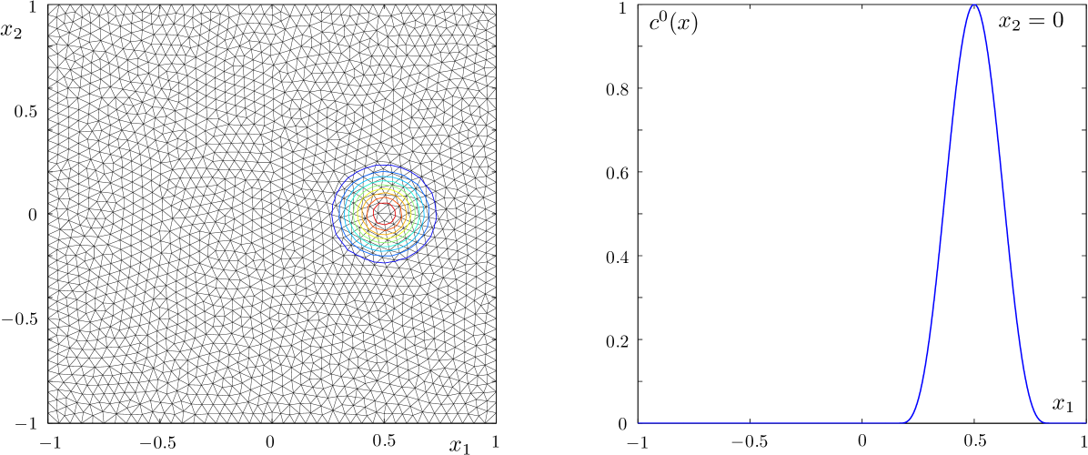
Figure 1: Initial condition of the rotating hump problem in a mesh with size $h=0.05$

The purpose of this test is to see how the error behavior fits Theorem 4. To do so, we shall mainly focus on the error as a function of the parameter $\Delta t$. Since this theorem is valid under the assumption that the integrals,

$$\int_{D}c_{h}^{n-1}\circ X^{n,n-1}(x)\phi_{i}(x)dx,$$ (30)

are calculated exactly, then we carry our goal out by using symmetric Gauss quadrature rules of different orders of accuracy to evaluate such integrals; in doing so, we assess the influence of the order of the quadrature rule on the accuracy and stability of the numerical solution.

Figure 2 shows the $L^{2}$-norm of the error as a function of the time step $\Delta t$ in two meshes with $h=0.05$ and $h=0.025$ respectively. The errors are calculated after one revolution, $T=1$, of the hump using quadrature rules for the Galerkin projection (30) of $7$, $16$, $25$, and $42$ points which are exact for polynomials of degree $5$, $8$, $10$, and $14$ respectively, see [8]. Broken lines correspond to the error function of linear polynomials ($m=1$), and full lines to the error function of quadratic polynomials ($m=2$). By inspection, we notice the following items: (a) for quadrature rules of high order, i.e., quadrature rules of 16, 25, and 42 points, there is a value $\Delta t_{s}$, such that for $\Delta t>\Delta t_{s}$, the error grows with a rate tending toward $O(\Delta t^{-1/2})$ as $\Delta t$ decreases; the error tendency of the most accurate rule of 42 points is closer to $O(\Delta t^{-1/2})$ than the error tendency of the other two rules. On the other hand, for $0<\Delta t\leq\Delta t_{s}$, the error remains almost constant and independent of $\Delta t$. (b) For quadrature rules that are not sufficiently accurate, i.e., the quadrature rule of 7 points, there is a value $\Delta t_{ins}\gg\Delta t_{s}$ at which the error starts growing very fast as $\Delta t$ decreases until it reaches a maximum or eventually the numerical solution may become extremely large at $\Delta t^{\ast}$. For $\Delta t_{s}<\Delta t<\Delta t^{\ast}$ the error decreases and when $0<\Delta t\leq\Delta t_{s}$ the error remains constant. This strange behavior of the solution for the quadrature rule of 7 points, which illustrates the dependence of the stability of the LG method upon the order of the quadrature rule, is a well known feature reported by many authors, see for instance [17]; in our tests, we note that the instability with quadratic polynomials sends the numerical solution to infinity in an interval of values of $\Delta t$, whereas for linear polynomials the numerical solution, though useless, remains bounded.

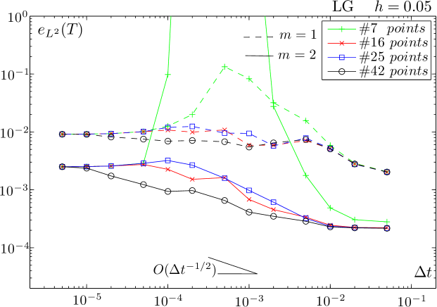
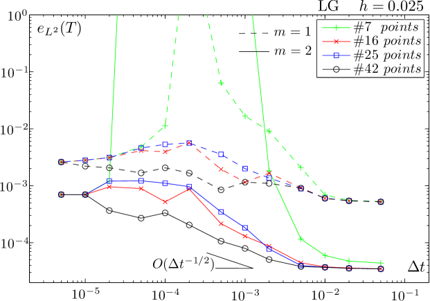
Figure 2: $L^{2}$-norm of the error of the conventional LG method in the rotating hump problem, for linear $m=1$ and quadratic $m=2$ finite elements in two different meshes ($h=0.05$ and $h=0.025$).

Other relevant results displayed in Figure 2 are the following: (c) provided that the integrals (30) are evaluated with enough accuracy, the numerical solutions are stable either for large or very small values of $\Delta t$, and as Theorem 4 says, the error is $O(h^{m+1}/{\Delta t^{1/2}})$ in the first case and $O(h^{m})$ in the second one, with the particularity that in both cases the error does not depend very much upon the order of the quadrature rule used to calculate (30) as long as such a rule is exact for polynomials of degree $>2(m+1)$. (d) The error does not grow monotonically, though we notice that the higher the order of the quadrature rule the smoother the growth of the error; however, we can not explain why the rule of order $8$ ($16$ points) gives for some values of $\Delta t$ smaller errors than the rule of order $10$ ($25$ points).

4 The LPS-LG method

To formulate the local projection stabilized Lagrange-Galerkin (LPS-LG) method we introduce additional concepts. Besides the partition $D_{h}$, we consider another quasi-uniform regular partition $\mathcal{M}_{h}$ on $D$ the elements of which are termed macro-elements. Each macro-element $M$ is decomposed into one or more elements $K$ of the partition $D_{h}$ (the case $\mathcal{M}_{h}=D_{h}$ is allowed giving place to the so-called one-level LPS approach). We assume that there exist positive constants $\gamma_{1}$ and $\gamma_{2}$ such that for all $K\subset D_{h}$ and $M\subset\mathcal{M}_{h}$, $\gamma_{1}h_{M}\leq h_{K}\leq\gamma_{2}h_{M}$. Next, we consider a discontinuous finite element space $G_{h}$ associated with $\mathcal{M}_{h}$ and set $G_{h}(M):=\left\{q_{h}\mid_{M}:q_{h}\in G_{h}\right\}$. For each $M$, we use the local $L^{2}$-projector $\pi_{M}:L^{2}(M)\rightarrow G_{h}(M)$ to define the fluctuation operator $\kappa_{M}:=id-\pi_{M}$, where $id:=L^{2}(M)\rightarrow L^{2}(M)$ is the identity operator. In addition to the approximation properties (10)-(14), we make the following assumptions.

Assumption LPS1 Let $s\in(0,\ldots,m-1)$ be the degree of the polynomials of the space $G_{h}$, the fluctuation operator $\kappa_{M}$ satisfies the approximation property

$$\left\|\kappa_{M}w\right\|_{L^{2}(M)}\leq Ch_{M}^{l}\left\|w\right\|_{H^{l}(M)},\ \forall w\in H^{l}(M),\ 0\leq l\leq s+1.$$ (31)

Let $P_{s}(M)$ be the set of polynomials of degree at most $s$ defined in $M$, then a sufficient condition for the assumption LPS1 to hold is $P_{s}(M)\subset G_{h}(M)$. We set $W_{h}(M):=\left\{w_{h}\mid_{M}:w_{h}\in W_{h},\ w_{h}=0\text{ {on\ }}D\backslash M\right\}$.

Assumption LPS2 There is an interpolation operator $j_{h}:H^{1}(D)\rightarrow W_{h}$, such that for all $(w,q_{h})\in H^{1}(D)\times G_{h}$,

$$\left(w-j_{h}w,q_{h}\right)=0,$$ (32)

and for all $w\in H^{l}(D)$, with $1\leq l\leq m+1$ and $M\in\mathcal{M}_{h}$,

$$\left\|w-j_{h}w\right\|_{L^{2}(M)}+h_{M}\left\|\nabla(w-j_{h}w)\right\|_{L^{2}(M)}\leq Ch_{M}^{l}\left\|w\right\|_{H^{l}(\Lambda(M))},$$ (33)

where $\Lambda(M)$ denotes a neighborhood of $M$.

The existence of $j_{h}$ has been proven in Part III Chapter 3 of [20] for spaces $G_{h}$ and $W_{h}$ that satisfy the following inf-sup condition :

$$\inf_{q_{h}\in G_{h}(M)}\sup_{w_{h}\in W_{h}(M)}\frac{\left(q_{h},w_{h}\right)_{M}}{\left\|q_{h}\right\|_{L^{2}(M)}\left\|w_{h}\right\|_{L^{2}(M)}}\geq\beta>0,$$

where $\beta$ is a constant independent of $h$. For simplicial meshes the spaces $(W_{h},G_{h})$ are the following (see, [20] for details):

let

$$\begin{array}[]{c}P_{m,h}^{disc}:=\{v_{h}\in L^{2}(D):v\mid_{K}=\widehat{v}\circ F_{K}^{-1}\in\widehat{P}_{m}(\widehat{K})\ \ \forall K\in D_{h}\}\ \ \mathrm{and}\\ \\ P_{m,2h}^{disc}:=\{v_{h}\in L^{2}(D):v\mid_{M}=\widehat{v}\circ F_{M}^{-1}\in\widehat{P}_{m}(\widehat{M})\ \ \forall M\in\mathcal{M}_{h}\}\text{,}\end{array}$$

where $F_{M}:\widehat{M}\rightarrow M\in\mathcal{M}_{h}$ is the bijective transformation and $\widehat{M}$ is the reference element for the partition $\mathcal{M}_{h}$. The continuous finite element space $P_{m,h}$ is defined as $P_{m,h}:=P_{m,h}^{disc}\cap H^{1}(D)$. For the one-level approach:

$$W_{h}=P_{m,h}^{+}:=P_{m,h}+\mathrm{span}_{K\in M_{h}}\{\Phi_{K}\cdot P_{m-1,h}(K)\},\ \mathrm{and}\ G_{h}=P_{m-1,h}^{disc},$$ (34)

here, $\Phi_{K}$ denotes the mapped bubble function that vanishes on the boundary $\partial K$ of the element. For the two-level approach (the elements $K\in T_{h}$ are obtained from the elements $M\in\mathcal{M}_{h}$ by means of a refinement criterium, see for instance [1] and [9]):

$$W_{h}=P_{m,h}\text{,}\ \mathrm{and}\text{ }G_{h}=P_{m-1,2h}^{disc}\text{.}$$ (35)

Figure 3 illustrates these approaches for $d=2$ and simplicial meshes.

Figure 3: Approximation and projection spaces. Left panel, the two-level approach with $m=2$; right panel, the one-level approach with $m=1$.

The LPS Lagrange-Galerkin method calculates $c_{h}^{n}\in V_{h}$ as solution of the equation

$$(c_{h}^{n}-c_{h}^{\ast n-1},v_{h})+\Delta tS_{h}(c_{h}^{n},v_{h})=0\ \ \forall v_{h}\in V_{h},$$ (36)

where $S_{h}(c_{h}^{n},v_{h})$ is the stabilization term given by the expression

$$S_{h}(c_{h}^{n},v_{h})=\sum_{M}\tau_{M}(\kappa_{M}\nabla c_{h}^{n},\kappa_{M}\nabla v_{h})_{M},$$ (37)

here, $(\kappa_{M}\nabla c_{h}^{n},\kappa_{M}\nabla v_{h})_{M}:=\int_{M}\kappa_{M}\nabla c_{h}^{n}\cdot\kappa_{M}\nabla v_{h}dx$ and $\mathbf{\tau}_{M}$ are element-wise constant coefficients that depend on the diameter $h_{M}$ of the macro-elements, their optimal values are determined by the error analysis.

Remark 5

For $v_{h}=c_{h}^{n}$ the term $S_{h}(c_{h}^{n},v_{h})$ can be written as a diffusion term of the form

$$S_{h}(c_{h}^{n},c_{h}^{n})=\sum_{M}\tau_{M}\left\|\mathbf{\kappa}_{M}\nabla c_{h}^{n}\right\|_{\mathbf{L}^{2}(M)}^{2}:=\nu_{\text{add}}(c_{h}^{n})\left\|\nabla c_{h}^{n}\right\|^{2},$$

where

$$\nu_{\text{add}}(c_{h}^{n}):=\left\{\begin{array}[]{l}\dfrac{\sum_{M}\tau_{M}\left\|\mathbf{\kappa}_{M}\nabla c_{h}^{n}\right\|_{\mathbf{L}^{2}(M)}^{2}}{\left\|\nabla c_{h}^{n}\right\|^{2}}\ \mathrm{when}\text{ }\left\|\nabla c_{h}^{n}\right\|\neq 0\text{,}\\ \\ 0\text{\ \ \ \ otherwise.}\end{array}\right..$$

4.1 Analysis of the LPS-LG method

We prove the stability of the LPS-LG method in the mesh dependent norm

$$\left|\left|\left|v^{n}\right|\right|\right|=\left(\left|\left|v^{n}\right|\right|^{2}+\Delta t\sum_{j=1}^{n}S_{h}(v^{j},v^{j})\right)^{1/2},$$ (38)

where $v^{j}\in H_{0}^{1}(D)$ $(j=1,..,n)$, $n$ being a positive integer. We have the following result.

Lemma 6

For all $N\geq 1$ it holds

$$\left|\left|\left|c_{h}^{N}\right|\right|\right|^{2}+\sum_{i=1}^{N}\left\|c_{h}^{i}-c_{h}^{\ast i-1}\right\|^{2}\leq\left\|c_{h}^{o}\right\|^{2}.$$ (39)

Proof. Let $v_{h}=c_{h}^{n}$ in (36), then it follows that

$$\left\|c_{h}^{n}\right\|^{2}+\left\|c_{h}^{n}-c_{h}^{\ast n-1}\right\|^{2}-\left\|c_{h}^{\ast n-1}\right\|^{2}+2\Delta tS_{h}(c_{h}^{n},c_{h}^{n})=0.$$

Noting that by virtue of (18), $\left\|c_{h}^{\ast n-1}\right\|^{2}=\left\|c_{h}^{n-1}\right\|^{2}$, then summing from $n=1$ up to $n=N\geq 1$ yields

$$\left\|c_{h}^{N}\right\|^{2}+\sum_{n=1}^{N}\left\|c_{h}^{n}-c_{h}^{\ast n-1}\right\|^{2}+2\Delta t\sum_{n=1}^{N}S_{h}(c_{h}^{n},c_{h}^{n})=\left\|c_{h}^{0}\right\|^{2}.$$

Hence, (39) follows.   

Next, we perform the error analysis. To do so, we again decompose the error function $e^{n}:=c^{n}-c_{h}^{n}$ as

$$e^{n}=(c^{n}-P_{h}c^{n})+(P_{h}c^{n}-c_{h}^{n})\equiv\rho^{n}+\theta_{h}^{n}.$$ (40)

First, we calculate an estimate for $\left|\left|\left|\rho^{L}\right|\right|\right|$.

Lemma 7

Let $c\in L^{\infty}(H^{m+1}(D)\cap H_{0}^{1}(D))$. Then, for all $0\leq L\leq N$. it follows that there exists a constant $C$ independent of $h$, $\Delta t$ and $L$ such that

$$\left|\left|\left|\rho^{L}\right|\right|\right|\leq C(h+\tau_{\max}^{1/2})h^{m}\left\|c\right\|_{L^{\infty}(H^{m+1}(D))},$$ (41)

where $\tau_{\max}=\max_{M\in\mathcal{M}_{h}}(\tau_{M})$.

Proof. We recall that

$$\left|\left|\left|\rho^{L}\right|\right|\right|^{2}=\left\|\rho^{L}\right\|^{2}+\Delta t\sum_{n=0}^{L}S_{h}(\rho^{n},\rho^{n}).$$

So, by virtue of (13) it follows that for all $L$ there is a constant independent of $h$, such that

$$\left\|\rho^{L}\right\|\leq Ch^{m+1}\left|c\right|_{L^{\infty}(H^{m+1}(D))}.$$

Next, we estimate the term $S_{h}(\rho^{n},\rho^{n})$. Making use of the triangle inequality, the contractiveness property of the local $L^{2}$-projector $\pi_{M}$, and (13) we obtain that

$$\begin{array}[]{r}S_{h}(\rho^{n},\rho^{n})=\sum_{M}\tau_{M}\left\|\kappa_{M}\nabla\rho^{n}\right\|_{L^{2}(M)}^{2}\leq 4\sum_{M}\tau_{M}\left\|\nabla\rho^{n}\right\|_{L^{2}(M)}^{2}\\ \\ \leq C\tau_{\max}h^{2m}\left\|c\right\|_{L^{\infty}\left(H^{m+1}(D)\right)}^{2}.\end{array}$$ (42)

Hence, collecting these two estimates the result (41) follows.   

We are ready to establish the convergence of the LPS-LG method.

Theorem 8

Under the assumptions of Theorem 4, there exists a constant $C$ independent of $h$, $\Delta t$ and $L$, such that for all $L$, $0\leq L\leq N$,

$$\max_{0\leq L\leq N}\left|\left|\left|e^{L}\right|\right|\right|\leq\left|\left|\left|e^{0}\right|\right|\right|+C_{3}\left(\tau_{\max}^{1/2}(h^{m}+h^{s+1})+h^{m+1}+\min\left(1,\frac{\Delta t^{1/2}\left\|\mathbf{u}\right\|_{L^{\infty}(L^{2}(D))}}{h}\right)\left(\frac{h^{m+1}}{\Delta t^{1/2}}\right)\right).$$ (43)

Proof. From (5) with $t=t_{n}$ and $\tau=-\Delta t$ and (36) we obtain the error equation

$$(e^{n}-e^{\ast n-1},v_{h})-\Delta tS_{h}(c_{h}^{n},v_{h})=0.$$ (44)

Noting that $c_{h}^{n}=c^{n}-e^{n}$, we recast this equation as

$$(e^{n}-e^{\ast n-1},v_{h})+\Delta tS_{h}(e^{n},v_{h})=\Delta tS_{h}(c^{n},v_{h}).$$

Next, setting $v_{h}=\theta_{h}^{n}=e^{n}-\rho^{n}$ and observing that $S_{h}(a+b,c)=S_{h}(a,c)+S_{h}(b,c)$ this equation becomes

$$\begin{array}[]{l}(e^{n}-e^{\ast n-1},e^{n})+\Delta tS_{h}(e^{n},e^{n})=(e^{n}-e^{\ast n-1},\rho^{n})\\ \\ +\Delta tS_{h}(e^{n},\rho^{n})+\Delta tS_{h}(e^{n},c^{n})-\Delta tS_{h}(c^{n},\rho^{n})\equiv\displaystyle\sum_{i=1}^{4}T_{i}\end{array}$$ (45)

We estimate the terms $T_{i}$ of (45). Applying Cauchy-Schwarz inequality we have that

$$\left|T_{1}\right|=\left|(e^{n}-e^{\ast n-1},\rho^{n})\right|\leq\frac{1}{4}\left\|e^{n}-e^{\ast n-1}\right\|^{2}+\left\|\rho^{n}\right\|^{2}.$$

To estimate $T_{2}$ we apply again Cauchy-Schwarz inequality and obtain

$$\begin{array}[]{r}\left|T_{2}\right|=\Delta t\left|S_{h}(e^{n},\rho^{n})\right|\leq\Delta t\left(S_{h}(e^{n},e^{n})\right)^{1/2}\left(S_{h}(\rho^{n},\rho^{n})\right)^{1/2}\\ \\ \leq(\delta/2)\Delta tS_{h}(e^{n},e^{n})+(2\delta)^{-1}\Delta tS_{h}(\rho^{n},\rho^{n}),\ \ 0<\delta<1.\end{array}$$

Similarly, we have that

$$\left|T_{3}\right|\leq(\delta/2)\Delta tS_{h}(e^{n},e^{n})+(2\delta)^{-1}\Delta tS_{h}(c^{n},c^{n}),$$

and

$$\left|T_{4}\right|\leq\frac{\Delta t}{2}S_{h}(c^{n},c^{n})+\frac{\Delta t}{2}S_{h}(\rho^{n},\rho^{n}).$$

Substituting these estimates in (45) with $\delta=1/2$ and noting that

$$2(e^{n}-e^{\ast n-1},e^{n})=\left\|e^{n}\right\|^{2}+\left\|e^{n}-e^{\ast n-1}\right\|^{2}-\left\|e^{n-1}\right\|^{2},$$

we obtain that

$$\begin{array}[]{r}\left\|e^{n}\right\|^{2}+\frac{1}{2}\left\|e^{n}-e^{\ast n-1}\right\|^{2}-\left\|e^{n-1}\right\|^{2}+\Delta tS_{h}(e^{n},e^{n})\\ \\ \leq 2\left\|\rho^{n}\right\|^{2}+3\Delta t\left(S_{h}(c^{n},c^{n})+S_{h}(\rho^{n},\rho^{n})\right).\end{array}$$

Summing both terms of this inequality from $n=1$ up to $n=N$ yields

$$\begin{array}[]{r}\left\|e^{N}\right\|^{2}+\frac{1}{2}\sum_{n=1}^{N}\left\|e^{n}-e^{\ast n-1}\right\|^{2}-\left\|e^{0}\right\|^{2}+\Delta t\sum_{n=1}^{N}S_{h}(e^{n},e^{n})\\ \\ \leq\sum_{n=1}^{N}\left\|\rho^{n}\right\|^{2}+5\Delta t\sum_{n=1}^{N}\left(S_{h}(c^{n},c^{n})+S_{h}(\rho^{n},\rho^{n})\right).\end{array}$$

Since for any non negative integer $n$,

$$\left\|\rho^{n}\right\|^{2}\leq Ch^{2(m+1)}\left|c\right|_{L^{\infty}(H^{m+1}(D))}^{2},$$

by virtue of assumption LPS1

$$S_{h}(c^{n},c^{n})\leq C\tau_{\max}h^{2(s+1)}\left|c\right|_{L^{\infty}(H^{s+2}(D))}^{2},$$ (46)

and observing that $\left\|\kappa_{M}\nabla\rho^{n}\right\|\leq 2\left\|\nabla\rho^{n}\right\|$ because $\pi_{M}$ is contractive, then (see (42))

$$S_{h}(\rho^{n},\rho^{n})\leq C\tau_{\max}h^{2m}\left|c\right|_{L^{\infty}(H^{m+1}(D))}^{2},$$ (47)

we have that

$$\begin{array}[]{r}\left\|e^{N}\right\|^{2}+\frac{1}{2}\sum_{n=1}^{N}\left\|e^{n}-e^{\ast n-1}\right\|^{2}-\left\|e^{0}\right\|^{2}+\Delta t\sum_{n=1}^{N}S_{h}(e^{n},e^{n})\\ \\ \leq C\left(\tau_{\max}(h^{2m}+h^{2(s+1)})+\frac{h^{2(m+1)}}{\Delta t}\right),\end{array}$$

or equivalently

$$\left|\left|\left|e^{N}\right|\right|\right|^{2}+\frac{1}{2}\sum_{n=1}^{N}\left\|e^{n}-e^{\ast n-1}\right\|^{2}\leq\left|\left\|e^{0}\right\|\right|^{2}+C\left(\tau_{\max}(h^{2m}+h^{2\left(s+1\right)})+\frac{h^{2\left(m+1\right)}}{\Delta t}\right).$$ (48)

Hence, it follows that

$$\max_{0\leq L\leq N}\left|\left|\left|e^{L}\right|\right|\right|\leq\left|\left|\left|e^{0}\right|\right|\right|+C\left(\tau_{\max}^{1/2}\left(h^{m}+h^{s+1}\right)+\frac{h^{m+1}}{\Delta t^{1/2}}\right).$$ (49)

This estimate of the error depends on $\Delta t^{-1/2}$ so that, for any fixed $h$, is invalid when $\Delta t\rightarrow 0$ because in this case the method does not converge. So, in order to get rid of the factor $\Delta t^{-1/2}$ we consider the following approach. Starting with the error equation (44) and setting

$$v_{h}=\theta_{h}^{n},\ e^{n}=\rho^{n}+\theta_{h}^{n},\ e^{\ast n-1}=\rho^{\ast n-1}+\theta_{h}^{\ast n-1}\ \mathrm{and\ }c_{h}^{n}=c^{n}-(\rho^{n}+\theta_{h}^{n}),$$

we get

$$\begin{array}[]{r}\left(\theta_{h}^{n}-\theta_{h}^{\ast n-1},\theta_{h}^{n}\right)+\Delta tS_{h}(\theta_{h}^{n},\theta_{h}^{n})=-(\rho^{n}-\rho^{\ast n-1},\theta_{h}^{n})\\ \\ +\Delta t\left(S_{h}(\rho^{n},\theta_{h}^{n})-S_{h}(c^{n},\theta_{h}^{n})\right).\end{array}$$

Now, noticing that $\rho^{n}-\rho^{\ast n-1}=\rho^{n}-\rho^{n-1}-\left(\rho^{\ast n-1}-\rho^{n-1}\right)$ and $\left(\rho^{n}-\rho^{n-1},\theta_{h}^{n}\right)=0$, we can write the above equation as

$$\begin{array}[]{l}\frac{1}{2}\left\|\theta_{h}^{n}\right\|^{2}+\frac{1}{4}\left\|\theta_{h}^{n}-\theta_{h}^{\ast n-1}\right\|^{2}-\frac{1}{2}\left\|\theta_{h}^{n-1}\right\|^{2}+\Delta tS_{h}(\theta_{h}^{n},\theta_{h}^{n})\\ \\ \leq-(\rho^{n-1}-\rho^{\ast n-1},\theta_{h}^{n})+\Delta t\left(S_{h}(\rho^{n},\theta_{h}^{n})-S_{h}(c^{n},\theta_{h}^{n})\right)\equiv\sum_{i=1}^{3}S_{i}.\end{array}$$ (50)

We bound the terms $S_{i}$ on the right hand side of (50). Thus, by the Cauchy-Schwarz inequality we have that

$$\left|S_{1}\right|\leq\frac{1}{\Delta t}\left\|\rho^{n-1}-\rho^{\ast n-1}\right\|^{2}+\frac{\Delta t}{4}\left\|\theta_{h}^{n}\right\|^{2};$$

since, see (27),

$$\frac{1}{\Delta t}\left\|\rho^{n-1}-\rho^{\ast n-1}\right\|^{2}\leq\Delta tC\left(\frac{\Delta t^{1/2}\left\|\mathbf{u}\right\|_{L^{\infty}(L^{\theta}(D))}}{h}\right)^{2}\left(\frac{h^{m+1}}{\Delta t^{1/2}}\right)^{2},$$

then

$$\left|S_{1}\right|\leq\Delta tC\left(\frac{\Delta t^{1/2}\left\|\mathbf{u}\right\|_{L^{\infty}(L^{\theta}(D))}}{h}\right)^{2}\left(\frac{h^{m+1}}{\Delta t^{1/2}}\right)^{2}+\frac{\Delta t}{4}\left\|\theta_{h}^{n}\right\|^{2}.$$ (51)

To bound the terms $S_{2}$ and $S_{3}$ we use the same technique as for the terms $T_{1}$ and $T_{2}$ above and obtain

$$\left|S_{2}\right|=\Delta t\left|S_{h}(\rho^{n},\theta_{h}^{n})\right|\leq(\delta/2)\Delta tS_{h}(\theta_{h}^{n},\theta_{h}^{n})+(2\delta)^{-1}\Delta tS_{h}(\rho^{n},\rho^{n}),$$

and

$$\left|S_{3}\right|=\Delta t\left|S_{h}(c^{n},\theta_{h}^{n})\right|\leq(\delta/2)\Delta tS_{h}(\theta_{h}^{n},\theta_{h}^{n})+(2\delta)^{-1}\Delta tS_{h}(c^{n},c^{n}).$$

Setting $\delta=1/2$ and substituting these bounds in (50) yields

$$\begin{array}[]{l}\left\|\theta_{h}^{n}\right\|^{2}+\frac{1}{2}\left\|\theta_{h}^{n}-\theta_{h}^{\ast n-1}\right\|^{2}-\left\|\theta_{h}^{n-1}\right\|^{2}+\Delta tS_{h}(\theta_{h}^{n},\theta_{h}^{n})\\ \\ \leq\Delta tC\displaystyle\left(\frac{\Delta t^{1/2}\left\|\mathbf{u}\right\|_{L^{\infty}(L^{\theta}(D))}}{h}\right)^{2}\left(\frac{h^{m}}{\Delta t^{1/2}}\right)^{2}+5\Delta t\left(S_{h}(\rho^{n},\rho^{n})\right)\\ \\ +5\Delta t\left(S_{h}(c^{n},c^{n})\right)+\displaystyle\frac{\Delta t}{2}\left\|\theta_{h}^{n}\right\|^{2}.\end{array}$$

Or equivalently, using (46) and (47),

$$\begin{array}[]{l}\left\|\theta_{h}^{n}\right\|^{2}+\frac{1}{2}\left\|\theta_{h}^{n}-\theta_{h}^{\ast n-1}\right\|^{2}-\left\|\theta_{h}^{n-1}\right\|^{2}+\Delta tS_{h}(\theta_{h}^{n},\theta_{h}^{n})\\ \\ \leq\Delta tC\left(\tau_{\max}(h^{2m}+h^{2\left(s+1\right)})+\left(\frac{\Delta t^{1/2}\left\|\mathbf{u}\right\|_{L^{\infty}(L^{\theta}(D))}}{h}\right)^{2}\left(\frac{h^{m}}{\Delta t^{1/2}}\right)^{2}\right)+\displaystyle\frac{\Delta t}{2}\left\|\theta_{h}^{n}\right\|^{2}.\end{array}$$

Summing both sides of this inequality from $n=1$ up to $n=N$ and applying Gronwall inequality we obtain that

$$\begin{array}[]{c}\left|\left|\left|\theta_{h}^{N}\right|\right|\right|^{2}+\frac{1}{2}\sum_{n=1}^{N}\left\|\theta_{h}^{n}-\theta_{h}^{\ast n-1}\right\|^{2}\leq\left\|\theta_{h}^{0}\right\|^{2}\\ \\ +C\left(\tau_{\max}(h^{2m}+h^{2\left(s+1\right)})\displaystyle\left(\frac{\Delta t^{1/2}\left\|\mathbf{u}\right\|_{L^{\infty}(L^{\theta}(D))}}{h}\right)^{2}\left(\frac{h^{m+1}}{\Delta t^{1/2}}\right)^{2}\right).\end{array}$$ (52)

Hence,

$$\left|\left|\left|\theta_{h}^{N}\right|\right|\right|\leq\left|\left|\left|\theta_{h}^{0}\right|\right|\right|+C\left(\tau_{\max}^{1/2}(h^{m}+h^{s+1})+\left(\frac{\Delta t^{1/2}\left\|\mathbf{u}\right\|_{L^{\infty}(L^{\theta}(D))}}{h}\right)\left(\frac{h^{m+1}}{\Delta t^{1/2}}\right)\right).$$ (53)

Now, noting that $\left|\left|\left|e^{N}\right|\right|\right|\leq\left|\left|\left|\theta_{h}^{N}\right|\right|\right|+\left|\left|\left|\rho^{N}\right|\right|\right|$ and

$$\left|\left|\left|\rho^{N}\right|\right|\right|\leq C(h^{m+1}+\tau_{\max}^{1/2}h^{m}),$$

it follows from (53) that

$$\left|\left|\left|e^{N}\right|\right|\right|\leq\left|\left|\left|e^{0}\right|\right|\right|+C\left(\tau_{\max}^{1/2}(h^{m}+h^{s+1})+h^{m+1}+\left(\frac{\Delta t^{1/2}\left\|\mathbf{u}\right\|_{L^{\infty}(L^{2}(D))}}{h}\right)\left(\frac{h^{m+1}}{\Delta t^{1/2}}\right)\right).$$ (54)

Thus, since both estimates (54) and (49) hold, then we can write that there exists a constant $C$ such that

$$\left|\left|\left|e^{N}\right|\right|\right|\leq\left|\left|\left|e^{0}\right|\right|\right|+C\left(\tau_{\max}^{1/2}(h^{m}+h^{s+1})+h^{m+1}+\min\left(1,\frac{\Delta t^{1/2}\left\|\mathbf{u}\right\|_{L^{\infty}(L^{2}(D))}}{h}\right)\left(\frac{h^{m+1}}{\Delta t^{1/2}}\right)\right).$$

 

4.2 Numerical tests with the LPS-LG method

We run, under the same premises, the rotating hump problem defined in Section 3.3, although the mesh is now composed of right triangles with legs of length $h=10^{-2}$. We show in the upper panel of Figure 4 the $L^{2}$-norm of the error as a function of $\Delta t$ for both the two-level LPS-LG method and the conventional LG method for a mesh size $h=\sqrt{2}\times 10^{-2}$ in both cases. In these experiments we have calculated the integrals (30) with a quadrature rule of 12 points, which is exact for polynomials of degree 6. The spaces $W_{h}$ and $G_{h}$ of the LPS-LG method are those shown in Figure 3, whereas the finite element space for the conventional LG method consists of piecewise quadratic polynomials defined on each one of the 3 triangles that compose the macro-element. We observe that the LPS-LG method is more stable than the conventional LG, because the latter goes unstable whereas the LPS-LG method remains stable when $\tau_{M}=\tau=h$ for all $M$, but it becomes unstable, with an instability region along the $\Delta t$-axis smaller than the one of the LG method, when $\tau_{M}=\tau=0.1h$ for all $M$. The lower panel of the figure shows that by increasing the order of the quadrature rule the LPS-LG method with $\tau_{M}=\tau=0.1h$ becomes stable.

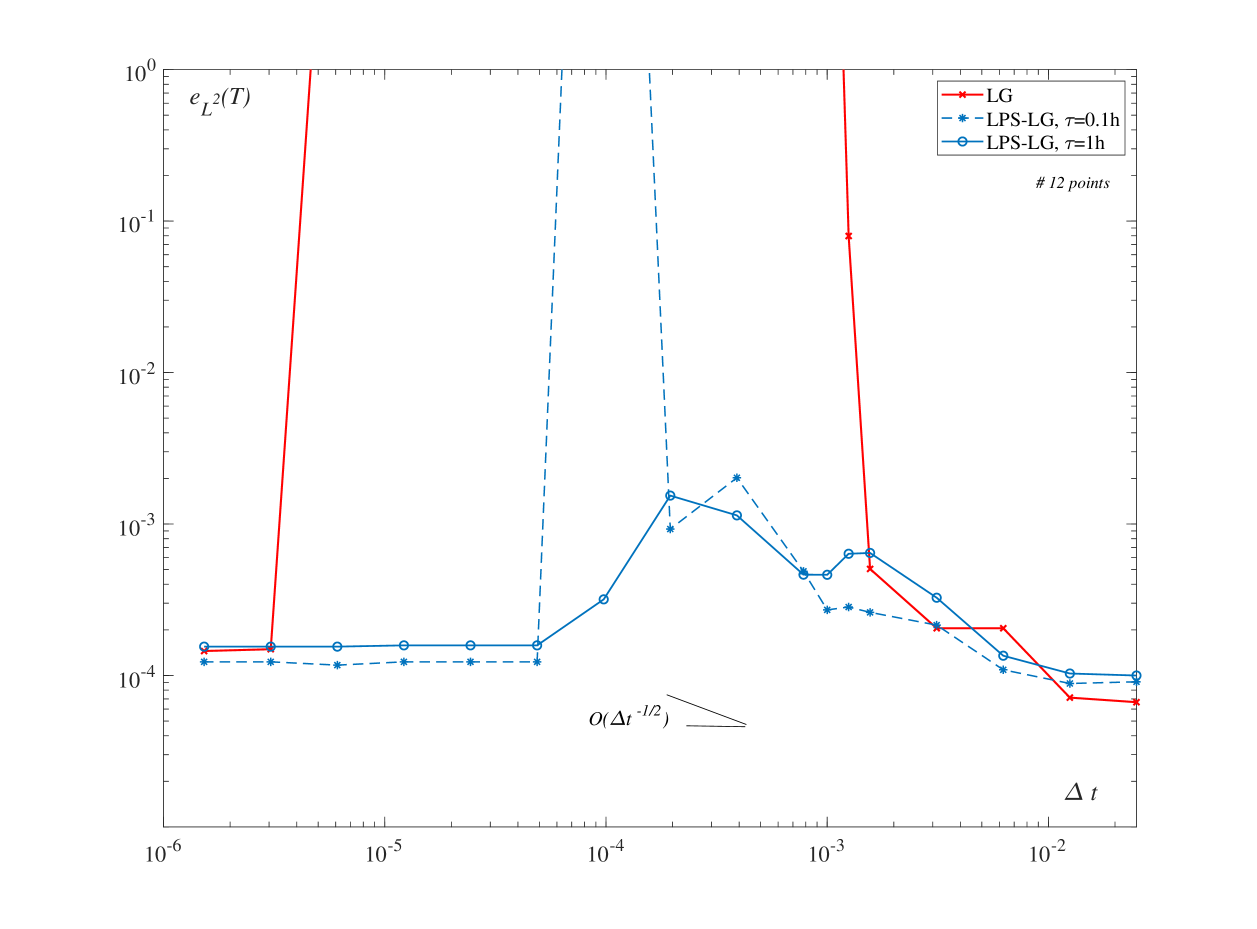
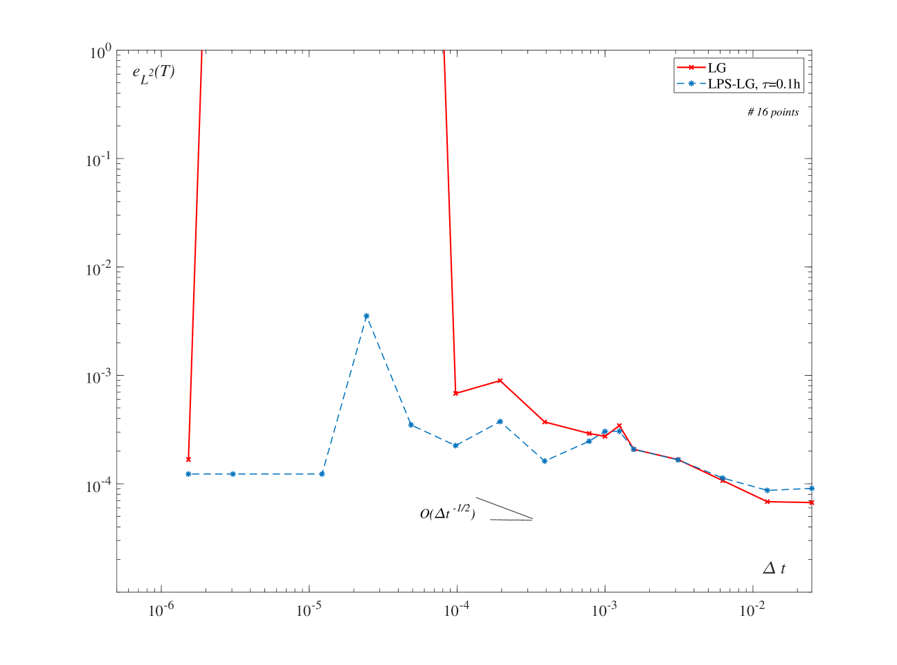
Figure 4: $L^{2}$-norm of the error in the rotating hump problem of the two-level LPS-LG method and the conventional LG method .

Figure 5 displays the $L^{2}$-norm of the error as a function of $\Delta t$ for the one level LPS-LG method, the discrete spaces of which are shown in the right panel of Figure 3, and for the conventional LG method with finite element space $W_{h}=P_{1}^{+}$. The mesh size of this experiment is $h=\sqrt{2}\times 10^{-2}$. The solid lines represent the error for the LPS-LG method with $\tau{\max}=\tau_{M}=0.1h$ and quadrature rules of $16$ and $25$ points, respectively. The dashed lines correspond to the error of the conventional LG method.

We notice in these figures that for $\Delta t=O(h)$ and $h$ such that $\min\left(1,\frac{\Delta t^{1/2}\left\|\mathbf{u}\right\|_{L^{\infty}(L^{2}(D))}}{h}\right)=1$, the solutions given by both the LPS-LG and LG methods are very similar, regardless the quadrature rule. This fact agrees with the results of Theorem 4 and Theorem 8, because in this case the dominant term of the error in the conventional LG method is $O({h^{m+1}}/{\Delta t^{1/2}})=O(h^{m+1/2})$, and in the LPS-LG method the dominant term of the error is $O({h^{m+1}}/{\Delta t^{1/2}+}\tau_{\max}^{1/2}\times(h^{m}+h^{s+1}))$, so letting $\tau_{\max}^{1/2}=ch^{1/2}$ and $s=m-1$ one has that the error is also $O(h^{m+1/2})$. However, for $\Delta t$ small enough so that $\min\left(1,\frac{\Delta t^{1/2}\left\|\mathbf{u}\right\|_{L^{\infty}(L^{2}(D))}}{h}\right)=\frac{\Delta t^{1/2}\left\|\mathbf{u}\right\|_{L^{\infty}(L^{2}(D))}}{h}$, the maximum error in the $L^{2}$-norm for the conventional LG method is $O(h^{m})$, whereas the maximum error of the LPS-LG method in the mesh dependent norm  is also $O(h^{m})$; however, since

$$\left|\left|\left|e^{N}\right|\right|\right|^{2}=\left\|e\right\|^{2}+\Delta t\sum_{n=1}^{N}\left(\sum_{M}\tau_{M}(\kappa_{M}\nabla e^{n},\kappa_{M}\nabla e^{n})_{M}\right),$$

then the $L^{2}$-error of the LPS-LG method is smaller than the $L^{2}$-error of the conventional LG method, and this is what we observe in Figure 5.

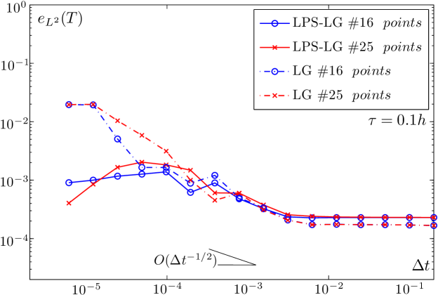
Figure 5: $L^{2}$-norm of the error in the rotating hump problem of the LPS-LG method (solid lines) and the LG method (dashed lines).

5 The DC-LG method

Numerical experiments show that when the analytical solution $c(x,t)$ is not sufficiently smooth the LG methods presented in the previous sections are not free from wiggles. Following the approach of [15], where the so called shock-capturing characteristic streamline-diffusion method is developed, but scaling the non linear dissipative term as in [18], we formulate a LG method that is stable in the maximum norm with linear finite elements, although numerical experiments show that the method may also be stable with quadratic elements; this stabilization is achieved by adding a non linear dissipative term on the left side of the formulation (16), thus obtaining the so called discontinuity-capturing LG method. In this method, we calculate $c_{h}^{n}$ as solution of

$$\left(c_{h}^{n}-c_{h}^{\ast n-1},v_{h}\right)+\Delta t\sum_{K}\left(\varepsilon_{K}(c_{h}^{n})\nabla c_{h}^{n},\nabla v_{h}\right)_{K}=0,$$ (55)

where $\left(\varepsilon_{K}(c_{h}^{n})\nabla c_{h}^{n},\nabla v_{h}\right)_{K}:=\int_{K}\varepsilon_{K}(c_{h}^{n})\nabla c_{h}^{n}\cdot\nabla v_{h}dx$ and

$$\varepsilon_{K}(c_{h}^{n}):=C_{\varepsilon}h_{K}^{\alpha}|R(c_{h}^{n})||_{K}\equiv C_{\varepsilon}h_{K}^{\alpha}\left.\frac{\left|c_{h}^{n}-c_{h}^{\ast n-1}\right|}{\Delta t}\right|_{K}.$$ (56)

Here, $C_{\varepsilon}<1$ is a user-defined positive constant, the coefficient $\alpha\in[1,2)$ and $|R(c_{h}^{n})||_{K}$ denotes the absolute value of the residual, restricted to the element $K$, generated by the discretization of the material derivative along the characteristic curves. The existence of a solution of (55) can be proven making use of Corollary 1.1 of Chapter IV of [10] as in [18]. Notice that the amount of artificial diffusion is externally controlled by $C_{\varepsilon}$, $h$ and the parameter $\alpha$, the latter must be less than 2 in order for the method to be stable in the maximum norm when the finite element space is linear.

5.1 Analysis of the DC-LG method

First, we study the stability of (55) in both the $L^{2}$ norm and the $L^{\infty}$ norm.

Lemma 9

For all $N\geq 1$, it holds

$$\left\|c_{h}^{N}\right\|^{2}+\sum_{n=1}^{N}\left\|c_{h}^{n}-c_{h}^{\ast n-1}\right\|^{2}+2\Delta t\sum_{n=1}^{N}\sum_{K}\left\|\varepsilon_{K}(c_{h}^{n})^{1/2}\nabla c_{h}^{n}\right\|_{K}^{2}\leq\left\|c_{h}^{0}\right\|^{2}.$$ (57)

Proof. Letting $v_{h}=c_{h}^{n}$ in (55) and taking into account that $\left\|c_{h}^{\ast n-1}\right\|=\left\|c_{h}^{n-1}\right\|$, it follows that

$$\left\|c_{h}^{n}\right\|^{2}+\left\|c_{h}^{n}-c_{h}^{\ast n-1}\right\|^{2}-\left\|c_{h}^{n-1}\right\|^{2}+2\Delta t\sum_{K}\left\|\varepsilon_{K}(c_{h}^{n})^{1/2}\nabla c_{h}^{n}\right\|_{K}^{2}.$$

Hence, it follows that

$$\left\|c_{h}^{N}\right\|^{2}+\sum_{n=1}^{N}\left\|c_{h}^{n}-c_{h}^{\ast n-1}\right\|^{2}+2\Delta t\sum_{n=1}^{N}\sum_{K}\left\|\varepsilon_{K}(c_{h}^{n})^{1/2}\nabla c_{h}^{n}\right\|_{K}^{2}\leq\left\|c_{h}^{0}\right\|^{2}.$$

 

Lemma 10

There is a constant $C$ independent of $h$, $\Delta t$, and $n$, but depending on the constant $C_{\varepsilon}$, such that for all $n,$

$$\left\|c_{h}^{n}\right\|_{L^{\infty}(D)}\leq(1+Ch^{\frac{1}{2}(2-\alpha)}\log(\frac{1}{h}))\left\|c_{h}^{0}\right\|_{L^{\infty}(D)}.$$ (58)

Noting that for $p\geq 1$, $\left\|c_{h}^{\ast n-1}\right\|_{L^{p}(D)}=\left\|c_{h}^{n-1}\right\|_{L^{p}(D)}$, we can prove this lemma by using the the same arguments as those employed to prove Lemma 6 in [18]. See also the proof presented in [15] of the stability in the maximum norm for the shock-capturing characteristic streamline-diffusion method. It is worth remarking that maximum norm stability has only been proven for linear finite elements, because this proof makes use of a result of [21], which says that there is a constant $c$ independent of $p=2a,\ a=1,2\ldots$, such that for all $w_{h}\in W_{h}$

$$\int_{\mathbb{R}^{d}}\nabla w_{h}\cdot\nabla\Pi_{h}(w_{h})^{p-1}dx=\frac{c}{p^{2}}\sum_{K}\int_{K}\left|\nabla w_{h}\right|\left(w_{h}\right)^{p-2}dx.$$

And this result has only been proven for linear finite elements. However, via numerical examples, we have observed that the maximum norm stability also holds in cases where the solution exhibits strong discontinuities for quadratic elements.

For the error analysis we have the following result.

Theorem 11

Let $c\in L^{\infty}(H^{m+1}(D)\cap H_{0}^{1}(D))\cap L^{\infty}(W^{1,\infty}(D))$. Then, there exists a constant $C$ independent of $\Delta t,\ h$ and $n$, but depending on $\left|D\right|$, $\left|c\right|_{L^{\infty}(H^{m+1}(D))}$ and $\left\|\nabla c\right\|_{L^{\infty}(L^{\infty}(D))}$, such that

$$\left\|c-c_{h}\right\|_{l^{\infty}\left(L^{2}(D)\right)}\leq\frac{C(h^{m+1}+C_{\varepsilon}h^{\alpha})}{\Delta t^{1/2}}.$$ (59)

Proof. The error equation is

$$\left(e^{n}-e^{\ast n-1},v_{h}\right)-\Delta t\sum_{K}(\varepsilon_{K}(c_{h}^{n})\nabla c_{h}^{n},\nabla v_{h})_{K}=0$$ (60)

Noting that $c_{h}^{n}=c^{n}-e^{n}$ we have that

$$\begin{array}[]{r}\Delta t\sum_{K}(\varepsilon_{K}(c_{h}^{n})\nabla c_{h}^{n},\nabla v_{h})_{K}=\Delta t\displaystyle\sum_{K}(\varepsilon_{K}(c_{h}^{n})\nabla c^{n},\nabla v_{h})_{K}\\ \\ -\Delta t\displaystyle\sum_{K}(\varepsilon_{K}(c_{h}^{n})\nabla e^{n},\nabla v_{h})_{K},\end{array}$$

so we can write the error equation as

$$\left(e^{n}-e^{\ast n-1},v_{h}\right)+\Delta t\sum_{K}(\varepsilon_{K}(c_{h}^{n})\nabla e^{n},\nabla v_{h})_{K}=\Delta t\sum_{K}(\varepsilon_{K}(c_{h}^{n})\nabla c^{n},\nabla v_{h})_{K}.$$ (61)

Now, setting in this equation $v_{h}=\theta_{h}^{n}=e^{n}-\rho^{n}$, where $\rho^{n}=c^{n}-$ $\Pi_{h}c^{n}$ and $\theta_{h}^{n}=\Pi_{h}c^{n}-c_{h}^{n}$, we get

$$\begin{array}[]{r}\left(e^{n}-e^{\ast n-1},e^{n}\right)+\Delta t\sum_{K}(\varepsilon_{K}(c_{h}^{n})\nabla e^{n},\nabla e^{n})_{K}=\left(e^{n}-e^{\ast n-1},\rho^{n}\right)\\ \\ +\Delta t\sum_{K}(\varepsilon_{K}(c_{h}^{n})\nabla e^{n},\nabla\rho^{n})_{K}\\ \\ +\Delta t\sum_{K}(\varepsilon_{K}(c_{h}^{n})\nabla e^{n},\nabla c^{n})_{K}\\ \\ -\Delta t\sum_{K}(\varepsilon_{K}(c_{h}^{n})\nabla c^{n},\nabla\rho^{n})_{K}\equiv\sum_{i=1}^{4}R_{i}.\end{array}$$ (62)

We estimate the terms $R_{i}$ on the right hand side. Thus, regarding $R_{1}$ we apply the Cauchy-Schwarz inequality to obtain that

$$\left|R_{1}\right|=\left|\left(e^{n}-e^{\ast n-1},\rho^{n}\right)\right|\leq\frac{1}{8}\left\|e^{n}-e^{\ast n-1}\right\|^{2}+2\left\|\rho^{n}\right\|^{2}.$$

As for the term $R_{2}$, we use the same inequality to get

$$\left|R_{2}\right|\leq(\delta/2)\Delta t\sum_{K}(\varepsilon_{K}(c_{h}^{n})\nabla e^{n},\nabla e^{n})_{K}+(2\delta)^{-1}\Delta t\sum_{K}(\varepsilon_{K}(c_{h}^{n})\nabla\rho^{n},\nabla\rho^{n})_{K},\ 0<\delta<1.$$

Similarly

$$\left|R_{3}\right|\leq(\delta/2)\Delta t\sum_{K}(\varepsilon_{K}(c_{h}^{n})\nabla e^{n},\nabla e^{n})_{K}+(2\delta)^{-1}\Delta t\sum_{K}(\varepsilon_{K}(c_{h}^{n})\nabla c^{n},\nabla c^{n})_{K},$$

and

$$\left|R_{4}\right|\leq\frac{1}{2}\Delta t\sum_{K}(\varepsilon_{K}(c_{h}^{n})\nabla c^{n},\nabla c^{n})_{K}+\frac{1}{2}\Delta t\sum_{K}(\varepsilon_{K}(c_{h}^{n})\nabla\rho^{n},\nabla\rho^{n})_{K}.$$

Substituting this estimates in (62) with $\delta=1/2$ yields

$$\begin{array}[]{r}\left\|e^{n}\right\|^{2}+\frac{3}{4}\left\|e^{n}-e^{\ast n-1}\right\|^{2}-\left\|e^{n-1}\right\|^{2}+\Delta t\sum_{K}(\varepsilon_{K}(c_{h}^{n})\nabla e^{n},\nabla e^{n})_{K}\\ \\ \leq 4\left\|\rho^{n}\right\|^{2}+3\Delta t\sum_{K}(\varepsilon_{K}(c_{h}^{n})\nabla c^{n},\nabla c^{n})_{K}\\ \\ +3\Delta t\sum_{K}(\varepsilon_{K}(c_{h}^{n})\nabla\rho^{n},\nabla\rho^{n})_{K}.\end{array}$$ (63)

Next, we have to estimate the last two terms on the right hand side of this inequality.

$$\begin{array}[]{r}\Delta t\sum_{K}(\varepsilon_{K}(c_{h}^{n})\nabla c^{n},\nabla c^{n})_{K}=C_{\varepsilon}\Delta t\displaystyle\sum_{K}h_{K}^{\alpha}\int_{K}\frac{\left|c_{h}^{n}-c_{h}^{\ast n-1}\right|}{\Delta t}\left(\nabla c^{n}\right)^{2}dK\\ \\ \leq C_{\varepsilon}\left\|\nabla c^{n}\right\|_{L^{\infty}(D)}^{2}\displaystyle\sum_{K}h_{K}^{\alpha}\int_{K}\left|c_{h}^{n}-c_{h}^{\ast n-1}\right|dK\\ \\ \leq C_{\varepsilon}\left\|\nabla c^{n}\right\|_{L^{\infty}(D)}^{2}\displaystyle\sum_{K}h_{K}^{\alpha}\left\|c_{h}^{n}-c_{h}^{\ast n-1}\right\|_{L^{1}(K)}\\ \\ \leq C_{\varepsilon}\left\|\nabla c^{n}\right\|_{L^{\infty}(D)}^{2}h^{\alpha}\left\|c_{h}^{n}-c_{h}^{\ast n-1}\right\|_{L^{1}(D)}.\end{array}$$

It remains to estimate the term $\left\|c_{h}^{n}-c_{h}^{\ast n-1}\right\|_{L^{1}(D)}$. To do so, we observe that

$$c_{h}^{n}-c_{h}^{\ast n-1}=\left(c^{n}-e^{n}\right)-\left(c^{\ast n-1}-e^{\ast n-1}\right)=e^{n}-e^{\ast n-1}$$

because $c^{n}=c^{\ast n-1}$, then $\left\|c_{h}^{n}-c_{h}^{\ast n-1}\right\|_{L^{1}(D)}=\left\|e^{n}-e^{\ast n-1}\right\|_{L^{1}(D)}$ and by virtue of the Cauchy-Schwarz inequality $\left\|e^{n}-e^{\ast n-1}\right\|_{L^{1}(D)}\leq C_{D}\left\|e^{n}-e^{\ast n-1}\right\|_{L^{2}(D)}$, $C_{D}=C(|D|)$, $|D|$ being the measure of $D$; hence

$$C_{\varepsilon}\left\|\nabla c^{n}\right\|_{L^{\infty}(D)}^{1}h^{\alpha}\left\|c_{h}^{n}-c_{h}^{\ast n-1}\right\|_{L^{1}(D)}\leq\frac{1}{16}\left\|e^{n}-e^{\ast n-1}\right\|_{L^{2}(D)}^{2}+4C_{\varepsilon}^{2}h^{2\alpha}C_{D}^{2}\left\|\nabla c^{n}\right\|_{L^{\infty}(D)}^{4}.$$

Therefore, we can set that

$$\Delta t\sum_{K}(\varepsilon_{K}(c_{h}^{n})\nabla c^{n},\nabla c^{n})_{K}\leq\frac{1}{16}\left\|e^{n}-e^{\ast n-1}\right\|_{L^{2}(D)}^{2}+4C_{\varepsilon}^{2}h^{2\alpha}C_{D}^{2}\left\|\nabla c^{n}\right\|_{L^{\infty}(D)}^{4}.$$ (64)

We estimate now the term $\Delta t\sum_{K}(\varepsilon_{K}(c_{h}^{n})\nabla\rho^{n},\nabla\rho^{n})_{K}$. To this end, we notice that

$$\Delta t\sum_{K}(\varepsilon_{K}(c_{h}^{n})\nabla\rho^{n},\nabla\rho^{n})_{K}=C_{\varepsilon}\sum_{K}h_{K}^{\alpha}\int_{K}\left|c_{h}^{n}-c_{h}^{\ast n-1}\right|\left(\nabla\rho^{n}\right)^{2}dK,$$

but by virtue of (14) we have that $\left\|\nabla\rho^{n}\right\|_{L^{\infty}(D)}\leq c_{3}\left\|\nabla c^{n}\right\|_{L^{\infty}(D)}$, then we can write that

$$\Delta t\sum_{K}(\varepsilon_{K}(c_{h}^{n})\nabla\rho^{n},\nabla\rho^{n})_{K}\leq c_{3}^{2}C_{\varepsilon}\left\|\nabla c^{n}\right\|_{L^{\infty}(D)}^{2}\sum_{K}h_{K}^{\alpha}\int_{K}\left|c_{h}^{n}-c_{h}^{\ast n-1}\right|dK;$$

so, arguing as we have just done for the term $\Delta t\sum_{K}(\varepsilon_{K}(c_{h}^{n})\nabla c^{n},\nabla c^{n})_{K}$ it follows that

$$\Delta t\sum_{K}(\varepsilon_{K}(c_{h}^{n})\nabla\rho^{n},\nabla\rho^{n})_{K}\leq\frac{1}{16}\left\|e^{n}-e^{\ast n-1}\right\|_{L^{2}(D)}^{2}+4c_{3}^{4}C_{\varepsilon}^{2}h^{2\alpha}C_{D}^{2}\left\|\nabla c^{n}\right\|_{L^{\infty}(D)}^{4}.$$ (65)

Substituting (64) and (65) in (63) and using the estimate (14) yields

$$\begin{array}[]{r}\left\|e^{n}\right\|^{2}+\frac{1}{2}\left\|e^{n}-e^{\ast n-1}\right\|^{2}-\left\|e^{n-1}\right\|^{2}+\Delta t\sum_{K}(\varepsilon_{K}(c_{h}^{n})\nabla e^{n},\nabla e^{n})_{K}\\ \\ \leq C\left(h^{2(m+1)}+C_{\varepsilon}^{2}h^{2\alpha}\right).\end{array}$$

where $C$ is a constant that depends on $C_{D}$, $\left|c^{n}\right|_{H^{m+1}(D)}$ and $\left\|\nabla c^{n}\right\|_{L^{\infty}(D)}$. Summing both terms of this inequality from $n=1$ up to $n=N$ it follows that

$$\begin{array}[]{r}\left\|e^{N}\right\|^{2}+\frac{1}{2}\sum_{n=1}^{N}\left\|e^{n}-e^{\ast n-1}\right\|^{2}+\Delta t\sum_{n=1}^{N}\sum_{K}(\varepsilon_{K}(c_{h}^{n})\nabla e^{n},\nabla e^{n})_{K}\\ \\ \leq\frac{C}{\Delta t}\left(h^{2(m+1)}+C_{\varepsilon}^{2}h^{2\alpha}\right),\end{array}$$

or equivalently

$$\left\|e^{N}\right\|\leq C\frac{\left(h^{m+1}+C_{\varepsilon}h^{\alpha}\right)}{\Delta t^{1/2}}.$$

 

Remark 12

This estimate depends on $\Delta t^{-1/2}$ so that for $h$ fixed blows up as $\Delta t\rightarrow 0$. In contrast with the previous LG methods, for the DC-LG method we have not been able to find an error estimate free from the $\Delta t^{-1/2}$ dependence; however, based on numerical experiments and assuming that the maximum norm stability holds, we may hypothesizes that there is a $\Delta t_{c}$, such that for $\Delta t\leq\Delta t_{c}$ the error will not increase, remaining nearly constant or decreasing very slowly. So, noting that $c_{h}^{n}-c_{h}^{\ast n-1}=e^{n}-e^{\ast n-1}$ because $c^{n}=c^{\ast n-1}$, we can argue that for $\Delta t\leq\Delta t_{c}$

$$\max_{n}\max_{K}\left.\frac{\left|e^{n}-e^{\ast n-1}\right|}{\Delta t}\right|_{K}=\beta,$$

$\beta$ being a small constant that depends on $m$; hence, we can consider that $\varepsilon_{K}(c_{h}^{n})$ is a constant, specifically, for all $K$ and $n$ we set

$$\nu:=\varepsilon_{K}(c_{h}^{n})=C_{\varepsilon}\beta h^{\alpha}.$$

Then, the error equation can be written now as

$$\left(e^{n}-e^{\ast n-1},v_{h}\right)-\Delta t\nu\sum_{K}(\nabla c_{h}^{n},\nabla v_{h})_{K}=0.$$ (66)

So, as we have done above, we let

$$v_{h}=\theta_{h}^{n},\ e^{n}=\rho^{n}+\theta_{h}^{n},\ e^{\ast n-1}=\rho^{\ast n-1}+\theta_{h}^{\ast n-1}\ \mathrm{and\ }c_{h}^{n}=c^{n}-(\rho^{n}+\theta_{h}^{n}),$$

with $\rho^{n}=c^{n}-P_{h}c^{n}$, and recast (66) as

$$\begin{array}[]{r}\left(\theta_{h}^{n}-\theta_{h}^{\ast n-1},\theta_{h}^{n}\right)+\Delta t\nu\nabla\theta_{h}^{n},\nabla\theta_{h}^{n})=-(\rho^{n}-\rho^{\ast n-1},\theta_{h}^{n})\\ \\ -\Delta t\nu(\nabla\rho^{n},\nabla\theta_{h}^{n})+\Delta t\nu(\nabla c^{n},\nabla\theta_{h}^{n}).\end{array}$$ (67)

If we compares this equation with (26), we can consider that the artificial dissipation terms represent a perturbation to the equation of the pure advection problem, so, we can expect that when $\nu\rightarrow 0$ (67) will yield the same estimate as (26). To check that this is the case, we bound the terms $-(\rho^{n}-\rho^{\ast n-1},\theta_{h}^{n})$, $(\nabla\rho^{n},\nabla\theta_{h}^{n})$ and $(\nabla c^{n},\nabla\theta_{h}^{n})$ as we have done many times before and can easily arrive to the estimate

$$\left\|\theta_{h}^{N}\right\|\leq C\left(h^{m}+\nu^{1/2}\right),$$

where the constant  $C$ depends on $\left|c\right|_{L^{\infty}(0,T;H^{m+1}(D))}$, and consequently,

$$\left\|e^{N}\right\|=O\left(h^{m}+\left(C_{\varepsilon}\beta h^{\alpha}\right)^{1/2}\right).$$

So, if $C_{\varepsilon}\beta$ is so small that $\left(C_{\varepsilon}\beta h^{\alpha}\right)^{1/2}\leq h^{m}$, then $\left\|e^{N}\right\|=O(h^{m})$.

5.2 Numerical tests with the DC-LG method

Since the method is designed to deal with discontinuous initial conditions, we shall perform two numerical tests. The first one is again the hump problem to see wether the error behaves according to Theorem 11; the second test uses as initial condition the so called “slotted” cylinder, this a typical initial condition to study the ability of schemes to deal with strong discontinuities.

5.2.1 The hump test

We run the test under the same conditions as the numerical test for the conventional LG method. We show in Figures 6 and 7 the results for the meshes with mesh parameter $h=0.05$ and $h=0.025$ after one revolution, and with the constants $C_{\varepsilon}$ and $\alpha$ of the expression for the artificial diffusivity (56) taking the values $C_{\varepsilon}=0.01$, $C_{\varepsilon}=0.1$ and $\alpha=\frac{3}{2}$. These results must be compared with those of Figure 2.

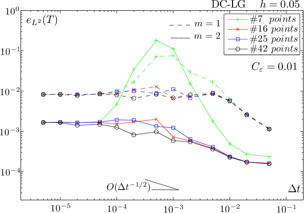
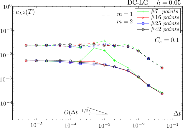
Figure 6: $L^{2}$-error norm with the DC-LG method in the rotating hump problem for $h=0.05$

We notice the following facts: (a) For high order quadrature rules, the error of the DC-LG method shows a similar, but smoother, behavior as the error of the conventional LG method, with the feature that the higher the constant $C_{\varepsilon}$ or the coarser the mesh the smoother the profile of the error curves; this is a consequence of the nonlinear artificial diffusivity that depends on both $C_{\varepsilon}$ and $h$. (b) For the low order quadrature rule of 7 points, the DC-LG method loses accuracy for those values $\Delta t$ for which the conventional LG method is inaccurate or even unstable; in fact, for $C_{\varepsilon}=0.01$ and $h=0.025$ there is an interval of values $\Delta t$, which, roughly speaking, corresponds with those values for which the conventional LG method with quadratic polynomials becomes unstable, in which the DC-LG method with quadratic polynomials is less accurate than with linear polynomials. This can be explained because when both $C_{\varepsilon}$ and $h$ are low the artificial diffusivity is not sufficiently strong to prevent the instability. (c) Roughly speaking, we can say that the higher the artificial viscosity the less sensitive the DC-LG method is to the order of the quadrature rules, provided that such rules are exact for polynomials of degree $2m$. (d) For $\Delta t=O(h)$ or $\Delta t=o(h^{2})$, all the quadrature rules give about the same solution. This means that in those ranges of values $\Delta t$ it is not necessary the use of high order quadrature rules, just a rule which is exact for polynomials of degree $2(m+1)$ would suffice. (e) Looking at the profiles of the error curves, we notice that for high order quadrature rules the error behaves as Theorem 11 says, that is, there is a value $\Delta t_{c}$ (in this test, $\Delta t_{c}=O(h^{-2})$), such that for $\Delta t\geq\Delta t_{c}$ the error is $O(h^{m+1}+C_{\varepsilon}h^{\alpha})/\Delta t^{1/2}$. However, for $\Delta t<\Delta t_{c}$, the error does not grow and remains more or less constant, particularly as the artificial diffusivity is high enough, see Figure 6. Finally, fixing the mesh and the parameter $\alpha$, this test shows that as the constant $C_{\varepsilon}$ becomes smaller and smaller, the DC-LG solution approaches the solution of conventional LG method.

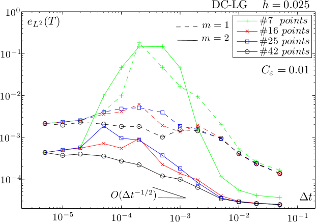
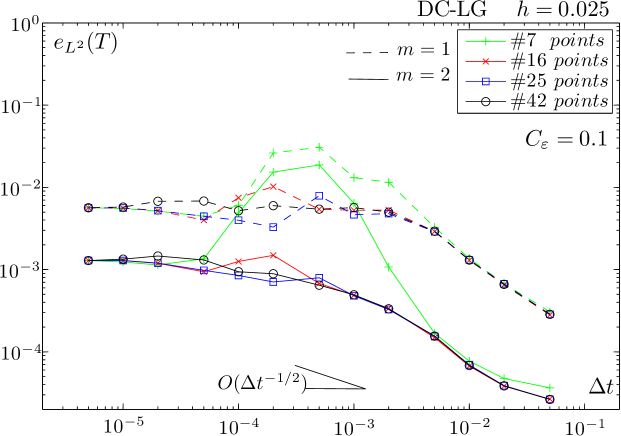
Figure 7: $L^{2}$-error norm with the DC-LG method in the rotating hump problem for $h=0.025$

5.2.2 The slotted cylinder

Our second test is the so called slotted cylinder. The idea behind this test is to assess the ability of the DC-LG method to deal with strong discontinuities; specifically, we wish to see how the scheme smears out an initial condition that is strongly discontinuous. The domain $D:=[-1,1]\times[-1,1]$, the velocity field $\mathbf{u}$ is the same as in the previous tests, i.e., $\mathbf{u}=2\pi(-x_{2},x_{1})$, and the initial condition is a cylinder of height 1 and radius 0.25 centered at (0.5,0), with a slot along the plane $x=0.5$ of width 0.1 and depth 0.35. The simulations are carried out with a time step $\Delta t=0.01$ in the mesh with mesh parameter $h=0.025$, and the numerical initial condition being computed by the $L^{2}$-projection onto the finite element space $V_{h}$. Although we are aware that this is not a good way to calculate the numerical initial condition because, as we see in Figure 9, some overshoots and undershoots are generated by the $L^{2}$-projection, we have left it to test the capability of DC-LG method to suppress the wiggles; it is clear that the method is able to kill them out after few time steps when the constant $C_{\varepsilon}$ of the artificial diffusion $\varepsilon_{h}(c_{h}^{n})$ is $C_{\varepsilon}=0.1$. A better approach to calculate the numerical initial condition would have been to perform $L^{2}$-projection of the exact initial condition with linear elements and lumped mass matrix, yielding this way a somewhat smoother initial condition. The integration time $T=1$. For the results, we have used the exact trajectories and the integrals (30) have been calculated with the quadrature rule of 16 points. Based on the results of the hump test, we know that for the values $\Delta t=0.01$ and $h=0.025$ the solution is not sensitive to the order of the quadrature rules used to approximate the integrals (30), provided that the rule is exact for polynomials of degree $>2(m+1)$.

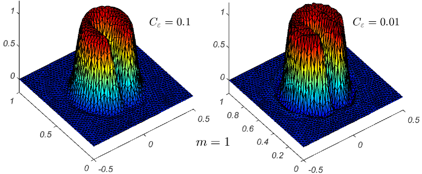
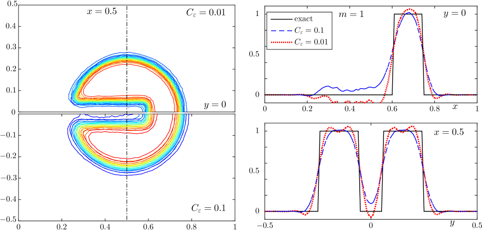
Figure 8: Slotted cylinder after one revolution for linear finite elements $m=1$. Upper panel: three dimensional view of the solutions. Lower panel: the level lines (on the left) and cross sections (on the right) that correspond with the figures of the upper panel.

We display in the upper panel of Figure 8 a three dimensional view of the cylinder after one revolution, whereas in the low panel are represented the level lines (on the left) and cross sections (on the right) when the constant of the artificial diffusion takes the values $C_{\varepsilon}=0.1$ and $C_{\varepsilon}=0.01$. This solution has been calculated with linear polynomials ($m=1$). We notice that the width of the upper face of the lobes and the width of the “bridge” as well as the depth of the slot are reasonably well preserved for both constants $C_{\varepsilon}=0.1$ and $C_{\varepsilon}=0.01$. It is worth remarking that the figures of the upper and middle panel with $C_{\varepsilon}=0.1$ compare very well with those obtained in [15] and [11] applying the shock-capturing streamline-diffusion method with a time step $\Delta t=0.01$ and the mesh size $h=0.01$, which is $2.5$ times smaller than the one we use. It is clear that with the constant $C_{\varepsilon}=0.1$ the DC-LG method introduces a major degree of smearing, and when $C_{\varepsilon}=0.01$ the method is not able to suppress the wiggles generated around the discontinuities at the first time step.

Similar representations of the numerical solution calculated with quadratic polynomials (m=2) are displayed in Figure 9. If we compare these graphs with those of Figure 8 one sees that it is clear the improvement of the numerical solution calculated with quadratic polynomials; for instance, the slopes of the cylinder sides, the width of the lobes of the upper face and the width of the “bridge” are much better represented with quadratic elements than with linear elements.

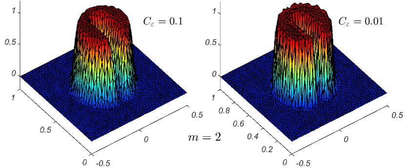
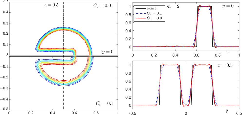
Figure 9: Slotted cylinder after one revolution for quadratic finite elements $m=2$. Upper panel: three dimensional view of the solutions. Lower panel: the level lines (on the left) and cross sections (on the right) that correspond with the figures of the upper panel.

Finally, we represent in Figure 10 the time evolution of the maximum and minimum of the numerical solutions obtained by the conventional LG method, and the DC-LG one (with $C_{\varepsilon}=0.01$ and $C_{\varepsilon}=0.1$). As we commented above, our calculation of the numerical initial condition allows the generation of wiggles at the first time step, in fact, the largest amplitude of such wiggles is $0.3$. The DC-LG method with $C_{\varepsilon}=0.1$ dissipates these wiggles as the solution progresses, such that the for $m=2$ the dissipation is very strong at the beginning, going very quickly the minimum to zero and the maximum to 1, as, on the other hand, should be; however, when $C_{\varepsilon}=0.01$, the wiggles are also dissipated, but at a slower rate, with the amplitudes of the minimum and maximum values decreasing somewhat oscillatorily, tending to $-0.05$ and $1.05$ respectively. However, though we proof that linear polynomials are stable in the maximum norm, the behavior of the maximum and minimum is not as good as that of quadratic elements; for instance, when $C_{\varepsilon}=0.1$ the dissipation of the amplitude of the wiggles is slower and less strong than in the case of quadratic elements, noting that the steady maximum and minimum are $1.03$ and $-0.03$ respectively; when $C_{\varepsilon}=0.01$ the maximum and minimum of DC-LG solution, though smaller in amplitude, exhibit a similar oscillatory behavior as those of the conventional LG method. It is remarkable that both the maximum and the minimum of the conventional LG method, either with $m=1$ or $m=2$, undergo dissipation at the beginning of the calculations and then go on exhibiting an oscillatory behavior.

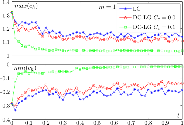
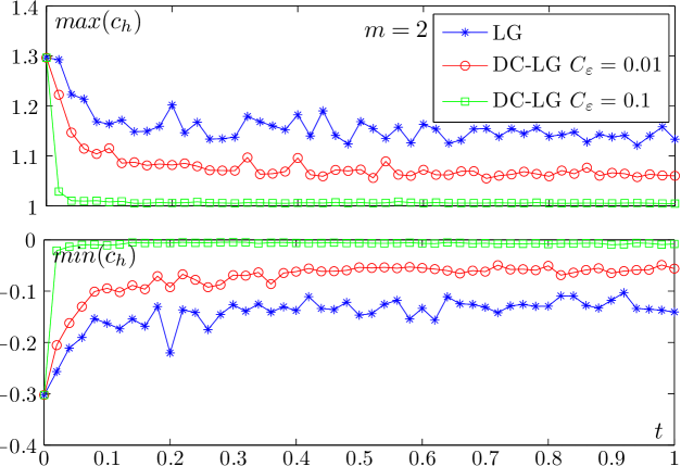
Figure 10: Evolution with time of the maximum and minimum of the slotted cylinder during one revolution for linear $m=1$ and quadratic $m=2$ finite elements

6 Concluding remarks

1) We have obtained a new error estimate of the conventional LG method for the advection equation. In contrast with previous estimates, ours is valid for all $\Delta t$, no matter how small $\Delta t$ is, showing that for $\Delta t\leq Kh^{p},\ p>2$, the error is $O(h^{m})$, and for $\Delta t>Kh^{p}$ the error is $O({h^{m+1}}/{\Delta t^{1/2}})$, here $K=(\left\|\mathbf{u}\right\|_{L^{\infty}(L^{\infty}(D)^{d})})^{-1/2}$. This error estimate has been obtained under the assumption that the integrals $\int_{K}\phi_{j}(X_{h}(x,t_{n+1},t_{n}))\phi_{i}(x)dx$ are calculated exactly. 2) To validate our theoretical result we perform numerical tests using quadrature rules of different orders to evaluate those integrals and calculating exactly the trajectories. We find that the higher the order of the quadrature rule the closer the error behavior to the theoretical one. Other interesting finding is that for $\Delta t=O(h)$ and $\Delta t=O(h^{3})$, the error is quite independent of the order of the quadrature rule as long as the rule calculates exactly polynomials of degree $\geq 2(m+1)$. 3) The LG approach is a natural way of introducing upwinding in the numerical method, but the degree of upwinding is not strong enough if the initial condition lacks regularity. One way of stabilizing the conventional LG method is using the so called local projection stabilization technique, which is symmetric and acts on the small unresolved scales. We thus obtain the so called LPS-LG method and estimate its error in a mesh dependent norm. 4) Neither the LPS-LG nor the conventional LG methods are stable in the maximum norm, so they do not deal satisfactorily with strongly discontinuous initial conditions. Following the idea of shock-capturing characteristic streamline-diffusion method of [15], we have formulated the DC-LG method that is a residual stabilized LG method, which for linear finite elements is stable in both the $L^{2}$- and $L^{\infty}$-norms. This method has shown to be effective in preserving the shape of the initial condition, in particular, when quadratic elements are used, though there is no theoretical proof of the stability in the infinite norm for these elements. Finally, we must say that this dependence of the error behavior on the CFL number of the LG methods is not exclusive for the pure advection problem, it can also be proven for advection-dominated and NS problems, see [5], [4] and [3].

References

- [1] M. Braack and E. Burman, Local projection stabilization of the Oseen problem and its interpretation as a variational multiscale method. SIAM J. Numer. Anal. 43: 2544-2566, 2006.
- [2] R. Bermejo, R. Cantón and L. Saavedra, A local projection stabilized Lagrange-Galerkin method for convection-diffusion equations. In Boundary and Interior Layers and Asymptotic Methods BAIL-2014, P. Knobloch ed. Lecture Notes in Computational Sciences and Engineering 108: 25-34, 2015.
- [3] R. Bermejo and L. Saavedra, A second order in time local projection stabilized Lagrange-Galerkin method for Navier-Stokes equations at high Reynolds numbers. Computers and Mathematics with Applications 72: 820-845, 2016.
- [4] R. Bermejo and L. Saavedra, Modified Lagrange-Galerkin methods of first and second order in time for convection-diffusion problems, Numer. Math., 120: 601–638, 2012.
- [5] R. Bermejo, P. Galán del Sastre and L. Saavedra, A second order in time modified Lagrange-Galerkin finite element method for the incompressible Navier–Stokes equations, SIAM J. Numer. Anal. 50: 3084–3109, 2012.
- [6] E. Burman, Consistent SUPG-method for transient problems: Stability and convergence. Comput. Methods Appl. Mech. Engrg. 199: 1114-1123, 2010.
- [7] P. Ciarlet, The Finite Element Method for Elliptic Problems. North-Holland, 1977.
- [8] D. P. Dunavant, High degree efficient symmetrical Gaussian quadrature rules for the triangle. Int. J. Numer. Methods Eng. 21: 1129-1148, 1985.
- [9] S. Ganesan and L. Tobiska, Stabilization by local projection for convection-diffusion and incompressible flow problems. J. Sci. Comput. 43: 326–342, 2010.
- [10] V. Girault and R.-A-Raviart, Finite Element Methods for Navier-Stokes Equations. Springer-Verlag, Berlin-Heidelberg-New York, 1986.
- [11] P. Hansbo, The characteristic streamline-diffusion method for convection-diffusion problems. Comput. Methods Appl. Mech. Engrg. 96: 239-253, 1992.
- [12] J.G. Heywood and R. Rannacher, Finite element approximations of the nonstationary Navier-Stokes problem. Part IV: error analysis for second-order time discretization. SIAM J. Numer. Anal. 27: 353-384, 1990.
- [13] R. O. Jack, Convergence properties of Lagrangian-Galerkin method with and without exact integration. Technical Report OUCL Report 87/10 Oxford, 1987.
- [14] C. Johnson, U. Nāvert and J. Pitkaranka, Finite element methods for linear hyperbolic equations, Comput. Methods Appl. Mech. Engrg. 45: 285-312, 1984.
- [15] C. Johnson, A new approach to algorithms for convection problems which are based on exact transport + projection. Comput. Methods Appl. Mech. Engrg. 100: 45-62, 1992.
- [16] K. W. Morton and E. Süli, Evolution-Galerkin methods and their supraconvergence. Numer. Math. 71: 331-355, 1995.
- [17] K. W. Morton, A. Priestley and E. Süli, Stability of the Lagrange-Galerkin method with non-exact integration. M2AN Math. Model. Numer. Anal. 22: 625-653, 1988.
- [18] M. Nazarov, Convergence of a residual based artificial viscosity finite element method. Computers and Mathematics with Applications 65: 616-636, 2013.
- [19] O. Pironneau, On the transport-diffusion algorithm and its applications to the Navier-Stokes equations. Numer. Math. 38: 309-332, 1982.
- [20] H.-G Roos, M. Stynes, and L. Tobiska, Robust Numerical Methods for Singularly Perturbed Differential Equations, Springer, Berlin, 2008.
- [21] A. Szepessy, Convergence of a shock-capturing streamlone diffusion element method for a scalar conservation law in two space dimensions. Mathematics of Computation 53: 527-545, 1989.