1

Cummings et al.

Transportation Alliance Design with Endogenous Demand

Multimodal Transportation Alliance Design with Endogenous Demand: Large-Scale Optimization for Rapid Gains

Kayla Cummings, Vikrant Vaze, Özlem Ergun, Cynthia Barnhart

Transit agencies have the opportunity to outsource certain services to well-established platform-based Mobility on Demand (MOD) providers. Such alliances can improve service quality, coverage, and ridership; reduce public sector costs and vehicular emissions; and integrate the passenger experience. To amplify the effectiveness of such alliances, we develop a fare-setting model that jointly optimizes discounted fares across a multimodal network. We capture commuters’ travel choices with a discrete choice model, resulting in a large-scale, mixed-integer, non-convex optimization problem. To solve this challenging problem, we develop a two-stage decomposition with the pricing decisions in the first stage and a mixed-integer linear optimization problem optimizing fare discounts and the induced passenger behaviors in the second stage. To solve the decomposition, we develop a new solution approach combining tailored coordinate descent, parsimonious second-stage evaluations, and interpolations using special ordered sets. This approach, enhanced by acceleration techniques based on slanted traversal, randomization and warm-start, significantly improves system-wide practical outcomes over algorithmic benchmarks. Different alliance priorities result in qualitatively different fare designs: flat fares decrease the total vehicle-miles traveled, while geographically-informed discounts improve passenger happiness. The model responds appropriately to equity-oriented and passenger-centric priorities, improving system utilization and lowering prices for low-income residents and long-distance commuters. Finally, our revenue allocation mechanism improves outcomes for both operators, thus incentivizing profit-oriented MOD operators to adopt transit priorities.

Public transit, transportation pricing, alliance design, mixed-integer non-convex optimization

1 Introduction

Cities face critical challenges in the quest to improve urban mobility. Prior to the pandemic, congestion was steadily rising, translating to $160 billion annual costs to U.S. cities and record-breaking contributions to greenhouse gas emissions (Schrank et al. 2015). Recent declines in transit ridership demonstrate the inability of transit’s static infrastructure to accommodate rapidly evolving commuting patterns (The Economist 2018). Private ride-sharing apps from Transportation Network Companies (TNCs) like Uber and Lyft have challenged this fixed-infrastructure status quo. TNCs transported 2.6 billion passengers in 2017, more than doubling the ride-sharing market since 2012 (Schaller 2018). The majority of urban TNC patrons admit that they would have otherwise walked, biked, taken public transit, or not made the trip, coinciding with tens of millions in annual transit revenue losses, worsening congestion, higher emissions, lower navigability of cities, and reduced accessibility to affordable public options (Gehrke and Reardon 2018, Schaller 2018).

Mobility-on-demand (MOD) services have the potential to service transit deserts—low-density areas disconnected from public transit. However, cost presents a key barrier: while all public transit modes operate at a loss, MOD services administered by transit agencies incur the highest average per-trip costs ($23.10 vs. the next-highest $11.19 for commuter rail) (Kane, Tomer, and Puentes 2016). High labor needs, outdated technology, and coordination difficulties lead to inefficient, expensive operations. Notably, average TNC trip costs $13, a full $10 less than agency-sponsored MOD trips. Outsourcing all 223 million on-demand transit trips to TNCs could hypothetically save billions of dollars for US transit agencies (Kane, Tomer, and Puentes 2016). Thus, pricing alliances between TNCs and transit agencies have the potential to improve service quality and coverage, while reducing costs and decreasing citywide vehicle-miles travelled (VMT).

1.1 Pricing Alliances in the Real World

TNCs have the infrastructure to provide more cost-effective MOD services supplementing fixed-route transit. Microtransit platforms like BRIDJ and Via—differentiated from TNCs due to fleets comprising minivans or shuttles as opposed to sedans—have oriented their business model toward complementing transit (Via Transp. 2023, BRIDJ 2023). The Federal Transit Administration’s MOD Sandbox program has provided millions in funding to transit agencies in US cities such as Dallas, San Francisco, and Los Angeles to develop on-demand pilots that fill service gaps in their service regions (Federal Transp. Administration 2016). Rather than designing a complementary MOD system from scratch and incurring high fixed costs, transit agencies could outsource MOD services to TNC platforms that are well-established, highly connected, and widely trusted; or to microtransit platforms that more closely align with transit agency goals.

This section formalizes such alliances within a rigorous conceptual framework. We define a pricing alliance as a cooperative pricing scheme between a transit agency and an MOD operator with independently operated infrastructures serving overlapping or adjacent regions. A pricing alliance seeks to improve each operator’s own prioritized metrics whilst also improving system-wide benefits through integration. Indeed, real-world pricing alliance pilots have shown great promise in improving regional mobility, providing alternatives with higher service levels, lower fares and increased ridership (The Boston Globe 2022, Mag 2021).

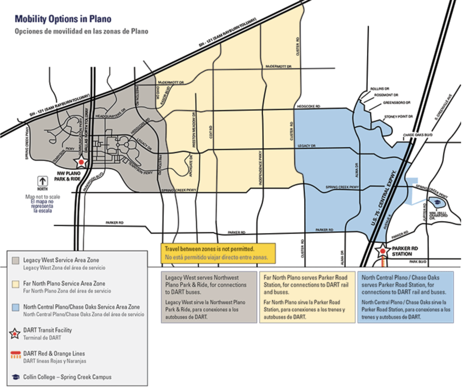
(a) GoLink in Dallas, TX (Plano region) utilizes a zone-based route structure.

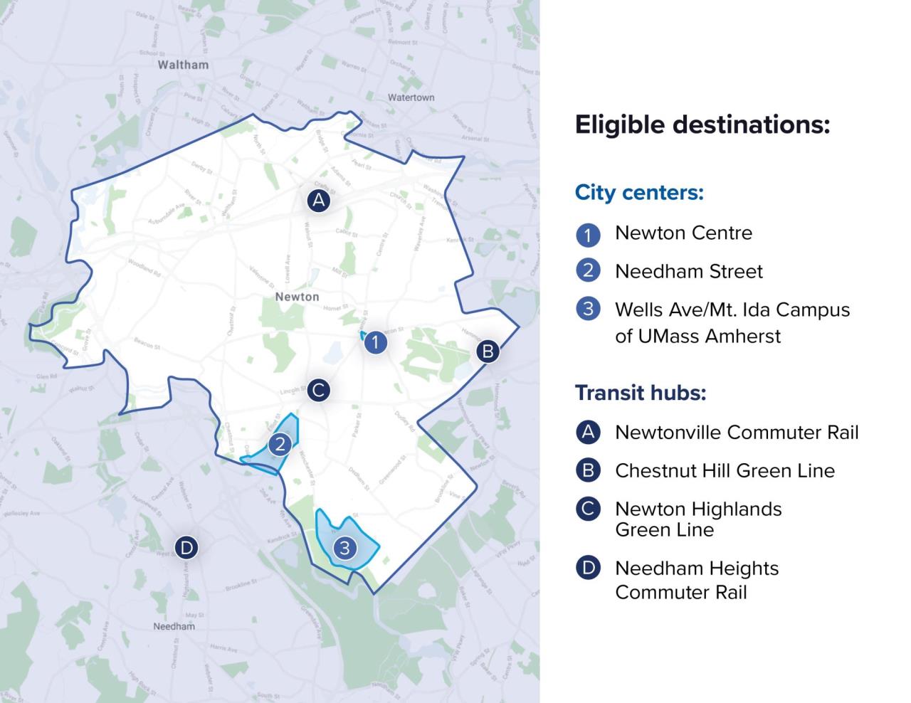
(b) The NewMo Pilot in Newton, MA utilized a hub-based route structure.

Figure 1: Route structures of recent pricing alliances. In Plano (Dallas Area Rapid Transit 2020), passengers spend up to $3 to travel anywhere within a color-blocked region. In the NewMo Pilot (City of Newton, MA 2021), passengers could travel anywhere within town limits for $2, as long as either trip endpoint was one of seven hubs. NewMo now allows passengers to travel anywhere within Newton.

Pricing alliances are characterized by the intended service populations and the relationship of the MOD operator’s system to the fixed-route transit network. Service population may be a targeted demographic, e.g. persons with limited mobility, low-income people, or senior citizens; the service population might also constitute residents of a particular geographic area, e.g. residents of a transit desert or people traveling within a given radius of a transit hub. The MOD infrastructure may complement, substitute, or extend fixed-route options. Once participating operators establish the nature of the pricing alliance, the alliance can select a joint pricing scheme. Carefully designed fares influence passenger behavior, incentivizing choices that benefit the entire system. Table 1 surveys these traits of recent pricing alliances:

• MOD operator: This can be a TNC like Uber or Lyft, or a microtransit platform like Via.

• Service population: Recent alliances have served people with limited mobility, seniors, essential workers, or simply everyone.

• Fare structure: For passengers traveling within the system, some alliances charge a flat fare and/or a variable fare based on distance travelled. Selectively applied, interpretable discount structures for jointly offered routes can encourage multimodal travel and engineer outcomes desired by the operators.

• Route structure: Alliances often require specific trip geography: point-to-point (PTP) (trips must occur within a given geographic region), zone-based (partitions a larger region into small zones and requires intra-zonal trips), and hub-based (at least one trip endpoint must be anchored at specified locations). Figure 1 illustrates zone-based and hub-based route structures.

• Integration into public transit network: The MOD portion of the network might integrate into the transit network in several ways: complementary (provides another mode option to improve service quality), substitutive (replaces existing fixed-route transit), first-/last-mile (FLM) (connects travelers to the fixed-route network), and extension (serves transit desert regions).

Table 1: Survey of recent pricing alliances. PTP: point-to-point. Flat fare: same price for every passenger. Mode: fares vary by travel mode. Distance: fares increase with distance traveled. (Dallas Area Rapid Transit 2020, Regional Transp. Commission of Southern Nevada 2021, City of Seattle, WA 2021, MBTA 2021, City of Newton, MA 2021, City of Jersey City, NJ 2021, St. Louis Metro 2021, MARTA 2021, Indianapolis Public Transp. Corporation 2021) ^∗ Not operated by a transit agency. ^∗∗ Specially marketed for senior citizens. ^∗∗∗ Available to everyone, but only in case of transit closures. ^∗∗∗∗ Transported essential workers at the beginning of the COVID-19 pandemic.

Program	City	Transit agency	MOD Op.	Service population	Fares	Routes	Integration
GoLink	Dallas, TX	DART	Via	Everyone	Mode	Zone	Complementary, FLM
RTC On-demand Pilot	Las Vegas, NV	RTC	Lyft	Paratransit	Distance	PTP	Substitutive
Via to Transit	Seattle, WA	King County Metro	Via	Everyone	Flat fare	Hub	Complementary, FLM
The RIDE Flex	Boston, MA	MBTA	Uber, Lyft	Paratransit	Flat fare	PTP	Substitutive
NewMo Pilot	Newton, MA	City of Newton∗	Via	Everyone, seniors∗∗	Flat fare	Hub	Extension, FLM
No program name	Jersey City, NJ	NJ TRANSIT	Via	Everyone	Distance	Zone	Complementary, extension
No program name	St. Louis, MO	St. Louis Metro	Lyft	Everyone	Distance	Hub	Complementary, FLM
MARTAConnect	Atlanta, GA	MARTA	Uber, Lyft	Everyone (closures)∗∗∗	Distance	PTP	Extension
IndyGo + Uber	Indianapolis, IN	IndyGo	Uber	Essential workers∗∗∗∗	Flat fare	PTP	Substitutive

1.2 Literature Review

This work sits at the intersection of literature on FLM system design and operations management, integrated multimodal transport system design, and horizontal cooperation among competing transportation operators.

FLM system design and operations: Research on demand responsive connector (DRC) systems develops analytical models to evaluate service quality and determine first-mile system parameters. In particular, such work specifies optimal zone size and headways, identifies transition points between regions best serviced by fixed-route vs. flexible services, and establishes best practices for inter-zone transfer coordination (Chandra and Quadrifoglio 2013, Kim, Levy, and Schonfeld 2019, Kim and Schonfeld 2014, Lee and Savelsbergh 2017, Li and Quadrifoglio 2010, Lu, Quadrifoglio, and Petrelli 2017, Lu, Shen, and Quadrifoglio 2014). The tactical question of how to operate a first-mile system is also well-studied. The Dial-A-Ride Problem (DARP) encompasses the vehicle routing problem faced by transit agencies, given a set of trip requests and a vehicle fleet (Ho et al. 2018, Molenbruch, Braekers, and Caris 2017). The Integrated DARP (IDARP) designs vehicle routes and schedules to meet trip requests, allowing transfers with fixed-route timetabled service (Posada, Andersson, and Hall 2017). Closely related to IDARP is the problem of matching individual carpoolers and integrating their trips with transit timetables (Stiglic et al. 2018). Finally, many studies design strategies for routing and scheduling (Wang 2019), pricing (Chen and Wang 2018), and trip request acceptance (Agussurja, Cheng, and Lau 2019) for FLM transportation systems.

Multimodal network optimization with endogenous demand: Our work is related to literature on optimal design and operation of transportation systems that acknowledges and leverages endogenous demand. Past research has modeled decision-making travelers with preferences. One-to-one and many-to-one assignment problems among travelers and suppliers have been addressed with preference-based stable matchings to prevent participants from leaving ride-sharing systems (Wang, Agatz, and Erera 2018) or transit systems (Rasulkhani and Chow 2019). Passenger decisions are also often captured by discrete choice models. Bertsimas, Ng, and Yan (2020) jointly determine frequencies and prices for multimodal transit to minimize wait times, subject to passenger mode and route choices. Cadarso et al. (2017) optimize airline scheduling, fleet assignment, and fares while capturing the effects of competing high-speed rail service, taking passengers’ mode choices into consideration. Wei, Vaze, and Jacquillat (2020) develop fixed-route transit timetables to maximize welfare, subject to competition with ride-sourcing companies, and congestion effects from passengers’ mode switching. Wang, Jacquillat, and Vaze (2022) optimize a network of vertiports for supporting urban aerial mobility, with passenger mode choices described by two alternative models, including a multinomial logit model. Banerjee et al. (2021) tackle a welfare-maximizing system design and pricing problem for centrally coordinated multimodal transport networks with price-dependent demand, and formulate it using mixed-integer convex optimization. In contrast, we tackle a multi-objective pricing alliance design problem with a practically suitable pricing scheme that enables transparent price communication to passengers, but also prevents its convexification and, in turn, heightens the computational challenge.

Horizontal Cooperation: Finally, we review cooperation models among competing operators. Literature on horizontal cooperation in logistics and airline scheduling is particularly mature (Cruijssen, Dullaert, and Fleuren 2007, Guajardo and Rönnqvist 2016, Wright, Groenevelt, and Shumsky 2010, Hu, Caldentey, and Vulcano 2013). Chun, Kleywegt, and Shapiro (2017) design a liner shipping alliance with endogenous linear demand for a homogeneous product; shipping companies first trade physical capacity on respective networks, and then compete to sell substitutable products in an overlapping market. Our work also involves joint products over a shared network subject to endogenous demand, but the allied operators offer those products together rather than exchanging capacity to compete. Algaba et al. (2019) formulate an urban transportation network flow game, using exogenous passenger and cost information to coordinate a single-fare payment among competing operators. Bian and Liu (2019a, b) design mechanisms for the first-mile problem incorporating personalized passenger requirements. Siddiq, Tang, and Zhang (2021) investigate incentive mechanisms to inspire commuters to use public transportation, modeling commuters, transit agency, ride-sharing platform, municipal government, and local private enterprises as stakeholders.

Liu and Chow (2022) investigate whether competing transit agencies can share data to improve selfish outcomes when setting frequencies, subject to user equilibrium passenger flows. Policymakers can leverage results of their Bayesian game and coalition formation model to inform decisions about establishing mandatory data-sharing amongst transit operators, but the model is not amenable to large-scale operations management. The most similar study to ours in this branch of literature is by Schlicher and Lurkin (2022), who formulate a transport choice game in which operators cooperatively price their pooled resources, subject to passengers making travel choices according to a multinomial logit model. They design a market share exchange allocation rule that ensures a stable grand coalition. Their study differs from ours in that each operator offers homogeneous products with a single price to travelers with unspecified origins and destinations, thus entirely ignoring network effects. In summary, most existing studies individually model either operator or passenger incentives when designing integrated, multimodal urban transportation systems; to our knowledge, studies incorporating both strategic operators and passengers provide only general high-level intervention recommendations and rules of thumb. Our work differs in that we provide a prescriptive and strategic design framework to build pricing alliances at scale and in full operational detail.

1.3 Contributions

We propose a prescriptive pricing alliance to enable incentive-aligned collaboration between transit agencies and established ride-sharing operators. A fare-setting model is formulated to maximize total system-wide benefits across the integrated network. Our framework helps operators navigate competing alliance objectives: (1) enhancing access to high-quality public transportation options for underserved populations, (2) lowering vehicle emissions and congestion from single-occupancy vehicle trips, and (3) maintaining the financial well-being of participating operators to ensure that the profit-oriented operators are incentivized to participate. A key technical challenge when optimizing these objectives lies in capturing interdependencies between fares and commuters’ travel choices. In response, our model integrates a discrete choice model of passengers’ route and mode decisions based on prices and non-pricing attributes like travel times.

From a technical standpoint, our fare-setting model is a large-scale, mixed-integer, non-convex optimization problem—a challenging class of problems. Our first technical contribution is to design a two-stage decomposition in which the first-stage pricing decisions parameterize second-stage fare discounts and the induced passenger behaviors. The second stage becomes a more tractable mixed-integer linear optimization problem that can be solved with commercial solvers. To solve the full model, we develop a new solution approach combining tailored coordinate descent, parsimonious second-stage evaluations, and interpolations using Special Ordered Sets of type 2 (SOS2) (Misener and Floudas 2010). We also develop acceleration techniques based on slanted coordinate traversal and search direction randomization. This solution approach—our second technical contribution—is applicable to any two-stage formulation with a low-dimensional, convex, continuous first-stage and any computationally expensive black-box second stage. This solution approach is found to significantly improve outcomes, for passengers and operators, compared to those obtained with state-of-the-art benchmarks based on Bayesian Optimization (Mockus 2012).

From a practical standpoint, we design a large-scale case study focused on the morning commute in the Greater Boston Area. We find that our model sets fares that are in realistic ranges and have interpretable connections to alliance goals. For example, an alliance with a greater focus on minimizing total VMT prefers flat rather than distance-varying fares to increase system utilization by long-distance commuters. On the other hand, alliances with a greater emphasis on increasing transit access will set discounts with greater geographic variation to make alliance routes more attractive to heterogeneous populations. The clear alignment between operator goals and passenger choices achieved by our fare structures illustrates the value of modeling endogenous demand. Moreover, analysis of our results shows that the model is appropriately responsive to equity-oriented objectives: it enables the alliance to lower fares for, and increase utilization by, low-income and long-distance commuters. Finally, when compared to non-cooperative pricing, our fares and our tailored revenue allocation mechanism together incentivize revenue-oriented MOD operators not only to participate in the alliance but also to adopt the transit operator’s priorities.

Section 2 presents the allied fare-setting model formulation, its two-stage decomposition enabling tractable solutions, as well as our revenue allocation mechanism. Section 3 describes our parsimonious SOS2-based coordinate descent approach, whose computational performance is compared against benchmarks in Section 4. We present our practical insights in Section 5 and conclude in Section 6.

2 Pricing Alliance Design Problem

We now present our design pipeline for the Pricing Alliance Design Problem (PADP). In the PADP, the alliance—i.e., the jointly acting operators—sets a fare structure that optimizes joint operator priorities over the integrated multimodal network, subject to the passengers’ endogenous route choice decisions. The individual operators must then decide whether or not to participate in the alliance they have designed based on the optimized fares and a revenue allocation mechanism.

2.1 Assumptions

Before formulating the allied fare-setting model, we specify our characterization of system-wide benefits, our model of passenger decision-making, and our assumptions about static fares.

System-wide benefits.

The alliance cooperatively set fares over an integrated network with the objective of maximizing overall benefits to society, including travelers, operators, and the rest of society (Daganzo 2012). Consistent with the motivation of this work, we assume that transit agency’s own objective is identical to that of the alliance. We characterize an operator’s benefits as its fare revenue and a passenger’s benefits as its average utility across all available travel options. High passenger utility corresponds to the availability of many high-quality travel options. Finally, there are many ways to capture the system’s impact on the rest of society, defined as everyone except the travelers and operators. Most people who take alternative travel options choose to drive personal vehicles, contributing to negative externalities, such as air pollution. Because a pricing alliance involves no change in permanent infrastructure but rather better utilization of the existing infrastructure, the key benefits of the alliance to the rest of society are likely to come from single-occupancy VMT reduction under the allied pricing regime. We ultimately compute system-wide benefits as a weighted sum of operator revenue, passenger utility, and a penalty for the outside-option VMT. The weights are determined by the alliance’s relative priorities and can be varied to evaluate trade-offs.

Passenger discrete choice model.

We model travelers as rational agents making travel decisions according to a multinomial logit (MNL) discrete choice model. In an MNL model, the choice probabilities are proportional to each option’s exponentiated utility, also known as its attractiveness (McFadden 1974). The MNL choice model allows us to embed a closed form of the passengers’ decision-making process in the alliance fare-setting model, but it also presents limitations related to the independence of irrelevant alternatives (IIA) property. Some have circumvented such inaccuracies by using the general attraction model (GAM), of which the MNL model is a special case (Gallego, Ratliff, and Shebalov 2015). The GAM formulates each choice probability as a function not only of the available options’ attractiveness, but also the shadow attractiveness of unavailable options. In practice, researchers have set the shadow attractiveness values to zero, in the absence of reliable data to estimate these parameters (Wei, Vaze, and Jacquillat 2020). Others leverage the nested MNL (Williams 1977), of which the MNL is also a special case. Lo, Yip, and Wan (2004) and Bertsimas, Ng, and Yan (2020) assume that passengers select travel mode in the first level, and then they select a route under that mode in the second level. In our work, we populate passengers’ route choice sets with the fastest route from each available travel mode (transit-only, MOD-only, or transit-MOD hybrid), including the option to drive, referred to in the literature as the outside option or the no purchase alternative. Thus, our simplified choice model framework is equivalent to a GAM with zero shadow attractiveness values, or to a mode-route nested MNL with second-level choice sets containing one route each.

Fare-setting.

The alliance sets fares over the integrated network. Some MOD operators might set time-varying fares on their independently operated network. In particular, TNCs may implement fare multipliers to manage two-sided markets between drivers and riders (Castillo, Knoepfle, and Weyl 2017). In a pricing alliance, however, the MOD operator is a contractor to the transit agency and consequently agrees to set time- and demand-homogeneous fares over allied network. This agreement facilitates transparent communication with passengers who can easily anticipate public sector prices, and it also allows the transit operator to set a budget for the alliance with higher confidence. We also assume that each operator is capable of serving all demand redistribution that occurs as a result of the newly set fares, and that capacity reallocation is therefore unnecessary to consider in the pricing alliance design process. Schlicher and Lurkin (2022) make a similar assumption: they assume a constant marginal cost due to market shares that do not change significantly. From a transit perspective, this implies that the fixed-route options (e.g., buses) have low load factors to start with, especially in and near transit deserts; on the MOD side, it implies that the operators have large driver pools driven by private market dynamics. In summary, we assume that the load difference on the integrated network when transitioning from non-cooperative to allied fare-setting will not impose a large enough change in network utilization to necessitate consideration of the associated resource allocation decisions. In the practical case study of Section 5, we validate this assumption by showing that the potential pricing alliances indeed do not pose a risk of over-saturating the integrated infrastructure.

2.2 Exact Formulation

We now provide notation for formulating our allied fare-setting model with endogenous demand. Passengers select from a set of routes, $\mathcal{R}$, serviced by a set of operators, $\mathcal{O}$, which includes a public transit operator and an MOD operator, so that $|\mathcal{O}|=2$. A route is a sequence of trip legs, each served by some operator’s infrastructure. To capture flat and distance-based fares, we define non-discounted price of route $r\in\mathcal{R}$ as:

$$\sum_{k\in\mathcal{O}_{r}}(\beta_{k}^{0}+\Delta_{rk}\cdot\beta_{k}^{\Delta})$$ (1)

where $\mathcal{O}_{r}\subseteq\mathcal{O}$ is the set of operators serving route $r$; $\Delta_{rk}$ is the distance of route $r$ covered by operator $k$; and $\beta^{0}_{k}$ and $\beta_{k}^{\Delta}$, respectively, are the base fare, and markup per unit distance traveled, for operator $k$’s sub-network. We collectively refer to the base fares and distance-based markups of all operators as the fare parameters ($\beta$), which are decision variables in our model. Fare parameters are constrained by (non-negative) upper and lower bounds ($(\beta_{\min}^{0},\beta_{\max}^{0})$, $(\beta_{\min}^{\Delta},\beta_{\max}^{\Delta})$) determined by local legislative or operational requirements.

In addition to the fare parameters, the operators jointly select a set of discounted routes. Only a subset of routes, $\mathcal{R}^{DE}\subseteq\mathcal{R}$, may be discount-eligible (DE). Rather than deciding whether or not each individual route should receive a discount, the discount-eligible routes may be grouped into discount activation categories. Routes in the same discount activation category may share common geographic components specified by the alliance. By grouping routes into categories, passengers can easily interpret which routes are discounted from a map or a simple set of rules. Example definitions for discount activation categories might include all routes anchored on a particular hub location, or all routes whose origins and destinations are contained in specified regions. Let $\mathcal{R}_{a}\subset\mathcal{R}$ be the set of routes corresponding to discount activation category $a\in\mathcal{A}.$ The sets $\mathcal{R}_{a}$ partition $\mathcal{R}^{DE},$ i.e., $\cup_{a\in\mathcal{A}}\mathcal{R}_{a}=\mathcal{R}^{DE}$ and $\mathcal{R}_{a}\cap\mathcal{R}_{b}=\emptyset$ for $a\neq b\in\mathcal{A}$. Let $x_{a}\in\{0,1\}$ denote the decision variable that activates discounts on all routes in $\mathcal{R}_{a}$. This assumption is not restrictive; absence of activation categories can be handled easily by putting each route in its own category: $|\mathcal{R}_{a}|=1,\forall a\in\mathcal{A}$. We note that the relaxation of this assumption might result in discount rules that are difficult to communicate to passengers in large-scale systems.

$\Lambda$ is the discount multiplier for the routes selected to receive a discount, with an allowable range of $[\Lambda^{min},\Lambda^{max}]:0\leq\Lambda^{min}\leq\Lambda^{max}\leq 1.$ The customer-facing price, $p_{r}$, of route $r\in\mathcal{R}$, is given as:

$$p_{r}=\begin{cases}(1-\Lambda\cdot x_{a})\cdot\left(\sum_{k\in\mathcal{O}_{r}}(\beta_{k}^{0}+\Delta_{rk}\cdot\beta_{k}^{\Delta})\right)&\text{if }\>r\in\mathcal{R}_{a},a\in\mathcal{A}\\ \sum_{k\in\mathcal{O}_{r}}(\beta_{k}^{0}+\Delta_{rk}\cdot\beta_{k}^{\Delta})&\text{if }\>r\in\mathcal{R}\setminus\mathcal{R}^{DE}\end{cases}$$ (2)

We consider a set $\mathcal{N}$ of passenger types. Each passenger type $i\in\mathcal{N}$ is identified by a unique combination of origin, destination, and preference profile as described by their route choice utility coefficients. $\mathcal{R}_{i}$ is the set of routes available to passengers of type $i\in\mathcal{N}$. Some passengers are more averse to expensive travel options, whereas others are more sensitive to travel time, constituting different preference profiles. There are $N_{i}$ passengers of type $i\in\mathcal{N}$. We denote the utility to a passenger of type $i\in\mathcal{N}$ of route $r\in\mathcal{R}_{i}$ as $u_{ir}+\alpha_{i}\cdot p_{r}$, where ${u}_{ir}$ is the utility from non-monetary route attributes and $\alpha_{i}\leq 0$ is the utility per unit price. The market share $s_{ir}$ of route $r\in\mathcal{R}_{i}$ for passenger type $i\in\mathcal{N}$ is computed according to MNL as:

$$s_{ir}=\frac{\exp(u_{ir}+\alpha_{i}\cdot p_{r})}{\exp(u_{i0})+\sum_{s\in\mathcal{R}_{i}}\exp(u_{is}+\alpha_{i}\cdot p_{s})},$$ (3)

where the outside option—not in set $\mathcal{R}=\bigcup_{i\in\mathcal{N}}\mathcal{R}_{i}$—has a utility $u_{i0}$ and a market share computed as:

$$s_{i0}=\frac{\exp(u_{i0})}{\exp(u_{i0})+\sum_{s\in\mathcal{R}_{i}}\exp(u_{is}+\alpha_{i}\cdot p_{s})}.$$ (4)

Finally, the operators’ relative priorities over the system-wide performance metrics are captured by non-negative objective function weights: $\mu^{PAX},\mu^{REV},\mu^{VMT}$, respectively, corresponding to passenger benefits, operator benefits, and the benefits from negative externality reduction. Table 2 summarizes all notation. Model PADP-FS (5)-(13) provides the exact formulation for the PADP fare-setting model. It jointly sets fares and discounts to maximize system-wide benefits across the integrated network (objective function (5)). Discounts are applied on selected routes (Constraints (6) and (7)) and utility-maximizing passengers make route selections according to an MNL (Constraints (8) and (9)). Fare parameters and the discount multipliers obey bounds (Constraints (10)-(12)). Discount activation decisions are binary (Constraints (13)).

Table 2: Notation.

Component	Type	Description
$\mathcal{A}$	Set	Discount activation categories
$\mathcal{N}$	Set	Passenger types
$\mathcal{O}$	Set	Operators
$\mathcal{R}$	Set	Intrasystem routes, not including the outside option
$\mathcal{O}_{r}$	Set	Operators who help service route $r\in\mathcal{R}$
$\mathcal{R}_{i}$	Set	Route options available to passengers of type $i\in\mathcal{N}$
$\mathcal{R}_{a}$	Set	Routes in discount activation category $a\in\mathcal{A}$
$\mathcal{R}^{DE}$	Set	Discount-eligible routes, i.e., $\bigcup_{a\in\mathcal{A}}\mathcal{R}_{a}$
$N_{i}$	Param.	Number of passengers of type $i\in\mathcal{N}$
$\Delta_{i0}$	Param.	Driving distance for a passenger of type $i\in\mathcal{N}$
$\Delta_{rk}$	Param	Distance the passenger travels with operator $k\in\mathcal{O}$ on route $r\in\mathcal{R}$
$u_{ir}$	Param.	Non-monetary utility accrued by a passenger of type $i\in\mathcal{N}$ on route $r\in\mathcal{R}_{i}$
$u_{i0}$	Param.	Utility accrued by a passenger of type $i\in\mathcal{N}$ by driving
$\alpha_{i}$	Param.	Utility per unit price to a passenger of type $i\in\mathcal{N}$
$\beta^{0}_{min},\beta^{0}_{max}$	Param.	Minimum and maximum allowable base fares
$\beta^{\Delta}_{min},\beta^{\Delta}_{max}$	Param.	Minimum and maximum allowable distance-based markups
$\Lambda^{min},\Lambda^{max}$	Param.	Minimum and maximum allowable values of discount multipliers
$\mu^{PAX},\mu^{REV},\mu^{VMT}$	Param.	Relative priority weights of system-wide performance metrics
$x_{a}$	Var.	Binary. Whether to activate discount option $a\in\mathcal{A}$
$\beta_{k}^{0},\beta_{k}^{\Delta}$	Var.	Continuous. Base fare and markup of operator $k\in\mathcal{O}$
$p_{r}$	Var.	Continuous. Customer-facing price of route $r\in\mathcal{R}$
$\Lambda$	Var.	Continuous. Discount multiplier applied to routes with activated discounts
$s_{ir}$	Var.	Continuous. Proportion of passengers of type $i\in\mathcal{N}$ who choose route $r\in\mathcal{R}_{i}$
$s_{i0}$	Var.	Continuous. Proportion of passengers of type $i\in\mathcal{N}$ who choose the outside option

$$(\text{PADP-FS})\qquad\max\quad\sum_{i\in\mathcal{N}}N_{i}\cdot\Big{[}\mu^{PAX}\cdot\big{(}u_{i0}+\sum_{r\in\mathcal{R}_{i}}(u_{ir}+\alpha_{i}\cdot p_{r})\big{)}+\mu^{REV}\cdot\sum_{r\in\mathcal{R}_{i}}p_{r}\cdot s_{ir}-\mu^{VMT}\cdot(\Delta_{i0}\cdot s_{i0})\Big{]}$$ (5)

s.t. $$p_{r}=\sum_{k\in\mathcal{O}_{r}}(\beta_{k}^{0}+\Delta_{rk}\cdot\beta_{k}^{\Delta}) r\in\mathcal{R}\setminus\mathcal{R}^{DE}$$ (6)

$$p_{r}=(1-\Lambda\cdot x_{a})\cdot\left(\sum_{k\in\mathcal{O}_{r}}(\beta_{k}^{0}+\Delta_{rk}\cdot\beta_{k}^{\Delta})\right) a\in\mathcal{A},r\in\mathcal{R}_{a}$$ (7)

$$s_{ir}=\frac{\exp(u_{ir}+\alpha_{i}\cdot p_{r})}{\exp(u_{i0})+\sum_{s\in\mathcal{R}_{i}}\exp(u_{is}+\alpha_{i}\cdot p_{s})} i\in\mathcal{N},r\in\mathcal{R}_{i}$$ (8)

$$s_{i0}=\frac{\exp(u_{i0})}{\exp(u_{i0})+\sum_{s\in\mathcal{R}_{i}}\exp(u_{is}+\alpha_{i}\cdot p_{s})} i\in\mathcal{N}$$ (9)

$$\beta_{min}^{0}\leq\beta_{k}^{0}\leq\beta_{max}^{0} k\in\mathcal{O}$$ (10)

$$\beta_{min}^{\Delta}\leq\beta_{k}^{\Delta}\leq\beta_{max}^{\Delta} k\in\mathcal{O}$$ (11)

$$\Lambda^{min}\leq\Lambda\leq\Lambda^{max}$$ (12)

$$x_{a}\in\{0,1\} a\in\mathcal{A}$$ (13)

2.3 Two-stage Decomposition

The PADP-FS model is a non-convex mixed-integer nonlinear optimization problem (MINLOP). There are no commercial solvers that accommodate non-convex MINLOPs, and no open-source solvers accept non-convex MINLOPs at practically large scale. Therefore, we propose a different solution approach. We decompose the formulation to tractably obtain high-quality solutions for practically sized problems (tens of thousands of variables and hundreds of thousands of constraints in our case study). By letting first-stage pricing decisions parameterize second-stage discount activations and induced passenger behaviors, the second stage can be formulated as a more tractable mixed integer linear optimization problem (MILOP).

Let $\mathcal{B}:=[\beta_{min}^{0},\beta_{max}^{0}]^{2}\times[\beta_{min}^{\Delta},\beta_{max}^{\Delta}]^{2}$ and $\mathcal{L}:=[\Lambda^{min},\Lambda^{max}]$ respectively be the sets of allowable fare parameters and discount multipliers. We parameterize the second-stage problem by $(\bm{\widehat{\beta}},\widehat{\Lambda})\in\mathcal{B}\times\mathcal{L}$ and define $\mathcal{S}(\widehat{\bm{\beta}},\widehat{\Lambda})$ as the feasible region parameterized by $(\bm{\widehat{\beta}},\widehat{\Lambda})$. We utilize the sales-based linear optimization formulation by Gallego, Ratliff, and Shebalov (2015) to reformulate the choice model constraints. The premise of the reformulation rests on proportionality constraints. Let $\gamma_{ir}=\exp(u_{i0})/\exp(u_{ir}+\alpha_{i}\cdot p_{r})$ be the ratio of the attractiveness values of the outside option and route $r\in\mathcal{R}_{i}$. Since the fare parameters are determined in the first stage, $\gamma_{ir}$ is a constant in the second stage formulation for the non-discount-eligible routes. Then constraints (8) and (9) are reformulated as follows:

$$s_{i0}=\gamma_{ir}\cdot s_{ir} i\in\mathcal{N},r\in\mathcal{R}_{i}$$ (14)

$$s_{i0}+\sum_{r\in\mathcal{R}_{i}}s_{ir}=1 i\in\mathcal{N}$$ (15)

$$s_{i0}\geq 0 i\in\mathcal{N}$$ (16)

$$s_{ir}\geq 0 i\in\mathcal{N},r\in\mathcal{R}_{i}$$ (17)

Equation (14) ensures that the market share of each route is proportional to its attractiveness. Constraints (15), (16), and (17) ensure that the market shares are non-negative and sum to 1. Note that Equation (14) still includes bilinearities for discount-eligible routes $r\in\mathcal{R}_{i}\cap\mathcal{R}^{DE}$. For a type $i$ passenger, $\gamma_{ir}$ is either equal to the discounted price ($\gamma_{ir}=\gamma_{ir}(\widehat{\bm{\beta}},\widehat{\Lambda})$) or full price ($\gamma_{ir}=\gamma_{ir}(\widehat{\bm{\beta}},0)$), depending on whether the model selects the discount for route $r$. Let $\mathcal{N}_{a}\subset\mathcal{N}$ be the set of passenger types with at least one route option corresponding to discount activation category $a\in\mathcal{A}$. We linearize constraint (14) as (18) using big-$M$ constraints, letting $M_{ir}^{s}=\gamma_{ir}(\widehat{\bm{\beta}},0)\geq 0$.

$$\begin{cases}s_{i0}\leq\gamma_{ir}(\bm{\widehat{\beta}},0)\cdot s_{ir}\\ s_{i0}\geq\gamma_{ir}(\bm{\widehat{\beta}},0)\cdot s_{ir}-M_{ir}^{s}\cdot x_{a}\\ s_{i0}\leq\gamma_{ir}(\bm{\widehat{\beta}},\widehat{\Lambda})\cdot s_{ir}+M_{ir}^{s}\cdot(1-x_{a})\\ s_{i0}\geq\gamma_{ir}(\bm{\widehat{\beta}},\widehat{\Lambda})\cdot s_{ir}\end{cases}\qquad a\in\mathcal{A},i\in\mathcal{N}_{a},r\in\mathcal{R}_{i}\cap\mathcal{R}_{a}$$ (18)

We similarly handle the bilinearities presented by the revenue terms in the objective function. We define a new decision variable $w_{ir}=p_{r}\cdot s_{ir}$ for passenger types $i\in\mathcal{N}$ with discount-eligible routes $r\in\mathcal{R}_{i}\cap\mathcal{R}^{DE}$. The linearized constraints (19) set the value of $w_{ir}$ with $M_{ir}^{w}=\widehat{\Lambda}\cdot\left(\sum_{k\in\mathcal{O}_{r}}(\widehat{\beta}_{k}^{0}+\Delta_{rk}\cdot\widehat{\beta}_{k}^{\Delta})\right)\geq 0$.

$$\begin{cases}w_{ir}\leq\left(\sum_{k\in\mathcal{O}_{r}}(\widehat{\beta}_{k}^{0}+\Delta_{rk}\cdot\widehat{\beta}_{k}^{\Delta})\right)\cdot s_{ir}\\ w_{ir}\geq\left(\sum_{k\in\mathcal{O}_{r}}(\widehat{\beta}_{k}^{0}+\Delta_{rk}\cdot\widehat{\beta}_{k}^{\Delta})\right)\cdot s_{ir}-M_{ir}^{w}\cdot x_{a}\\ w_{ir}\leq(1-\widehat{\Lambda})\cdot\left(\sum_{k\in\mathcal{O}_{r}}(\widehat{\beta}_{k}^{0}+\Delta_{rk}\cdot\widehat{\beta}_{k}^{\Delta})\right)\cdot s_{ir}+M_{ir}^{w}\cdot(1-x_{a})\\ w_{ir}\geq(1-\widehat{\Lambda})\cdot\left(\sum_{k\in\mathcal{O}_{r}}(\widehat{\beta}_{k}^{0}+\Delta_{rk}\cdot\widehat{\beta}_{k}^{\Delta})\right)\cdot s_{ir}\end{cases}\qquad a\in\mathcal{A},i\in\mathcal{N}_{a},r\in\mathcal{R}_{i}\cap\mathcal{R}_{a}$$ (19)

Table 3 summarizes the additional and modified notation for the second-stage model.

Table 3: Additional and modified notation for second-stage model of the decomposition framework.

Component	Type	Description
$\mathcal{B}$	Set	Allowable fare parameter values
$\mathcal{L}$	Set	Allowable percent discount values
$\mathcal{N}_{a}$	Set	Passenger types with access to at least one discount-eligible route in
		discount activation category $a\in\mathcal{A}$, i.e. $\mathcal{R}_{i}\cap\mathcal{R}_{a}\neq\emptyset$
$\gamma_{ir}(\bm{\beta},\Lambda)$	Parameter	Ratio of outside option attractiveness to attractiveness of route $r\in\mathcal{R}_{i}$
		with price parameters $\bm{\beta}$ and discount $\Lambda$ for passenger type $i\in\mathcal{N}$
$M_{ir}^{w},M_{ir}^{s}$	Parameter	Big-$M$ parameters for each $i\in\mathcal{N},r\in\mathcal{R}_{i}$
$w_{ir}$	Variable	Continuous. Equivalent to $p_{r}\cdot s_{ir}$ for discount-eligible routes $r\in\mathcal{R}_{i}\cap\mathcal{R}^{DE}$

In response to fare parameters set in the first stage, the second-stage problem activates discounts that optimize system-wide performance metrics, subject to induced passenger decisions. The optimal value of the second-stage problem is denoted by $W$ in equation (20).

$$W(\bm{\widehat{\beta}},\widehat{\Lambda}):=\max_{(\bm{x},\bm{s},\bm{w},\bm{p})\in\mathcal{S}(\bm{\widehat{\beta}},\widehat{\Lambda})}\sum_{i\in\mathcal{N}}N_{i}\cdot\Big{[}\mu^{PAX}\cdot\big{(}u_{i0}+\sum_{r\in\mathcal{R}_{i}}(u_{ir}+\alpha_{i}\cdot p_{r})\big{)}+\mu^{REV}\cdot\sum_{r\in\mathcal{R}_{i}}w_{ir}-\mu^{VMT}\cdot(\Delta_{i0}\cdot s_{i0})\Big{]},$$ (20)

where $\mathcal{S}(\bm{\widehat{\beta}},\widehat{\Lambda})$ is given as follows:

$$\mathcal{S}(\bm{\widehat{\beta}},\widehat{\Lambda})\,\equiv\Big{\{}(\bm{x},\bm{s},\bm{w},\bm{p})\in\{0,1\}^{|\mathcal{A}|}\times\mathbb{R}_{+}^{\sum_{i\in\mathcal{N}}(|\mathcal{R}_{i}|+1)}\times\mathbb{R}^{\sum_{i\in\mathcal{N}}|\mathcal{R}_{i}\cap\mathcal{R}^{DE}|}\times\mathbb{R}^{|\mathcal{R}|}\,:\,\qquad\qquad\qquad\qquad\qquad$$

Constraints (18) - (19)

$$s_{i0}+\sum_{r\in\mathcal{R}_{i}}s_{ir}=1 i\in\mathcal{N}$$ (21)

$$s_{i0}=\gamma_{ir}(\bm{\widehat{\beta}},0)\cdot s_{ir} i\in\mathcal{N},r\in\mathcal{R}_{i}\setminus\mathcal{R}^{DE}$$ (22)

$$w_{ir}=\left(\sum_{k\in\mathcal{O}_{r}}(\widehat{\beta}_{k}^{0}+\Delta_{rk}\cdot\widehat{\beta}_{k}^{\Delta})\right)\cdot s_{ir} i\in\mathcal{N},r\in\mathcal{R}_{i}\setminus\mathcal{R}^{DE}$$ (23)

$$p_{r}=\sum_{k\in\mathcal{O}_{r}}(\widehat{\beta}_{k}^{0}+\Delta_{rk}\cdot\widehat{\beta}_{k}^{\Delta}) r\in\mathcal{R}\setminus\mathcal{R}^{DE}$$ (24)

$$p_{r}=(1-\widehat{\Lambda}\cdot x_{a})\cdot\left(\sum_{k\in\mathcal{O}_{r}}(\widehat{\beta}_{k}^{0}+\Delta_{rk}\cdot\widehat{\beta}_{k}^{\Delta})\right) a\in\mathcal{A},r\in\mathcal{R}_{a} \Big{\}}$$ (25)

Then we define the PADP-FS2SD model, the two-stage decomposition of the PADP-FS model.

$$(\text{PADP-FS2SD})\qquad\max\quad W(\bm{\beta},\Lambda)$$ (26)

s.t. $$\bm{\beta}\in\mathcal{B}$$ (27)

$$\Lambda\in\mathcal{L}$$ (28)

Lemma 2.1

Formulations PADP-FS and PADP-FS2SD are equivalent.

The proof of Lemma 2.1 is in Appendix 7.

2.4 Revenue Allocation Mechanism

When considering a pricing alliance, an operator assesses whether the cooperative regime would improve its prioritized system-wide metrics over the non-cooperative regime. A non-cooperative fare-setting game and a solution approach for it are presented in Appendix 8. The MOD operator is solely revenue-maximizing, while the transit agency maximizes a linear combination of multiple system-wide metrics. By entering a pricing alliance, the transit agency (denoted as TR) is guaranteed to fare no worse than that under the non-cooperative regime. However, it remains to ensure that the revenue-maximizing MOD operator will not lose revenue by cooperating with the transit agency, which would ensure the MOD operator’s participation.

We now design a revenue allocation mechanism that guarantees the MOD operator’s alliance participation. Let $\bm{\beta}^{nc}$ and $(\bm{\beta}^{a},\Lambda^{a})$ respectively denote the non-cooperative equilibrium fare parameters and allied optimal fare parameters. Let $f_{k}(\bm{\beta}^{nc})$ denote the revenue of operator $k\in\mathcal{O}$ in the non-cooperative regime, and $f(\bm{\beta}^{a},\Lambda^{a})$ denote the combined revenue of both operators in the alliance.

Lemma 2.2

Let $\delta=f(\bm{\beta}^{a},\Lambda^{a})-\sum_{k\in\mathcal{O}}f_{k}(\bm{\beta}^{nc})$ be the surplus allied revenue compared to the total non-cooperative revenue. Define $\Phi_{k}:\mathbb{R}^{2}_{+}\times\mathbb{R}_{+}\to\mathbb{R}_{+}$ to be the revenue allocation to operator $k\in\mathcal{O}:=\{TR,MOD\}$:

$$\Phi_{TR}((f_{k}(\bm{\beta}^{nc}))_{k\in\mathcal{O}},f(\bm{\beta}^{a},\Lambda^{a})) =\begin{cases}f_{TR}(\bm{\beta}^{nc})+\frac{\delta}{2}\cdot&\text{if }\delta\geq 0,\\ f(\bm{\beta}^{a},\Lambda^{a})-f_{MOD}(\bm{\beta}^{nc})&\text{otherwise.}\end{cases}$$ (29)

$$\Phi_{MOD}((f_{k}(\bm{\beta}^{nc}))_{k\in\mathcal{O}},f(\bm{\beta}^{a},\Lambda^{a})) =f_{MOD}(\bm{\beta}^{nc})+\big{(}\tfrac{\delta}{2}\big{)}^{+}$$ (30)

1. The MOD operator will enter the pricing alliance with payment rule $\Phi$.

2. When $\delta\geq 0$, the mechanism satisfies Pareto efficiency, symmetry, the core property, scale invariance, and independence of irrelevant alternatives.

The proof of Lemma 2.2 is in Appendix 9. Because the alliance’s priorities may also include benefits to passengers and/or benefits to the rest of the society in the form of reduced VMT, the alliance may earn less revenue than the operators’ combined revenue in the non-cooperative regime. Despite this, the transit operator can choose to guarantee that, by cooperating, the revenue-oriented MOD operator earns at least as much as it would have earned otherwise. We assume that the MOD operator will participate in the alliance if its non-cooperative and allied revenues are equal. In the event that the alliance accrues strictly more revenue than that in the non-cooperative regime, the operators split the surplus evenly.

3 Solution Approach

3.1 Motivation

Section 2.3 presented a two-stage decomposition of the allied fare-setting formulation, with the second stage characterized as a mixed-integer linear optimization problem and the first stage as a low-dimensional decision problem over a convex space. Without an analytic closed-form of $W$, the function’s gradients are inaccessible, eliminating the possibility of using any gradient-based approaches. Bayesian Optimization is applicable and has been leveraged in recent urban transportation studies focusing on MOD systems (Liu et al. 2019), but it does not provide clear convergence criteria. PADP-2SD is also not amenable to Benders decomposition due to the nonlinear interdependencies between first- and second-stage decisions. Our problem’s incompatibility with the simpler centralized welfare-maximization structure of the problem tackled by Banerjee et al. (2021) implies that their convexification strategy cannot be applied either.

Our solution strategy approximates gradient descent for solving the first-stage problem. Because the first-stage feasible space is low-dimensional and convex, we begin with a coordinate descent framework, which takes turns fixing all fare parameters except one and greedily optimizing along the free dimension. Even one-dimensional search is difficult because the search space is a continuous spectrum of optimal MILOP solutions. While a solution of the second-stage problem is fast enough to be a useful tool (see Section 4: needing at most 5 seconds on average), it is also slow enough to warrant a judicious selection of first-stage valuation points. Thus, our tailored coordinate descent approach scans each search direction by solving a model that approximates the best solution along that search direction. After evaluating a few points along the free search direction with the second-stage MILOP, an auxiliary model interpolates intermediate solutions along that search direction with Special Ordered Sets of type 2 (SOS2) (Misener and Floudas 2010). The process terminates when no improvements are found along any coordinate direction. We define this as the basic SOS2 Coordinate Descent (SOS2-CD) approach in Section 3.2.

To further improve final solution quality given a computational budget, we develop three acceleration strategies that build upon SOS2-CD. First, rather than using an arbitrary search direction sequence, we introduce more opportunities to escape local optima by randomizing search direction order. Second, we exploit the fact that the SOS2 approximation model is valid along any search direction through the first-stage problem’s search space, and not just those parallel to coordinate axes. Natural search direction candidates are those where each operator’s base fare and markup are jointly varied while holding all other parameters constant. By considering SOS2 coordinate descent over such slanted directions, we unlock directions navigating trade-offs between high base fares and low markups vs. low base fares and high markups, which would be unavailable with single-coordinate search directions. Finally, we show how to mitigate the SOS2-CD’s sensitivity to random initializations by leveraging warm-start solutions. 3.3 describes the final algorithm, including acceleration strategies, initialization procedures, and the incorporation of time limits. Computational results in Section 4 demonstrate the effectiveness of SOS2-CD and all acceleration strategies.

3.2 SOS2 Coordinate Descent

Let $\mathcal{Y}:=\mathcal{B}\times\mathcal{L}$ denote the search space over which to optimize $W$, and $\bm{y}:=(\bm{\beta},\bm{\lambda})\in\mathcal{Y}$ denote a solution. Let $\mathcal{Y}_{i}(\mathbf{y})=\{z\in\mathbb{R}\,:\,(y_{1},\cdots,y_{i-1},z,y_{i+1},\cdots,y_{n})\in\mathcal{Y}\}$ be the subset of the feasible space with all dimensions other than the $i^{th}$ fixed to those of solution $\mathbf{y}\in\mathcal{Y}$. We define $\mathcal{S}(\bm{y})$ and $\mathcal{S}^{*}(\bm{y})\subseteq\mathcal{S}(\bm{y})$, respectively, to be the set of feasible and optimal second-stage decisions given fare parameters $\bm{y}:=(\bm{\beta},\Lambda)\in\mathcal{Y}$:

$$\mathcal{S}^{*}(\bm{y}):=\arg\max_{(\bm{x},\bm{s},\bm{w},\bm{p})\in\mathcal{S}(\bm{y})}\,\sum_{i\in\mathcal{N}}N_{i}\cdot\Big{[}\mu^{PAX}\cdot\big{(}u_{i0}+\sum_{r\in\mathcal{R}_{i}}(u_{ir}+\alpha_{i}\cdot p_{r})\big{)}+\mu^{REV}\cdot\sum_{r\in\mathcal{R}_{i}}w_{ir}-\mu^{VMT}\cdot(\Delta_{i0}\cdot s_{i0})\Big{]}.$$

Basic Coordinate Descent.

Coordinate descent is a greedy method that successively optimizes a multivariate function along coordinate axes. Starting from an initial point, it cyclically optimizes along every coordinate direction holding all other dimensions fixed. Algorithm 1 presents basic coordinate descent to solve the PADP. Optimizing even a single dimension of $W$ is hard, because it entails navigating a continuous spectrum of optimal solutions to MILOPs, which does not have closed analytic form. Therefore, we will propose a rigorous method for tractably modifying Step 7 of Algorithm 1 using SOS2 interpolation.

Algorithm 1 Coordinate Descent for maximization of $W$

1:arg $\bm{y}^{0}:$ Initial solution in $\mathcal{Y}$

2:procedure Coordinate Descent($\mathbf{y}^{0}$)

3:     $objPrev\leftarrow-\infty$; $objCur\leftarrow W(\mathbf{y}^{0})$; $k\leftarrow 0$; $n\leftarrow\dim(\bm{y}^{0})$

4:     while $objCur-objPrev>\epsilon$ do

5:         $k\leftarrow k+1;objPrev\leftarrow objCur;\mathbf{y}^{k}\leftarrow\mathbf{y}^{k-1}$

6:         for  $i\in\{1,\dots,n\}$  do

7:              $y_{i}^{k}=\arg\max_{{z}\in\mathcal{Y}_{i}(\mathbf{y}^{k})}W(y^{k}_{1},\cdots,y^{k}_{i-1},z,y^{k}_{i+1},\cdots,y^{k}_{n})$          

8:         $objCur\leftarrow W(\mathbf{y}^{k})$      

9:     return $\mathbf{y}^{k}$

SOS2 Interpolation.

Our SOS2 interpolation procedure performs approximate local search along a specified direction to produce the next candidate solution. First, we solve $D$ second-stage models at evenly spaced points along the search direction, obtaining a sequence of fare parameter values acting as anchors for the SOS2 interpolation. We denote the anchors by $\bm{y}^{d}:=(\bm{\beta}^{d},\Lambda^{d})$ and their corresponding solutions by $(\bm{x}^{d},\bm{s}^{d},\bm{w}^{d},\bm{p}^{d})\in\mathcal{S}^{*}(\bm{y}^{d}),\forall d\in\{1,\dots,D\}$. Let $\Omega=\{\bm{y}^{d}\,:\,d\in\{1,\dots,D\}\}$ be the ordered set of anchors. Larger $D$ values interpolate more accurately, but the solution is also more computationally expensive.

Figure 2 visualizes the selection of the next candidate solution using SOS2 variables. $W$ is exactly evaluated at every anchor and approximated between the anchors using the interpolated anchor solutions. The next candidate solution is selected where the approximation of $W$ is maximized. Rather than directly interpolating $W$, or $\bm{w}_{ir}$ variables linearizing $p_{r}s_{ir}$ terms, we interpolate the price and market share variables, $\bm{p}$ and $\bm{s}$. Otherwise, the interpolated values of $W$ will be convex combinations of anchor valuations (straight line segments connecting consecutive anchors in Figure 2), eliminating any chance of selecting fare parameters between anchors. Moreover, since the objective function’s nonlinearities are quadratic in nature due to the multiplicative revenue terms, we capture them with this SOS2 approximation.

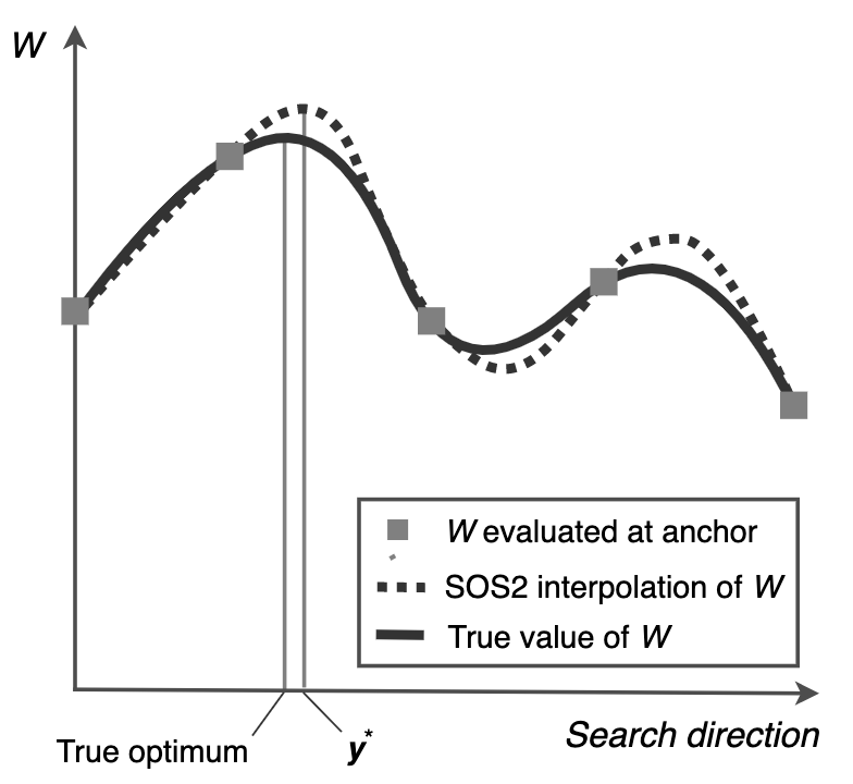
Figure 2: SOS2 interpolation of $W$ value and the selection of next candidate first-stage solution $\bm{y}^{*}$.

For a given number of anchor points D, the SOS2 model (Misener and Floudas 2010) is algebraically specified as $SOS2(D)\equiv\Big{\{}\,(\bm{\lambda},\bm{z})\in\mathbb{R}_{+}^{D}\times\{0,1\}^{D-1}\,:\,\sum_{d=1}^{D}\lambda_{d}=1,\sum_{d=1}^{D-1}z_{d}=1,\lambda_{1}\leq z_{1},\lambda_{d}\leq z_{d-1}+z_{d}\>\forall d\in\{2,\dots,D\},\lambda_{D}\leq z_{D-1}\Big{\}}$. Here, the $\bm{\lambda}$ variables are the convex combination weights for outputs at fare parameters $(\bm{\beta}^{d},\Lambda^{d})$, and each binary $z_{d}$ variable indicates whether to select the segment between anchors $d$ and $d+1$. Now we use the SOS2 variables to approximate $W$ along a given coordinate axis. Expression (31) presents the set of fare parameters, $SOS2^{*}(\Omega)$, that optimize approximated $W$ given the ordered anchor set $\Omega$. Expression (32) denotes optimal solutions at all anchors. The optimal SOS2 variables are selected to maximize the approximated $W$ function in Constraint (33). Finally, the approximately optimal fares are interpolated in equation (34). The approximated objective function is quadratic, making (33) a mixed-integer quadratic optimization problem. Fortunately, it can be solved almost instantly to global optimality with commercial solvers, because $D$ is small by design.

$$SOS2^{*} (\Omega):=$$ (31)

$$\Bigg{\{}\bm{y}\,\,:\,\, (\bm{x}^{d},\bm{s}^{d},\bm{w}^{d},\bm{p}^{d})\in\mathcal{S}^{*}(\bm{y}^{d}),\quad\forall\bm{y}^{d}\in\Omega$$ (32)

$$(\bm{\lambda}^{*},\bm{z}^{*})\in\argmax_{(\bm{\lambda},\bm{z})\in SOS2(D)}\quad\sum_{i\in\mathcal{N}}N_{i}\cdot\Big{(}\mu^{PAX}\cdot\big{(}u_{i0}+\sum_{r\in\mathcal{R}_{i}}(u_{ir}+\alpha_{i}\cdot\sum_{d\in\mathcal{D}}p_{r}^{d}\cdot\lambda_{d})\big{)}+$$

$$\qquad\qquad\mu^{REV}\cdot\sum_{r\in\mathcal{R}_{i}}\Big{(}\sum_{d\in\mathcal{D}}(p_{r}^{d}\cdot\lambda_{d})\cdot\sum_{d\in\mathcal{D}}(s_{ir}^{d}\cdot\lambda_{d})\Big{)}-\mu^{VMT}\cdot\Delta_{i0}\cdot\sum_{d\in\mathcal{D}}(s_{i0}^{d}\cdot\lambda_{d})\Big{)}$$ (33)

$$\bm{y}=\sum_{\bm{y}^{d}\in\Omega}\lambda_{d}^{*}\bm{y}^{d} \Bigg{\}}$$ (34)

Summary of SOS2 Coordinate Descent.

We present SOS2-CD in Algorithm 2, which replaces the one-dimensional optimization in Step 7 of Algorithm 1 with the SOS2-based approximation. The subroutine Search Directions provides a comprehensive ordered list of search directions that can potentially be multidimensional and/or randomized (options further discussed in the next subsection); the default is to cycle through coordinate axes, i.e. to return $searchDirections=\{1,\dots,\dim(\bm{y}^{0})\}$ when $random$ and $multidim$ are both set to $false$. The subroutine Generate Anchors returns evenly spaced SOS2 anchors along the specified search direction. The current solution is included in the anchor set to ensure that the new solution is at least as good as the previous. Appendix 10 presents subroutines Search Directions and Generate Anchors in full detail. After generating the anchors in Step 7, Step 8 computes an optimal solution for each anchor, uses these anchor solutions for interpolation, and picks the solution that maximizes approximated $W$ over the given search direction. Step 9 computes true value of $W$ at the new candidate solution and updates the current solution if necessary. The algorithm iterates until convergence.

Algorithm 2 SOS2 Coordinate Descent for maximization of $W$

1:args $\bm{y}^{0}:$ Initial solution in $\mathcal{Y}$; $D$: Number of SOS2 anchors; $random$: Boolean, whether to randomize search directions; $multidim$: Boolean, whether to use multidimensional slanted search directions

2:procedure SOS2 Coordinate Descent($\bm{y}^{0},D,random,multidim$)

3:     $objPrev\leftarrow-\infty$; $objCur\leftarrow W(\mathbf{y}^{0})$; $k\leftarrow 0$

4:     while $objCur-objPrev>\epsilon$ do

5:         $k\leftarrow k+1;objPrev\leftarrow objCur;\mathbf{y}^{k}\leftarrow\mathbf{y}^{k-1}$

6:         for  $i\in$ Search Directions ($random$, $multidim$)  do

7:              $\Omega\leftarrow$ Generate Anchors$(\bm{y}^{k},i,D)$

8:              Interpolate an optimal solution: draw some $\bm{y}^{*}$ from $SOS2^{*}(\Omega)$

9:              $\bm{y}^{k}\leftarrow\bm{y}^{*}$ if $W(\bm{y}^{*})>objCur$ else $\bm{y}^{k}$          

10:         $objCur\leftarrow W(\mathbf{y}^{k})$      

11:     return $\mathbf{y}^{k}$

3.3 Final Algorithm

We now present three strategies that provide SOS2-CD with additional opportunities to escape local optima and thus improve solution quality. The first strategy relaxes the assumption of deterministic search direction order. Because the order of search direction is arbitrary, we can randomize it after each iteration. We can select this strategy by setting the $random$ argument to TRUE. Second, since the SOS2 approximation model is valid along any search direction intersecting the current solution, not just the coordinate axes, an operator’s fare parameter pair (base fare and markup) defines a natural subset of dimensions to search simultaneously. Given a pair of dimensions, this strategy randomly selects the spanning dimension, and then selects the line’s slope in this 2D plane uniformly at random from the set of affine lines that intersect the current solution and span the selected dimensions. Finally, it drops anchors at evenly spaced points along the sampled line and obtains the next candidate solution maximizing approximated value of $W$. While there are many possibilities for multidimensional search directions, we limit to each operator’s fare parameter pair. Thus, when the algorithm’s $multidim$ argument is set to TRUE, the list of search directions contains three items: (1) transit parameters, (2) MOD parameters, and (3) the discount multiplier. Whenever an operator’s fare parameters are selected as the search direction, we sample a new affine line with the aforementioned procedure. Appendix 10 fully specifies the subroutine Search Directions.

The last acceleration strategy incorporates a timed warm-start procedure. The outcome of a single round of SOS2-CD may depend on the initial solution. From a random set of initial solutions, the basic implementation repeats SOS2-CD until a computational time budget limit has elapsed. Each repetition of SOS2-CD is called a trajectory. The best fare parameters found across all trajectories are returned. Convergence to higher quality solutions may be more likely given intelligent initializations. We can warm-start the algorithm by first obtaining a few samples in the region with a specified $warmStartProcedure$, and selecting the best starting points from them. The $warmStartProcedure$ might simply be uniform sampling from the region, or it can consist of searching the space in a more principled way, such as with Bayesian Optimization.

Algorithm 3 presents the overall solution algorithm. $\tau^{WS}$ and $\tau$ each define the time limits devoted to the warm-start and SOS2-CD procedures, respectively. The arguments $random$ and $multidim$ are Booleans indicating whether randomized and/or multidimensional search directions will be used. The $warmStartProcedure$ specifies the procedure for generating informed initializations.

Algorithm 3 Timed SOS2-CD with warm-start initialization

1:args $\tau^{WS}$: Warm-start time limit (seconds); $\tau$: SOS2-CD time limit (seconds); $random$: Boolean, whether to randomize search directions; $multidim$: Boolean, whether to use multidimensional slanted search directions; $warmStartProcedure$: Initialization procedure; $D$: Number of SOS2 anchors

2:procedure Timed SOS2-CD($\tau^{WS}$, $\tau$, $random$, $multidim$, $warmStartPocedure$, $D$)

3:     $objCur\leftarrow-\infty$; $\mathcal{Y}^{0}\leftarrow\emptyset$; $T^{WS}\leftarrow\tau^{WS}$; $T\leftarrow\tau$; draw $\bm{y}^{*}\in\mathcal{Y}$ uniformly at random

4:     while $T^{WS}>0$ do  // generate warm-start solutions

5:         Draw $\bm{y}\in\mathcal{Y}$ with $warmStartPocedure$

6:         Subtract from $T^{WS}$ the time to run $warmStartPocedure$ and to compute $W(\bm{y})$

7:         if $T^{WS}\geq 0$ then: Insert $(\bm{y},W(\bm{y}))$ into set $\mathcal{Y}^{0}$      

8:     while $T>0$ do  // execute SOS2-CD

9:         if $\mathcal{Y}^{0}\neq\emptyset$ then: $\bm{y}^{0}\leftarrow\arg\max\{W(\bm{y})\,:\,(\bm{y},W(\bm{y}))\in\mathcal{Y}^{0}\}$; Remove $(\bm{y}^{0},W(\bm{y}^{0}))$ from $\mathcal{Y}^{0}$

10:         else: Draw $\bm{y}^{0}$ from $\mathcal{Y}$ uniformly at random

11:         $\widehat{\bm{y}}\leftarrow$ SOS2 Coordinate Descent $(\bm{y}^{0},D,random,multidim)$

12:         Subtract from $T$ the time to run SOS2 Coordinate Descent and to compute $W(\widehat{\bm{y}})$

13:         if $W(\widehat{\bm{y}})>objCur$ and $T\geq 0$ then: $\bm{y}^{*}\leftarrow\widehat{\bm{y}}$; $objCur\leftarrow W(\widehat{\bm{y}})$      

14:     return $\bm{y}^{*}$

4 Computational Results

We now discuss the accuracy and tractability of our approach through several computational experiments using a large-scale profit maximization case study of the Greater Boston Area (see Section 5.1 for details). All optimization models are solved with Gurobi v9.0 and the JuMP package in Julia v1.4 (Dunning, Huchette, and Lubin 2017).

4.1 Comparisons under 1-Hour Computational Time Budget

We now demonstrate the superior computational performance of our approach (Algorithm 3). Table 4 compares different versions of our approach, with different combinations of acceleration strategies, including multidimensional search (SOS2-CD-MD), randomized search directions (SOS2-CD-R), both (SOS2-CD-MD-R) and neither (SOS2-CD). None of these four approaches use intelligent warm-starts. We establish two algorithmic benchmarks against which to compare our computational results. The first benchmark is Brute-Force Coordinate Descent (BF-CD). BF-CD differs from SOS2-CD in the way it conducts each iteration of coordinate descent. BF-CD uses a much higher number of “anchors” along the search direction and solves a second-stage model at each anchor. Instead of the SOS2-based interpolation, it just selects the anchor with the highest value of the second-stage objective function as the new candidate solution. The trade-off at each iteration is a drastic computation time increase for a more accurate evaluation of the points along the search direction. We implement BF-CD using a 1% granularity for the discount multiplier and a $0.01 granularity for both base fares and markups. The second benchmark is Bayesian Optimization (BO)—a global optimization method for black-box functions that are computationally expensive to evaluate and may not have gradients (Mockus 2012). Our black-box function is $W$. BO imposes upon $W$ a prior belief about the space of possible objective values based on the candidate solutions considered so far. The posterior distribution decides which candidate solution to evaluate next, so that our sequential search successfully explores unseen regions in the decision space and exploits regions that are more likely to host global optima based on prior beliefs. Appendix 12 includes a detailed account of BO, including all hyperparameter settings.

We also tested time-limited SOS2-CD-MD-R with BO warm-starts, with varying time limit allocations to the warm-starts. In other words, we execute Algorithm 3 where the $warmStartProcedure$ is Bayesian Optimization. The warm-start trials have names ending in BO-$TL$, where $TL$ is the BO warm-start time limit in minutes. Table 4 presents the performances statistics across 50 trials each with a 1-hour limit. All outcomes are expressed in surplus USD over the average 1-hour BO benchmark performance.

First, we observe that all four variations of our approach, even without warm-starts, significantly outperform the BO benchmark in terms of the average (by $13.5K-$19.3K) and best-case (by $5.1K-$5.8K) performance. Moreover, our approaches with multidimensional search (SOS2-CD-MD-R and SOS2-CD-MD), beat the BO benchmark also on the worst-case performance across the 50 trials (by $7.5K-$22.3K). Note that the average-case as well as the worst-case performance of the approaches with either acceleration strategy (MD or R or both) were superior to those of the basic SOS2-CD approach. The BF-CD approach never terminated within the one-hour time limit; in fact, BF-CD could not even evaluate one full set of anchors in all but 7 cases. Furthermore, our approaches with warm-starts perform even better than those without. In particular, a 40-minute BO warm-start drastically outperforms the benchmarks in the worst case and provides the best average-case performance, while 20 minute BO warm-start provides the strongest best-case performance. In summary, all our approaches significantly beat benchmarks, and all three acceleration strategies (random search, slanted search and warm-start) were found to enhance the performance of our basic SOS2-CD solution approach.

Table 4: Objective function statistics with 1-hour time limits and 50 trials each, expressed in terms of surplus compared to average 1-hour BO performance. ^∗ Average BO performance = $3,634,074.

						Objective (Thousand $)
Algorithm	$random$	$multidim$	$warmStartProcedure$	$\tau^{WS}$	$\tau$	Min	Avg.	Max
BO	-	-	-	-	-	$-28.0$	$0.0^{*}$	$18.6$
SOS2-CD-MD-R-BO-$50$	Yes	Yes	BO	50	10	$-11.9$	$15.4$	$24.1$
SOS2-CD-MD-R-BO-$40$	Yes	Yes	BO	40	20	$\bm{12.6}$	$\bm{20.3}$	$24.1$
SOS2-CD-MD-R-BO-$30$	Yes	Yes	BO	30	30	$0.0$	$19.7$	$24.0$
SOS2-CD-MD-R-BO-$20$	Yes	Yes	BO	20	40	$-4.3$	$19.1$	$\bm{24.6}$
SOS2-CD-MD-R-BO-$10$	Yes	Yes	BO	10	50	$-9.8$	$20.0$	$24.2$
SOS2-CD-MD-R	Yes	Yes	-	-	60	$-20.5$	$19.0$	$23.7$
BF-CD	-	-	-	-	60	-	-	$4.8$
SOS2-CD	No	No	-	-	60	$-103.8$	$13.5$	$24.1$
SOS2-CD-MD	No	Yes	-	-	60	${-5.7}$	${19.3}$	$24.1$
SOS2-CD-R	Yes	No	-	-	60	$-77.6$	$17.1$	${24.4}$

4.2 Comparisons under Higher Computational Time Budgets

All comparisons in the previous subsection assumed a 1-hour computational time budget and showed the significant superiority of our basic approach over the benchmarks, as well as the value of our acceleration strategies. A question emerges as to whether these findings hold when longer computational budgets are available. To answer this question, Table 5 compares performances under three time budgets - 1 hour, 6 hours, and 12 hours. We additionally provide statistics on the number of trajectories. All versions of our approach under all time budgets outperform the BO benchmark on average. This is especially true for the versions of SOS2-CD with acceleration strategies. The larger time budgets allow accelerated SOS2-CD to offer robust performance. In general, the trajectories of SOS2-CD with multidimensional search (that is, SOS2-CD-MD and SOS2-CD-MD-R) converge more quickly, allowing more trajectories to be computed within a given time limit. BF-CD is extremely slow and did not terminate before the 12-hour time limit in any of our runs. We report the performance statistics for BF-CD corresponding to the best solutions found within the computational time budgets, prior to termination. While the best-case runs of BF-CD provide a slight edge over all benchmarks (of merely $200 USD), the average-case and the worst-case performance is significantly worse than our methods. While BF-CD is more thorough for a single random initialization, it is too computationally intensive to properly explore the search region. Note that warm-starts did not provide much additional value for longer time budgets and hence warm-start approaches are omitted from Table 5. For additional analyses of the solution times and SOS2 optimality gaps, see Appendix 11.

Table 5: Objective function statistics with varying time budgets and 50 trials each, expressed in terms of surplus compared to 1-hour BO performance. ^∗ Average BO performance = $3,634,074.

Time	Algorithm	Trajectories			Objective (Thousand USD)
limit		Min	Avg.	Max	Min	Avg.	Max
1 hour	BO	-	-	-	$-28.0$	$0^{*}$	$18.6$
	BF-CD	0	0	0	-	-	$4.8$
	SOS2-CD	$2$	$3.8$	$5$	$-103.8$	$13.5$	$24.1$
	SOS2-CD-MD	$2$	$4.0$	$7$	$\bm{-5.7}$	$\bm{19.3}$	$24.1$
	SOS2-CD-R	$2$	$3.8$	$5$	$-77.6$	$17.1$	$\bm{24.4}$
	SOS2-CD-MD-R	$2$	$4.2$	$6$	$-20.5$	$19.0$	$23.7$
6 hours	BO	-	-	-	$7.7$	$17.9$	$23.9$
	BF-CD	0	0	0	$-2132.7$	$-791.9$	$\bm{24.6}$
	SOS2-CD	$16$	$20.1$	$25$	$-2.7$	$22.3$	$24.3$
	SOS2-CD-MD	$15$	$21.3$	$28$	$22.0$	$23.3$	$24.1$
	SOS2-CD-R	$13$	$19.7$	$24$	$\bm{22.4}$	$\bm{23.8}$	$24.4$
	SOS2-CD-MD-R	$15$	$21.4$	$26$	$21.1$	$23.3$	$24.3$
12 hours	BO	-	-	-	$18.7$	$21.9$	$23.9$
	BF-CD	0	0	0	$-2003.4$	$-112.7$	$\bm{24.6}$
	SOS2-CD	$32$	$39.6$	$50$	$22.0$	$23.7$	$24.3$
	SOS2-CD-MD	$32$	$42.4$	$54$	$22.8$	$23.7$	$24.2$
	SOS2-CD-R	$26$	$38.2$	$47$	$\bm{23.5}$	$\bm{24.0}$	$24.4$
	SOS2-CD-MD-R	$31$	$42.7$	$52$	$22.2$	$23.7$	$24.4$

5 Insights from Practical Case Study

To inform the real-world policymakers’ decisions, we obtained practical results with the PADP model over a Greater Boston Area case study described in Section 5.1. Section 5.2 confirms that our model yields interpretable outputs with prices in realistic ranges. An equity-oriented case study in Section 5.3 underlines the value of accurately capturing passenger preferences. Section 5.4 demonstrates the value of cooperative pricing. All results are obtained with the SOS2-CD-MD-R approach and a 12-hour time limit.

5.1 Greater Boston Area Case Study

We model a potential pricing alliance between the Massachusetts Bay Transit Authority (MBTA) and a TNC like Uber or Lyft, in the Greater Boston Area. We use Lyft data for generating case study inputs because of fare parameter data availability (Lyft Inc. 2020). MBTA subsidizes Uber and Lyft trips as part of their on-demand paratransit program called The RIDE Flex (MBTA 2021). We model an alliance with a wider passenger scope that aligns with MBTA goals outlined in a recent report (MDOT 2019). In this report, the MBTA identified 14 towns (called “urban gateways.”) adjacent to the commuter rail network whose residents had the greatest likelihood of utilizing—and benefiting from—targeted transit expansion efforts. We identify these 14 towns as the service region of the potential pricing alliance, as depicted in Figure 3.

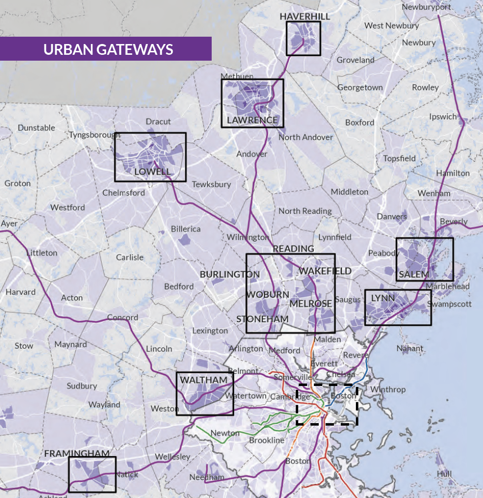
Figure 3: Partial map of urban gateways, as identified by the MBTA (MDOT 2019). The regions are identified with solid-line bounding boxes. The dashed-line bounding box demarcates the region that we identified as the inner city. (Urban gateway not depicted: Brockton, located south of the inner city.)

Our case study integrates many datasets describing travel characteristics in the Greater Boston Area during the weekday morning commute (6-10 am). We consider passenger travel patterns for those who commute from the service region to the inner city (Boston and Cambridge), or those who commute locally within the service region. We define a local commute as either working in the town of residence or in an adjacent town that is also part of the service region. For example, commutes between Salem and Lynn or between Burlington and Melrose are considered local. We use Origin-Destination Employment Statistics from the Longitudinal Employer-Household Dynamics (LODES) datasets provided by the U.S. Census Bureau to approximate the commuting population at a census tract level (U.S. Census Bureau 2017).

We obtain MBTA’s commuter rail network data using MBTA General Transit Specification Feed data (MBTA 2018), while the MOD operator corresponds to all potential direct travel options and first-mile connections in the service region. We construct route choice sets for each passenger type by first executing Yen’s $k$-shortest paths algorithm (Yen 1970). We then include in each passenger type’s route choice set their fastest option of each mode: transit-only, MOD only, hybrid (MOD first mile to transit), and driving (which corresponds to the outside option). We represent the utility of each route option as a linear combination of travel and wait time; incurred costs including fare, gasoline, and parking fees as appropriate; and mode discomfort relative to the convenience of driving. The discount activation categories correspond to town pairs. In other words, a discount might be activated from any town in the service region to the inner city, to an adjacent town that is also part of the service region, or to itself. In total, there are 77 discount activation categories in the case study. We allow each operator to set fares up to a maximum of $10 for base fares, $5 per mile for distance-based markups, and a maximum 0.5 for discount multiplier. Transit-only routes are not eligible for discount, while all others are. Appendix 13 provides more details about the case study.

5.2 Model Validation

First, we will demonstrate that the allied fare-setting model sets route prices in realistic and reasonable ranges from a practical standpoint. Further, we find that the optimal fares intuitively reflect various portfolios of alliance priorities. We vary the objective function coefficients $\bm{\mu}$, i.e., relative weights among the three performance metrics: revenue, passenger utility, and VMT. In particular, we focus on regimes with varying combinations of priorities between revenue and passenger utility (i.e., setting $\mu^{VMT}=0$), as well as between revenue and VMT (i.e., setting $\mu^{PAX}=0$). We do not emphasize regimes that completely exclude revenue as a priority, because they intuitively result in zero fares and are not interesting from an analysis standpoint. Thus, all experiments have $\mu^{REV}>0$. We also do not analyze regimes that vary all three metrics for reasons explained later in this section. Table 6 presents summary statistics about route prices, system utilization, and system-wide performance metrics across the tested priority regimes. Figure 4 depicts optimal fare parameters and discount multipliers, demonstrating the different fare-setting strategies of each regime.

Table 6: Aggregate metrics for different operator priority regimes. System-wide performance metrics are normalized against best possible values. System utilization (util.) is the alliance’s total market share, i.e. the percentage of travelers electing to travel on a transit, MOD, or hybrid option instead of driving a single-occupancy vehicle.

Objective weights			Route price ($)			Performance			System
$\mu^{PAX}$	$\mu^{REV}$	$\mu^{VMT}$	Min.	Mean	Max.	PAX	REV	VMT	util. %
1.0	0	0	$0.00	$0.00	$0.00	100.00%	0.00%	100.00%	50.32%
1.0	0.2	0	$0.00	$0.04	$0.54	99.26%	3.19%	100.59%	50.32%
1.0	0.4	0	$0.18	$4.24	$12.29	80.15%	61.62%	113.01%	45.02%
1.0	0.6	0	$3.63	$7.88	$23.62	70.50%	78.38%	117.89%	40.20%
1.0	0.8	0	$6.63	$10.43	$25.89	64.61%	85.66%	120.39%	37.33%
1.0	1.0	0	$7.04	$12.00	$28.14	59.99%	90.04%	122.35%	35.93%
0.8	1.0	0	$7.17	$13.14	$29.66	56.35%	92.79%	123.81%	34.95%
0.6	1.0	0	$7.47	$15.20	$31.64	51.94%	95.39%	125.33%	32.95%
0.4	1.0	0	$6.91	$16.27	$38.89	46.81%	97.57%	127.13%	31.82%
0.2	1.0	0	$8.59	$18.59	$45.27	40.03%	99.33%	129.17%	29.95%
0	1.0	0	$10.00	$21.58	$60.37	30.91%	100.00%	131.65%	27.65%
0	1.0	0.2	$9.71	$18.28	$42.20	45.90%	97.77%	127.10%	29.95%
0	1.0	0.4	$8.52	$16.41	$36.63	59.59%	89.37%	121.46%	30.97%
0	1.0	0.6	$8.50	$13.02	$25.58	70.54%	76.54%	116.32%	33.99%
0	1.0	0.8	$5.22	$11.13	$21.65	80.62%	56.33%	110.38%	35.17%
0	1.0	1.0	$1.83	$8.39	$14.59	90.11%	29.53%	104.39%	37.83%
0	0.8	1.0	$0.00	$6.77	$10.00	95.40%	10.83%	100.87%	39.48%
0	0.6	1.0	$0.00	$6.67	$9.96	95.58%	10.45%	100.81%	39.54%
0	0.4	1.0	$0.00	$3.70	$6.00	97.63%	6.53%	100.43%	44.04%
0	0.2	1.0	$0.00	$0.00	$0.00	100.00%	0.00%	100.00%	50.32%
0	0	1.0	$0.00	$0.00	$0.00	100.00%	0.00%	100.00%	50.32%

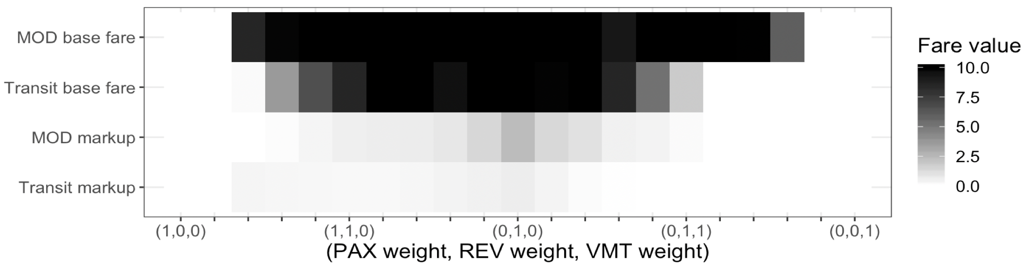
(a) Optimal fare parameter values.

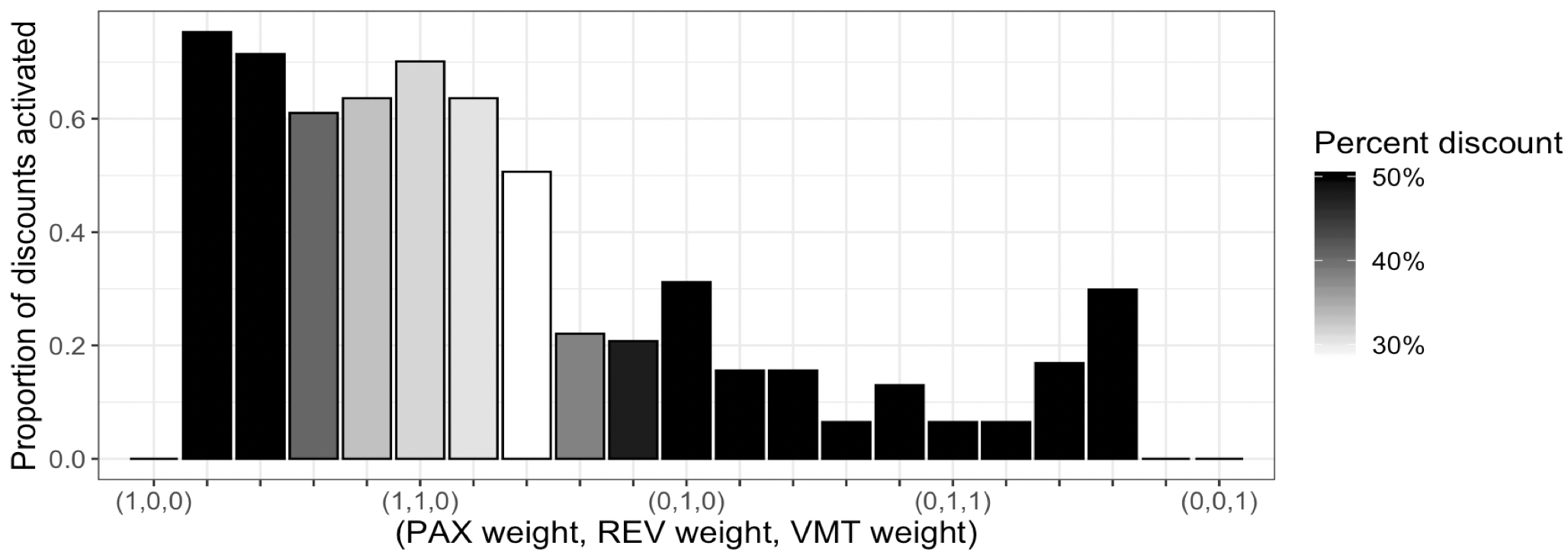
(b) Optimal discount characteristics.

Figure 4: Optimal fares across varying alliance priority regimes.

We extract a few representative solutions from Table 6 and present them in Table 7 alongside real-world fares, and the corresponding ridership values obtained by our model for the real-world fares. We compute the MOD base fare by combining Lyft’s published minimum fare and service fee, and we compute their markup by combining the published markups per unit distance and time, assuming an average vehicle speed of 25 mph (Lyft Inc. 2020). We ignore fare multipliers utilized to manage the two-sided market, since they are outside the scope of this work; note that this may lead to slight undercounting of real MOD fares and slight overcounting of the real ridership. The real-world MBTA commuter rail base fare and markup are interpolated from its zone-based pricing structure, which assigns higher prices to farther zones (MBTA 2020). While all regimes have slightly lower ridership than that under real fares, all benchmarks achieve non-negligible improvements in system-wide metrics. In particular, the REV, REV+PAX, and REV+VMT regimes respectively achieve objective value increases of 47.4%, 5.6%, and 1.8% respectively.

Table 7: Summary statistics of representative priority regimes. REV, REV+PAX, and REV+VMT regimes respectively have objective weights $(\mu^{REV},\mu^{PAX},\mu^{VMT})$ equal to $(1,0,0),(1,1,0),$ and $(1,0,1)$. “% routes discounted” provides the proportion of routes in the system with activated discounts. “Number of travelers” is the total alliance passenger count originating within the alliance service region.

Priority regime	Base fares ($)		Markups ($/mile)		Discount	% routes	Number of
	MOD	Transit	MOD	Transit	Multiplier	discounted	travelers
Real fares	$4.53	$4.50	$1.07	$0.16	0%	0%	25,816
REV	$10.00	$10.00	$2.37	$0.63	50%	31.20%	18,309
REV+PAX	$10.00	$8.50	$0.56	$0.25	31%	70.13%	23,793
REV+VMT	$10.00	$1.83	$0.16	$0.00	50%	6.50%	25,051

As shown in Table 6, each set of priorities induces interpretable optimal prices and passenger decisions. The minimum, mean, and maximum real-world route prices in the service region are respectively $4, $10.23, and $54.46, while those given by our model are in the range $0-$60.37; thus optimal fares are set at the correct order of magnitude across all regimes. Intuitively, route prices are the highest for the revenue maximizing regime, and they decrease gradually as the importance of VMT or passenger utility increases. System-wide performance metrics are normalized against the best possible values across tested regimes, naturally achieved by each metric’s corresponding single-objective optimization. The lowest revenue is achieved in regimes that solely maximize passenger utility or minimize VMT, because very low prices achieve very low revenues, but increase passenger happiness and entice more passengers away from single-occupancy vehicles. Analogously, the highest fares achieve the highest revenue, with more passengers electing to travel outside the system, and lowering overall passenger utility. System-wide outcomes vary smoothly with gradually changing alliance priorities. Note that even under single-objective revenue maximization,, route prices remain in the ballpark of real-world fares. While both base fares and discount multiplier reach their upper limits, the both optimal markups stay in the interior of the allowable range. We attribute the model’s realism to the incorporation of the endogenous passenger choice model into the fare-setting model, as opposed to modeling exogenous demand parametrically. These intuitive observations confirm that our fare-setting model is suitable for generating trustworthy qualitative insights.

At a quick glance, minimizing VMT and maximizing passenger utility seem to achieve similar outcomes in Table 6—lower prices and higher system utilization—raising the question of why it is worth modeling them separately. We turn to Figure 4 to illustrate how each objective yields qualitatively very different designs. As VMT minimization increases in importance (moving from the middle towards the right in Figure 4(a)), the markup is zeroed out, equalizing fares across longer and shorter routes. The elimination of a distance-based markup entices more longer-distance commuters to travel on the allied network, thus lowering VMT. When the system maximizes passenger utility, a more nuanced fare structure emerges to address heterogeneous passenger preferences. All pricing levers are employed: base fares, markups, discount multipliers, and discount activations. Higher markups and base fares are coupled with more numerous discounts across hybrid options, illustrated in the left halves of both Figures 4(a) and 4(b). Thus, prioritization of each objective (PAX versus VMT) results in similar system-wide performance metrics by qualitatively different means. To extract the corresponding fare designs, we consider case studies prioritizing at most one of PAX and VMT at a time, with varying weights for revenue. Section 5.3 further investigates geographic factors.

Finally, note that the variation in system utilization due to allied fare-setting is small compared to the integrated network’s total loads. Before the pandemic, MBTA’s bus load factor during peak hours was already below 75% (Hicks 2017). MBTA commuter rail transported around 120k passengers on an average weekday in 2018 (MBTA 2022), with 81.2% of inbound ridership on peak trains (BRMPO 2012), yielding approximately 49k travelers on MBTA commuter rail during the AM rush. Moreover, approximately 116k daily TNC rides were destined for Boston in 2018, while another 15.3k originated in the alliance service region every day (MDPU 2018). In contrast, the ridership numbers in Table 7 show that the alliance’s ridership under real fares is a small proportion of the entire integrated network and that the system is capable of accommodating all demand redistribution as a result of allied fare-setting. In fact, Table 7 shows that the aggregate alliance ridership is slightly lower than under real fares. Thus, drops on other routes will compensate for the slight ridership increases that may happen on certain routes under our proposed pricing alliance, ensuring that the system-wide transit load factors and MOD detour times are expected to remain largely unchanged as a result of the pricing alliance. We conclude that the linked resource reallocation problem need not be considered, when looking for rapid gains through pricing alliance formation.

5.3 Ensuring Equitable Access through a Refined Income-Aware Model Specification

Our fare-setting model captures passenger’s travel preferences and travel decisions when designing fares, a critical step to satisfying passenger needs. However, different groups of passengers may have very different preferences. Ignoring such differences can lead to inequitable and socially undesirable outcomes. After all, equity is a key driver for integrating on-demand services into public transportation options. Acknowledging this challenge, in this section we further refine our choice model and quantify the impacts of this nuanced model specification on system-wide metrics compared to an aggregated, average-case choice model.

To this end, we augment our case study. Towns targeted for transit expansion by the MBTA in our case study have wide-ranging median household incomes, translating into varying price sensitivities. Affluent travelers’ route choice decisions are less susceptible to changing fares than those of low-income travelers. To partly account for such passenger heterogeneity, we compute a ratio of each town’s median household income to the average of the median household incomes across the entire service region (U.S. Census Bureau 2018). We use this income ratio to scale passengers’ price sensitivities. See Appendix 13 for details.

Table 8: Allied system’s daily morning rush ridership with (Refined) and without (Base) the choice model refinement, their percentage difference (Diff.), real-world ridership (Real), median household income (HHI), and average distance (Dist.) of alliance routes originating in the corresponding town and ending in the inner city.

	HHI	Dist.	REV+PAX			REV			REV+VMT
Town	$K	Miles	Base	Refined	Diff.	Base	Refined	Diff.	Base	Refined	Diff.	Real
Lawrence	41.6	32.4	1585	1982	125%	918	1881	205%	1331	2065	155%	1566
Lowell	52.0	30.8	2000	2525	126%	1285	1565	122%	1852	2633	142%	2115
Lynn	54.6	13.5	3539	3769	107%	2283	2560	112%	3615	3188	88%	4023
Brockton	55.1	24.6	3498	3709	106%	1949	3364	173%	3416	3919	115%	3872
Salem	65.6	18.9	1885	2043	108%	1189	1382	116%	1961	1786	91%	2171
Haverhill	67.6	39.1	1605	1746	109%	1068	1214	114%	1630	1809	111%	1801
Framingham	79.1	26.1	1203	1327	110%	780	936	120%	1093	1117	102%	1198
Waltham	85.7	11.8	1974	1873	95%	1597	1713	107%	2101	1946	93%	2249
Woburn	88.7	14.3	1795	1828	102%	1479	1633	110%	2047	1910	93%	2199
Stoneham	94.8	11.6	761	785	103%	610	691	113%	880	830	94%	948
Wakefield	95.3	13.3	1004	1007	100%	783	889	114%	1140	1076	94%	1228
Melrose	103.7	9.8	810	821	101%	637	711	112%	889	842	95%	949
Burlington	105.4	17.6	1091	1144	105%	975	1053	108%	1264	1193	94%	1340
Reading	112.6	16.6	846	871	103%	703	787	112%	972	927	95%	1038
Winchester	159.5	10.8	197	207	105%	193	198	103%	218	210	96%	227

We compare the allied system ridership across priority regimes and towns under fares corresponding to base (i.e., income-agnostic) as well as refined (i.e., income-aware) choice models. We first calculate fares using the fare-setting model incorporating income-agnostic and income-aware choice models separately, and then evaluate both fare designs by calculating (and reporting in Table 8) ridership using only the income-aware choice model. Due to the use of the income-aware model, the system ridership in the REV+PAX regime increases by 13% on average for the towns with below-average median HHI compared to a less than 2% average increase for the towns with above-average median HHI. While ridership increases across the board due to generally lower fares, the greatest increases occur in Lawrence and Lowell, which are the two towns with the lowest median household incomes. The lower middle-income bracket (Lynn, Brockton, Salem, Haverhill, and Framingham) sees the next-highest ridership increase. Similar trends are observed in the REV regime: ridership increases across all towns due to the fact that higher revenue can be achieved with lower fares and higher volume. The above-average income towns gain ridership by only 10% on average, while the below-average income towns have a 37% gain.

In contrast to the 7% and 23% average ridership gains in REV+PAX and REV regimes, average ridership grows by less than 4% in the REV+VMT regime. But interestingly, this regime has significantly larger ridership increases for longer distance passengers. In particular, the five towns that are farthest from the inner city area—Lawrence, Lowell, Brockton, Haverhill, and Framingham—are the exact five towns with ridership increases. Their average increase is about 25% while the remaining 10 towns see an average 7% drop in ridership. Thus, the REV+VMT regime increases access to the allied network for commuters who are farther from the inner city. Overall, the prioritized system-wide objectives improved by 19.16%, 0.35% and 0.99% respectively for REV+PAX, REV, and REV+VMT regimes compared to the real-world fares.

These results underline the importance of capturing passenger preference heterogeneity to amplify our model’s practical impact. A choice model that reflects passenger preferences more accurately improves system-wide outcomes and especially maximizes passenger benefits. We conclude that our income-aware refined model improves transportation equity for passengers—as compared to the income-agnostic aggregate model—making it a valuable tool for transit agencies to incorporate into strategic decision-making.

5.4 Quantifying the Value of Cooperation

To quantify the value of operator cooperation for operators and passengers, we solve the non-cooperative fare-setting model for all allied priorities depicted in Table 6. In each experiment, the transit operator’s priorities are identical to alliance priorities, whereas the MOD operator always maximizes revenue. Thus, our experiment reflects an assumption that the prospective alliance will adopt the transit operator’s priorities.

Figure 5 depicts the non-cooperative equilibrium fares. Discount multipliers are not included since they are not applicable in the non-cooperative setting. Table 9 compares allied outcomes to corresponding non-cooperative outcomes. In particular, we report the percentage increase in the alliance objective compared to that computed under the non-cooperative setting (transit obj. % inc.), and the percentage increase in MOD operator revenue due to the alliance (MOD rev. % inc.). We also provide the revenue allocations to both operators as determined by the revenue allocation mechanism in Section 2.4. The non-cooperative system utilization and non-cooperative average route prices are also provided for each experiment. Figure 6 illustrates passenger mode choices across all tested regimes for both allied and non-cooperative fares.

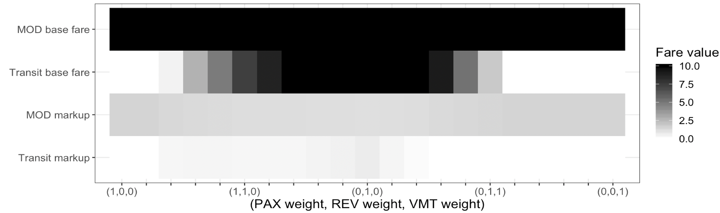
Figure 5: Non-cooperative fare parameters for different transit operator priorities.

Table 9: Allied vs. non-cooperative outcomes. Transit operator’s priorities represented as $\bm{\mu}_{TR}$.

Transit obj. weights			Transit obj.	MOD rev.	MOD allied	Transit allied	System	Route price
$\mu_{TR}^{PAX}$	$\mu_{TR}^{REV}$	$\mu_{TR}^{VMT}$	% inc.	% inc.	rev. alloc.	rev. alloc.	util. %	($) Mean
1.0	0	0	9.60%	0.00%	$501.90K	-$501.90K	35.01%	$12.83
1.0	0.2	0	6.87%	0.00%	$501.90K	-$501.90K	35.01%	$12.83
1.0	0.4	0	4.93%	0.00%	$487.91K	$1848.89K	32.41%	$13.45
1.0	0.6	0	4.80%	0.00%	$479.04K	$2337.68K	30.46%	$14.78
1.0	0.8	0	5.45%	0.00%	$473.18K	$2624.27K	29.21%	$15.83
1.0	1.0	0	7.57%	0.00%	$468.14K	$2824.63K	28.16%	$16.96
0.8	1.0	0	27.71%	0.00%	$465.06K	$2940.94K	27.39%	$17.77
0.6	1.0	0	5.82%	0.00%	$462.29K	$3022.50K	26.70%	$18.54
0.4	1.0	0	1.31%	0.00%	$460.45K	$3101.99K	26.43%	$18.66
0.2	1.0	0	0.54%	1.04%	$463.61K	$3173.57K	26.00%	$18.97
0	1.0	0	0.33%	1.33%	$462.79K	$3195.02K	25.65%	$19.24
0	1.0	0.2	1.55%	4.42%	$481.71K	$3108.48K	26.66%	$18.50
0	1.0	0.4	0.52%	0.00%	$465.54K	$2839.52K	27.50%	$18.07
0	1.0	0.6	0.37%	4.34%	$492.25K	$2376.74K	28.67%	$17.40
0	1.0	0.8	0.51%	0.00%	$482.97K	$1573.28K	31.13%	$15.33
0	1.0	1.0	0.54%	0.00%	$494.38K	$591.27K	33.48%	$13.76
0	0.8	1.0	0.60%	0.00%	$501.90K	-$105.59K	35.01%	$12.83
0	0.6	1.0	0.73%	0.00%	$501.90K	-$119.73K	35.01%	$12.83
0	0.4	1.0	0.92%	0.00%	$501.90K	-$262.97K	35.01%	$12.83
0	0.2	1.0	1.36%	0.00%	$501.90K	-$501.90K	35.01%	$12.83
0	0	1.0	1.90%	0.00%	$501.90K	-$501.90K	35.01%	$12.83

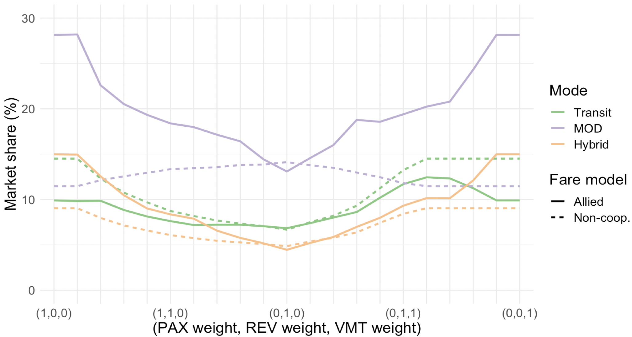
Figure 6: Market shares by mode across priority regimes for allied and non-cooperative fare-setting models.

Figure 5 illustrates that the MOD operator’s revenue-maximizing strategy remains relatively constant, regardless of the transit operator’s priorities. Still, when the transit operator prioritizes VMT minimization or passenger benefits maximization, the MOD operator selects higher fare parameters (mainly through higher markups) than in the corresponding allied settings. Thus, the average route price (Route price ($) Mean) columns in Tables 6 and 9 show that the non-cooperative average route prices are higher than average allied route prices in every regime except for the one where the transit operator only prioritizes revenue.

In scenarios that partially maximize passenger benefits or minimize VMT, the alliance sets MOD fare parameters lower than in the non-cooperative regime (Figure 4(a) vs. 5). Figure 6 shows that MOD-only market shares decrease and hybrid market shares increase in the non-cooperative regime as passenger benefits or VMT are increasingly prioritized. We can conclude that, although fewer passengers utilize MOD-only options in non-cooperative scenarios where the transit operator is VMT- or passenger-oriented, a higher volume of passengers selects hybrid options due to the very low (or free) transit fares observed in Figure 5. Thus, the MOD operator earns more revenue in those non-cooperative scenarios in which the transit operator is more altruistic. This is reflected in the revenue allocation mechanism: observe in Table 9 that the MOD operator earns strictly more revenue in almost all regimes where the transit operator is not solely a revenue maximizer, even though the system as a whole generates strictly less total revenue, as seen in comparison with Table 6. The revenue allocation mechanism ensures that the MOD operator receives their non-cooperative earnings, despite the lower MOD fares that the alliance sets to achieve lower VMT or higher passenger benefits. This in turn reduces the transit’s revenue allocation as high VMT or low passenger benefits are increasingly penalized. On the other hand, the transit operator always strictly improves its objective of optimizing total system-wide performance, however it chooses to define it. As a result, the MOD operator interestingly finds it in its interest to adopt transit’s priorities as transit increasingly diverges from revenue maximization. In other words, the revenue-maximizing MOD operator would not prefer a revenue-maximizing alliance. In fact, the MOD operator would benefit most from total altruism on transit’s side (an exclusive focus on either passenger utility or VMT reduction). Passengers win due to the strictly lower prices and higher system utilization that result from such alliances.

The transit operator must ultimately set the ceiling in terms of the price they are willing to pay for the alliance benefits. Table 9 shows that the transit agency runs a deficit to appease the MOD operator if its revenue emphasis is too low. A deficit alone might not be enough to dissuade the transit agency from participating in the alliance: as we have noted, every public transit mode operates at a loss, especially on-demand options (Kane, Tomer, and Puentes 2016). To weigh the financial implications of an alliance, the agency may compare the magnitude of the loss to the cost of the analogous MOD system operated by transit on their own in the absence of outsourcing through an alliance. Oftentimes, transit agencies also receive grants to fund pricing alliances (Federal Transp. Administration 2016), and the daily deficit rate can be compared to the grant award amount and intended duration. To enable a daily deficit rate that keeps pace with financial resources over time, the transit agency may propose to reset overall performance metric goals to induce different optimal fares, or to adjust the geographic and/or temporal scope of the alliance. In the end, each transit agency is expected to choose the trade-off point between its financial, passenger-focused, and environmental goals that most closely aligns with their overall policy and various practical and financial constraints. Regardless, our allied and non-cooperative fare-setting models together with our revenue allocation mechanism jointly provide a toolkit usable by transit agencies to weigh these trade-offs as they evaluate a potential pricing alliance.

6 Conclusions, Limitations and Future Directions

We contribute a pricing alliance design framework to enable incentive-aligned collaboration between transit agencies and MOD operators. Our allied fare-setting model captures the interdependent decisions of passengers and operators, allowing the alliance to maximize benefits for all stakeholders across the integrated network. The prescriptive pricing framework can be generalized to different types of large-scale alliances with varying MOD operators, service populations, fare structures, service goals, and network configurations. We accomplish large scale by developing a tractable two-stage fare-setting formulation equivalent to the original mixed-integer non-convex optimization problem, which we then solve with a tailored SOS2 coordinate descent approach. From a technical standpoint, our approach selects consistently and significantly higher quality solutions than benchmarks based on Bayesian Optimization, enabling additional system-wide benefits worth tens of thousands dollars per day over the service region. Practically speaking, the high quality solutions from our allied fare-setting model together with our dedicated revenue allocation mechanism work together to align revenue-oriented MOD operators with transit goals of passenger utility and single-occupancy VMT reduction. In other words, cooperative pricing results in win-win-win outcomes for passengers, MOD operators, and transit agencies. Finally, the income-aware nuanced version of our fare-setting model helps enhance passenger equity-related goals: by tuning passenger route choice models, the alliance can prioritize lower fares and higher utilization for low-income or long-distance commuters.

Our analysis is based on a few assumptions which can be relaxed in future work. We assumed that the MOD operator serves as a contractor to the transit agency and agrees to set static fares for trips in the integrated system. While this is one good way to ensure public sector prices are transparently communicated, it may also be possible to set fare schemes that allow MOD operators, especially TNCs, to maintain their dynamic prices, perhaps through the transit operator subsidizing the cost of a passenger’s trip up to a fixed dollar amount. Additionally, we model average-case travel times over a fixed set of route options for the MOD operator’s portion of the network to represent average-case operations, which simplifies their typically dynamic routing scheme. In other words, we consider the case where the alliance sets one permanent fare scheme that is optimized for average-case performance. Future research may consider optimizing for the worst-case performance, and/or integrating dynamic routing into the fare-setting model if the alliance prefers dynamic fares, requiring the integration of two complex problem classes. Finally, we did not incorporate joint resource reallocation into the pricing scheme, due to the observation that the system is capable of accommodating all demand re-distributions attributed to changing prices. This assumption works well for our case study over the Greater Boston Area because the allied system’s ridership is a small fraction of the larger service region with a high-capacity existing network. Future research could consider relaxing this assumption to generalize the analysis by jointly modeling the capacity allocation and pricing decisions.

This material is based upon work supported by the National Science Foundation under Grant no. 1122374.

7 Proof of Lemma 2.1: Two-stage Decomposition is Equivalent to Full Formulation

Given an optimal solution from each formulation, we construct a feasible solution for the other with the same objective value. In this section, we introduce the following notation for a non-discounted route price $r\in\mathcal{R}$, for expositional brevity:

$$\sigma_{r}(\bm{\beta})=\sum_{k\in\mathcal{O}_{r}}(\beta_{k}^{0}+\Delta_{rk}\cdot\beta_{k}^{\Delta}).$$ (35)

PADP-FS2SD $\to$ PADP-FS.

Let $(\bm{\beta}^{2SD},\Lambda^{2SD},\bm{x}^{2SD},\bm{s}^{2SD},\bm{w}^{2SD},\bm{p}^{2SD})$ be an optimal solution to the PADP-FS2SD model with objective value $z^{2SD}$. We construct the following solution to the PADP-FS model.

$$\begin{cases}\bm{\beta}^{FS}=\bm{\beta}^{2SD}\\ \Lambda^{FS}=\Lambda^{2SD}\\ \bm{x}^{FS}=\bm{x}^{2SD}\\ \bm{s}^{FS}=\bm{s}^{2SD}\\ \bm{p}^{FS}=\bm{p}^{2SD}\\ \end{cases}$$ (36)

We demonstrate feasibility of (36) to the PADP-FS model.

• $\bm{x}^{FS}$ are binary by construction.

• Constraints (6) and (7) hold by construction.

• Constraints (8) and (9) are feasible due to constraints (18), (21), and (22). For a given $i\in\mathcal{N}$, constraints (18) and (22) ensure that

  $$s_{ir}^{FS}\propto\exp(u_{ir}+\alpha_{i}\cdot p_{r}^{FS}) \forall r\in\mathcal{R}_{i},\text{ and }$$

  $$s_{i0}^{FS}\propto\exp(u_{i0}).$$

  Constraint (21) forces each $s_{ir}$ and $s_{i0}$ to be normalized by $\exp(u_{i0})+\sum_{r\in\mathcal{R}_{i}}\exp(u_{ir}+\alpha_{i}\cdot p_{r}^{FS}).$ The result follows.

• Constraints (10) - (12) hold by definition of $\mathcal{B}$ and $\mathcal{L}.$

Finally, to show that solution (36) has the same objective value as $z^{2SD},$ we must only prove that $p_{r}^{FS}\cdot s_{ir}^{FS}=w_{ir}^{2SD}$ for all $i\in\mathcal{N}$ and $r\in\mathcal{R}_{i},$ which follows directly from Constraints (19) and (23).

PADP-FS $\to$ PADP-FS2SD.

Let $(\bm{\beta}^{FS},\Lambda^{FS},\bm{p}^{FS},\bm{s}^{FS},\bm{x}^{FS})$ be an optimal solution to the PADP-FS model with objective value $z^{FS}$. We construct the following solution to the PADP-FS2SD model.

$$\begin{cases}\bm{\beta}^{2SD}=\bm{\beta}^{FS}\\ \Lambda^{2SD}=\Lambda^{FS}\\ \bm{x}^{2SD}=\bm{x}^{FS}\\ \bm{s}^{2SD}=\bm{s}^{FS}\\ w_{ir}^{2SD}=p_{r}^{FS}\cdot s_{ir}^{FS}&\forall i\in\mathcal{N},r\in\mathcal{R}_{i}\\ \bm{p}^{2SD}=\bm{p}^{FS}\end{cases}$$ (37)

First we demonstrate the feasibility of (37) to PADP-FS2SD.

• $\bm{s}^{2SD}$, $\bm{w}^{2SD}$ and $\bm{p}^{2SD}$ are non-negative and $\bm{x}^{2SD}$ are binary by construction.

• Constraints (18) and (22): Consider any $i\in\mathcal{N}.$ For $r\in\mathcal{R}_{i}\setminus\mathcal{R}^{DE},$ and by expressions (8) and (9),

  $$\gamma_{ir}(\bm{\beta}^{2SD},0)\cdot s_{ir}^{2SD} =\gamma_{ir}(\bm{\beta}^{FS},0)\cdot s_{ir}^{FS}$$

  $$=\frac{\exp(u_{i0})}{\exp(u_{ir}+\alpha_{i}\cdot p_{r}^{FS})}\cdot\frac{\exp(u_{ir}+\alpha_{i}\cdot p_{r}^{FS})}{u_{i0}+\sum_{s\in\mathcal{R}_{i}}\exp(u_{is}+\alpha_{i}\cdot p_{s}^{FS})}$$

  $$=\frac{\exp(u_{i0})}{u_{i0}+\sum_{s\in\mathcal{R}_{i}}\exp(u_{is}+\alpha_{i}\cdot p_{s}^{FS})}$$

  $$=s_{i0}^{FS}=s_{i0}^{2SD}.$$

  Thus constraints (22) are satisfied. Now, consider any $a\in\mathcal{A}$ with $r\in\mathcal{R}_{ia}.$ If $x_{a}^{2SD}=0$, then we can use the exact same argument as above to confirm that $\gamma_{ir}(\bm{\beta}^{2SD},0)\cdot s_{ir}^{2SD}=s_{i0}^{2SD}$ again holds. Since

  $$\gamma_{ir}(\bm{\beta}^{2SD},\Lambda^{2SD})\cdot s_{ir}^{2SD} \leq\gamma_{ir}(\bm{\beta}^{2SD},0)\cdot s_{ir}^{2SD}=s_{i0}^{2SD}$$

  $$\leq\gamma_{i0}(\bm{\beta}^{2SD},0)$$

  $$\leq\gamma_{i0}(\bm{\beta}^{2SD},0)+\gamma_{ir}(\bm{\beta}^{2SD},\Lambda^{2SD})\cdot s_{ir}^{2SD}$$

  $$=\gamma_{ir}(\bm{\beta}^{2SD},\Lambda^{2SD})\cdot s_{ir}^{2SD}+M_{ir}^{s}\cdot(1-x_{a}^{2SD}),$$

  the constraints hold. A similar argument applies when $x_{a}^{2SD}=1.$

• Constraints (19) and (23): For any $i\in\mathcal{N}$, Constraints (23) hold by construction for all $r\in\mathcal{R}_{i}\setminus\mathcal{R}^{DE}.$ For $a\in\mathcal{A}$ with $r\in\mathcal{R}_{ia},$ we have $w_{ir}^{2SD}=p_{r}^{2SD}\cdot s_{ir}^{2SD}$ regardless of the value of $x_{a}^{2SD}.$ If $x_{a}^{2SD}=0,$ then

  $$(1-\Lambda^{2SD})\cdot\sigma_{r}(\bm{\beta}^{2SD})\cdot s_{ir}^{2SD} \leq w_{ir}^{2SD}=\sigma_{r}(\bm{\beta}^{2SD})\cdot s_{ir}^{2SD}$$

  $$=(1-\Lambda^{2SD})\cdot\sigma_{r}(\bm{\beta}^{2SD})\cdot s_{ir}^{2SD}+\Lambda^{2SD}\cdot\sigma_{r}(\bm{\beta}^{2SD})\cdot s_{ir}^{2SD}$$

  $$\leq(1-\Lambda^{2SD})\cdot\sigma_{r}(\bm{\beta}^{2SD})\cdot s_{ir}^{2SD}+\Lambda^{2SD}\cdot\sigma_{r}(\bm{\beta}^{2SD})$$

  $$=(1-\Lambda^{2SD})\cdot\sigma_{r}(\bm{\beta}^{2SD})\cdot s_{ir}^{2SD}+M_{ir}^{w}\cdot(1-x_{a}^{2SD}),$$

  and hence constraints (19) hold. A similar argument applies when $x_{a}^{2SD}=1.$

• Constraints (21): Consider any $i\in\mathcal{N}.$ By expressions (8) and (9),

  $$s_{i0}^{2SD}+\sum_{r\in\mathcal{R}_{i}}s_{ir}^{2SD} =s_{i0}^{FS}+\sum_{r\in\mathcal{R}_{i}}s_{ir}^{FS}$$

  $$=\frac{\exp(u_{i0})}{\exp(u_{i0})+\sum_{s\in\mathcal{R}_{i}}\exp(u_{is}+\alpha_{i}\cdot p_{s}^{FS})}+$$

  $$\qquad\sum_{r\in\mathcal{R}_{i}}\frac{\exp(u_{ir}+\alpha_{i}\cdot p_{r}^{FS})}{\exp(u_{i0})+\sum_{s\in\mathcal{R}_{i}}\exp(u_{is}+\alpha_{i}\cdot p_{s}^{FS})}$$

  $$=1.$$

• Constraints (24) and (25) hold by construction.

• Constraints $\bm{\beta}\in\mathcal{B}$ and $\Lambda\in\mathcal{L}$ hold by construction.

Now we show that solution (37) to Formulation PADP-FS2SD has the same objective value of $z^{FS}$.

$$z^{2SD} =\sum_{i\in\mathcal{N}}N_{i}\cdot\Big{[}\mu^{PAX}\cdot(u_{i0}+\sum_{r\in\mathcal{R}_{i}}(u_{ir}+\alpha_{i}\cdot p_{r}^{2SD})+\mu^{REV}\cdot\sum_{r\in\mathcal{R}_{i}}w_{ir}^{2SD}-\mu^{VMT}\cdot(\Delta_{i0}\cdot s_{i0}^{2SD})\Big{]}$$

$$=\sum_{i\in\mathcal{N}}N_{i}\cdot\Big{[}\mu^{PAX}\cdot(u_{i0}+\sum_{r\in\mathcal{R}_{i}}(u_{ir}+\alpha_{i}\cdot p_{r}^{2SD})+\mu^{REV}\cdot\sum_{r\in\mathcal{R}_{i}}p_{r}^{2SD}\cdot s_{ir}^{2SD}-\mu^{VMT}\cdot(\Delta_{i0}\cdot s_{i0}^{2SD})\Big{]}$$

$$=\sum_{i\in\mathcal{N}}N_{i}\cdot\Big{[}\mu^{PAX}\cdot(u_{i0}+\sum_{r\in\mathcal{R}_{i}}(u_{ir}+\alpha_{i}\cdot p_{r}^{FS})+\mu^{REV}\cdot\sum_{r\in\mathcal{R}_{i}}p_{r}^{FS}\cdot s_{ir}^{FS}-\mu^{VMT}\cdot(\Delta_{i0}\cdot s_{i0}^{FS})\Big{]}$$

$$=z^{FS}$$

8 Non-cooperative Fare-setting Game and Iterated Best Response Algorithm

To benchmark the solutions of our allied fare-setting model, we formulate the non-cooperative fare-setting problem between a transit operator and an MOD operator. When they are not allied, each operator can only make fare-setting decisions over their portion of the integrated network. The discount activation decision is not applicable in this context, and operators set their own fare parameters so as to optimize their prioritized performance metrics over the integrated network, subject to endogenous passenger decisions.

First we introduce new notation. Let $\bm{\mu}_{k}=(\mu_{k}^{PAX},\mu_{k}^{REV},\mu_{k}^{VMT})$ be the relative priority weights of operator $k\in\mathcal{O}$ for each system-wide performance metric. For a given $k\in\mathcal{O}$, let $-k$ indicate the other operator, i.e. the singleton $-k\in\mathcal{O}\setminus\{k\}.$ Each operator sets fare parameters $\bm{\beta}_{k}=(\beta_{k}^{0},\beta_{k}^{\Delta})$. Let $\mathcal{B}_{k}:=[\beta_{min}^{0},\beta_{max}^{0}]\times[\beta_{min}^{\Delta},\beta_{max}^{\Delta}]$ be the set of valid fare parameters that operator $k$ can set. Let $s_{i0}(\bm{\beta})$ and $s_{ir}(\bm{\beta})$ respectively denote the market shares of the outside option and of route $r\in\mathcal{R}_{i}$ for passenger type $i\in\mathcal{N}$, as functions by both operators’ fare parameters $\bm{\beta}.$

$$s_{ir}(\bm{\beta})=\frac{\exp(u_{ir}+\alpha_{i}\cdot\sigma_{r}(\bm{\beta}))}{\exp(u_{i0})+\sum_{s\in\mathcal{R}_{i}}\exp(u_{is}+\alpha_{i}\cdot\sigma_{s}(\bm{\beta}))} i\in\mathcal{N},r\in\mathcal{R}_{i}$$

$$s_{i0}(\bm{\beta})=\frac{\exp(u_{i0})}{\exp(u_{i0})+\sum_{s\in\mathcal{R}_{i}}\exp(u_{is}+\alpha_{i}\cdot\sigma_{s}(\bm{\beta}))} i\in\mathcal{N}$$

Let $\hat{\bm{\beta}}_{-k}$ denote the fixed fare parameter decisions of operator $-k$. Then $\sigma_{r}(\bm{\beta}_{k};\hat{\bm{\beta}}_{-k})$ denotes the non-discounted price of route $r\in\mathcal{R}$ as a function of the fare parameter decisions of operator $k,$ parameterized by the fixed decisions of operator $-k$, where $\sigma_{r}$ is originally defined in Equation (35). Similarly, $s_{ir}(\bm{\beta}_{k};\hat{\bm{\beta}}_{-k})$ and $s_{i0}(\bm{\beta}_{k};\hat{\bm{\beta}}_{-k})$ represent market shares as functions of the fare parameter decisions of operator $k$, given fixed decisions of operator $-k$. Formulation PADP-NC is the non-cooperative fare setting model of operator $k$.

$$(\text{PADP-NC})\quad\max_{\bm{\beta}_{k}\in\mathcal{B}_{k}}W_{k}(\bm{\beta}_{k};\hat{\bm{\beta}}_{-k})\quad\equiv\quad\max_{\bm{\beta}_{k}\in\mathcal{B}_{k}}\quad\sum_{i\in\mathcal{N}}N_{i}\cdot\Big{[} \mu_{k}^{PAX}\cdot\big{(}u_{i0}+\sum_{r\in\mathcal{R}_{i}}(u_{ir}+\alpha_{i}\cdot\sigma_{r}(\bm{\beta}_{k};\bm{\hat{\beta}}_{-k}))\big{)}+$$

$$\mu_{k}^{REV}\cdot\sum_{r\in\mathcal{R}_{i}}\sigma_{r}(\bm{\beta}_{k};\bm{\hat{\beta}}_{-k})\cdot s_{ir}(\bm{\beta}_{k};\bm{\hat{\beta}}_{-k})-$$

$$\mu_{k}^{VMT}\cdot(\Delta_{i0}\cdot s_{i0}(\bm{\beta}_{k};\bm{\hat{\beta}}_{-k}))\Big{]}$$

An operator’s non-cooperative fare-setting model is a simplified version of the allied fare-setting model, with more restricted decisions. Operator $k$ sets their fare parameters within allowable bounds to maximize system-wide benefits over the integrated network, subject to the induced passenger decisions and for given fare parameters set by the other operator. Each operator’s model has two decision variables: their base fare and their distance-based markup. Fare parameters $\bm{\beta}$ must satisfy condition (38) below to be considered a solution to the non-cooperative fare setting problem.

$$\bm{\beta}_{k}=\arg\max_{\bm{\beta}_{k}^{\prime}\in\mathcal{B}_{k}}W_{k}(\bm{\beta}_{k}^{\prime};\bm{\beta}_{-k})\qquad k\in\mathcal{O}$$ (38)

When fare parameters $\bm{\beta}$ satisfy condition (38), they define a Nash equilibrium (NE), or more precisely, a pure strategy Nash equilibrium. Fare parameters form an NE when neither operator can unilaterally change their pricing strategy to improve their own objective, given the fare parameters set by the other operator. We compute an NE using an iterated best response algorithm, which takes turns alternating between each operator’s optimal fare parameters computation in response to their competitor’s fixed fare parameters, until convergence.

A pure strategy Nash equilibrium to the non-cooperative fare-setting game is a set of fares such that each operator’s decision is the optimal response given the other operator’s fare parameters. An iterated best response algorithm randomly initializes the fare parameters and lets each operator take turns setting their best response. The algorithm converges when neither operator can gain by changing their response (Fudenberg and Tirole 1991).

Algorithm 4 Iterated best response for non-cooperative fare setting

1:procedure Iterated Best Response($\epsilon$)

2:     $\bm{\beta}_{k}\leftarrow$ uniform draw from $\mathcal{B}_{k}$ for each $k\in\mathcal{O}$

3:     $objPrev_{k}\leftarrow-\infty$ for each $k\in\mathcal{O}$

4:     $objCur_{k}\leftarrow W_{k}(\bm{\beta})$ for each $k\in\mathcal{O}$

5:     while $\max_{k\in\mathcal{O}}(objCur_{k}-objPrev_{k})>\epsilon$ do

6:         for $k\in\mathcal{O}$ do

7:              $objPrev_{k}\leftarrow objCur_{k}$

8:              $obj\leftarrow\max_{\bm{\beta}_{k}^{\prime}\in\mathcal{B}_{k}}W_{k}(\bm{\beta}_{k}^{\prime};\bm{\beta}_{-k})$

9:              if $obj>objCur_{k}$ then

10:                  $objCur_{k}\leftarrow obj$

11:                  $\beta_{k}\leftarrow\arg\max_{\bm{\beta}_{k}^{\prime}\in\mathcal{B}_{k}}W_{k}(\bm{\beta}_{k}^{\prime};\bm{\beta}_{-k})$                             

12:     return $\bm{\beta}$

In general, without proof of existence of a Nash equilibrium, Algorithm 4 is not guaranteed to converge, let alone to the same $\bm{\beta}$ in the face of random initializations. To prevent infinite oscillation, a maximum iteration limit can potentially be implemented. Yet, in all runs of our computational experiments performed when generating Table 9, a unique NE was always obtained across the 10 random initializations in a given row of the table.

9 Proof of Lemma 2: Revenue Allocation Mechanism

Proof of Lemma (2.2a):

The MOD operator participates in the alliance whenever they can earn at least as much revenue by cooperating with the transit agency as they can otherwise. By construction,

$$\Phi_{MOD}((f_{k}(\bm{\beta}^{nc}))_{k\in\mathcal{O}},f(\bm{\beta}^{a},\Lambda^{a}))=f_{MOD}(\bm{\beta}^{nc})+\big{(}\tfrac{\delta}{2}\big{)}^{+}\geq f_{MOD}(\bm{\beta}^{nc}),$$

so the result follows.

Proof of Lemma (2.2b):

In the case that allied revenue exceeds combined non-cooperative revenue, we show that the allocation is a Nash bargaining solution, which is a classic payment rule guaranteeing properties of Pareto efficiency, symmetry, scale invariance, and independence of irrelevant alternatives.

We frame the alliance revenue allocation problem as a collective bargaining problem. Let the disagreement outcome be the operator revenues resulting from non-cooperation, $\bm{d}=(f_{k}(\bm{\beta}^{nc}))_{k\in\mathcal{O}}$. Let $\mathcal{X}$ be the set of all revenue allocations such that each operator receives at least their disagreement outcome, and such that the sum of revenue allocations does not exceed allied revenue $p=f(\bm{\beta}^{a},\Lambda^{a})$.

$$\mathcal{X}(\bm{d},p):=\Big{\{}\big{(}a_{k}\big{)}_{k\in\mathcal{O}}:a_{k}\geq d_{k},\forall k\in\mathcal{O};\,\sum_{k\in\mathcal{O}}a_{k}\leq p\Big{\}}$$

Let $\mathcal{F}$ be the set of all such allocation problems, with each $(\bm{d},p)\in\mathcal{F}$ corresponding to a different allocation problem (i.e., a different potential alliance). We seek an allocation solution function $\Phi:\mathcal{F}\to\mathcal{X}$ that allocates the available profit according to the axioms of Pareto efficiency, symmetry, scale invariance, and independence of irrelevant alternatives. It is known that Nash bargaining solutions – which satisfy the above axioms– exactly coincide with optimal solutions to optimization problem (39).

$$\max_{\bm{a}\in\mathcal{X}(\bm{d},p)}\prod_{k\in\mathcal{O}}(a_{k}-d_{k})$$ (39)

Expression (40) clearly solves (39).

$$d_{k}+\frac{p-\sum_{k\in\mathcal{O}}d_{k}}{2}=f_{k}(\bm{\beta}^{nc})+\frac{\delta}{2}\equiv\Phi_{k}(\bm{d},p),\quad\forall k\in\mathcal{O}$$ (40)

To establish the core property, we point to Lemma (2.2a), as well as the fact that $\Phi_{TR}(\bm{d},p)\geq f_{TR}(\bm{\beta}^{nc})$ in the case that $\delta\geq 0$. This proves Lemma (2.2a).

10 SOS2 Coordinate Descent Subroutines

This section specifies subroutines of SOS2 Coordinate Descent, presented in Algorithm 2. The subroutine Search Directions provides a comprehensive ordered list of search directions that can be multidimensional and/or randomized or neither. The subroutine Generate Anchors computes an ordered set of evenly spaced SOS2 anchors along the specified search direction. In case of a multidimensional search direction, we determine the range of slopes that will ensure that the line spans the selected dimension, and sample uniformly from that range.

Algorithm 5 Subroutines for SOS2 Coordinate Descent

1:procedure Search Directions($random$, $multidim$)

2:    if $multidim$ then

3:        $searchDirs\leftarrow\{(\beta^{0}_{TR},\beta^{\Delta}_{TR}),\>(\beta^{0}_{MOD},\beta^{\Delta}_{MOD}),\>\Lambda\}$  // index names of $\bm{y}$

4:    else

5:        $searchDirs\leftarrow\{\beta^{0}_{TR},\>\beta^{\Delta}_{TR},\>\beta^{0}_{MOD},\>\beta^{\Delta}_{MOD},\>\Lambda\}$     

6:    if $random$ then

7:        $searchDirs\leftarrow\text{\sc shuffle}(searchDirs)$  // randomly permutes the set $searchDirs$     

8:    return $searchDirs$

9:procedure Generate Anchors($(\bm{\beta},\Lambda)$, $searchDir$, $D$)

10:    if $searchDir\in\{(\beta^{0}_{k^{\prime}},\beta^{\Delta}_{k^{\prime}})\,:\,k^{\prime}\in\mathcal{O}\}$ then  // if $searchDir$ is multidimensional

11:        $\beta^{0}_{k},\beta^{\Delta}_{k}\leftarrow searchDir$

12:        if Unif$(0,1)<0.5$ then  // select spanning dimension

13:           $(x,x_{min},x_{max}),(y,y_{min},y_{max})\leftarrow(\beta^{0}_{k},\beta^{0}_{min},\beta^{0}_{max}),(\beta^{\Delta}_{k},\beta^{\Delta}_{min},\beta^{\Delta}_{max})$

14:        else

15:           $(x,x_{min},x_{max}),(y,y_{min},y_{max})\leftarrow(\beta^{\Delta}_{k},\beta^{\Delta}_{min},\beta^{\Delta}_{max}),(\beta^{0}_{k},\beta^{0}_{min},\beta^{0}_{max})$         

16:        if $x==0$ then  // determine valid slopes for spanning affine lines

17:           $m_{min}\leftarrow\tfrac{y_{min}-y}{x_{max}-x}$;   $m_{max}\leftarrow\tfrac{y_{max}-y}{x_{max}-x}$

18:        else if $x==x_{max}$ then

19:           $m_{min}\leftarrow\tfrac{y_{max}-y}{x_{min}-x}$;   $m_{max}\leftarrow\tfrac{y_{min}-y}{x_{min}-x}$

20:        else

21:           $m_{min}\leftarrow\max\{\tfrac{y_{max}-y}{x_{min}-x},\tfrac{y_{min}-y}{x_{max}-x}\}$;   $m_{max}\leftarrow\min\{\tfrac{y_{min}-y}{x_{min}-x},\tfrac{y_{max}-y}{x_{max}-x}\}$  // see Figure 7         

22:        $m\leftarrow\text{Unif}(m_{min},m_{max})$;   $b\leftarrow y-m\cdot x$;   $\delta_{x}=x_{max}-x_{min}$  // slope of spanning affine line

23:        $anchors\leftarrow\{(x_{min}+\tfrac{i-1}{D-1}\cdot\delta_{x},b+m\cdot(x_{min}+\tfrac{i-1}{D-1}\cdot\delta_{x}),\beta_{-k}^{0},\beta_{-k}^{\Delta},\Lambda)\,:\,i\in\{1,\dots,D\}\}$

24:    else

25:        if $searchDir==\Lambda$ then

26:           $maxVal\leftarrow\Lambda^{max};\,minVal\leftarrow\Lambda^{min}$

27:        else if $searchDir$ in $\{\beta^{0}_{k}\,:\,k\in\mathcal{O}\}$ then

28:           $maxVal\leftarrow\beta^{0}_{max};\,minVal\leftarrow\beta^{0}_{min}$

29:        else

30:           $maxVal\leftarrow\beta^{\Delta}_{max};\,minVal\leftarrow\beta^{\Delta}_{min}$         

31:        $anchors\leftarrow\{(minVal+\tfrac{i-1}{D-1}\cdot(maxVal-minVal),(\bm{\beta},\Lambda)\setminus\{searchDir\})\,:\,i\in\{1,\dots,D\}\}$     

32:    Insert $(\bm{\beta},\Lambda)$ into the ordered set $anchors$

33:    return $anchors$

Figure 7 visualizes the computation of the slope range in lines (16)-(21) of the Generate Anchors procedure. The most negative slope of a line passing through the current solution is determined by the maximum of the slopes of the two line segments connecting the current solution to the upper left and bottom right corners of the diagram. Similarly, the most positive slope is determined by the minimum of the slopes of the two line segments connecting the current solution to the lower left and upper right corners.

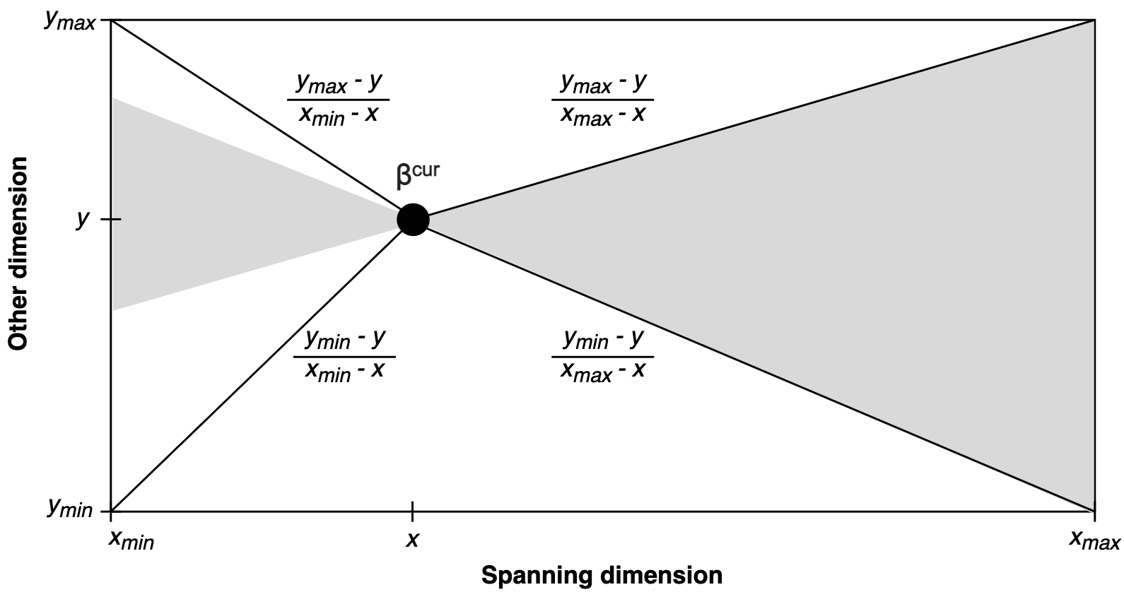
Figure 7: Computing the range of slopes such that the selected dimension is spanned.

11 Performance of Algorithm Components

In this section, we examine the performance of individual components of the algorithm.

Figure 8 illustrates the distribution of solution times in seconds for the second-stage model. Each calculation of $W$, which requires solving the second-stage model once, needs on average 5.7 seconds of CPU time, which is fast enough to be useful, but slow enough to warrant judicious selection of candidate first-stage solution points to evaluate. Each of the 31,553 observations was obtained in under one minute. The observations were aggregated across all solutions of the second-stage model represented in the paper, including runs of SOS2-CD, BF-CD, and BO.

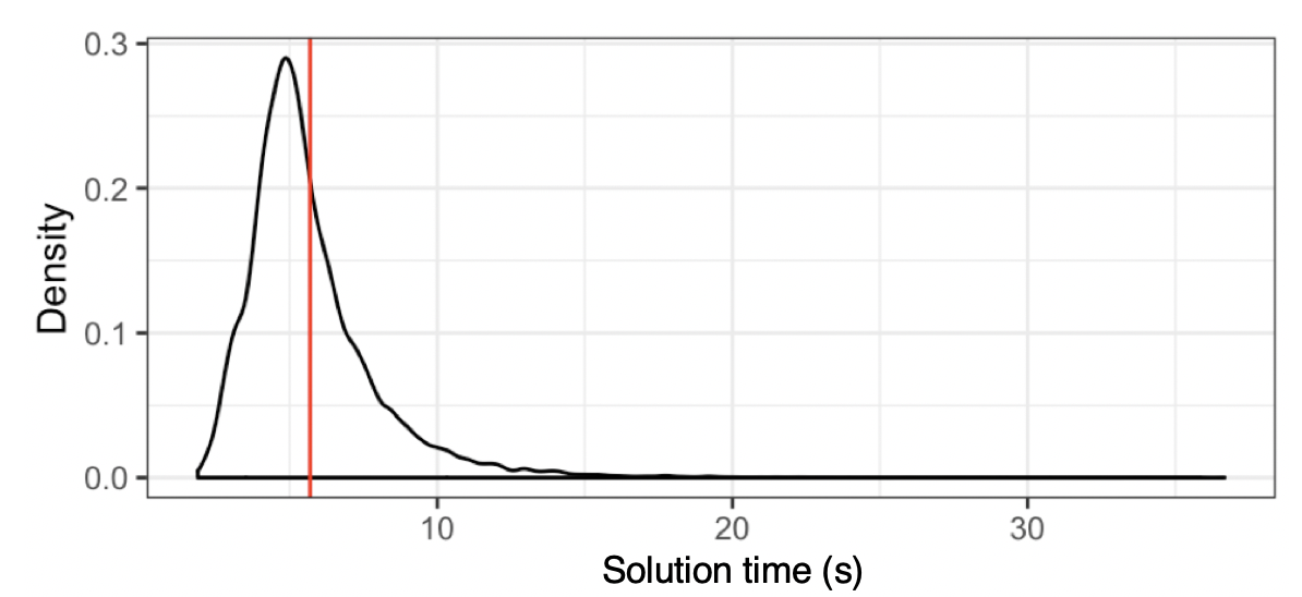
Figure 8: Distribution of 31,553 second-stage model solution times. Mean solution time $=5.7$s.

Figure 9 depicts the accuracy of the SOS2 model with anchors placed at 10% intervals for the discount multiplier axis and at $1 intervals for the rest of the fare parameters. In each trial, a fare parameter combination and a search dimension were selected uniformly at random. The “true optimal” fare parameters for each trial (i.e., each combination of current solution and search direction) were computed using a brute-force approach, through exhaustive enumeration of every solution along that affine line at a 1% granularity for discount multiplier and a $0.10 granularity for the other four fare parameters. Then the $W$ obtained through $SOS2^{*}$ procedure was evaluated and compared with this “true optimal” solution, to compute the SOS2 optimality gap. The mean optimality gap was 0.25%, and it was 0% in 29.8% of the instances. This establishes the trustworthiness of the SOS2 model outputs, especially given the drastic CPU time reduction they provide. We repeated this procedure for 10 hours, resulting in 927 solutions.

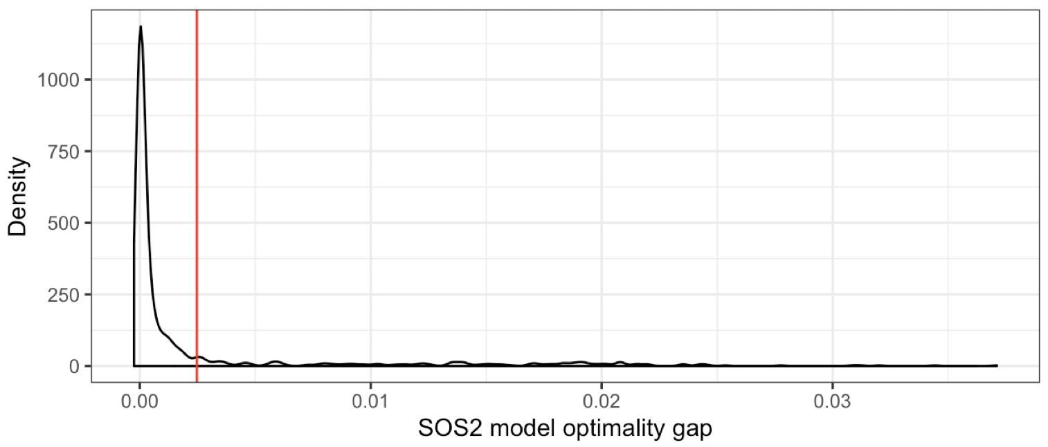
Figure 9: Distribution of SOS2 model optimality gaps. Mean gap $=0.25$%, across 927 solutions. Exact solutions (with 0% gaps) obtained in 276 of the 927 cases.

Figure 10 shows the distribution of BF-CD solution times for a single trajectory across 50 trials. BF-CD never terminates before an hour elapses.

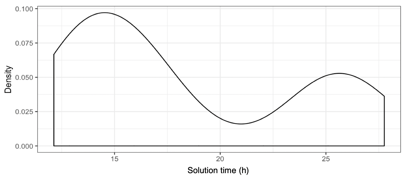
Figure 10: BF-CD single-trajectory solution times across 50 trials.

12 Bayesian Optimization Benchmark

Bayesian Optimization (BO) is a sequential search strategy for optimizing low-dimensional black-box functions (Mockus 2012). Typically, the function being optimized takes a long time to evaluate and has no analytical form, precluding access to gradients. We first provide a high-level overview of BO, and then we summarize the design choices that we use in this paper. In particular, we adapt the setup of a recent dedicated study by Liu et al. (2019) on using Bayesian Optimization to select MOD system service parameters subject to passenger mode choice. Interested readers are referred to Liu et al. (2019) for a more detailed description of BO in this application context. Readers interested in a general BO tutorial are referred to Brochu, Cora, and de Freitas (2010).

In the absence of a closed-form representation of our black-box function $f:\bm{x}\to\mathbbm{R}$, the BO framework first imposes a prior belief upon $f$ via a probabilistic surrogate model. Given this surrogate model, BO iteratively (i) updates the likelihood of historical observations with new evaluations of $f$ to obtain a more informative posterior, and (ii) queries an acquisition function that uses the updated posterior to recommend the next value of $\bm{x}$ that should be evaluated. A very common surrogate model for the black-box function is called a Gaussian Process (GP), which is a stochastic process in which any finite set of random variables follows a multivariate Gaussian distribution (Mockus 2012). After building the GP with historical observations, the GP maps a given point in the search space to a univariate Gaussian distribution. We interpret this output distribution as a set of potential values of $f(\bm{x})$, accounting for noise. The acquisition function is a BO design choice intended to help in navigating the trade-off between exploration and exploitation, i.e. exploring more of the search space versus exploiting regions where a globally optimal solution is suspected to exist. As in Liu et al. (2019), we use a GP upper confidence bound as our acquisition function, which characterizes the BO optimization process as a multi-armed bandit problem.

13 Greater Boston Area Case Study

First we describe the primary case study. Then we explain the income-aware modification to the choice model.

Primary case study.

Our case study is based on several datasets describing travel characteristics in the Greater Boston Area. We consider a pricing alliance for the morning commute, restricting our time window to 6-10AM on a typical weekday in Fall 2018. Our data sources and their purposes are as follows:

• Massachusetts Bay Transit Authority (MBTA) Focus40 report: We consider MBTA “urban gateways,” characterized as regions located beyond the rapid transit network but in close proximity to the commuter rail network. More formally, an urban gateway is a town with high potential to be receptive to additional development of public transportation options, especially if they connect to commuter rail hubs (MDOT 2019). These towns define the service region of our case study.

• MBTA Fall 2018 General Transit Feed Specification (GTFS): We use the MBTA GTFS to extract rapid transit and commuter rail stations and edges. We also collect valid transfer edges from those enumerated by the feed (MBTA 2018).

• 2017 Longitudinal Employer-Household Dynamics (LEHD) Origin-Destination Employment Statistics (LODES): This data specifies the number of jobs corresponding to each origin-destination census tract pair, where the origin represents the employee’s home tract and the destination represents their work tract. We used this data as a proxy for daily morning commute demand (U.S. Census Bureau 2017).

• U.S. Census Bureau American Community Survey, 2014-2018: We extracted town-level data on the modes of transportation to work, median household income, and total population for towns in selected priority places (U.S. Census Bureau 2018). This data was primarily used to calibrate the passenger utility parameters.

• TIGER/Line shapefiles: We used this data to assign network components to census tracts. We use the centroids of census tracts in priority places to define passenger origins and destinations (U.S. Census Bureau 2019).

• Uber Movement travel times: We used travel times aggregated over the 4th quarter of 2018 in the Greater Boston Area to approximate travel times of first- and last-mile edges and outside options (Uber Technologies Inc. 2020).

• Lyft fare parameters: We calculate the real-world prices of the MOD operator’s services using Lyft’s base fares, distance-based markups, and time-based markups (Lyft Inc. 2020). We also use this data to calibrate the passenger utility parameters.

• MBTA commuter rail fares: We characterize the real-world prices of the transit operator’s services using the MBTA commuter rail fares. We interpolate the base fares and distance-based markups from the discretized, zone-based fare structure together with the distances between transit stations in each zone (MBTA 2020).

We define the transit network using commuter rail and rapid transit edges. Each passenger’s origin and destination are census tract centroids from the LODES dataset. We built MOD operator network’s edges by connecting centroids to transit stations and to each other within each priority place. We filtered out unnecessary edges that corresponded to very low demand; implementing a 90% service goal enabled us to reduce the MOD operator’s edge set by 50%. We only consider those commuters who work locally (within their home priority place) or in the inner city (the dashed bounding box in Figure 3). Commuters to the inner city were assumed to walk the last leg of their trip, from their final transit station to their destination centroid. Because the rapid transit network is so well connected within the inner city, approximately 90% of all inner city destinations in the data were within a 0.5 mile walk of at least one transit station.

To generate the route choice sets, we first built a routing network. This routing network is a transformation of the physical network, consisting of MOD, transit, waiting, walking, and transfer edges. The cost of each edge was the time to “traverse”, whether that traversal entailed travel on the transit and/or MOD system, travel by foot, or stationary waiting. We filtered out the trips with more than one transfer, by performing a transformation on the relevant transit stations by replicating those nodes—each transfer station had one node for incoming transfers and one for outgoing transfers. A path through this network from a passenger’s origin to destination captures their total travel time along that path. Over this routing network, we implemented Yen’s algorithm for finding the $k$-shortest loopless paths over a directed graph with non-negative edge costs (Yen 1970). We first obtained up to 10 shortest paths for each commuter to the inner city. Some paths were effectively duplicates, in that every aspect of the path was the same except for the final transit station. We identified “unique” routes by their starting and transfer locations. With this definition of uniqueness, we selected the shortest path for each mode: direct via transit (with a potential walking, driving, or local bus option for the first mile, selecting whichever was the least costly from each passenger’s available options), direct via MOD operator, or hybrid (MOD first mile transferring to transit, and potentially an MOD last mile for local commuters).

We selected a route choice model specification representative of the factors influencing passenger decisions in our model: monetary costs (i.e., fares) and travel time (both within and outside the system), and alternative-specific constants (ASC) for each represented mode (driving, transit, MOD, and hybrid). To calibrate choice model parameters, we used a simplified version of the non-cooperative pricing game. We fixed fare parameters to their real-world values and selected model coefficients that make real-world fares correspond to a Nash equilibrium. This simplified game for the calibration purposes included only three passenger types: local commuters, commuters to inner city, and those traveling on the transit network outside of the alliance region. Each passenger had a simplified choice set representing average-case travel times and distances. We solved the simplified game by enumerating solutions over a coarse grid of candidate choice model coefficients values. Finally, all passengers were grouped into 3 sensitivity profiles: time-sensitive, price sensitive, and intermediate. Intermediate category uses the calibrated parameters as is. We characterize the time-sensitive passengers by doubling the time-sensitivity coefficients and halving the price-sensitivity coefficients; and vice versa for the price-sensitive passengers. Table 10 shows the final calibrated route choice model coefficients. All signs and relative magnitudes are as expected intuitively, with ASCs indicating that all else equal, people prefer driving the most and transit the least. Price and travel time impact passenger utility negatively. The calibrated parameters thus clearly pass the common sense test.

Table 10: Route choice model’s calibrated coefficients.

MOD ASC	Transit ASC	Hybrid ASC	Driving ASC	Price (USD)	Travel time (min)
-0.75	-1.125	-0.9375	0	-0.05	-0.0075

Modifications to Make the Model Income-aware.

In the modified case study in Section (5.3), rather than uniformly dividing the Greater Boston Area population into the three sensitivity profiles, we normalized time sensitivity and calibrated price sensitivity to the relative median household income (HHI) of each town, as described in Section 5.3. The price-sensitivity coefficient for each town was obtained by dividing the primary case study’s coefficient in Table 10 by that town’s income ratio. This scaling method leads to the towns with the lower values of median HHI (i.e., the towns with a lower income ratio) appropriately correspond to higher price sensitivity values.

For each town, Table 11 displays its price sensitivity coefficient and income ratio—i.e., a ratio of that town’s median HHI to the average of the median HHIs across the service region (which was $92,618.17). Absolute values of the median HHIs by town are available in Table 8. Note that the average of the median HHIs for the rest of the transit service population outside of the alliance service region is 9% higher than that within the service region, underlining that the proposed alliance particularly aims to serve lower income populations.

Table 11: Price sensitivity coefficients in the passengers’ route choice model and the income ratios by town for the income-aware case study.

Town	Price Sensitivity Coefficient	Income Ratio
Outside	-0.04592	1.0888
Brockton	-0.0840	0.5953
Framingham	-0.0585	0.8544
Waltham	-0.0541	0.9251
Lynn	-0.0848	0.5895
Salem	-0.0706	0.7079
Lowell	-0.0891	0.5613
Lawrence	-0.1114	0.4490
Haverhill	-0.0685	0.7297
Burlington	-0.0439	1.1385
Reading	-0.0411	1.2161
Wakefield	-0.0486	1.0290
Stoneham	-0.0488	1.0239
Melrose	-0.0446	1.1201
Woburn	-0.0522	0.9582
Winchester	-0.0293	1.7225

References

- Agussurja, Cheng, and Lau (2019) Agussurja L, Cheng SF, Lau HC, 2019 A state aggregation approach for stochastic multiperiod last-mile ride-sharing problems. Transp. Sci. 53(1):148–166.
- Algaba et al. (2019) Algaba E, Fragnelli V, Llorca N, Sánchez-Soriano J, 2019 Horizontal cooperation in a multimodal public transport system: The profit allocation problem. Eur. J. Oper. Res. 275.
- Banerjee et al. (2021) Banerjee S, Hssaine C, Luo Q, Samaranayake S, 2021 Plan your system and price for free: Fast algorithms for multimodal transit operations. SSRN Available at https://ssrn.com/abstract=3972423.
- Bertsimas, Ng, and Yan (2020) Bertsimas D, Ng YS, Yan J, 2020 Joint frequency-setting and pricing optimization for multi-modal transit networks at scale. Transp. Sci. 54(3):839–853.
- Bian and Liu (2019a) Bian Z, Liu X, 2019a Mechanism design for first-mile ridesharing based on personalized requirements part I: Theoretical analysis in generalized scenarios. Transp. Res. B 120:147–171.
- Bian and Liu (2019b) Bian Z, Liu X, 2019b Mechanism design for first-mile ridesharing based on personalized requirements part II: Solution algorithm for large-scale problems. Transp. Res. B 120:172–192.
- BRIDJ (2023) BRIDJ, 2023 Move Better. Acc. 4 Jan 2023 at https://www.bridj.com/#Platform.
- BRMPO (2012) BRMPO CTPS, 2012 MBTA commuter rail passenger count memorandum. Acc. 15 Sep 2022 at https://www.ctps.org/data/html/studies/transit/2012_MBTA_Commuter_Rail_Passenger_Counts/MBTA_Commuter_Rail_Passenger_Count_Results.html.
- Brochu, Cora, and de Freitas (2010) Brochu E, Cora VM, de Freitas N, 2010 A tutorial on Bayesian optimization of expensive cost functions, with application to active user modeling and hierarchical reinforcement learning. arXiv URL http://dx.doi.org/10.48550/ARXIV.1012.2599.
- Cadarso et al. (2017) Cadarso L, Vaze V, Barnhart C, Marínd A, 2017 Integrated airline scheduling: Considering competition effects and the entry of the high speed rail. Transp. Sci. 51(1):132–154.
- Castillo, Knoepfle, and Weyl (2017) Castillo JC, Knoepfle D, Weyl G, 2017 Surge pricing solves the wild goose chase. ACM Trans. Econ. Comput. 1(1).
- Chandra and Quadrifoglio (2013) Chandra S, Quadrifoglio L, 2013 A model for estimating the optimal cycle length of demand responsive feeder transit services. Transp. Res. B 51:1–16.
- Chen and Wang (2018) Chen Y, Wang H, 2018 Pricing for a last-mile transportation system. Transp. Res. B 107:57–69.
- Chun, Kleywegt, and Shapiro (2017) Chun SY, Kleywegt A, Shapiro A, 2017 When friends become competitors: The design of resource exchange alliances. Manag. Sci. 63(7):2127–2145.
- City of Jersey City, NJ (2021) City of Jersey City, NJ, 2021 Jersey City and Via launch first on-demand public bus service in New Jersey. Acc. 27 Oct 2021 at https://jerseycitynj.gov/cms/one.aspx.
- City of Newton, MA (2021) City of Newton, MA, 2021 NewMo. Acc. 5 Oct 2021 at https://www.newtonma.gov/government/planning/transportation-planning/newmo.
- City of Seattle, WA (2021) City of Seattle, WA, 2021 Via to Transit - Metro - King County. Acc. 27 Oct 2021 at https://kingcounty.gov/depts/transportation/metro/travel-options/on-demand/via-to-transit.aspx.
- Cruijssen, Dullaert, and Fleuren (2007) Cruijssen F, Dullaert W, Fleuren H, 2007 Horizontal cooperation in transport and logistics: a literature review. Transp. J. 46(3):22–39.
- Daganzo (2012) Daganzo C, 2012 On the design of public infrastructure systems with elastic demand. Transp. Res. B 46:1288–1293.
- Dallas Area Rapid Transit (2020) Dallas Area Rapid Transit, 2020 Golink: Personalized, on-demand, curb-to-curb service when and where you need it – plano zones. Acc. 1 Oct 2020 at https://www.dart.org/riding/golinkplano.asp.
- Dunning, Huchette, and Lubin (2017) Dunning I, Huchette J, Lubin M, 2017 JuMP: A modeling language for mathematical optimization. SIAM review 59(2):295–320.
- Federal Transp. Administration (2016) Federal Transp Administration, 2016 Fiscal year 2016 mobility on demand (mod) sandbox program projects. Acc. 19 Nov 2020 at https://www.transit.dot.gov/research-innovation/fiscal-year-2016-mobility-demand-mod-sandbox-program-projects.
- Fudenberg and Tirole (1991) Fudenberg D, Tirole J, 1991 Game Theory (Cambridge, MA: MIT Press).
- Gallego, Ratliff, and Shebalov (2015) Gallego G, Ratliff R, Shebalov S, 2015 A general attraction model and sales-based linear program for network revenue management under customer choice. Oper. Res. 63(1):212–232.
- Gehrke and Reardon (2018) Gehrke SR, Reardon T, 2018 Share of choices: Further evidence of the ride-hailing effect in Metro Boston and Massachusetts. Technical report, Metropolitan Area Planning Council.
- Guajardo and Rönnqvist (2016) Guajardo M, Rönnqvist M, 2016 A review on cost allocation methods in collaborative transportation. Intl. Trans. Oper. Res. 23(3):371–392.
- Hicks (2017) Hicks R, 2017 Technical memorandum: Fall 2016 monitoring of MBTA bus performance measures. Technical report, MBTA, acc. 4 Jan 2023 at https://www.ctps.org/data/calendar/htmls/2017/CMP_1221_Fall_2016_MBTA_Bus_Performance_Measures_Memo.html.
- Ho et al. (2018) Ho S, Szeto W, Kuo YH, Leung J, Petering M, Tou T, 2018 A survey of dial-a-ride problems: Literature review and recent developments. Transp. Res. B 111:395–421.
- Hu, Caldentey, and Vulcano (2013) Hu X, Caldentey R, Vulcano G, 2013 Revenue sharing in airline alliances. Manag. Sci. 59(5).
- Indianapolis Public Transp. Corporation (2021) Indianapolis Public Transp Corporation, 2021 Rides for Essential Workers. Acc. 27 Oct 2021 at https://www.indygo.net/rides-for-essential-workers/.
- Kane, Tomer, and Puentes (2016) Kane JW, Tomer A, Puentes R, 2016 How Lyft and Uber can improve transit agency budgets. Technical report, The Brookings Institution.
- Kim, Levy, and Schonfeld (2019) Kim M, Levy J, Schonfeld P, 2019 Optimal zone sizes and headways for flexible-route bus services. Transp. Res. B 130:67–81.
- Kim and Schonfeld (2014) Kim M, Schonfeld P, 2014 Integration of conventional and flexible bus services with timed transfers. Transp. Res. B 68:76–97.
- Lee and Savelsbergh (2017) Lee A, Savelsbergh M, 2017 An extended demand responsive connector. EURO J. Transp. Logist. 6:25–50.
- Li and Quadrifoglio (2010) Li X, Quadrifoglio L, 2010 Feeder transit services: Choosing between fixed and demand responsive policy. Transp. Res. C 18:770–780.
- Liu and Chow (2022) Liu Q, Chow J, 2022 Efficient and stable data-sharing in a public transit oligopoly as a coopetitive game. Transp. Res. B 163:64–87.
- Liu et al. (2019) Liu Y, Bansal P, Daziano R, Samaranayake S, 2019 A framework to integrate mode choice in the design of mobility-on-demand systems. Transp. Res. C 105:648 – 665.
- Lo, Yip, and Wan (2004) Lo HK, Yip CW, Wan QK, 2004 Modeling competitive multi-modaltransit services: A nested logit approach. Transp. Res. C 12(3-4):251–272.
- Lu, Quadrifoglio, and Petrelli (2017) Lu W, Quadrifoglio L, Petrelli M, 2017 Reliability analysis of centralized versus decentralized zoning strategies for paratransit services. Transp. Res. Proc. 25.
- Lu, Shen, and Quadrifoglio (2014) Lu W, Shen CW, Quadrifoglio L, 2014 Innovative operating strategies for paratransit services with zoning. Transp. Res. Rec. 2469.
- Lyft Inc. (2020) Lyft Inc, 2020 Boston area pricing. Acc. 14 Oct 2020 at https://www.lyft.com/pricing/bos.
- Mag (2021) Mag MT, 2021 King County Transit increases mobility options with expanded Via to Transit. https://www.masstransitmag.com/alt-mobility/shared-mobility/car-sharing, acc. 28 Mar 2022.
- MARTA (2021) MARTA, 2021 MARTAConnect. Acc. 27 Oct 2021 at https://www.itsmarta.com/marta-connect2.aspx.
- MBTA (2018) MBTA, 2018 General transit feed specification. Acc. 16 Sep 2020 at https://cdn.mbtace.com/archive/20181128.zip.
- MBTA (2020) MBTA, 2020 Commuter rail fare zones. Acc. 14 Oct 2020 at https://www.mbta.com/fares/.
- MBTA (2021) MBTA, 2021 The RIDE Flex. Acc. 26 Aug 2021 at https://www.mbta.com/accessibility/the-ride/.
- MBTA (2022) MBTA, 2022 MBTA monthly ridership by mode. Acc. 15 Sep 2022 at https://mbta-massdot.opendata.arcgis.com/datasets/MassDOT::mbta-monthly-ridership-by-mode.
- McFadden (1974) McFadden D, 1974 The measurement of urban travel demand. J. Public Econ. 3:303–328.
- MDOT (2019) MDOT, 2019 FOCUS40: the 2040 investment plan for the MBTA. Technical report, MDOT.
- MDPU (2018) MDPU, 2018 Rideshare in Massachusetts: 2018 data report. Acc. 15 Sep 2022 at https://tnc.sites.digital.mass.gov/2018/.
- Misener and Floudas (2010) Misener R, Floudas C, 2010 Piecewise-linear approximations of multidimensional functions. J. Optim. Theory Appl. 145.
- Mockus (2012) Mockus J, 2012 Bayesian Approach to Global Optimization: Theory and Applications. Mathematics and its Applications (Springer Netherlands), ISBN 9789400909090.
- Molenbruch, Braekers, and Caris (2017) Molenbruch Y, Braekers K, Caris A, 2017 Typology and literature review for dial-a-ride problems. Ann. Oper. Res. 259:295–325.
- Posada, Andersson, and Hall (2017) Posada M, Andersson H, Hall C, 2017 The integrated dial-a-ride problem with timetabled fixed route service. Public Transp. 9:217–241.
- Rasulkhani and Chow (2019) Rasulkhani S, Chow J, 2019 Route-cost-assignment with joint user and operator behavior as a many-to-one stable matching assignment game. Transp. Res. B 124:60–81.
- Regional Transp. Commission of Southern Nevada (2021) Regional Transp Commission of Southern Nevada, 2021 RTC On-Demand Pilot Program. Acc. 26 Aug 2021 at https://www.rtcsnv.com/ways-to-travel/paratransit-accessibility/.
- Schaller (2018) Schaller B, 2018 The new automobility: Lyft, Uber and the future of american cities. Technical report, Schaller Cons.
- Schlicher and Lurkin (2022) Schlicher L, Lurkin V, 2022 Stable allocations for choice-based collaborative price setting. Eur. J. Oper. Res. 302(3).
- Schrank et al. (2015) Schrank D, Eisele B, Lomax T, Bak J, 2015 Urban mobility scorecard. Technical report.
- Siddiq, Tang, and Zhang (2021) Siddiq A, Tang CS, Zhang J, 2021 Partnerships in urban mobility: Incentive mechanisms for improving public transit adoption. Manuf. Serv. Oper. Manag. Articles in Advance.
- St. Louis Metro (2021) St Louis Metro, 2021 $1 Lyft trips to transit connections. Acc. 27 Oct 2021 at https://www.metrostlouis.org/lyft/.
- Stiglic et al. (2018) Stiglic M, Agatz N, Savelsbergh M, Gradisar M, 2018 Enhancing urban mobility: Integrating ride-sharing and public transit. Comput. Oper. Res. 90:12–21.
- The Boston Globe (2022) The Boston Globe, 2022 With NewMo, Newton’s rideshare service continues to grow. https://www.bostonglobe.com/2022/02/16/metro/with-newmo-newtons-rideshare-service-continues-grow/, acc. 28 Mar 2022.
- The Economist (2018) The Economist, 2018 Public transport is in decline in many wealthy cities. www.economist.com/international/2018/06/21/public-transport-is-in-decline-in-many-wealthy-cities.
- Uber Technologies Inc. (2020) Uber Technologies Inc, 2020 Uber movement. Acc. 16 Sep 2020 at https://movement.uber.com.
- U.S. Census Bureau (2017) US Census Bureau, 2017 Longitudinal employer-household dynamics origin-destination employment statistics. Acc. 16 Sep 2020 at https://lehd.ces.census.gov/data/.
- U.S. Census Bureau (2018) US Census Bureau, 2018 Census reporter. Acc. 28 Sep 2020 at https://censusreporter.org/tables/.
- U.S. Census Bureau (2019) US Census Bureau, 2019 TIGER/Line shapefiles. Acc. 21 Sep 2020 at https://www2.census.gov/geo/tiger/TIGER2019/TRACT/.
- Via Transp. (2023) Via Transp, 2023 The Backbone of a Modern Transportation System. Acc. 4 Jan 2023 at https://ridewithvia.com/solutions.
- Wang (2019) Wang H, 2019 Routing and scheduling for a last-mile transportation system. Transp. Sci. 53(1):131–147.
- Wang, Jacquillat, and Vaze (2022) Wang K, Jacquillat A, Vaze V, 2022 Vertiport planning for urban aerial mobility: An adaptive discretization approach. Manuf. Serv. Oper. Manag. 24(6):3215–3235.
- Wang, Agatz, and Erera (2018) Wang X, Agatz N, Erera A, 2018 Stable matching for dynamic ride-sharing systems. Transp. Sci. 52(4):850–867.
- Wei, Vaze, and Jacquillat (2020) Wei K, Vaze V, Jacquillat A, 2020 Airline timetable development and fleet assignment incorporating passenger choice. Transp. Sci. 54(1):139–163.
- Williams (1977) Williams H, 1977 On the formation of travel demand modelsand economic evaluation measures of user benefit. Environ. Plan. A 9(3):285–344.
- Wright, Groenevelt, and Shumsky (2010) Wright CP, Groenevelt H, Shumsky RA, 2010 Dynamic revenue management in airline alliances. Transp. Sci. 44(1).
- Yen (1970) Yen J, 1970 An algorithm for finding shortest routes from all source nodes to a given destination in general networks. Q. Appl. Math. 27.