On Advantages of Mask-level Recognition for Outlier-aware Segmentation

Abstract

Most dense recognition approaches bring a separate decision in each particular pixel. These approaches deliver competitive performance in usual closed-set setups. However, important applications in the wild typically require strong performance in presence of outliers. We show that this demanding setup greatly benefit from mask-level predictions, even in the case of non-finetuned baseline models. Moreover, we propose an alternative formulation of dense recognition uncertainty that effectively reduces false positive responses at semantic borders. The proposed formulation produces a further improvement over a very strong baseline and sets the new state of the art in outlier-aware semantic segmentation with and without training on negative data. Our contributions also lead to performance improvement in a recent panoptic setup. In-depth experiments confirm that our approach succeeds due to implicit aggregation of pixel-level cues into mask-level predictions.

1 Introduction

Emergence of deep learning revolutionized the field of computer vision [34]. Complex yet efficient deep networks advanced the capability of machines to understand scenes [20, 61]. Segmentation is a very important form of scene understanding due to its applications in medicine, agriculture, robotics and the automotive industry. In the last decade, segmentation tasks were modelled as per-pixel classification [20, 44]. However, such approach assumes independence of neighbouring pixels, which does not hold in practice. Neighbouring pixels are usually strongly correlated due to belonging to the same object or scene part [39]. Albeit designed and trained with false assumption on independence of neighbouring pixels, the obtained models deliver competitive generalization performance in in-distribution scenes [14, 15]. However, their real-world performance still leaves much to be desired due to insufficient handling of the out-of-taxonomy scene parts [6, 11].

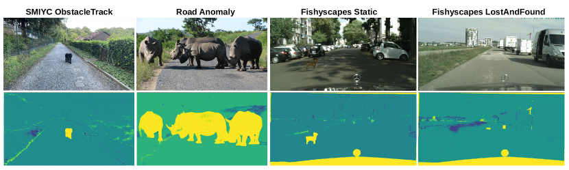
Figure 1: Outlier-aware segmentation with the proposed mask-level approach. We present input images (top) and dense OOD scores (bottom).

A recent approach to per-pixel classification decouples localization from recognition [17]. The localization is carried out by assigning pixels to an abundant set of masks, each trained to capture semantically related regions (e.g. a road or a building). The recovered semantic regions are subsequently classified as a whole. The described approach is dubbed mask-level recognition [16]. Decoupling localization from classification further enables utilizing the same model for semantic, instance and panoptic segmentation. The shared architecture performs competitively on standard segmentation benchmarks [39, 18, 64].

However, prior work does not consider demanding applications of mask-based approaches. Thus, we investigate the value of mask-level recognition in some of the last major remaining challenges towards scene understanding in the wild - outlier-aware semantic segmentation [7, 11, 29] and outlier-aware panoptic segmentation [29]. Our experiments reveal strong performance of mask-level approaches in these challenges. We investigate the reasons behind such behaviour and contribute improvements that support these important applications.

Mask-level recognition has several interesting properties. For instance, masks are classified into K known classes and the class void, while mask assignments are not mutually exclusive [17]. This provides more opportunity to reject predictions than in standard per-pixel approaches. Mask-level approaches can propagate mask-level uncertainty to the pixel-level. This is different from the standard approach which has to estimate independent anomaly scores in each pixel [26]. Obviously, the standard approach can easily ignore the local correlations in a pixel neighborhood, which does not seem desirable. In terms of scalability, mask-level recognition models do not require per-class feature maps at the output resolution. This allows designers to decrease the training footprint [8] and increase the flexibility of training. All these properties make mask-level recognition a compelling research topic.

This paper proposes the following contributions. We point out that mask-level recognition delivers strong baseline performance on standard benchmarks for outlier-aware segmentation. Our improvements further exploit the specific bias of mask-level recognition. Combining the proposed EAM outlier detector with negative supervision attains competitive results in outlier-aware semantic and panoptic segmentation. Further improvements can be obtained by combining the proposed approach with negative supervision. The resulting models set the new state of the art in outlier-aware segmentation on two tracks from the Segment Me If You Can (SMIYC) benchmark and adapted MS COCO.

2 Related work

The related work considers models for mask-level recognition tasks (Sec. 2.1) and segmentation in presence of outliers (Sec. 2.2).

2.1 Recognition of free-form regions

Early approaches to mask-wide recognition relied on class-agnostic bottom-up proposals. They aggregated hand-crafted [9] or convolutional [25, 19, 51] features along the proposed regions and brought mask-wide decisions by classifying pooled representations. Mask-RCNN extends this approach by sharing features across detection of proposals and mask-wide classification, as well as by end-to-end training of all parameters. Recently, PointRend proposes to back-propagate the loss only through selected low-uncertainty predictions [33]. This allows to increase mask-RCNN resolution from 28$\times$28 to 224$\times$224 with a neglectable impact on the training footprint. Very recently, MaskFormer precludes dependence on bottom-up proposals by directly assigning pixels to masks that span arbitrary image regions [17]. Its key component is a hypernetwork [24] that produces the weights for two 1$\times$1 convolutions that convert pixel-level embeddings into mask assignment scores and, subsequently, into semantic maps. This is the first architecture that succeeds to deliver competitive experimental performance on three dense recognition tasks: semantic segmentation, instance segmentation, and panoptic segmentation. Mask2Former [16] further improves the mask hypernetwork by introducing a special kind of attention layer that promotes progressive focusing onto foreground pixels for a particular mask. Our work explores the Mask2Former performance in the context of outlier-aware segmentation and outlier-aware panoptic segmentation.

2.2 Segmentation in presence of outliers

Recognition in the wild involves test regions beyond the training taxonomy. Adequate models should reject the decision in such pixels [54]. This can be carried out by restricting the shape of the decision boundary [55, 1] or by complementing the classifier with an anomaly detector [27, 38]. The decision boundary can be restricted by thresholding distance from the learned class centers in the embedding space [55, 10]. This can be further improved by employing a stronger classifier [58]. Nevertheless, many of these approaches are bound to fail if unknown samples happen to map to the same features as the samples from the known classes. This occurrence is known as feature collapse [45].

Early approaches for extending discriminative predictions with OOD detection have been based on prediction confidence [27], input perturbations [38], density estimation [48] and Bayesian uncertainty [47]. Several studies point out that semantic anomalies [53] may be especially hard to detect [48, 56, 32]. A promising approach involves generating synthetic anomalies in tandem with the discriminative task [35, 63, 22, 13]. Further empirical improvements have been achieved by mimicking anomalies with negative training data [28, 42]. However, this may lead to over-optimistic performance estimates due to possible overlap with test anomalies.

Outlier detection is especially interesting in the dense prediction context due to important applications in robust scene understanding [7, 11, 62]. However, straight-forward adaptations of image-wide approaches experience two important failure modes. First, they often fail to accurately localize anomalies in front of inlier backgrounds [3]. Second, they are prone to false positives in inlier pixels with high entropy predictions that occur regularly at semantic borders [52]. Hence, a large body of work proposes custom designs to alleviate these problems.

Partially anomalous images can be accounted for by learning on mixed-content images [3, 23, 5, 57]. Correlation between neighbouring pixels can be addressed by aggregating evidence through meta-classification [52] or input pre-processing [38]. Real training data can be avoided by fitting generative heads to pre-trained [7] or jointly trained [29, 37] features. Another line of work trains on synthetic negatives corresponding to adversarial noise [2] or samples of a jointly trained generative model [21]. Finally, some approaches detect the discrepancy between the input and the resynthesised scene [41, 60, 5, 59].

Different than all previous works, we formulate outlier detection according to mask-wide predictions. Different than meta-classification approaches [52, 12] our method requires only one learning episode and does not require negative data. Our method is orthogonal to most previous approaches and it, therefore, represents an exciting baseline for future work.

3 Mask-level recognition in presence of outliers

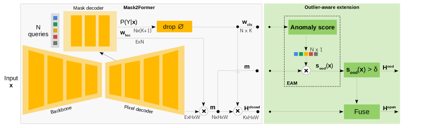
Figure 2: We focus on three tensors that are produced by the standard M2F model (left) [16]: closed-set segmentation $\mathbf{H}_{\mathrm{closed}}$ (K$\times$H$\times$W), per-mask dense binary assignments $\mathbf{m}$ (N$\times$H$\times$W), and image-wide mask-level class scores $\mathbf{w}_{\mathrm{cls}}$ (N$\times$K). We start our outlier-aware extension (right) by quantifying uncertainty of mask-level predictions $\mathbf{w}_{\mathrm{cls}}$. We recover the dense anomaly map $\mathbf{s}_{\mathrm{OOD}}^{\mathrm{EAM}}$ (H$\times$W) by redistributing per-mask anomaly scores back to the pixels according to dense mask assignment $\mathbf{m}$ as shown in (7). We assemble outlier-aware segmentation $\mathbf{H}_{\mathrm{open}}$ by thresholding $\mathbf{s}_{\mathrm{OOD}}^{\mathrm{EAM}}$ and fusing it with $\mathbf{H}_{\mathrm{closed}}$. Note that $\sum_{rc}\mathbf{m}_{i}[r,c]\neq 1$.

We present a novel approach for extending mask-level dense prediction towards outlier-aware segmentation. Our approach can operate above many of the recent dense prediction approaches based on mask-level recognition [29, 17, 36]. We formulate a novel dense OOD score by ensembling mask-wide anomaly scores. This improves outlier-aware segmentation on real datasets due to aggregating pixel-level evidence across image regions and decreasing sensitivity to semantic boundaries.

3.1 Semantic segmentation with mask-level recognition

Mask-level segmentation approaches decouple classification from localization and model them with separate prediction heads [17]. Localization can be formulated through probabilistic assignments (masks) $\mathcal{S}=\{\mathbf{m}_{i}\,|\,i=1,\dots,N\}$ that capture semantically related regions. Each mask $\mathbf{m}_{i}$ is an $H\times W$ array of probabilistic assignments to the corresponding pixel. We can join masks into 3D tensor $\mathbf{m}^{N\times H\times W}$. Masks are recovered by subjecting standard dense features $\mathbf{E}$ to inferred projection $\mathbf{w}_{\mathrm{loc}}$ and sigmoid activation:

$$\mathbf{m}=\sigma(\mathrm{conv}_{1\times 1}(\mathbf{E},\mathbf{w}_{\mathrm{loc}})).$$ (1)

Recognition can be carried out by inferring N mask-wide categorical distributions into K known classes and one void class. We denote these predictions as $P_{i}(Y=k|\mathbf{x})$, $i\in$ 1..N, $k\in$ 1..K+1. Let us consider probabilities of non-void classes and arrange them into a $N\times K$ matrix $\mathbf{w}_{\mathrm{cls}}$. Then the tensor of closed-set semantic segmentation scores can be recovered by projecting masks according to $\mathbf{w}_{\mathrm{cls}}$:

$$\mathbf{H}_{\mathrm{closed}}=\mathrm{conv}_{1\times 1}(\mathbf{m},\mathbf{w}_{\mathrm{cls}}).$$ (2)

Note that this tensor does not contain distributions since $\sum_{i}m_{i}[r,c]\neq 1$ and $\sum_{k}\mathbf{w}_{\mathrm{cls}}[i,k]\neq 1$. The above convolution can be interpreted as classifying each pixel (r,c) according to a weighted ensemble of per-mask classifiers where the weights correspond to dense mask assignments:

$$\hat{y}[r,c]=\underset{k=1\dots K}{\mathrm{argmax}}\sum_{i}\mathbf{m}_{i}[r,c]\cdot P_{i}(Y=k|\mathbf{x})\;.$$ (3)

Figure 2 (left) shows that dense features $\mathbf{E}$ are produced in usual fashion, by connecting an off-the-shelf backbone to an upsampling decoder with skip connections. The main novelty is a hypernetwork denoted as mask decoder that receives latent features and infers image-wide weights $\mathbf{w}_{\mathrm{loc}}$ and $\mathbf{w}_{\mathrm{cls}}$. The training fits mask assignments $\mathbf{m}$ and mask-level recognition $P_{i}(Y=k|\mathbf{x})$ to the dense labels.

3.2 Detecting outliers in pixel-level predictions

Dense OOD detection requires a scoring function $\mathbf{s}_{\mathrm{ood}}:[0,255]^{3\times H\times W}\rightarrow\mathcal{R}^{H\times W}$ that maps each pixel to the corresponding anomaly score. Subsequently, we can detect anomalies by thresholding the anomaly score $\mathbf{s}_{\mathrm{ood}}(\mathbf{x})$. We can recover outlier-aware segmentation by fusing anomalies with closed-set segmentation.

Several standard baselines detect anomalous regions according to uncertainty of pixel-level predictions [7, 26]. The prediction uncertainty can be quantified as max-score [27], entropy [12], energy [42] etc. We shall evaluate that approach by the PerPixel baseline that ablates the mask decoder and replaces it with standard per-pixel predictions [44].

Pixel-level predictions can also be recovered with a mask-level model. The training procedure encourages masks $\mathbf{m}_{i}$ to specialize for capturing specific visual concepts. Hence, one could define a pixel-level anomaly score which rejects pixels that are not claimed by any mask:

$$\mathbf{s}_{\mathrm{ood}}^{\mathrm{AM}}(\mathbf{x})[r,c]=-\max_{i}\mathbf{m}_{i}[r,c]$$ (4)

AM stands for Anomaly of the max-Mask. Accordingly, we shall have a high anomaly score where all masks have low confidence. Even though this approach outperforms the per-pixel baseline, it is far from perfect. Fig. 3 shows histograms of inliers and outliers on Fishyscapes L&F val according to $\max{m}_{i}$ score.

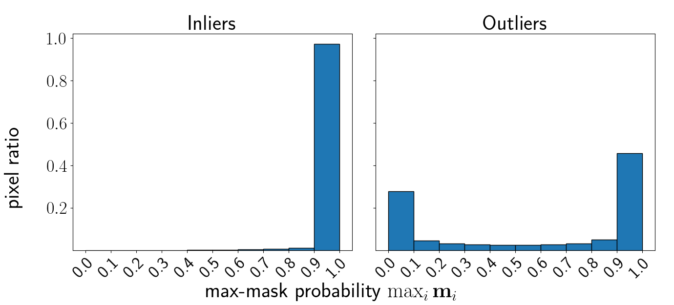
Figure 3: Relative pixel frequencies according to max mask probability in inlier and outlier pixels on Fishyscapes L&F val.

The left histogram reveals that almost all inliers have high-confidence mask assignments. On the other hand, the outlier distribution is highly polarized. The left mode can be easily distinguished from inliers, but the right mode presents a tougher challenge. This suggests that pixel-level predictions may not be an optimal solution to our problem, because many of the real outlier pixels get high confidence mask assignments. Therefore, we consider to build on mask-level uncertainty.

3.3 Detecting outliers in mask-level predictions

We first consider a method that recovers dense anomaly scores as mask-level uncertainty of the strongest mask. If we choose max-softmax as the uncertainty measure, we can formulate this score as:

$$\mathbf{s}_{\mathrm{ood}}^{\mathrm{AHM}}(\mathbf{x})[r,c]=-\!\!\max_{k=1\dots K}P_{\mathrm{argmax}_{i}\mathbf{m}_{i}[r,c]}(Y=k|\mathbf{x}).$$ (5)

AHM stands for Anomaly score of Hard-assigned Masks. However, this approach completely ignores the uncertainty of the dominant mask assignment. This clearly feels suboptimal and our empirical results confirm this intuition. Therefore, we set out to combine uncertainties of pixel-level mask assignment and mask-level recognition.

We proceed by considering closed-set semantic segmentation scores (3). We can quantify their uncertainty according to an arbitrary anomaly detector. If we choose max-logit detector [26], we obtain the following:

$$\mathbf{s}_{\mathrm{ood}}^{\mathrm{AEM}}(\mathbf{x})[r,c]=-\!\!\max_{k=1\dots K}\sum_{i}\mathbf{m}_{i}[r,c]\cdot P_{i}(Y=k|\mathbf{x}).$$ (6)

Closed-set semantic scores can be viewed as ensembled outputs of per-mask classifiers, where mask assignments act as weights of the ensemble members. Hence, we denote this score as Anomaly of Ensembled Mask-wide predictions (AEM).

Finally, we consider to apply anomaly detector directly to mask-level classification scores. We propose to aggregate the resulting evidence in each particular pixel according to its mask assignments $\mathbf{m}$. This approach can be interpreted as an Ensemble over Anomaly scores of Mask-wide predictions (EAM). This approach has an intuitive appeal due to direct relation towards mask-level uncertainty. If we quantify mask-level uncertainty according to maximum per-class probability, we get a lower bound of the AEM score (6):

$$\mathbf{s}_{\mathrm{ood}}^{\mathrm{EAM}}(\mathbf{x})[r,c]=\sum_{i}\mathbf{m}_{i}[r,c]\cdot(-\max_{k=1\dots K}P_{i}(Y=k|\mathbf{x}))\\ \leq-\max_{k=1\dots K}\sum_{i}\mathbf{m}_{i}[r,c]\cdot P_{i}(Y=k|\mathbf{x})$$ (7)

Fig. 2 (right) illustrates steps to compute the EAM score from M2F outputs.

We expect that the difference between the two approaches should be best visible at semantic borders. Here adjacent masks often lower their pixel assignment confidence. In such situations our proposed EAM approach will correctly output a lower anomaly score than AEM. Fig. 4 illustrates the differences between EAM and AEM scoring on two scenes from Fishyscapes L&F. We observe a similar behaviour in most of image pixels. However, the proposed EAM approach clearly outputs lower anomaly score on semantic boundaries. This can help by reducing false positive detections in inlier pixels at semantic boundaries.

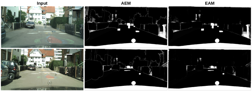
Figure 4: Pixel-level vs. mask-level OOD detection. Mask-level OOD detection alleviates the known issue of false positives at semantic borders. Please zoom in for the details.

3.4 Performance enhancement with negative data

Training with negative data is an important component of many recent outlier detection approaches [28, 5, 12, 23, 57] due to the potential to address feature collapse. In the case of dense prediction this usually involves pasting negative data over the inlier training images [3, 21]. Existing implementations require an additional loss term in negative pixels [42, 28, 12]. On the contrary, our approach does not require any changes in the model or the loss function.

We propose to set the ground truth of negative pixels to void class. This instructs all masks to steer clear of negative pixels. This is reasonable since void pixels do not belong to any class of interest. Such training increases the variety of void content and masks get penalized if they claim any.

The standard dense classifiers [14, 50] cannot be trained with negatives labeled as void. Reason for this lies in the standard per-pixel cross-entropy loss which is not computed in void pixels. Hence, our pasting procedure is specific for mask-level recognition.

Figure 5 shows a training example: the input image crop and the corresponding ground truth binary labels. None of the ground truth labels encapsulate the pasted negative pixels. Our experiments show that this kind of supervision generalizes to outlier detection in real-world images.

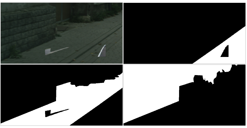
Figure 5: Mixed-content training image (top left) and mask-assignment groundtruth for classes road (top-right), sidewalk (bottom-left) and building (bottom-right). The model is trained to reject the two pasted negative instances from all masks.

4 Experiments

Our experiments explore advantages of mask-level recognition for in outlier-aware semantic segmentation. We consider semantic (Sec. 4.1) and panoptic segmentation (Sec. 4.2).

4.1 Outlier-aware segmentation of road-driving images

We evaluate outlier-aware segmentation performance on two standard benchmarks. The Fishyscapes benchmark includes two tracks that focus on urban road driving [7]. The FS L&F track relabels a subset of the Lost and Found dataset. The FS Static track pastes anomalous objects in images from Cityscapes val. The SMIYC benchmark (Segment Me If You Can) includes two tracks with real-world anomalies in very diverse environments. The Anomaly Track includes large anomalies that can occur anywhere in the image, while the Obstacle Track focuses on small anomalies on the road surface.

We measure the performance of OOD detection according to average precision (AP) and FPR at TPR of 95% ($\mathrm{FPR}_{95}$). We use Mask2Former (M2F) [16] with Swin-L [43] backbone. Following the usual conventions, we train our models in two regimes: with and without negative data. Our models without auxiliary data consider only Cityscapes images [18]. This likely reduces our performance on SMIYC due to large domain shift [58]. Models with negative data are first trained with Cityscapes taxonomy on images from Cityscapes and Mapillary Vistas [49]. Then, we fine-tune the model for 2K iterations on mixed-content images. We paste ADE20K [64] instances as negative data. We use standard hyper-parameters [16] except for the batch size, which we set to 18. The longest experiments last about 48 hours on 3$\times$A6000.

Table 1 compares the performance of our best approach (M2F-EAM) with the related work on SMIYC. The two sections organize the methods depending on whether they train on real negative data. Our model trained without negative data achieves strong average precision in both tracks. High AP and comparatively poor $\mathrm{FPR}_{95}$ scores suggest rare occurrences of highly confident false negative detections. Analysis of the AUROC curve supports this hypothesis since we achieve $\mathrm{FPR}_{90}$ = $20\%$.

Training on more diverse closed-set images and fine-tuning with negative data significantly improves the results. Moreover, our model trained with auxiliary data achieves state-of-the-art performance on SMIYC benchmark across all metrics. Dramatic improvement in FPR suggests that training with negative data improves models ability to detect diverse anomalies.

Method	Aux	AnomalyTrack		ObstacleTrack
	data	AP	$\mathrm{FPR}_{95}$	AP	$\mathrm{FPR}_{95}$
Image Resyn. [41]	✗	52.3	25.9	37.7	4.7
Road Inpaint. [40]	✗	-	-	54.1	47.1
JSRNet [59]	✗	33.6	43.9	28.1	28.9
Max softmax [27]	✗	28.0	72.1	15.7	16.6
MC Dropout [31]	✗	28.9	69.5	4.9	50.3
ODIN [38]	✗	33.1	71.7	22.1	15.3
Embed. Dens. [7]	✗	37.5	70.8	0.8	46.4
M2F-EAM (ours)	✗	76.3	93.9	66.9	17.9
SynBoost [5]	✓	56.4	61.9	71.3	3.2
DenseHybrid [23]	✓	78.0	9.8	78.7	2.1
PEBAL [57]	✓	49.1	40.8	5.0	12.7
Void Classifier [7]	✓	36.6	63.5	10.4	41.5
Maxim. Ent. [12]	✓	85.5	15.0	85.1	0.8
M2F-EAM (ours)	✓	93.8	4.1	92.9	0.5

Table 1: Outlier-aware segmentation on SMIYC. Our AP performance outperforms all previous approaches in both categories.

Table 2 compares our method (M2F-EAM) with related work on the Fishyscapes benchmark [6]. As before, the two sections gather methods based on whether they use real negative data (bottom) or not (top). Our method achieves the best performance on FS Static in both categories and the best AP performance on FS Lost and Found.

Method	FS L&F		FS Static		CS Val
	AP	$\mathrm{FPR}$	AP	$\mathrm{FPR}$	mIoU
Maxim. Ent. [12]	15.0	85.1	0.8	77.9	9.7
Image Resyn. [41]	5.7	48.1	29.6	27.1	81.4
Max softmax [27]	1.8	44.9	12.9	39.8	80.3
SML [30]	31.7	21.9	52.1	20.5	-
Embed. Dens. [7]	4.3	47.2	62.1	17.4	80.3
NFlowJS [22]	39.4	9.0	52.1	15.4	77.4
SynDHybrid [23]	51.8	11.5	54.7	15.5	79.9
M2F-EAM (ours)	9.4	41.5	76.0	10.1	83.5
SynBoost [5]	43.2	15.8	72.6	18.8	81.4
Prior Entropy [46]	34.3	47.4	31.3	84.6	70.5
OOD Head [4]	30.9	22.2	84.0	10.3	77.3
Void Classifier [7]	10.3	22.1	45.0	19.4	70.4
Dirichlet prior [46]	34.3	47.4	84.6	30.0	70.5
DenseHybrid [23]	43.9	6.2	72.3	5.5	81.0
PEBAL [57]	44.2	7.6	92.4	1.7	-
M2F-EAM (ours)	63.5	39.2	93.6	1.2	83.5

Table 2: Outlier-aware segmentation on Fishyscapes benchmark. Our AP performance outperforms all previous approaches.

Table 3 evaluates outlier-aware segmentation on validation subsets of Road Anomaly [41] and Fishyscapes [6]. We compare our mask-level approaches with the standard pixel-level baseline (PerPixel) and the previous work. Again, methods from the bottom section train on auxiliary negative data while the others see only inliers. Our two mask-level approaches outperform the pixel-level baseline and all previous approaches. Among the two mask-level approaches, ensemble over anomaly scores (M2F-EAM) outperforms anomaly score of the ensemble (M2F-AEM).

Model	Road Anomaly		FS L&F		FS Static
	AP	$\mathrm{FPR}$	AP	$\mathrm{FPR}$	AP	$\mathrm{FPR}$
MSP [27]	15.7	71.4	4.6	40.6	19.1	24.0
ML [26]	19.0	70.5	14.6	42.2	38.6	18.3
NFlowJS [21]	-	-	40.2	18.7	34.4	11.2
SML [30]	25.8	49.7	36.6	14.5	48.7	16.8
SynthCP [60]	24.9	64.7	6.5	46.0	23.2	34.0
Density [7]	-	-	4.1	22.3	-	-
PerPixel	49.3	31.0	2.5	56.7	11.5	34.8
M2F-AEM	66.9	15.3	51.2	28.0	86.2	3.5
M2F-EAM	66.7	13.4	52.0	20.5	87.3	2.1
SynBoost[5]	38.2	64.8	60.6	31.0	66.4	25.6
Energy [42]	19.5	70.2	16.1	41.8	41.7	17.8
PEBAL[57]	45.1	44.6	58.8	4.8	92.1	1.5
DenseHybrid [23]	-	-	63.8	6.1	60.0	4.9
M2F-EAM	69.4	7.7	81.5	4.2	96.0	0.3

Table 3: Comparison of our mask-level approaches (M2F-EAM, M2F-AEM) with the pixel-level baseline (PerPixel) and the previous work on RoadAnomaly and Fishyscapes val.

4.2 Outlier-aware panoptic segmentation on MS COCO

Mask-level outlier detection can also be applied for panoptic segmentation. We consider the hardest setup from a recent related work [29] that relabels 20% of thing classes from COCO as void pixels during training. These classes are dining table, banana, bicycle, cake, sink, cat, keyboard, and bear. During inference the model has to classify all pixels from these classes into the dedicated anomalous thing class. Outlier-aware performance is measured according to standard metrics PQ, SQ, and RQ. Our models use a ResNet-50 backbone as in the previous work [29].

Mask-level training encourages all masks to refrain from encompassing the void pixels. Our anomaly detectors are sensitive to the resulting lack of mask assignment. Hence, the intensity of our supervision is very similar to void-suppression [29]. Our inference recovers the dense anomaly map by thresholding the mask-level anomaly score. We validate the threshold for 95% TPR in outlier detection on a held-out validation image. We assign each anomalous pixel to its prefered mask and form instances by keeping all masks with more than 200 pixels.

Table 4 compares our method to several approaches from the EOPSN paper [29]. We outperform all previous work, in spite of much less supervision. Note that our method can easily accommodate anomalous stuff classes.

Method	Known			Unknown
	PQ	SQ	RQ	PQ	SQ	RQ
Void-background	37.7	76.3	46.6	4.0	71.1	5.7
Void-ignorance	37.2	76.3	45.9	3.7	71.8	5.2
Void-suppression	37.5	75.9	46.1	7.2	75.3	9.6
Void-train	36.9	76.4	45.5	7.8	73.4	10.7
EOPSN [29]	37.4	76.2	46.2	11.3	73.8	15.3
Open-M2F-AEM	43.5	82.0	52.2	11.3	73.3	15.3
Open-M2F-EAM	43.5	82.0	52.2	13.2	73.4	18.0

Table 4: outlier-aware panoptic segmentation on COCO. We relabel 20% of thing classes to the unknown void class [29]. We outperform other approaches both on known and unknown classes.

Figure 6 shows qualitative results on three scenes from COCO val. The rows show: input image, ground truth, two results from [29] and finally our results. The results clearly illustrate improvements of our method over previous state of the art in outlier-aware panoptic segmentation.

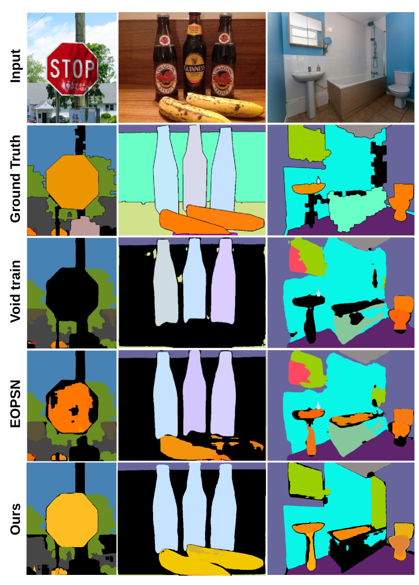
Figure 6: outlier-aware panoptics with M2F-EAM. Stop sign, bananas, toilet and sink are considered unknown thing classes [29]. We detect all unknown classes and distinguish some instances.

Note finally that panoptic mask-level models can also be used for standard outlier-aware semantic segmentation. In fact, panoptic models outperform their semantic counterparts in 3 out of 6 metrics from Table 3.

5 Ablations

We ablate the choice of the OOD score (Sec. 5.1), the backbone (Sec. 5.2), the number of masks (Sec. 5.3), and the source of negative data (sec. 5.4).

5.1 Impact of the OOD score

Table 5 considers several OOD detectors that can be plugged into our methods. The five sections consider per-pixel baseline and the aforementioned M2F-AM, M2F-AHM, M2F-AEM, and M2F-EAM. We note that neither ensembles of mask scores nor the mask scores themselves are distributions. Hence we do not consider probabilistic anomaly detectors in the last four sections. Instead, we only consider simply taking the hard maximum (this is related to max-softmax) or the energy score (log-sum-exp). The two options perform comparably so we choose to use hard maximum in our submissions to SMIYC as a simpler choice. As before, we observe slight advantage of M2F-EAM over M2F-AEM, as well as poor performance of per-pixel outlier detection that is in line with previous work [7, 26]. Additionally, we observe that ensemble-based methods outperform their simpler counterparts M2F-AM and M2F-AHM.

Method	Anomaly detector	FS L&F	FS Static
PerPixel	Entropy [28]	2.9	12.7
	KL div [22]	4.1	16.4
	Energy [42]	2.4	11.3
	Max-softmax [27]	1.8	8.9
M2F-AM	Max-score	30.9	30.2
M2F-AHM	Max-score	3.5	44.4
M2F-AEM	Energy	51.1	86.6
	Max-score	51.2	86.2
M2F-EAM	Energy	48.5	69.3
	Max-score	52.0	87.3

Table 5: Validation of anomaly detectors that can plug-in into our methods. Energy score (log-sum-exp) performs similar to taking a hard maximum. Again, M2F-EAM outperforms M2F-AEM while both mask-level approaches outperform M2F-AM, M2F-AHM, and per-pixel baseline.

5.2 Impact of the backbone

Table 6 investigates OOD detection performance of per-pixel and mask-classification models with different backbones. We consider two convolutional backbones, ResNet-50 and a more advanced ConvNeXt-L. We also consider transformer-based backbone Swin-L. Additionally, we show results of DeepLabV3+ model with ResNet-50 backbone. Our per-pixel baseline and DLv3+ perform similarly while Mask2Former outperforms both methods. Strong performance of M2F models based on Swin-L suggests that large capacity and transformer architecture may be important for mask-based outlier-aware segmentation.

Backbone	Model	FS L&F		FS Static		CS val
		AP	$\mathrm{FPR}$	AP	$\mathrm{FPR}$	mIoU
ResNet-50	DLv3+	3.5	45.0	-	-	77.8
	PerPixel	1.3	64.0	9.0	42.9	79.6
	M2F-EAM	20.8	22.7	36.7	23.8	79.4
ConvNeXt-L	M2F-EAM	31.5	28.6	76.3	6.3	82.6
Swin-L	PerPixel	2.5	56.7	11.5	34.8	83.2
	M2F-EAM	52.0	20.5	87.3	2.1	83.5

Table 6: Comparison of several models with different backbones on Fishyscapes val. Mask-level models outperform their per-pixel counterparts, and this is a major takeaway of our work.

5.3 Impact of the mask count

Table 7 explores the significance of the number of masks N for closed-set recognition and outlier detection. We consider the case where the number of masks equals the number of classes (N=19) as well as two more abundant choices (N=50,100). These experiments reveal a very strong influence of N to outlier detection performance, although both tasks profit from having many masks.

Mask count	FS L&F		FS Static		CS val
	AP	$\mathrm{FPR}_{95}$	AP	$\mathrm{FPR}_{95}$	mIoU
19	33.5	18.7	72.5	6.8	82.8
50	47.9	24.7	69.7	4.8	83.1
100	52.0	20.5	87.3	2.1	83.5

Table 7: Impact of mask count to outlier detection and closed-set segmentation with M2F-EAM. Abundant set of masks improves resilience to outliers.

5.4 Impact of the negative data source

Table 8 validates different sources of negative data on validation subsets of Road Anomaly and Fishyscapes. The first row shows the results without negative data training. The second row corresponds to pasting randomly selected square patches from other images of the batch atop the considered image. The third row corresponds to pasting patches generated by a normalizing flow model trained only on the inlier images. The last row corresponds to pasting instances from ADE20K, cut according to their GT mask. The results show that pasting ADE20K instances outperforms all approaches on Fishyscapes. It achieves the best FPR and comparable AP score on Road Anomaly. Thus, we chose this as our default setup when training with negative data.

Negatives	Road Anom.		FS L&F		FS Static
	AP	$\mathrm{FPR}$	AP	$\mathrm{FPR}$	AP	$\mathrm{FPR}$
w/o negatives	66.7	13.4	52.0	20.5	87.3	2.1
Inlier patches	69.7	8.8	77.0	10.1	95.8	0.7
Generated samples	68.9	8.4	80.6	4.5	91.9	0.9
ADE20K instances	69.4	7.7	81.5	4.2	96.0	0.3

Table 8: Validation of various kinds of negative data. Broad negative dataset outperforms other alternatives.

6 Conclusion

Robust performance in presence of outliers is an important prerequisite for many exciting applications of scene understanding. Most previous dense prediction approaches build on pixel-level OOD detection and thus fail to account for the correlation between neighbouring pixels. We address this research problem by shifting OOD detection from pixels to regions. The resulting mask-level predictions aggregate pixel-level evidence and thus increase the statistical power of the corresponding anomaly scores. We also show that it is especially beneficial to perform OOD detection before ensembling decisions over particular masks. We further boost our performance by injecting negative data into void content. Finally, we extend mask-based model for panoptic inference in the presence of outliers. Experiments reveal that mask-level outlier detection outperforms pixel-level counterparts by a wide margin and achieves state-of-the-art AP performance among methods that do not train on real negative data. Furthermore, it also improves upon the previous state of the art in outlier-aware panoptic segmentation in spite of requiring less supervision than previous work. The proposed formulation of mask-level outlier-aware segmentation can accommodate any anomaly detector based on discriminative recognition score, and can be combined with many previous approaches. Promising directions for future work include learning with synthetic negatives and modelling probabilistic density of mask-wide descriptors. The source code will be available upon publication.

7 Limitations

In spite of accomplishing very competitive AP scores, our approach may produce poor FPR95 performance if an outlier object resembles a known class. Still, this can be successfully alleviated with negative training data as shown in the experiments.

References

- [1] Abhijit Bendale and Terrance E. Boult. Towards open set deep networks. In IEEE Conference on Computer Vision and Pattern Recognition, CVPR, 2016.
- [2] Victor Besnier, Andrei Bursuc, David Picard, and Alexandre Briot. Triggering failures: Out-of-distribution detection by learning from local adversarial attacks in semantic segmentation. In ICCV, pages 15681–15690, 2021.
- [3] Petra Bevandic, Ivan Kreso, Marin Orsic, and Sinisa Segvic. Simultaneous semantic segmentation and outlier detection in presence of domain shift. In GCPR, 2019.
- [4] Petra Bevandic, Ivan Kreso, Marin Orsic, and Sinisa Segvic. Dense open-set recognition based on training with noisy negative images. Image Vis. Comput., 124:104490, 2022.
- [5] Giancarlo Di Biase, Hermann Blum, Roland Siegwart, and César Cadena. Pixel-wise anomaly detection in complex driving scenes. In Computer Vision and Pattern Recognition, CVPR, 2021.
- [6] Hermann Blum, Paul-Edouard Sarlin, Juan I. Nieto, Roland Siegwart, and Cesar Cadena. Fishyscapes: A benchmark for safe semantic segmentation in autonomous driving. In 2019 IEEE/CVF International Conference on Computer Vision Workshops, pages 2403–2412. IEEE, 2019.
- [7] Hermann Blum, Paul-Edouard Sarlin, Juan Nieto, Roland Siegwart, and Cesar Cadena. The fishyscapes benchmark: Measuring blind spots in semantic segmentation. International Journal of Computer Vision, 2021.
- [8] Samuel Rota Bulò, Lorenzo Porzi, and Peter Kontschieder. In-place activated batchnorm for memory-optimized training of dnns. In 2018 IEEE Conference on Computer Vision and Pattern Recognition, CVPR 2018, Salt Lake City, UT, USA, June 18-22, 2018, pages 5639–5647. Computer Vision Foundation / IEEE Computer Society, 2018.
- [9] João Carreira, Rui Caseiro, Jorge P. Batista, and Cristian Sminchisescu. Semantic segmentation with second-order pooling. In ECCV 2012 - 12th European Conference on Computer Vision. Springer, 2012.
- [10] Jun Cen, Peng Yun, Junhao Cai, Michael Yu Wang, and Ming Liu. Deep metric learning for open world semantic segmentation. In 2021 IEEE/CVF International Conference on Computer Vision, ICCV 2021. IEEE, 2021.
- [11] Robin Chan, Krzysztof Lis, Svenja Uhlemeyer, Hermann Blum, Sina Honari, Roland Siegwart, Pascal Fua, Mathieu Salzmann, and Matthias Rottmann. Segmentmeifyoucan: A benchmark for anomaly segmentation. In NeurIPS Datasets and Benchmarks 1, 2021.
- [12] Robin Chan, Matthias Rottmann, and Hanno Gottschalk. Entropy maximization and meta classification for out-of-distribution detection in semantic segmentation. In International Conference on Computer Vision, ICCV, 2021.
- [13] Guangyao Chen, Peixi Peng, Xiangqian Wang, and Yonghong Tian. Adversarial reciprocal points learning for open set recognition. IEEE Trans. Pattern Anal. Mach. Intell., 2022.
- [14] Liang-Chieh Chen, Yukun Zhu, George Papandreou, Florian Schroff, and Hartwig Adam. Encoder-decoder with atrous separable convolution for semantic image segmentation. In ECCV, 2018.
- [15] Bowen Cheng, Maxwell D. Collins, Yukun Zhu, Ting Liu, Thomas S. Huang, Hartwig Adam, and Liang-Chieh Chen. Panoptic-deeplab: A simple, strong, and fast baseline for bottom-up panoptic segmentation. In IEEE/CVF Conference on Computer Vision and Pattern Recognition, 2020.
- [16] Bowen Cheng, Ishan Misra, Alexander G. Schwing, Alexander Kirillov, and Rohit Girdhar. Masked-attention mask transformer for universal image segmentation. In IEEE/CVF Conference on Computer Vision and Pattern Recognition, CVPR 2022, pages 1280–1289. IEEE, 2022.
- [17] Bowen Cheng, Alexander G. Schwing, and Alexander Kirillov. Per-pixel classification is not all you need for semantic segmentation. In NeurIPS 2021, 2021.
- [18] Marius Cordts, Mohamed Omran, Sebastian Ramos, Timo Rehfeld, Markus Enzweiler, Rodrigo Benenson, Uwe Franke, Stefan Roth, and Bernt Schiele. The cityscapes dataset for semantic urban scene understanding. In 2016 IEEE Conference on Computer Vision and Pattern Recognition, CVPR 2016, Las Vegas, NV, USA, June 27-30, 2016, pages 3213–3223. IEEE Computer Society, 2016.
- [19] Jifeng Dai, Kaiming He, and Jian Sun. Convolutional feature masking for joint object and stuff segmentation. In CVPR, pages 3992–4000, 2015.
- [20] Clément Farabet, Camille Couprie, Laurent Najman, and Yann LeCun. Learning hierarchical features for scene labeling. IEEE Trans. Pattern Anal. Mach. Intell., 2013.
- [21] Matej Grcic, Petra Bevandic, Zoran Kalafatic, and Sinisa Segvic. Dense anomaly detection by robust learning on synthetic negative data. CoRR, abs/2112.12833, 2021.
- [22] Matej Grcic, Petra Bevandic, and Sinisa Segvic. Dense open-set recognition with synthetic outliers generated by real NVP. In Proceedings of the 16th International Joint Conference on Computer Vision, Imaging and Computer Graphics Theory and Applications. SCITEPRESS, 2021.
- [23] Matej Grcic, Petra Bevandic, and Sinisa Segvic. Densehybrid: Hybrid anomaly detection for dense open-set recognition. In ECCV 2022 - 17th European Conference. Springer, 2022.
- [24] David Ha, Andrew M. Dai, and Quoc V. Le. Hypernetworks. In ICLR, 2017.
- [25] Bharath Hariharan, Pablo Andrés Arbeláez, Ross B. Girshick, and Jitendra Malik. Simultaneous detection and segmentation. In ECCV 2014 - 13th European Conference. Springer, 2014.
- [26] Dan Hendrycks, Steven Basart, Mantas Mazeika, Andy Zou, Joseph Kwon, Mohammadreza Mostajabi, Jacob Steinhardt, and Dawn Song. Scaling out-of-distribution detection for real-world settings. In International Conference on Machine Learning, ICML 2022. PMLR, 2022.
- [27] Dan Hendrycks and Kevin Gimpel. A baseline for detecting misclassified and out-of-distribution examples in neural networks. In ICLR, 2019.
- [28] Dan Hendrycks, Mantas Mazeika, and Thomas G. Dietterich. Deep anomaly detection with outlier exposure. In ICLR, 2019.
- [29] Jaedong Hwang, Seoung Wug Oh, Joon-Young Lee, and Bohyung Han. Exemplar-based open-set panoptic segmentation network. In IEEE Conference on Computer Vision and Pattern Recognition, CVPR 2021, pages 1175–1184. Computer Vision Foundation / IEEE, 2021.
- [30] Sanghun Jung, Jungsoo Lee, Daehoon Gwak, Sungha Choi, and Jaegul Choo. Standardized max logits: A simple yet effective approach for identifying unexpected road obstacles in urban-scene segmentation. In International Conference on Computer Vision, ICCV, 2021.
- [31] Alex Kendall and Yarin Gal. What uncertainties do we need in bayesian deep learning for computer vision? In Neural Information Processing Systems, 2017.
- [32] Polina Kirichenko, Pavel Izmailov, and Andrew Gordon Wilson. Why normalizing flows fail to detect out-of-distribution data. In NeurIPS, 2020.
- [33] Alexander Kirillov, Yuxin Wu, Kaiming He, and Ross B. Girshick. Pointrend: Image segmentation as rendering. In CVPR, pages 9796–9805, 2020.
- [34] Alex Krizhevsky, Ilya Sutskever, and Geoffrey E. Hinton. Imagenet classification with deep convolutional neural networks. In Advances in Neural Information Processing Systems 25: 26th Annual Conference on Neural Information Processing Systems 2012. Proceedings of a meeting held December 3-6, 2012, Lake Tahoe, Nevada, United States, pages 1106–1114, 2012.
- [35] Kimin Lee, Honglak Lee, Kibok Lee, and Jinwoo Shin. Training confidence-calibrated classifiers for detecting out-of-distribution samples. In 6th International Conference on Learning Representations, ICLR, 2018.
- [36] Feng Li, Hao Zhang, Shilong Liu, Lei Zhang, Lionel M Ni, Heung-Yeung Shum, et al. Mask dino: Towards a unified transformer-based framework for object detection and segmentation. arXiv preprint arXiv:2206.02777, 2022.
- [37] Chen Liang, Wenguan Wang, Jiaxu Miao, and Yi Yang. Gmmseg: Gaussian mixture based generative semantic segmentation models. In NeurIPS, 2022.
- [38] Shiyu Liang, Yixuan Li, and R. Srikant. Enhancing the reliability of out-of-distribution image detection in neural networks. In ICLR, 2018.
- [39] Tsung-Yi Lin, Michael Maire, Serge J. Belongie, James Hays, Pietro Perona, Deva Ramanan, Piotr Dollár, and C. Lawrence Zitnick. Microsoft COCO: common objects in context. In ECCV 2014 - 13th European Conference. Springer, 2014.
- [40] Krzysztof Lis, Sina Honari, Pascal Fua, and Mathieu Salzmann. Detecting road obstacles by erasing them. CoRR, abs/2012.13633, 2020.
- [41] Krzysztof Lis, Krishna Kanth Nakka, Pascal Fua, and Mathieu Salzmann. Detecting the unexpected via image resynthesis. In International Conference on Computer Vision, ICCV, 2019.
- [42] Weitang Liu, Xiaoyun Wang, John D. Owens, and Yixuan Li. Energy-based out-of-distribution detection. In NeurIPS 2020, 2020.
- [43] Ze Liu, Yutong Lin, Yue Cao, Han Hu, Yixuan Wei, Zheng Zhang, Stephen Lin, and Baining Guo. Swin transformer: Hierarchical vision transformer using shifted windows. In 2021 IEEE/CVF International Conference on Computer Vision, ICCV 2021, pages 9992–10002. IEEE, 2021.
- [44] Jonathan Long, Evan Shelhamer, and Trevor Darrell. Fully convolutional networks for semantic segmentation. In IEEE Conference on Computer Vision and Pattern Recognition, CVPR 2015. IEEE Computer Society, 2015.
- [45] Thomas Lucas, Konstantin Shmelkov, Karteek Alahari, Cordelia Schmid, and Jakob Verbeek. Adaptive density estimation for generative models. Advances in Neural Information Processing Systems, 32, 2019.
- [46] Andrey Malinin and Mark J. F. Gales. Predictive uncertainty estimation via prior networks. In Annual Conference on Neural Information Processing Systems, 2018.
- [47] Jishnu Mukhoti and Yarin Gal. Evaluating bayesian deep learning methods for semantic segmentation. CoRR, abs/1811.12709, 2018.
- [48] Eric T. Nalisnick, Akihiro Matsukawa, Yee Whye Teh, Dilan Görür, and Balaji Lakshminarayanan. Do deep generative models know what they don’t know? In 7th International Conference on Learning Representations, ICLR, 2019.
- [49] Gerhard Neuhold, Tobias Ollmann, Samuel Rota Bulo, and Peter Kontschieder. The mapillary vistas dataset for semantic understanding of street scenes. In Proceedings of the IEEE international conference on computer vision, pages 4990–4999, 2017.
- [50] Marin Orsic and Sinisa Segvic. Efficient semantic segmentation with pyramidal fusion. Pattern Recognit., 110:107611, 2021.
- [51] Pedro Oliveira Pinheiro, Tsung-Yi Lin, Ronan Collobert, and Piotr Dollár. Learning to refine object segments. In ECCV, volume 9905 of Lecture Notes in Computer Science, pages 75–91, 2016.
- [52] Matthias Rottmann, Pascal Colling, Thomas-Paul Hack, Robin Chan, Fabian Hüger, Peter Schlicht, and Hanno Gottschalk. Prediction error meta classification in semantic segmentation: Detection via aggregated dispersion measures of softmax probabilities. In IJCNN, pages 1–9, 2020.
- [53] Lukas Ruff, Jacob R. Kauffmann, Robert A. Vandermeulen, Grégoire Montavon, Wojciech Samek, Marius Kloft, Thomas G. Dietterich, and Klaus-Robert Müller. A unifying review of deep and shallow anomaly detection. Proc. IEEE, 109(5):756–795, 2021.
- [54] Walter J. Scheirer, Anderson de Rezende Rocha, Archana Sapkota, and Terrance E. Boult. Toward open set recognition. IEEE Transactions on Pattern Analysis and Machine Intelligence, 35(7):1757–1772, 2013.
- [55] Walter J. Scheirer, Lalit P. Jain, and Terrance E. Boult. Probability models for open set recognition. IEEE Trans. Pattern Anal. Mach. Intell., 36(11):2317–2324, 2014.
- [56] Joan Serrà, David Álvarez, Vicenç Gómez, Olga Slizovskaia, José F. Núñez, and Jordi Luque. Input complexity and out-of-distribution detection with likelihood-based generative models. In ICLR, 2020.
- [57] Yu Tian, Yuyuan Liu, Guansong Pang, Fengbei Liu, Yuanhong Chen, and Gustavo Carneiro. Pixel-wise energy-biased abstention learning for anomaly segmentation on complex urban driving scenes. CoRR, abs/2111.12264, 2021.
- [58] Sagar Vaze, Kai Han, Andrea Vedaldi, and Andrew Zisserman. Open-set recognition: A good closed-set classifier is all you need. In The Tenth International Conference on Learning Representations, ICLR 2022, 2022.
- [59] Tomas Vojir, Tomáš Šipka, Rahaf Aljundi, Nikolay Chumerin, Daniel Olmeda Reino, and Jiri Matas. Road anomaly detection by partial image reconstruction with segmentation coupling. In International Conference on Computer Vision, ICCV, 2021.
- [60] Yingda Xia, Yi Zhang, Fengze Liu, Wei Shen, and Alan L. Yuille. Synthesize then compare: Detecting failures and anomalies for semantic segmentation. In ECCV 2020 - 16th European Conference. Springer, 2020.
- [61] Jure Zbontar and Yann LeCun. Stereo matching by training a convolutional neural network to compare image patches. J. Mach. Learn. Res., 17:65:1–65:32, 2016.
- [62] Oliver Zendel, Katrin Honauer, Markus Murschitz, Daniel Steininger, and Gustavo Fernández Domínguez. Wilddash - creating hazard-aware benchmarks. In ECCV, pages 407–421, 2018.
- [63] Hongjie Zhang, Ang Li, Jie Guo, and Yanwen Guo. Hybrid models for open set recognition. In 16th European Conference on Computer Vision ECCV, 2020.
- [64] Bolei Zhou, Hang Zhao, Xavier Puig, Tete Xiao, Sanja Fidler, Adela Barriuso, and Antonio Torralba. Semantic understanding of scenes through the ADE20K dataset. Int. J. Comput. Vis., 127(3):302–321, 2019.