A reappraisal of the principle of equivalent time based on physicochemical methods

Abstract

The main feature of the Fission-Track Thermochronology is its ability to infer the thermal histories of mineral samples in regions of interest for geological studies. The ingredients that make the thermal history inference possible are the annealing models, which capture the annealing kinetics of fission tracks for isothermal heating experiments, and the Principle of Equivalent Time (PET), which allows the application of the annealing models to variable temperatures. It turns out that the PET only applies to specific types of annealing models describing single activation energy annealing mechanisms (parallel models). However, the PET has been extensively applied to models related to multiple activation energy mechanisms (fanning models). This procedure is an approximation that has been overlooked due to the lack of a suitable alternative. To deal with this difficult, a formalism, based on physicochemical techniques, that allows to quantify the effects of annealing on the fission tracks for variable temperatures, is developed. It is independent of the annealing mechanism and, therefore, is applicable to any annealing model. In the cases in which the PET is valid, parallel models, the proposed method and the PET predict the same degrees of annealing. However, deviations appear when the methods are applied to the fanning models, with the PET underestimating annealing effects. The consequences for the inference of thermal histories are discussed.

1 Introduction

The Principle of Equivalent Time (PET) is one of the basic ingredients for the inference of thermal histories in Fission-Track Thermochronology (FTT). The PET states that the rate of track shortening due to temperature is independent of its previous thermal history. Thus, any thermal history may be replaced with a constant temperature heating for an equivalent time resulting in the current fission-track length. Since the models that constrain the annealing kinetics are only applicable to constant temperature heating events, it is the PET that allows for the inference of variable thermal histories from the fission-track age and from the distribution of fission-track lengths measured in the sample.

The PET was first proposed by (Goswami et al., 1984). Later on, Duddy et al. (1988) established a practical method of finding thermal histories, applying the PET, that has been mostly unchanged since then. They also demonstrated that the PET is only valid for the single activation energy Arrhenius annealing equation. Such equation is represented as parallel straight isoretention (same fission-track length) curves on the pseudo-Arrhenius space (logarithm of time as a function of inverse temperature, Fig. 1(a)) and is called Parallel Arrhenius equation. However, they applied the PET to the Fanning Arrhenius (FA) model (Laslett et al., 1987), in which the isoretention curves diverge from a single point with different slopes, implying different activation energies. They recognized that this procedure is an approximation, since the PET only applies to parallel models, but argued that their fanning model deviated only slightly from a parallel one.

Annealing models continued to evolve. Carlson (1990) presented a modified version of the parallel model (Fig. 1(a)). Crowley et al. (1991) proposed versions of the Parallel and Fanning equations that are curved in the pseudo-Arrhenius space (Fig. 1(b)), implying activation energies that vary with the temperature of annealing. The Fanning Curvilinear (FC) model has been shown to produce better geological extrapolations than the other models for the apatite (Ketcham et al., 2007) and zircon (Guedes et al., 2013) fission-track systems. It is currently the model of choice in most geological studies using the FTT (Ketcham, 2019) in thermal history codes relying on the PET to apply the annealing equations for the inference of thermal histories (Ketcham, 2005; Gallagher, 2012). The joint application of the PET and FC equation is an approximation that has been overlooked due to the lack of an alternative to deal with the variable temperature thermal histories.

Recently, Rufino and Guedes (2022) applied a physicochemical technique to the Fission-Tack Arrhenius equations and were able to formulate the annealing kinetics in terms of the reaction rate constant, which is the fundamental quantity related to the activation energy (Arrhenius, 1889; Cohen et al., 2007). The reaction for the annealing process is the recombination of displaced atoms and vacant sites that form the track. Once the rate constant is determined for the annealing equations, they can be represented in the Arrhenius space (logarithm of the rate constant as a function of the inverse temperature) and their trends can be used to retrieve the general mechanisms underlying the Arrhenius models. The rate constant encodes the most fundamental features of annealing. Once it is determined, the shortening of the fission tracks may in principle be quantified not only for constant temperatures but also for varying ones, being an alternative to the PET, without the single activation energy restriction.

The Arrhenius annealing equations can be derived from the rate constant for the case of constant temperature annealing (Rufino and Guedes, 2022). The next step is to apply the physicochemical approach to the variable temperature annealing of the fission tracks and compare the results to the ones obtained with the PET. The length shortening of fission tracks is calculated for cooling temperature-time (T-t) paths with different slopes using the parallel, fanning and Carlson models as they are the representations of different activation energy mechanisms. The temperature indexes Closure and Total Annealing temperatures, calculated using the PET and the rate constant techniques, are presented and compared to illustrate the differences between both approaches for the geological extrapolation.

2 Method

2.1 The physicochemical perspective of fission track annealing

The kinetics of chemical reactions can be described by the Arrhenius equation (Arrhenius, 1889), which relates the temperature derivative of the reaction rate $k$, the universal gas constant $R$ and a constant $q$, related to a change in the standard internal energy (Laidler, 1984, p.494):

$$\derivative{\ln k(T)}{T}=\frac{q}{RT^{2}}.$$ (1)

Eq. (1) can be solved for the reaction rate as a function of temperature $k(T)$ using a pre-exponential factor $A$ and the Arrhenius activation energy $E_{a}$:

$$k(T)=A\exp\left(-E_{a}/RT\right).$$ (2)

Chemical processes that obey Eq. (2) result in straight lines with slope $-E_{a}/R$ in Arrhenius plots ($\ln k\times 1/T$). Among the fission-track annealing models, the Parallel Arrhenius is the only one that actually fits this formulation of a single constant activation energy. Deviations from Eq. (2) are quite common. To enable a more complete study of chemical reactions, the International Union of Pure and Applied Chemistry (IUPAC) has defined the Arrhenius activation energy (Cohen et al., 2007):

$$E_{a}=-R\derivative{\ln(k)}{(1/T)}.$$ (3)

The Arrhenius activation energy, as defined by Eq. (3), is an empirical quantity aimed to be a kinetic parameter that can vary with the temperature of the reaction medium. Its determination depends on the previous knowledge of the rate constant, the quantity that encodes the reaction kinetics. Thus, for application to the fission-track system, the reaction rate constant associated with the annealing mechanisms must be found, which can be done using the formalism of studies in solid state processes (Vyazovkin, 2015).

The annealing kinetics of fission tracks is described by empirical (Laslett et al., 1987; Crowley et al., 1991; Laslett and Galbraith, 1996; Rana et al., 2021) or semi-empirical (Carlson, 1990; Guedes et al., 2006, 2013) equations relating the reduced track length, $r=L/L_{0}$ (where $L$ is the length of the fission track after heating and $L_{0}$ is the unannealed fission-track length), with the duration, $t$, of the constant temperature ($T$) heating. The general form of the annealing equations is:

$$g(r)=f(t,T),$$ (4)

in which $g(r)$ is a transformation of $r$ and $f(t,T)$ defines the geometrical characteristics of the isoretention curves in the pseudo-Arrhenius space ($\ln t\,\times\,1/T$, Fig. 1). The Parallel Arrhenius (PA, Eq. (PA1)) and Fanning Arrhenius (FA, Eq. (FA1)) equations (Laslett et al., 1987), the Parallel Curvilinear (PC, Eq. (PC1)) and Fanning Curvilinear (FC, Eq. (FC1)) models (Crowley et al., 1991) as well as the Carlson Model (CM, Eq. (CM1)) that mixes the Parallel Arrhenius and Parallel Curvilinear models in the same equation (Carlson, 1990), are used in this analysis. The transformation function $g(r)=\ln(1-r)$ was chosen because it carries no fitting parameters and was shown to produce good fits to annealing data (Guedes et al., 2022). In addition, it arises naturally from the physicochemical formulation of the fission track annealing (Rufino and Guedes, 2022), as will be shown below. More comprehensive descriptions of the annealing models can be found elsewhere (Carlson, 1990; Ketcham, 2019; Guedes et al., 2022).

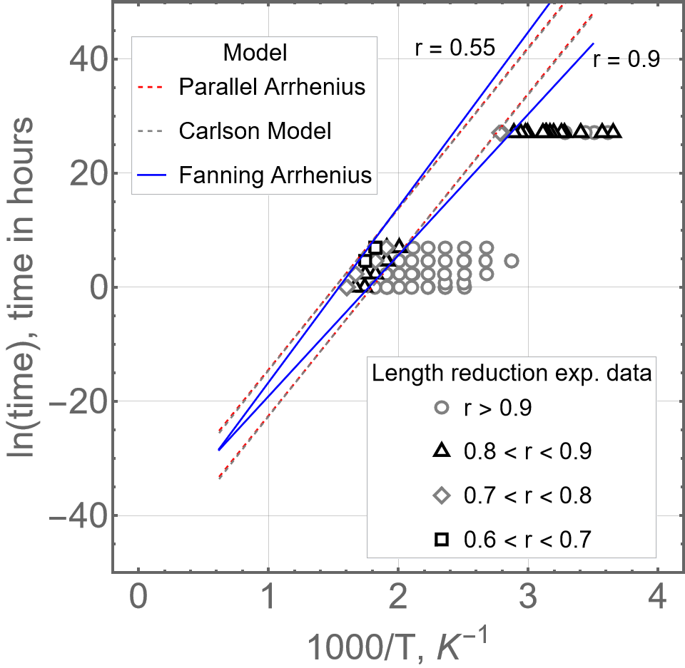
(a)

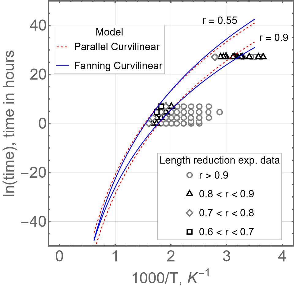
(b)

Figure 1: Representation of the Arrhenius fission-track annealing models in the pseudo-Arrhenius plot. (a) Fanning Arrhenius, Parallel Arrhenius, and Carlson models. (b) Fanning Curvilinear and Parallel Curvilinear models. Laboratory annealing data are c-axis projected reduced fission-track lengths from Durango apatite (Carlson et al., 1999). Data from the geological benchmark KTB (Wauschkuhn et al., 2015) are included only for reference. The models are represented as isoretention curves. Points on these curves are the temperature and time of constant temperature heating resulting in the same reduced length.

The annealing data set on the c-axis projected fission tracks for Durango apatite (Carlson et al., 1999) was used for model fitting. Durango apatite annealing data was chosen because Durango is a well-known standard sample often used in methodological studies (Green et al., 1986; Carlson, 1990; Ketcham et al., 1999, 2007; Rana et al., 2021; Guedes et al., 2022; Rufino and Guedes, 2022). The fitting parameters for PA, PC, FA and FC models are the same presented in Rufino and Guedes (2022). They were numerically determined using the function nlsLM of the package minpack.lm (Elzhov et al., 2016) written in R language, which applies the Levenberg– Marquardt algorithm to minimize the residual sum of square (RSS), using the squared inverse of $r$ uncertainties as weights. With the same method, fitting parameters were also obtained for the CM model. The fitting parameters are presented in the last column of Table 1.

Table 1: Effective reaction rate constant, $r$ reduction and equivalent time equations associated with the fission-track annealing models

FT models	Equations	Parameters (standard error)
Parallel Arrhenius (PA)	$$f_{PA}(t,T)=c_{0}+c_{1}\ln(t)+\frac{c_{2}}{RT}$$ (PA1) $$k_{ef}(T)_{PA}=c_{1}e^{c_{0}/c_{1}}\exp(\frac{c_{2}/c_{1}}{RT})$$ (PA2) $$E_{a}^{PA}=-\frac{c_{2}}{c_{1}}$$ (PA3)	$c_{0}$ = 5.631 (0.220) $c_{1}$ = 0.1865 (0.0066) $c_{2}$ = -10.46 (0.31) kcal/mol $\chi_{\nu}^{2}$ = 2.65
Parallel curvilinear (PC)	$$f_{PC}(t,T)=c_{0}+c_{1}\ln(t)+c_{2}\ln\left(\frac{1}{RT}\right)$$ (PC1) $$k_{ef}(T)_{PC}=c_{1}e^{c_{0}/c_{1}}\left(RT\right)^{-c_{2}/c_{1}}$$ (PC2) $$E_{a}^{PC}(T)=-\frac{c_{2}}{c_{1}}RT$$ (PC3)	$c_{0}$ = -4.910 (0.096) $c_{1}$ = 0.1944 (0.0060) $c_{2}$ = -9.610 (0.244) $\chi_{\nu}^{2}$ = 2.12
Carlson Model (CM)	$$f_{CM}(t,T)=c_{0}+c_{1}\ln(t)+c_{1}\ln(RT)+\frac{c_{2}}{RT}$$ (CM1) $$k_{ef}(T)_{CM}=c_{1}e^{c_{0}/c_{1}}\exp(\frac{c_{2}/c_{1}}{RT})RT$$ (CM2) $$E_{a}^{CM}(T)=-\frac{c_{2}}{c_{1}}+RT$$ (CM3)	$c_{0}$ = 5.426 (0.2155) $c_{1}$ = 0.1867 (0.0066) $c_{2}$ = -10.25 (0.2994) kcal/mol $\chi_{\nu}^{2}$ = 2.63
Fanning Arrhenius (FA)	$$f_{FA}(t,T)=c_{0}+c_{1}\frac{\ln(t)-c_{2}}{\frac{1}{RT}-c_{3}}$$ (FA1) $$k_{ef}(t,T)_{FA}=\frac{c_{1}\exp[(1-n)f_{FA}(t,T)]}{t(1-c_{3}RT)}$$ (FA2) $$E_{a}^{FA}(t,T)=\frac{(RT)^{2}\left[c_{1}(n-1)(c_{2}-\ln t)-c_{3}+1/RT\right]}{(c_{3}RT-1)^{2}}$$ (FA3)	$c_{0}$ = -8.518 (1.072) $c_{1}$ = 0.1266 (0.0191) mol/kcal $c_{2}$ = -20.99 (5.81) $c_{3}$ = 0.2985 (0.1026) mol/kcal $\chi_{\nu}^{2}$ = 1.66 $0.5\leq n<1$
Fanning curvilinear (FC)	$$f_{FC}(t,T)=c_{0}+c_{1}\frac{\ln(t)-c_{2}}{\ln\left(\frac{1}{RT}\right)-c_{3}}$$ (FC1) $$k_{ef}(t,T)_{FC}=\frac{c_{1}\exp[(1-n)f_{FC}(t,T)]}{t\left(\ln\left(\frac{1}{RT}\right)-c_{3}\right)}$$ (FC2) $$E_{a}^{FC}(t,T)=\frac{RT\left(c_{1}c_{2}n-c_{1}c_{2}+(c_{1}-c_{1}n)\ln(t)-c_{3}+\ln\left(\frac{1}{RT}\right)\right)}{\left(c_{3}-\ln\left(\frac{1}{RT}\right)\right)^{2}}$$ (FC3)	$c_{0}$ = -9.449 (1.480) $c_{1}$ = 0.1627 (0.0298) $c_{2}$ = -24.58 (7.75) $c_{3}$ = -0.8626 (0.1549) $\chi_{\nu}^{2}$ = 1.88 $0.5\leq n<1$

Notes: 1. For each fission-track annealing model (Eqs. (PA1), (PC1), (CM1) (FA1), (FC1)), the reaction rate constants, $k_{ef}$ and Arrhenius Activation energies were obtained using $g(r)=\ln(1-r)$ and $f_{r}(r)=(1-r)^{n}$. 2. Rate constants (Eqs. (PA2), (PC2), (CM2) (FA2), (FC2)) were calculated after Eq. (15). 3. Arrhenius activation energies (Eqs. (PA3), (PC3), (CM3) (FA3), (FC3)) were obtained by the application of Eq. (3), and are average values for constant heating experiments.

Fission tracks are formed by displaced atoms and vacant sites, in concentrations high enough to change the structure of the mineral in a volume of about 2-10 nm in diameter and around 20 $\mu$m in length. The annealing process is the recombination of defects and vacancies, which also changes the neighbor structure and consequently the recombination rate. This kind of solid-state reaction is described by the conversion rate equation (Vyazovkin, 2015):

$$\frac{\text{d}\alpha}{\text{d}t}=k(T)f_{\alpha}(\alpha).$$ (5)

The Eq. (5) relates the rate of conversion of the reactant $\alpha$ with the constant rate and with the reaction function $f_{\alpha}(\alpha)$. For the fission tracks, $\alpha$ is the concentration of recombined atoms, and $f_{\alpha}(\alpha)$ describes how the recombination process changes the surrounding structure. The track length can be used as a proxy for the concentration of displaced atoms (Rufino and Guedes, 2022) and:

$$\alpha=\frac{L_{0}-L}{L_{0}}=1-r$$ (6)

and with this change of variable:

$$\frac{\text{d}r}{\text{d}t}=-k_{ef}(t,T)f_{r}(r).$$ (7)

The rate constant has been replaced with an effective rate constant, $k_{ef}(t,T)$, which may depend on time and temperature and is suitable to describe more complex reactions (Vyazovkin, 2016). For the reaction function, the reaction-order function has already been shown to produce consistent results mainly for the single activation energy mechanisms of annealing (Green et al., 1988; Rufino and Guedes, 2022):

$$f_{r}=(1-r)^{n}$$ (8)

in which $n$ is the reaction order.

Eq. (7) is a differential equation that can be solved by the separation of variables. To define the limits of the integral, consider that at the beginning of the thermal history ($t=0$), the track is unannealed ($r=1$). After a heating duration $t$, the track length has been shortened to $r$. Then:

$$\int_{r}^{1}\frac{\text{d}r}{f_{r}(r)}=\int_{0}^{t}-k_{ef}(t,T)\text{d}t.$$ (9)

Eq. (9) is the basic equation from which the annealing kinetics can be studied from a physicochemical perspective. Once the reaction function and the rate constant are chosen, the dependence of the reduced fission-track length can be calculated over any T-t path. Let’s start with the known case of constant temperature heating, from which the annealing equations should be obtained. For the single activation energy models, PA, PC, and CM, the rate constants are given by:

$$k_{ef}(T)_{PA} =A_{1}\exp\left(\frac{-Q_{1}}{RT}\right),$$ (10a)

$$k_{ef}(T)_{PC} =A_{2}(RT)^{m},$$ (10b)

$$k_{ef}(T)_{CM} =A_{3}(RT)\exp\left(-\frac{Q_{3}}{RT}\right),$$ (10c)

where $A_{i}$, $Q_{i}$, and $m$ are constants. Eq. (10a) is the original Arrhenius equation from which the PA equation is derived. $Q_{1}$ can be directly identified with the activation energy only in this case. Eq. (10b) generates the PC equation with a temperature-dependent activation energy (Table 1, Eq. (PC3)). Eq. (10c) generates the Carlson Model, also with a temperature-dependent activation energy (Table 1, Eq. (CM3)). It is the product of Eqs. (10a) and (10b), with $m=1$, and has been proposed soon after the original Arrhenius equation to deal with reactions that deviate from the expected Arrhenius behavior (Kooij, 1893). Note that although the activation energies in the Eqs. (10b) and (10c) depend on temperature, they still fall into the category of single activation energy processes, meaning that all recombination events at a given temperature have the same activation energy.

Annealing experiments are isothermal heating procedures. Then, substituting the effective rate constants (Eqs. (10)) into the integral equation (Eq. 9) together with the reaction-order function defined in Eq. (8) and solving it considering the temperature as a constant results in:

$$\ln(1-r) =\frac{\ln\left[A_{1}(1-n)\right]}{1-n}+\frac{1}{1-n}\ln(t)-\frac{Q_{1}}{1-n}\frac{1}{RT},$$ (11a)

$$\ln(1-r) =\frac{\ln[A_{2}(1-n)]}{1-n}+\frac{1}{1-n}\ln(t)-\frac{m}{1-n}\ln(\frac{1}{RT}),$$ (11b)

$$\ln(1-r) =\frac{\ln\left[A_{3}(1-n)\right]}{1-n}+\frac{1}{1-n}\ln(t)-\frac{Q_{3}}{1-n}\frac{1}{RT}-\frac{1}{1-n}\ln(\frac{1}{RT}),$$ (11c)

which are the equations for the PA (11a), PC (11b), CM (11c) models with $g(r)=\ln(1-r)$. For the chosen reaction function, the integral only has a real solution if $n<1$. Comparing the right sides of these equations respectively with Eqs. (PA1), (PC1), and (CM1), one can find out that the rate constant parameters are related to the fitting parameters of the annealing equations as

$$\text{PA}:n =\frac{c_{1}-1}{c_{1}} Q_{1} =-\frac{c_{2}}{c_{1}} A_{1} =c_{1}\exp(c_{0}/c_{1})$$ (12)

$$\text{PC}:n =\frac{c_{1}-1}{c_{1}} m =-\frac{c_{2}}{c_{1}} A_{2} =c_{1}\exp(c_{0}/c_{1})$$ (13)

$$\text{CM}:n =\frac{c_{1}-1}{c_{1}} Q_{3} =-\frac{c_{2}}{c_{1}} A_{3} =c_{1}\exp(c_{0}/c_{1})$$ (14)

In this way, the rate constants can be expressed in terms of the fitting parameters of the annealing models as shown in Eqs. (PA2), (PC2), and (CM2) of Table 1. The values for the reaction order $n$ for the three models are $n\approx-4$, in agreement with a similar analysis carried out by Green et al. (1988) for the PA model. Therefore, the parallel models are not compatible with first-order annealing kinetics, meaning that the neighbor structure has a strong influence on the rate of defect recombination during annealing.

There are no obvious expressions for the rate constant for the fanning models. A physicochemical analysis of their trends indicates that multiple concurring processes with different activation energies are occurring during the annealing of the fission tracks (Rufino and Guedes, 2022), in agreement with previous suggestions (Green et al., 1988; Tamer and Ketcham, 2020). Rufino and Guedes (2022) derived an expression from Eq. (7) to find the effective rate constant from the annealing model:

$$k_{ef}(t,T)=-\left.\frac{1}{f_{r}(r)}\left[\partialderivative{g(r)}{r}\right]^{-1}\partialderivative{f(t,T)}{t}\right|_{T}$$ (15)

Eq. (15) provides a direct way to calculate this effective reaction rate constant from the model functions that fit the experimental annealing data, $f(t,T)$ and $g(r)$, and from the reaction function $f_{r}(r)$. The partial derivative in relation to time is taken because the annealing models were designed to describe constant temperature experiments. As a check, before applying Eq. (15) to the fanning models, one can show that Eqs. (PA2), (PC2), and (CM2) are found by the application of Eq. (15) respectively to Eqs. (PA1), (PC1), and (CM1), with $g(r)=\ln(1-r)$ and $f_{r}(r)=(1-r)^{n}$. The same procedure can be applied to Eq. (FA1) and (FC1) to find the effective reaction rates respectively for the Fanning Arrhenius (Eq. (FA2)) and Fanning Curvilinear (Eq. (FC2)) models. An alternative way to infer the effective rate constants for the FA and FC models is departing from the hypothesis that the Arrhenius activation energies and, therefore, the rate constants are dependent on the fission-track reduced length. Then, integration of Eq. (9), on the isothermal condition, results in

$$-\int_{1}^{r}\frac{\text{d}r}{f_{r}(r)k_{ef}(r)}=\int_{0}^{t}\text{d}t=t.$$ (16)

It can be shown that the primitive functions that make Eq. (16) true for the FA and FC models, with $f_{r}(r)=(1-n)^{n}$ and $g(r)=\ln(1-r)$ are the ones with the effective rate constants given by Eqs. (FA2) and (FC2). This approach also illustrate how the incorporation of the time in the rate constant and, therefore, in the activation energies for the fanning models are implied from the dependence of the activation energies on the values of $r$.

To obtain the reaction order $n$ for the FA and FC models, the effective reaction rate constants given by Eqs. (FA2) and (FC2) are integrated with Eq. (9) considering constant temperatures (isothermal experiments):

$$\int_{1}^{r}\frac{\text{d}r}{(1-r)^{n}} =-\int_{0}^{t}\frac{c_{1}}{\frac{1}{RT}-c_{3}}\frac{1}{t}\exp\left[-(n-1)\left(c_{0}+c_{1}\frac{\ln t-c_{2}}{\frac{1}{RT}-c_{3}}\right)\right]\text{d}t$$ (17a)

$$\int_{1}^{r}\frac{\text{d}r}{(1-r)^{n}} =-\int_{0}^{t}\frac{c_{1}}{\ln(\frac{1}{RT})-c_{3}}\frac{1}{t}\exp\left[-(n-1)\left(c_{0}+c_{1}\frac{\ln t-c_{2}}{\ln(\frac{1}{RT})-c_{3}}\right)\right]\text{d}t$$ (17b)

With the necessary condition of $n<1$, the solution of the integral equation (17a) is

$$(1-r)=(-1)^{-1/(n-1)}\exp\left[c_{0}+c_{1}\frac{\ln(t)-c_{2}}{\frac{1}{RT}-c_{3}}\right]$$ (18)

As the solution of this equation is to represent the shortening of the fission tracks, $(1-r)$ must be a real value between 0 and 1, which is true only if $-1/(n-1)$ is an even and positive integer value $2j$. Then, the values of $n$ are restricted to

$$n=\frac{2j-1}{2j},$$ (19)

where $j=1,2,3,...$. With this condition and $g(r)=\ln(1-r)$, the FA model (Table 1, Eq.(FA1)) is recovered. The solutions for Eqs. (17a) and (17b) are similar, differing only on the logarithm of $1/RT$ for the FC model instead of the $1/RT$ for the FA model, which are both constants in this case. The previous analysis holds also for the FC model. The values of $n$ will be fractional for FA and FC ($n=1/2,3/4,5/6,7/8,...$), according to Eq. (19). Fractional reaction orders are characteristics of multiple-step reactions or some more complex kinetic mechanism, as it has been explained for the decomposition of acetaldehyde (Laidler et al., 1965), a well know example of fractional reaction order in chemistry. However, for the fission tracks, where the displaced atoms and vacant sites take the role of reactants and the deformed track structure is the reaction medium, explanations of the kinetics of a single reactant via a mean-field approximation (MFA) may not be appropriate (Córdoba-Torres et al., 2003). Thus, for the effective reaction rate constant $k_{ef}$ of the fanning annealing models, mechanistic modeling considering the intermediate steps, i.e., recognizing the reaction order of each mechanism involved in annealing, would be desirable to elucidate the meaning of the fractional reaction order found (Koga et al., 1992). The rate constants for FA and FC are to be viewed as effective equations constraining the general behavior of annealing but that does not allow the description of the specifics of the annealing kinetics.

In this physicochemical framework of the fission-track annealing, the effective reaction rate constant, $k_{ef}(t,T)$, and the reaction function, $f_{r}(r)$, are the fundamental building blocks from which the fission-track annealing kinetics can be studied. The application to the constant temperature annealing made it possible to determine the rate constant parameters from the empirically determined parameters of the annealing equations. The calculation of the Arrhenius activation energies ($E_{a}$) for different models becomes possible through Eq. (3). The Arrhenius activation energies of the parallel annealing models (Eq. PA3, PC3 and CM3) will be constants with respect to the variable $t$. As for the fanning equations, $E_{a}$ will vary with time and temperature (Eq. FA3 and FC3). However, the main advantage of this approach is the possibility of calculating the fission-track length reduction over any T-t path using Eq. (9), without recurring to the interactive application of the Principle of Equivalent Time.

2.2 Fission track annealing under variable temperature thermal histories

Fission-track thermal history inference is based on the Principle of Equivalent Time (PET) (Goswami et al., 1984; Duddy et al., 1988), which is an interactive method that allows the application of isothermal annealing models to variable temperature T-t paths. It is detailed in Appendix A. In general, a given variable temperature thermal history is divided into finite time intervals $\Delta t_{i}$, centered at times $t_{i}$ and temperatures $T_{i}$. At the time interval in which the population was born, a first reduced length is calculated by applying the annealing equation, using the temperature of the T-t path and the duration of the interval ($T_{i},\Delta t_{i}$). In the next interval, at a different temperature on T-t path, the annealing model is used to find an equivalent time capable of producing the same length shortening of the previous interval but at the new temperature. A new length shortening is then calculated by applying the annealing model to the period of time that is the sum of the equivalent time and the length of the time interval. This procedure is repeated and at any given temperature, $T_{i}$ on the T-t path, an equivalent time, $\tau_{i}$, which reproduces the length shortening at the previous interval, $r_{i-1}$, is determined, so that the new length shortening can be calculated as if the track had been at the same constant temperature from the beginning. The reduced length is updated ($r_{i}$) by calculating it as a result of heating at $T_{i}$ for the duration $\tau_{i}+\Delta t_{i}$. The hypothesis that the annealing kinetics does not depend on the previous thermal history of the track, but only on its current length so that any previous T-t path can be replaced with a constant temperature heating resulting in this length, is the basis of this procedure and defines the Principle of Equivalent Time. This means, in practice, that the track will have no memory of the material conditions of time and temperature of its previous shortenings. The equations for the application of the PET with the PA, PC, CM, FA, and FC models can be found in Table A1 in Appendix A.

The physicochemical tool presented in the previous section provides an alternative way to access variable temperature annealing kinetics by solving the integral in the right side of Eq. (9) over a T-t path. Eq. (9) is solved as a line integral. A suitable parameterization is:

$$s=\begin{cases}T=T(u)\\ t=u\end{cases},\\ \text{d}s=\sqrt{1+\left(\frac{\text{d}T}{\text{d}u}\right)^{2}}\text{d}u.$$ (20)

Implementing the parameterized variables on the right side of the integral equation (Eq. 9),

$$I=\int_{0}^{t}k_{ef}\left(t(u),T(u)\right)\frac{\text{d}s}{\sqrt{1+\left(\frac{\text{d}T}{\text{d}u}\right)^{2}}}\implies I=\int_{0}^{t}k_{ef}\left(t(u),T(u)\right)\text{d}u.$$ (21)

Solving the left side of Eq. (9) for the $f_{r}(r)$ function given by Eq. (8) and the parameterized integral for the rate constant (Eq. (21)), the reduced length, after the track has experienced the thermal history given by the T-t path, is

$$r=1-\left((1-n)\int_{0}^{t}k_{ef}\left(t(u),T(u)\right)\text{d}u\right)^{1/1-n},$$ (22)

in which $n<1$ as usual. At a first glance, the advantage of the Rate Constant path Integral (RCI, Eq. (22)) is that it is a one-shot calculation of the reduced track length. In addition, there was no need to restrict the form of the rate constant function and therefore the annealing mechanism it is related to.

3 Results and Discussion

The RCI Eq. (22) can be applied to calculate the shortening in the reduced length of a single fission-track population submitted to any T-t path. The same calculation can be carried out using the interactive technique based on the Principle of Equivalent Time (PET). To compare the outcomes of the two methods, both calculations will be performed for the parallel (including CM) and fanning models. The case will be made for the linear cooling, $T(t)=T_{0}-\dot{T}t$, where $\dot{T}$ is the cooling rate and $T_{0}$ is the temperature at the time the track was generated. The temperature at the end of the T-t path (present time) was fixed to be 20 ^∘C (293.15 K) for this analysis.

3.1 Parallel models

To solve the RCI, the effective rate constant functions for the parallel models (Table 1, Eqs. (PA2), (PC2), and (CM2)) are inserted in Eq. (22) with the variable $T$ replaced with $T(t)=T_{0}-\dot{T}t$ wherever it appears. The analytical solutions for the reduced length shortening calculated for the PA, PC, and CM are

$$r_{PA} =1-\left(\frac{e^{c_{0}/c_{1}}\left(c_{2}\text{Ei}\left(\frac{c_{2}}{c_{1}R(T_{0}-\dot{T}t)}\right)-c_{2}\text{Ei}\left(\frac{c_{2}}{c_{1}RT_{0}}\right)+c_{1}R\left((\dot{T}t-T_{0})e^{\frac{c_{2}}{c_{1}R(T_{0}-\dot{T}t)}}+T_{0}e^{\frac{c_{2}}{c_{1}RT_{0}}}\right)\right)}{c_{1}\dot{T}R}\right)^{c_{1}},$$ (23a)

$$r_{PC} =1-\left(\frac{c_{1}e^{c_{0}/c_{1}}\left((\dot{T}t-T_{0})(R(T_{0}-\dot{T}t))^{-\frac{c_{2}}{c_{1}}}+T_{0}(RT_{0})^{-\frac{c_{2}}{c_{1}}}\right)}{c_{1}\dot{T}-c_{2}\dot{T}}\right)^{c_{1}},$$ (23b)

$$\begin{split}r_{CM}=1-2^{-c_{1}}e^{c_{0}}\frac{c_{1}^{-2c_{1}}}{(\dot{T}R)^{c_{1}}}\left[c_{1}R\left(T_{0}e^{\frac{c_{2}}{c_{1}RT_{0}}}(c_{1}RT_{0}+c_{2})-(T_{0}-\dot{T}t)e^{\frac{c_{2}}{c_{1}RT_{0}-c_{1}\dot{T}Rt}}(c_{1}R(T_{0}-\dot{T}t)+c_{2})\right)\right.\\ +c_{2}^{2}\left.\left(\text{Ei}\left(\frac{c_{2}}{c_{1}RT_{0}-c_{1}Rt\dot{T}}\right)-\text{Ei}\left(\frac{c_{2}}{c_{1}RT_{0}}\right)\right)\right]^{c_{1}},\end{split}$$ (23c)

where Ei is the exponential integral function. Eqs. (23a) - (23c) give the resulting reduced length $r$ for the parallel models, as functions of the three variables that characterize the thermal history: the duration of the T-t path ($t$), the cooling rate ($\dot{T}$), and the temperature at the time when the track was born ($T_{0}$). The parameters $c_{i}$ are given in the last column of Table 1. The values of $r$ for the cooling path with the cooling rate $\dot{T}=1.0^{\circ}$C/Ma calculated with the three parallel models are presented in Fig. 2. For each point, the value of $r$ is the length reduction after a linear cooling duration $t$ and measured in the present. Values of $r=0$ mean that the tracks have been erased before the present. Values obtained by the RCI solutions (Eqs. (23a) - (23c)) are represented as red curves marked with red circles and the values calculated using the PET are represented as blue curves marked with blue squares. RCI and PET calculations produce very close values of $r$ for the three parallel models (Figs. 2(a), 2(b), 2(c)).

,

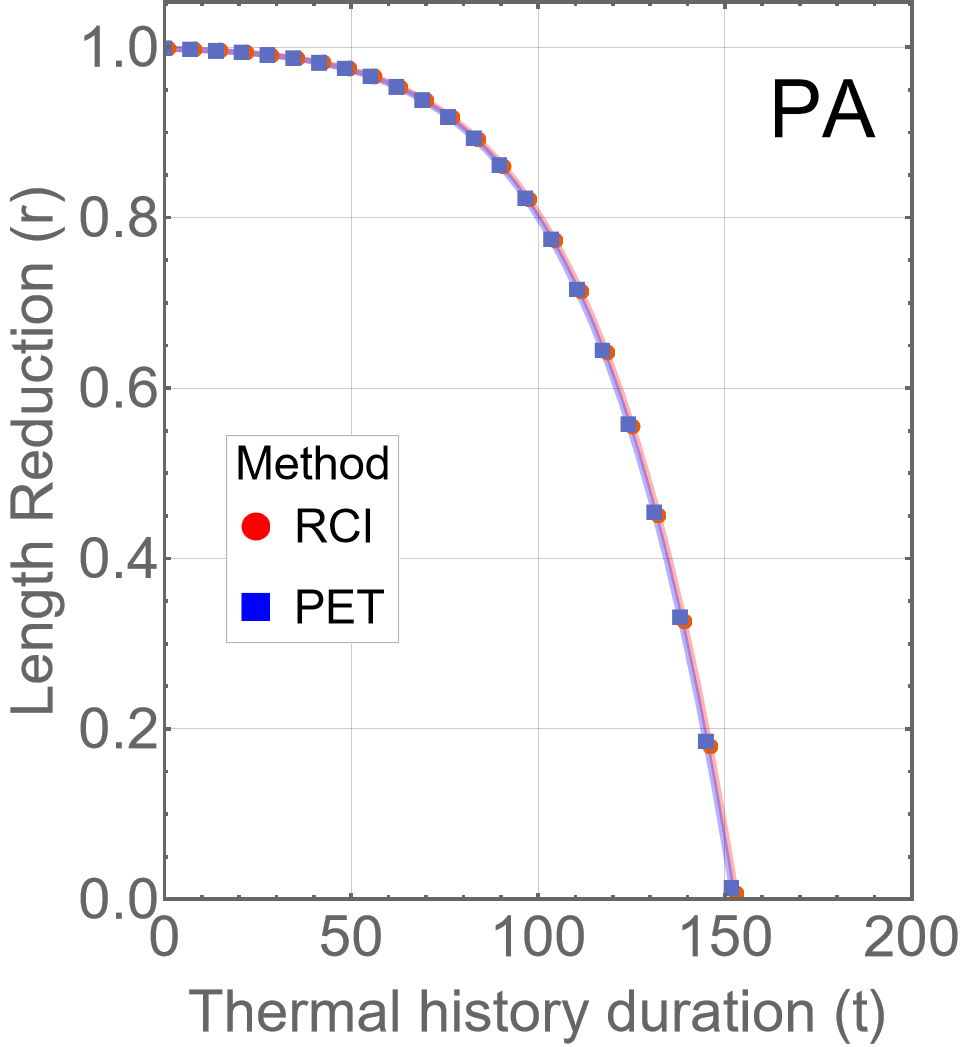
(a)

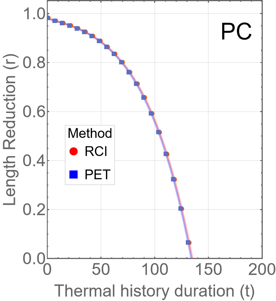
(b)

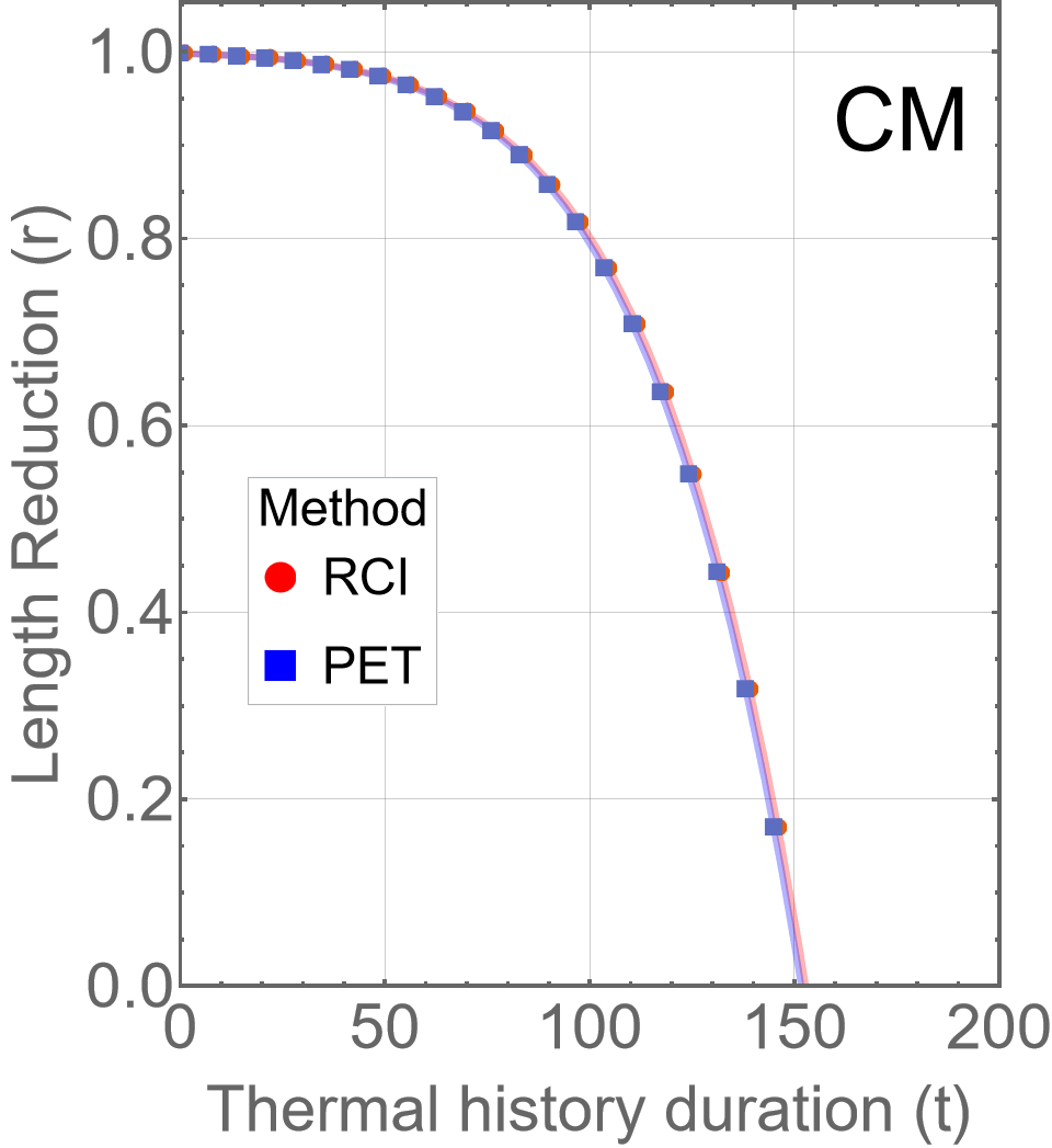
(c)

Figure 2: Values of the reduced track lengths ($r$), after a linear cooling ($\dot{T}=1.0^{\circ}$C/Ma) starting at time $t$ and ending at the present time at a fixed temperature of 20^∘C, calculated using the Parallel models: (a) Arrhenius, (b) Curvilinear, and (c) Carlson). The points that form the curve in red (circle marks) were calculated by applying the RCI (Eq. 23a, 23b, and 23c). The values calculated using the PET are in blue (square marks).

The temperature indexes Closure Temperature ($T_{C}$) and Total Annealing Temperature ($T_{A}$) were also calculated for the three parallel models, applying both methods of calculation, for cooling T-t paths with cooling rates of 1, 10, and 100 ^∘C/Ma. $T_{C}$ is, for a monotonic cooling thermal history, the temperature at the apparent sample age (Dodson, 1973). $T_{A}$ is the age of the oldest track that has not been erased and can be counted in the sample (Issler, 1996). Details for the method of calculation of the index temperatures can be found in Guedes et al. (2013). $T_{C}$ and $T_{A}$ are meaningful quantities that allow quantifying the impact of using the RCI instead of the interactive PET calculation. The uncertainties in $T_{C}$ and in $T_{A}$ were estimated by simple error propagation of apparent ($T_{C}$) or retention ($T_{A}$) ages and present time temperature. Results are shown in Table 2. Setting the PET results as the reference values, given that PET is the method established in the literature, a relative error analysis can be carried out to verify the internal consistency between PET and RCI calculations. The relative error between PA PET and PA RCI is on average 0.69$\%$ for $T_{C}$ and 1.19$\%$ $T_{A}$. The same trend is found for calculations of $T_{C}$ and $T_{A}$ with PC and CM: 0.66$\%$ and 0.58$\%$ (PC) and 0.7$\%$ and 1.19$\%$ (CM). All errors are well inside the estimated uncertainties for temperature index values and are most probably artifacts of the PET numerical calculation.

Table 2: Comparison of thermal indexes for the models presented in this work, calculated using the PET and the RCI

Principle of Equivalent Time (PET) thermal indexes
Fit	$T_{C}$1	$T_{C}$10	$T_{C}$100	$T_{A}$1	$T_{A}$10	$T_{A}$100
PA	130(7)	144(7)	158(8)	153(8)	168(8)	184(9)
PC	105(6)	121(6)	139(7)	132(8)	151(8)	171(9)
CM	130(7)	143(7)	157(8)	153(8)	168(8)	184(9)
FA	134(7)	146(7)	160(8)	163(8)	176(8)	191(10)
FC	111(6)	126(6)	143(7)	143(7)	160(8)	179(9)
Rate constant integral on a path (RCI) thermal indexes
Fit	$T_{C}$1	$T_{C}$10	$T_{C}$100	$T_{A}$1	$T_{A}$10	$T_{A}$100
PA	131(7)	145(7)	159(8)	155(8)	170(8)	186(9)
PC	106(6)	122(6)	140(7)	133(8)	152(7)	172(9)
CM	131(7)	144(7)	158(8)	155(8)	170(8)	186(9)
FA	125(7)	137(7)	150(7)	153(9)	166(8)	181(10)
FC	100(6)	115(6)	130(6)	130(8)	148(8)	165(8)

Notes: 1. Temperatures in ^∘C. 2. The standard errors are given in parentheses. 3. $T_{C}$: Closure Temperature. 4. $T_{A}$: Total Annealing Temperature. 5. The numbers to the right of $T_{C}$ and $T_{A}$ are the cooling rates in ^∘C/Ma.

The PET was formulated under the hypothesis that the annealing of fission tracks is a single activation energy process Duddy et al. (1988). The internal consistency between PET and RCI values of $r$, $T_{C}$, and $T_{A}$ calculated with the parallel models is a check for the robustness of the physicochemical approach to deal with variable temperature thermal histories. It is to be noted that not only the PA model, in which the activation energy is temperature-independent (Table 1, Eq. (PA3)), but also the PC model, in which the activation energy is temperature-dependent (Table 1, Eqs. (FC3)), show such internal consistency. The same agreement is observed for CM. The CM activation energy may vary with temperature but, with the parameters shown in Table 1, its Arrhenius activation energy is approximately constant since the value of $c_{2}/c_{1}$ (54.9 kcal/mol) is much higher than typical values of $RT$ (< 1.0 kcal/mol). Although the activation energies may vary with temperature, these models imply that at any given temperature, the recombination events are taking place with the same activation energy. This is a sufficient condition for the applicability of the PET.

3.2 Fanning models

The values of $r$, $T_{C}$, and $T_{A}$ for the cooling T-t path were also calculated for the fanning models, using both the interactive PET and RCI methods. However, the RCI (Eq. (22)) could not be solved analytically for the FA and FC rate constants (Table 1, Eqs. (FA2) and (FC2)). The integrals were then solved numerically with the Wolfram Mathematica software (Wolfram-Research-Inc., 2021). For validation, the integrals for the parallel models were also solved numerically resulting in exactly the same values obtained with the analytical solutions (Eqs. (23a)-(23c)). Another feature to be considered is that there are certain fractional values allowed for the reaction order $n$, given by Eq. (19). The analysis will be limited to $n=0.5$, $n=0.75$ and $n=0.9$. The numerical method breaks down when $n>0.95$ although its mathematical upper bound is $n<1$. The reduced length calculation results are shown in Fig. 3. Values calculated with the PET are shown in blue, with triangle marks, while values found by solving the RCI are shown, in red ($n=0.5$), purple ($n=0.75$), and light purple ($n=0.9$), respectively with circle, square, and diamond marks. RCI $r$ curves are very close to each other but depart from the $r$ values calculated with the PET. Significant differences between RCI and PET $r$ values are observed for the FC (Fig. 3(b)) and for the FA (Fig. 3(a)) models.

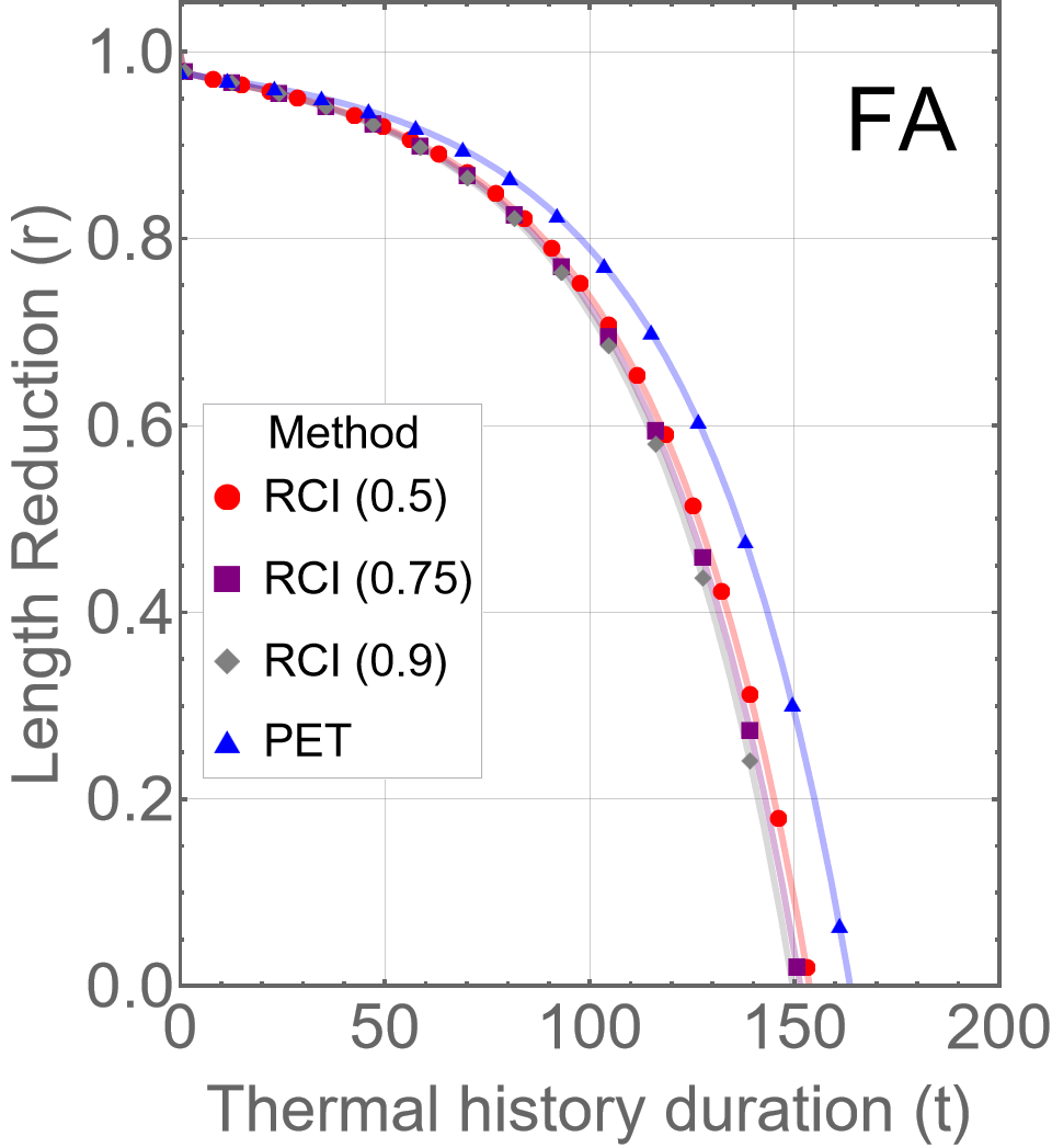
(a)

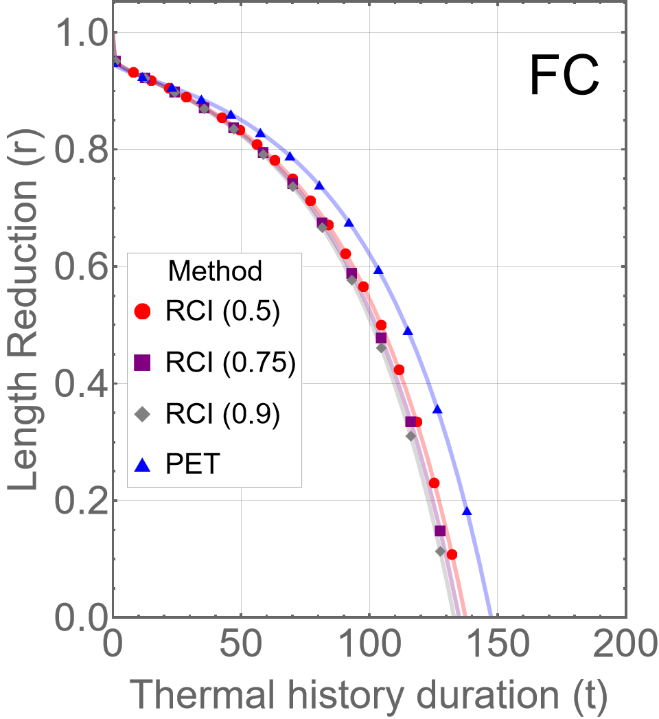
(b)

Figure 3: Values of the reduced track lengths ($r$), after a linear cooling ($\dot{T}=1.0^{\circ}$C/Ma) starting at time $t$ and ending at the present time at a fixed temperature of 20^∘C, calculated using the Fanning models: (a) Arrhenius and (b) Curvilinear. The points that form the curves in red (circle marks), purple (square marks), and light purple (diamond marks) were calculated by applying the RCI, respectively with $n=0.5$, $n=0.75$, and $n=0.9$. The values calculated using the PET are in blue.

The values of $T_{C}$ and $T_{A}$ for the fanning models, calculated using the PET and the RCI ($n=0.5$) are in Table 2. For the FA model, the mean relative errors between the PET and the RCI $T_{C}$ and $T_{A}$ calculations are respectively 6.25$\%$ and 5.68$\%$. For the FC model, the same comparisons result in still more significant differences: 9.57$\%$ ($T_{C}$) and 8.48$\%$ ($T_{A}$). The deviations between the values calculated using the PET and the RCI are much more significant than the ones found for the parallel model calculations. One major issue is that the fanning models do not fulfill the single activation energy hypothesis on which the PET is founded. The fanning models emerge from multiple concurring processes with different activation energies (Tamer and Ketcham, 2020; Rufino and Guedes, 2022). The effective Arrhenius activation energies incorporate a time dependence (Table 1, Eqs. (FA3) and (FC3)) that is the consequence of their dependence on the current reduced fission-track length (different slopes of the isoretention curves in the pseudo-Arrhenius plot). On the other hand, the rate constant integral (Eq. (22)) was obtained in a physicochemical framework developed to deal with chemical reactions that did not fit the single activation energy Arrhenius law (Vyazovkin, 2015). It is by design suitable for complex activation energy systems like the ones pictured by the fanning models. Note also that the presented figures are particular of the fitting parameters in Table 1. A different set of parameters would result in different values without changing the conclusion that RCI and PET predictions deviate from each other.

3.3 Implications for the thermal history modeling

The fanning models, especially the Fanning Curvilinear, have been shown to produce better fits to laboratory data and better geological extrapolation of annealing effects (Ketcham et al., 2007; Guedes et al., 2013). However, the application of the FC along with the PET is an approximation. Compared with the RCI formulation, it underestimates the annealing effect in about 10$\%$, i.e., it predicts that higher temperatures are necessary for the same length shortening as calculated with the RCI for the tested cooling histories. In the context of the inverse problem of inferring T-t paths from the FT age and track length distribution of a mineral sample, it implies the requirement of a longer residence time in the partial annealing zone. For instance, compare, in Table 2, the FC $T_{A}$ calculated with RCI for a cooling rate of 10^∘C/Ma (148^∘C) with the FC $T_{A}$ calculated with PET for a cooling rate of 1^∘C/Ma (143^∘C). The same analysis applies to the FA model with less significant relative error figures (about 6$\%$).

The Parallel models (PA, PC, and CM), which can be safely applied along with the PET, have long been ruled out for FTT studies (Laslett et al., 1987; Guedes et al., 2013; Ketcham et al., 1999, 2007; Ketcham, 2019). Duddy et al. (1988) had argued that the FA deviated only slightly from the PA model and applied it along with the PET. The isoretention curves for the two models follow approximately the same trends (Fig. 1(a)). The same behavior is observed for the curvilinear models (Fig. 1(b)). FC and PC isoretention curves bend together towards lower temperatures. Their argument can be better appreciated in Fig. 4. All the PET and RCI predictions for reduced lengths after the track underwent the cooling history are gathered in the same plot. Note that the linear models (PA and FA) and the approximately linear CM form a cluster, while the curvilinear models (PC and FC) form a separate set. The predictions with the fanning models and PET are closer to the predictions of the parallel models for track populations born when the sample passed through intermediate temperatures (partial annealing zone), which results in closer $T_{C}$ values (compare values in Table 2). For populations born at higher temperatures, the fanning-PET predictions depart from the parallel model ones, resulting in a more significant difference between calculated $T_{A}$ values. Calculations with RCI approximate fanning and parallel model predictions for populations born at higher temperatures. Within this approximation, it could be possible to engineer fanning model parameters to make the model even closer to a parallel model.

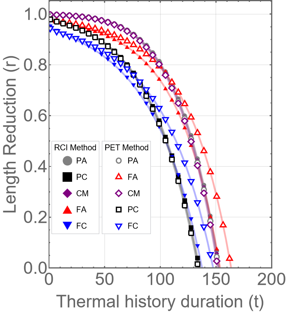
Figure 4: Values of the reduced track lengths ($r$), after a linear cooling ($\dot{T}=1.0^{\circ}$C/Ma) starting at time $t$ and ending at the present time at a fixed temperature of 20^∘C, calculated for the parallel and fanning models. Calculations using RCI are shown as solid geometric forms, while calculations using PET are represented by empty geometric forms.

4 Concluding remarks

Departing from Eq. (9), a physicochemical framework was built to deal with the effects of annealing in variable temperature T-t paths. The basic building blocks are the reaction function $f_{r}(r)$ and the effective rate constant, $k_{ef}(t,T)$. The parallel models (PA, PC, and CM) were shown to be consistent with the single activation energy rate constants given by Eqs. (10a)-(10c) and with the reaction-order function (Eq. (8)). The fanning models (FA and FC) are the representation of multiple concurrent recombination processes with different activation energies (Rufino and Guedes, 2022). The $k_{ef}(t,T)$ functions were built (Eq. (15)) to be consistent with the reaction-order function (Eq.(8)). Obtaining FA and FC rate constants from first principle, i.e., a composition of rate constants for individual processes, and validating them experimentally is still an open issue that has to be dealt with. The Eq. (22) is the line integral related to Eq. (9) from which length shortening due to cooling T-t paths can be directly calculated, independently of whether the rate constant represents a single or multiple activation energy mechanism.

The Principle of Equivalent Time, on the other hand, is only valid for single activation energy equations, which, for the fission-track system, are the parallel models. In these cases, the RCI-based calculations are in agreement with the PET ones (Fig. 2), indicating the robustness of RCI formulation. For the fanning models, the use of the PET has long been recognized as an approximation (Duddy et al., 1988). Deviations have indeed been observed between RCI and PET-based calculations (Fig. 3). Compared to the application of RCI, the PET calculation underestimates annealing effects in variable temperature T-t paths (Table 2).

The PET along with FA or FC models is the calculation method used to infer most published thermal histories. This procedure introduces a systematic deviation that should be considered in the geological interpretation of the thermal history modeling. Alternatively, the rate constant integral (Eq. (22)) could be considered to substitute the PET in inversion thermal history codes (Ketcham, 2005; Gallagher, 2012). Computationally, solving an integral, even numerically, is a routine faster than the interactive steps necessary to apply the PET. More importantly, if the rate constants are representative of the track annealing kinetics, this framework results, in principle, in more accurate predictions of the annealing effects in samples submitted to variable temperature thermal histories.

Appendix

Appendix A Equations for the application of the Principle of Equivalent Time

Table A1: Equations for the application of the Principle of Equivalent Time

FT models	Equations	Parameters (standard error)
Parallel Arrhenius (PA)	$$\ln\left(1-r_{j-1}\right)=1-\exp\left[f_{PA}\left(\text{$\Delta$t}_{j}+\tau_{r_{j-1}},T_{j}\right)\right]$$ (PA4) $$\ln(\tau_{r_{j-1}})=\frac{\ln\left(1-r_{j-1}\right)}{c_{1}}-\frac{c_{2}}{c_{1}RT_{j}}-\frac{c_{0}}{c_{1}}$$ (PA5)	$c_{0}$ = 5.631 (0.220) $c_{1}$ = 0.1865 (0.0066) $c_{2}$ = -10.46 (0.31) kcal/mol $\chi_{\nu}^{2}$ = 2.65
Parallel curvilinear (PC)	$$\ln\left(1-r_{j-1}\right)=1-\exp\left[f_{PC}\left(\text{$\Delta$t}_{j}+\tau_{r_{j-1}},T_{j}\right)\right]$$ (PC4) $$\ln(\tau_{r_{j-1}})=\frac{\ln\left(1-r_{j-1}\right)}{c_{1}}-\frac{c_{2}}{c_{1}}\ln\left(\frac{1}{RT_{j}}\right)-\frac{c_{0}}{c_{1}}$$ (PC5)	$c_{0}$ = -4.910 (0.096) $c_{1}$ = 0.1944 (0.0060) $c_{2}$ = -9.610 (0.244) $\chi_{\nu}^{2}$ = 2.12
Carlson Model (CM)	$$\ln\left(1-r_{j-1}\right)=1-\exp\left[f_{CM}\left(\text{$\Delta$t}_{j}+\tau_{r_{j-1}},T_{j}\right)\right]$$ (CM4) $$\ln(\tau_{r_{j-1}})=\frac{\ln\left(1-r_{j-1}\right)}{c_{1}}-\frac{c_{2}}{c_{1}RT_{j}}-\frac{c_{0}}{c_{1}}-\ln\left(RT_{j}\right)$$ (CM5)	$c_{0}$ = 5.426 (0.2155) $c_{1}$ = 0.1867 (0.0066) $c_{2}$ = -10.25 (0.2994) kcal/mol $\chi_{\nu}^{2}$ = 2.63
Fanning Arrhenius (FA)	$$\ln\left(1-r_{j-1}\right)=1-\exp\left[f_{FA}\left(\text{$\Delta$t}_{j}+\tau_{r_{j-1}},T_{j}\right)\right]$$ (FA4) $$\ln(\tau_{r_{j-1}})=\frac{\left[\ln\left(1-r_{j-1}\right)-c_{0}\right]\left[\frac{1}{RT_{j}}-c_{3}\right]}{c_{1}}+c_{2}$$ (FA5)	$c_{0}$ = -8.518 (1.072) $c_{1}$ = 0.1266 (0.0191) mol/kcal $c_{2}$ = -20.99 (5.81) $c_{3}$ = 0.2985 (0.1026) mol/kcal $\chi_{\nu}^{2}$ = 1.66
Fanning curvilinear (FC)	$$\ln\left(1-r_{j-1}\right)=1-\exp\left[f_{FC}\left(\text{$\Delta$t}_{j}+\tau_{r_{j-1}},T_{j}\right)\right]$$ (FC4) $$\ln(\tau_{r_{j-1}})=\frac{\left[\ln\left(1-r_{j-1}\right)-c_{0}\right]\left[\ln(\frac{1}{RT_{j}})-c_{3}\right]}{c_{1}}+c_{2}$$ (FC5)	$c_{0}$ = -9.449 (1.480) $c_{1}$ = 0.1627 (0.0298) $c_{2}$ = -24.58 (7.75) $c_{3}$ = -0.8626 (0.1549) $\chi_{\nu}^{2}$ = 1.88

Notes: 1. For each fission-track annealing model (Eqs. (PA1), (PC1), (FA1), (FC1)), the length reduction $r$ (Eqs. (PA4), (PC4), (FA4), (FC4)) and equivalent time $\tau$ (Eqs. (PA5), (PC5), (FA5), (FC5)) were obtained using $g(r)=\ln(1-r)$.

The proposed method to deal with annealing in thermal histories with variable temperatures is also based on the Arrhenius equation and was first proposed by Goswami et al. (1984). The Principle of Equivalent Time (PET), on which this method is founded, states that the annealing rate of a track does not depend on its previous thermal history, but only on its current length.

The procedure to solve this problem is to infer the magnitude of annealing recursively, dividing the thermal history into appropriate intervals $\Delta t_{i}$ and starting from a given value of $r$. For each step, annealing is carried out at constant temperature. In the first step, centered at $(t_{1},T_{1})$. The procedure will be shown for the Parallel Arrhenius model. The reduced fission-track length is calculated using Eq. (PA1), along with $g(r)=\ln(1-r)$:

$$r_{1}=1-(\Delta t_{1})^{c_{1}}\exp(c_{0}+\frac{c_{2}}{RT_{1}})$$ (24)

For the next step, the calculation of $r_{2}$ incorporates the principle in the form that this new shortening is postulated to be independent of the previous one. Thus, one can find a length of time, $\tau_{r_{1}}$, that will yield the length $r_{1}$ but for heating at the temperature of the second interval, $T_{2}$:

$$\tau_{r_{1}}=(1-r_{1})^{-1/c_{1}}\exp(-\frac{1}{RT_{2}}\frac{c_{2}}{c_{1}}+\frac{c_{0}}{c_{1}}).$$ (25)

The value of $r_{2}$ is then found by the application of the annealing model to the interval $\tau_{r_{1}}+\Delta t_{2}$:

$$r_{2}=1-(\tau_{r_{1}}+\Delta t_{2})^{c_{1}}\exp(c_{0}+\frac{c_{2}}{RT_{2}}).$$ (26)

This procedure is interactively repeated for the entire T-t path. The last value of $r$ will be the reduced length of the population born in the first interval after experiencing the entire thermal history. For each interval $j$, the formulas above are:

$$r_{j} =1-(\tau_{r_{j-1}}+\Delta t_{j})^{c_{1}}\exp(c_{0}+\frac{c_{2}}{RT_{j}})$$ (27a)

$$\tau_{r_{j-1}} =(1-r_{j-1})^{-1/c_{1}}\exp(-\frac{1}{RT_{j}}\frac{c_{2}}{c_{1}}+\frac{c_{0}}{c_{1}})$$ (27b)

The formulas for the PA, PC, CM, FA, and FC models are presented in Table A1.

References

- Arrhenius (1889) Arrhenius, S., 1889. Über die reaktionsgeschwindigkeit bei der inversion von rohrzucker durch säuren. Zeitschrift für Physikalische Chemie 4, 226–248. URL: https://www.degruyter.com/view/journals/zpch/4U/1/article-p226.xml.
- Carlson (1990) Carlson, W.D., 1990. Mechanisms and kinetics of apatite fission-track annealing. American Mineralogist 75, 1120–1139. URL: <GotoISI>://WOS:A1990EL25100017. times Cited: 116 Carlson, wd Carlson, William/A-5807-2008 Carlson, William/0000-0002-2954-5886 121.
- Carlson et al. (1999) Carlson, W.D., Donelick, R.A., Ketcham, R.A., 1999. Variability of apatite fission-track annealing kinetics: I. experimental results. American Mineralogist 84, 1213–1223. URL: <GotoISI>://WOS:000082349700001. times Cited: 346 Carlson, WD Donelick, RA Ketcham, RA Ketcham, Richard/B-5431-2011; Carlson, William/A-5807-2008 Ketcham, Richard/0000-0002-2748-0409; Carlson, William/0000-0002-2954-5886 370.
- Cohen et al. (2007) Cohen, E., Cvitas, T., Fry, J., et al., 2007. Iupac quantities, units and symbols in physical chemistry. IUPAC and RSC Publishing, Cambridge .
- Córdoba-Torres et al. (2003) Córdoba-Torres, P., Nogueira, R.P., Fairén, V., 2003. Fractional reaction order kinetics in electrochemical systems involving single-reactant, bimolecular desorption reactions. Journal of Electroanalytical Chemistry 560, 25–33.
- Crowley et al. (1991) Crowley, K.D., Cameron, M., Schaefer, R.L., 1991. Experimental studies of annealing of etched fission tracks in fluorapatite. Geochimica Et Cosmochimica Acta 55, 1449–1465. URL: <GotoISI>://WOS:A1991FM71600019, doi:10.1016/0016-7037(91)90320-5. times Cited: 187 Crowley, kd cameron, m schaefer, rl 210.
- Dodson (1973) Dodson, M.H., 1973. Closure temperature in cooling geochronological and petrological systems. Contributions to Mineralogy and Petrology 40, 259–274.
- Duddy et al. (1988) Duddy, I., Green, P., Laslett, G., 1988. Thermal annealing of fission tracks in apatite 3. variable temperature behaviour. Chemical Geology: Isotope Geoscience section 73, 25–38.
- Elzhov et al. (2016) Elzhov, T.V., Mullen, K.M., Spiess, A.N., Bolker, B., 2016. minpack.lm: R Interface to the Levenberg-Marquardt Nonlinear Least-Squares Algorithm Found in MINPACK, Plus Support for Bounds. URL: https://CRAN.R-project.org/package=minpack.lm. r package version 1.2-1.
- Gallagher (2012) Gallagher, K., 2012. Transdimensional inverse thermal history modeling for quantitative thermochronology. Journal of Geophysical Research-Solid Earth 117. URL: <GotoISI>://WOS:000301136400002, doi:10.1029/2011jb008825.
- Goswami et al. (1984) Goswami, J., Jha, R., Lal, D., 1984. Quantitative treatment of annealing of charged particle tracks in common minerals. Earth and Planetary Science Letters 71, 120–128.
- Green et al. (1988) Green, P., Duddy, I., Laslett, G., 1988. Can fission track annealing in apatite be described by first-order kinetics? Earth and Planetary Science Letters 87, 216–228.
- Green et al. (1986) Green, P.F., Duddy, I.R., Gleadow, A.J.W., Tingate, P.R., Laslett, G.M., 1986. Thermal annealing of fission tracks in apatite .1. a qualitative description. Chemical Geology 59, 237–253. URL: <GotoISI>://WOS:A1986F612200002, doi:10.1016/0009-2541(86)90048-3.
- Guedes et al. (2022) Guedes, S., Lixandrão Filho, A.L., Hadler, J.C., 2022. Generalization of the fission-track arrhenius annealing equations. Mathematical Geosciences , 1–20.
- Guedes et al. (2013) Guedes, S., Moreira, P.A., Devanathan, R., Weber, W.J., Hadler, J.C., 2013. Improved zircon fission-track annealing model based on reevaluation of annealing data. Physics and Chemistry of Minerals 40, 93–106.
- Guedes et al. (2006) Guedes, S., Oliveira, K., Moreira, P., Iunes, P., et al., 2006. Kinetic model for the annealing of fission tracks in minerals and its application to apatite. Radiation measurements 41, 392–398.
- Issler (1996) Issler, D., 1996. Optimizing time step size for apatite fission track annealing model. Computers and Geosciences 22, 835–835.
- Ketcham (2005) Ketcham, R.A., 2005. Forward and inverse modeling of low-temperature thermochronometry data. volume 58 of Reviews in Mineralogy and Geochemistry. pp. 275–314. URL: <GotoISI>://WOS:000235184200011, doi:10.2138/rmg.2005.58.11.
- Ketcham (2019) Ketcham, R.A., 2019. Fission-Track Annealing: From Geologic Observations to Thermal History Modeling. Springer International Publishing, Cham. pp. 49–75. doi:10.1007/978-3-319-89421-8_3.
- Ketcham et al. (2007) Ketcham, R.A., Carter, A., Donelick, R.A., Barbarand, J., Hurford, A.J., 2007. Improved modeling of fission-track annealing in apatite. American Mineralogist 92, 799–810.
- Ketcham et al. (1999) Ketcham, R.A., Donelick, R.A., Carlson, W.D., 1999. Variability of apatite fission-track annealing kinetics: Iii. extrapolation to geological time scales. American Mineralogist 84, 1235–1255. URL: <GotoISI>://WOS:000082349700003. times Cited: 495 Ketcham, RA Donelick, RA Carlson, WD Carlson, William/A-5807-2008; Ketcham, Richard/B-5431-2011 Carlson, William/0000-0002-2954-5886; Ketcham, Richard/0000-0002-2748-0409 592.
- Koga et al. (1992) Koga, N., Tanaka, H., Šesták, J., 1992. On the fractional conversion in the kinetic description of solid-state reactions. Journal of thermal analysis 38, 2553–2557.
- Kooij (1893) Kooij, D.M., 1893. Über die zersetzung des gasförmigen phosphorwasserstoffs. Zeitschrift für Physikalische Chemie 12, 155 – 161. URL: https://www.degruyter.com/view/journals/zpch/12U/1/article-p155.xml, doi:https://doi.org/10.1515/zpch-1893-1214.
- Laidler (1984) Laidler, K.J., 1984. The development of the arrhenius equation. Journal of Chemical Education 61, 494–498. URL: <GotoISI>://WOS:A1984SX06600005, doi:10.1021/ed061p494. times Cited: 514 Laidler, kj 527.
- Laidler et al. (1965) Laidler, K.J., Keith, J., et al., 1965. Chemical kinetics. volume 2. McGraw-Hill New York.
- Laslett and Galbraith (1996) Laslett, G., Galbraith, R., 1996. Statistical modelling of thermal annealing of fission tracks in apatite. Geochimica et Cosmochimica Acta 60, 5117 – 5131. URL: http://www.sciencedirect.com/science/article/pii/S0016703796003079, doi:https://doi.org/10.1016/S0016-7037(96)00307-9.
- Laslett et al. (1987) Laslett, G., Green, P.F., Duddy, I., Gleadow, A., 1987. Thermal annealing of fission tracks in apatite 2. a quantitative analysis. Chemical Geology: Isotope Geoscience Section 65, 1–13.
- Rana et al. (2021) Rana, M.A., Lixandrao, A.L., Guedes, S., 2021. A new phenomenological model for annealing of fission tracks in apatite: laboratory data fitting and geological benchmarking. Physics and Chemistry of Minerals 48. URL: <GotoISI>://WOS:000641849100002, doi:10.1007/s00269-021-01143-9.
- Rufino and Guedes (2022) Rufino, M., Guedes, S., 2022. Arrhenius activation energy and transitivity in fission-track annealing equations. Chemical Geology , 120779.
- Tamer and Ketcham (2020) Tamer, M., Ketcham, R., 2020. Is low-temperature fission-track annealing in apatite a thermally controlled process? Geochemistry, Geophysics, Geosystems 21, e2019GC008877.
- Vyazovkin (2015) Vyazovkin, S., 2015. Isoconversional Kinetics of Thermally Stimulated Processes. 1 ed., Springer, Cham. doi:https://doi.org/10.1007/978-3-319-14175-6.
- Vyazovkin (2016) Vyazovkin, S., 2016. A time to search: finding the meaning of variable activation energy. Physical Chemistry Chemical Physics 18, 18643–18656.
- Wauschkuhn et al. (2015) Wauschkuhn, B., Jonckheere, R., Ratschbacher, L., 2015. The ktb apatite fission-track profiles: Building on a firm foundation? Geochimica Et Cosmochimica Acta 167, 27–62. URL: <GotoISI>://WOS:000361007300003, doi:10.1016/j.gca.2015.06.015. times Cited: 11 Wauschkuhn, B. Jonckheere, R. Ratschbacher, L. Ratschbacher, Lothar/0000-0001-9960-2084; Wauschkuhn, Bastian/0000-0002-4684-5178 11 1872-9533.
- Wolfram-Research-Inc. (2021) Wolfram-Research-Inc., 2021. Mathematica, Version 12.3. Champaign, IL URL: https://www.wolfram.com/mathematica.